Evidence for conservative mass transfer in the classical Algol system $\delta$ Librae from its surface carbon-to-nitrogen abundance ratio

Abstract

Algol-type binary systems are the product of rapid mass transfer between the initially more massive component to its companion. It is still unknown whether the process is conservative, or whether substantial mass is lost from the system. The history of a system prior to mass exchange is imprinted in the photospheric chemical composition, in particular in the carbon-to-nitrogen (C/N) ratio. We use this to trace the efficiency of mass-transfer processes in the components of a classical Algol-type system, $\delta$ Librae. The present analysis is based on new spectroscopic data (ground-based high-resolution échelle spectra) and extracted archival photometric observations (space-based measurements from the STEREO satellites). In the orbital solution, non-Keplerian effects on the radial-velocity variations were taken into account. This reduces the primary’s mass by 1.1 $\,{\rm M}_{\odot}$ ($\sim$23%) significantly in comparison to previous studies, and removes a long-standing discrepancy between the radius and effective temperature. A spectral disentangling technique is applied to the échelle observations and the spectra of the individual components are separated. Atmospheric and abundance analyses are performed for the mass-gaining component and we found C/N $=1.55\pm 0.40$ for this star. An extensive set of evolutionary models ($3.5\times 10^{6}$) for both components are calculated from which the best-fitting model is derived. It is found that $\beta$, the parameter which quantifies the efficiency of mass-loss from a binary system, is close to zero. This means that the mass-transfer in $\delta$ Lib is mostly conservative with little mass loss from the system.

1 Introduction

Algol-type binary systems are comprised of components which are apparently in conflicting evolutionary states. The less massive star is a giant or subgiant, whilst the more massive component is a main-sequence star. A more precise definition is “Algols are generally taken to be close, usually eclipsing, semi-detached binary systems consisting of an early type (A or late B, sometimes F) primary, which seems quite similar to a Main Sequence star in its broad characteristics, accompanied by a peculiar low-mass star, which fills, or tends to overflow, its surrounding ‘Roche’ surface of limiting dynamical stability” Budding (1989). The Algol paradox, as the contradictory evolutionary state of the components is colloquially called, was resolved with a plausible hypothesis of mass transfer from what was initially the more massive star in the system, in accordance with the theory of stellar evolution. Budding’s definition states that the more massive component became dynamically unstable first, causing mass loss after filling its Roche lobe.

The mass transfer process happens on a thermal time scale, thus it is evolutionarily quite short, and the process is rapid. In turn, the mass ratio reversal between components happens, and further mass transfer occurs on a long, nuclear, time scale. In terms of the Roche gravitational equipotential, the binary system is in a semi-detached configuration as an Algol-type binary is defined (c.f. Hilditch, 2000).

Large-scale mass transfer in Algol-type binary systems not only leads to mass reversal and an exchange of the role between the components but also affects the photospheric chemical composition. Formerly deep layers can become exposed at the surfaces after a short-lived phase of mass exchange. Therefore, tracing the photospheric elemental abundance pattern of the components might help to constrain their past, and in particular their initial stellar parameters. In particular, the carbon-to-nitrogen (C/N) ratio of the photospheric abundances for donor and gainer components in Algol-type systems is a sensitive probe of the thermohaline mixing (c.f. Sarna & De Greve (1996), and references therein). Constraining the mixing processes allows the determination of the initial binary and stellar parameters.

In turn, this opens the possibility to discriminate between conservative and non-conservative mass transfer in Algol-type systems, which is still one of the main unknown processes in understanding the evolution of binary stars (, Dervişoğlu et al.2010).

A general trend which obeys theoretical predictions with nitrogen over-abundance and carbon depletion relative to solar abundance of these species has been detected in pioneering studies (Plavec, 1983; Parthasarathy et al., 1983; Dobias & Plavec, 1983; Cugier, 1989; Tomkin et al., 1993). In addition, the equivalent widths (EWs) of the prominent resonant C ii $\lambda$4267 Å line were measured for the mass-gaining stars in a large sample (18) of Algols and compared to normal B-type stars that have the same effective temperature ($T_{\rm eff}$) and luminosity class (İbanoǧlu et al., 2012). The carbon under-abundance was clearly demonstrated, and was estimated to be on average $-0.54$ dex relative to the photospheric abundance of normal main-sequence B-type stars. The authors also demonstrated the relationship between the EWs of the C ii $\lambda$4267 Å line and the rate of orbital period increase, i.e. the rate of mass transfer.

The cooler mass-losing component of the Algol-type system will have a small but non-negligible contribution to the line depths of the spectra of the system. This effect needs to be accounted for in spectral analysis, so that the parameters of the hotter mass-gaining component are accurate.

Individual spectra of the components of the binary system can be obtained by spectral disentangling of a time-series of observed spectra (Bagnuolo & Gies, 2009; Simon & Sturm, 1994; Hadrava, 1995). Thus, disentangled components’ spectra in turn make possible a precise determination of the atmospheric parameters, and chemical composition (, Hensberge et al.2000; Pavlovski & Hensberge, 2005). The spectral disentangling technique has previously been used to constrain the initial parameters for the system and components of the hot Algol-type system u Her (Kolbas et al., 2014) and to obtain a complete optical spectrum of the faint subgiant component in Algol itself (Kolbas et al., 2015).

Progress in understanding the mass and angular momentum transfer in interacting binary systems of Algol type is possible only with increased accuracy of stellar and system parameters, and constraining evolutionary models with the photospheric chemical composition. In this sense, of particular importance is an empirical determination of the carbon-to-nitrogen abundance ratio in the photospheres of the stars which experience the phase of rapid exchange of matter and angular momentum.

The structure of this paper is as follows. Section 2 gives a brief description of $\delta$ Lib, and a short overview of previous research. In Sect. 3 we describe our new high-resolution échelle spectroscopy, and STEREO photometry. Determination of new improved orbital elements with an extensive discussion of non-Keplerian effects on the RV variations follows in Sect. 4. An application of spectral disentangling yields separated spectra of the components used for an accurate determination of the atmospheric parameters for both components (Sect. 5). The STEREO light curve (LC) of $\delta$ Lib is analysed in Sect. 6. The results of the abundance analysis for star A is given in Sect. 7, whilst the evolutionary modelling is presented and discussed in Sect. 8. In Sect. 9 we summarise our findings for $\delta$ Lib.

Figure 1: Time-series of photometric measurements for $\delta$ Lib obtained with the Heliospheric Imager (HI-1) on-board the STEREO-A satellite covering five consecutive orbital cycles. HI-1 observations have a cadence of about 40 minutes. These data are analysed in Section 6.

2 Brief overview of $\delta$ Lib

The bright eclipsing binary $\delta$ Lib is a classical Algol-type system. The hotter and more massive star is A0 and on the main sequence; we will refer to it a star A. Its companion, which we call star B, is a cooler and less massive K0 subgiant filling its Roche lobe. Mass is being transferred from star B (the mass-donor) to star A (the mass-gainer).

Despite being one of the brightest eclipsing binaries in the northern sky, $\delta$ Lib has not attracted much attention among photometrists. This is probaly because of the difficulty in finding appropriate comparison stars for such a bright object. The only complete broad-band LCs in the optical are due to Koch (1962). Koch observed $\delta$ Lib in 1956 and 1957, with a small additional set of observations secured in 1961. A photoelectric photometer, equipped with a filter set which resembled the $UBV$ photometric system, attached to the Steward Observatory 36-inch telescope was used. The comparison star used was about 1^∘ from the variable. Koch was aware of the difficult observational circumstances, with a low position on the sky for a northern hemisphere observatory, and a fairly large angular distance between the comparison star, check star and $\delta$ Lib. Koch’s photometric solution of the $UBV$ LCs was complemented by the RV measurements of Sahade & Hernández (1963). Without a spectroscopic detection of the fainter companion, Sahade & Hernández (1963) estimated the components’ masses using the mass function, $f(M)=0.115$$\,{\rm M}_{\odot}$, and an assumed value for the mass of star A. They recognised that star B is the less massive of the two components.

Between 1991 and 2001, Shobbrook (2004) observed $\delta$ Lib using the 61 cm telescope at Siding Spring Observatory. A photoelectric photometer with Strömgren $b$ and $y$ filters was used. Targets, including $\delta$ Lib, were observed in the $y$ passband, whilst the $b$ passband was used only for observing standard stars, and the transformation of $y$ passband measurements to the Johnson $V$ scale. Shobbrook (2004) published the LC of $\delta$ Lib along with Hipparcos measurements which were secured on-board the satellite from 1989 to 1993. Transforming both the Shobbrook (2004) and Hipparcos measurements to Johnson $V$ produces a consisent dataset. The phase coverage is good, but sparse.

Lazaro et al. (2002) presented the first infrared LCs of $\delta$ Lib in the $JHK$ passbands. Their observations were obtained with the 1.5-m Carlos Sanchez Telescope at the Observatorio del Teide, Tenerife between 1994 and 1998, with a mono-channel photometer and a cooled InSb detector. The authors analysed their LCs and those of Koch (1962). The spectroscopic mass ratio was available for their LC analysis.

They calculated the $T_{\rm eff}$ of the primary component from the calibration of the Strömgren colour indices using measurements of $\delta$ Lib close to the secondary minimum obtained by Hilditch & Hill (1975), and the $\beta$ index from Hauck & Mermilliod (1998) from the observations out of eclipse. They suggested for the primary star a $T_{\rm eff}$ in the range 9650 to 10 500 K and a surface gravity, $\log g$, in the range 3.75–4.0. They found a considerable discrepancy of the components’ properties (radii, luminosities) versus their spectroscopic masses. Hence, they considered ‘a low-mass’ model adopting a mass of $M_{1}\sim 2.85$$\,{\rm M}_{\odot}$ to reconcile the over-sized and over-luminous components with their dynamical masses.

The faintness of evolved companions in Algol-type binary systems is a principal observational obstacle in studies of these (post) mass-transfer systems. Progress was very slow until the mid-1970s when the first efficient red-sensitive electronic detectors became available. In the first paper of his breakthrough series on discoveries of spectral lines of faint secondaries in Algol-type binaries, Tomkin (1978) detected and measured radial velocities (RVs) of the Ca ii near-infrared triplet at 8498–8662 Å. From dynamics, Tomkin (1978) determined the mass ratio, $q=0.347\pm 0.043$, with the individual masses $M_{1}=4.9\pm 0.2$$\,{\rm M}_{\odot}$, and $M_{2}=1.7\pm 0.2$$\,{\rm M}_{\odot}$, for the (hotter) primary and (cooler) secondary, respectively.

The mass ratio determined by Tomkin (1978), and questioned by the LC analysis of Lazaro et al. (2002), was corroborated with new spectroscopic observations by Bakış et al. (2006). Spectra of a short wavelength interval centred on H$\alpha$ were secured with the Ondřejov and Rožhen observatories 2 m telescopes, respectively, in 1996-1997, and 2003. Using a method of spectral disentangling they obtained the RV semi-amplitudes, $K_{1}=81.8\pm 4.8$ km s^-1 and $K_{2}=213.8\pm 4.8$ km s^-1, and the mass ratio, $q=0.383\pm 0.058$. In turn, this gave masses close to the previous result of Tomkin, $M_{1}=4.7\pm 0.3$$\,{\rm M}_{\odot}$, and $M_{2}=1.8\pm 0.3$$\,{\rm M}_{\odot}$. The analysis of Bakış et al. (2006) is mainly focused on the presence of a third star. In a comprehensive analysis of the Hipparcos astrometry the authors quantified the characteristics of its orbit and its physical properties.

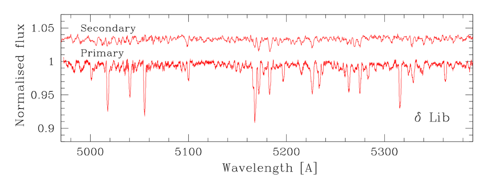
Figure 2: Disentangled spectra for the primary and secondary components in $\delta$ Lib. Metal lines in both spectra are weak but with the light ratio $l_{\rm sec}/l_{\rm prim}=0.053$ in the $V$ passband this is intrinsic for the primary’s spectrum. The weakness of the secondary’s disentangled spectrum is due to its small fractional light contribution, $l_{\rm sec}$, to the total light of the binary system.

The relative radius of star A (the radius of the star in units of the binary separation) is a large fraction of its Roche lobe, and an accretion disc cannot be formed around this component according to the Lubow & Shu (1967) criterion. No emission in H$\alpha$ was detected in the spectroscopic survey of Richards & Albright (1999). An extensive Doppler tomographic reconstruction of $\delta$ Lib (Richards et al., 2014) has revealed several components indicating activity and interaction: (i) some weak emission which is characteristic of most Algol-type systems, and is associated with the activity of a cool mass-losing component, (ii) indications of a gas stream along the predicted gravitational trajectory between the two components, and (iii) a bulge of extended absorption/emission around the mass-gaining component produced by the impact of the high-velocity stream on to the relatively slowly rotating photosphere. Compared to other Algols, $\delta$ Lib is a less ‘active’ system, as was revealed in a comprehensive tomographic study by Richards et al. (2014).

With a distance of about 95 pc, and with a cool giant secondary component, $\delta$ Lib is a bright source in the radio sky and was detected early in radio surveys (Woodsworth & Hughes, 1977; Stewart et al., 1989; Slee et al., 1987). The analysis of the continuous and long-term radio monitoring of radio flares from $\delta$ Lib confirmed its low activity, known from the optical spectral range (Richards et al., 2003). No periodicity was determined from occurrences of radio flares for $\delta$ Lib in contrast to $\beta$ Per for which some strong radio flares were detected, and the periodicity of the flares appears to be $\sim$50 d. If $\delta$ Lib were at the distance of $\beta$ Per, the radio flux of $\delta$ Lib would be much smaller than $\beta$ Per. Richards et al. (2003) explained the low level of radio flux and lower flare activity of $\delta$ Lib as being due to the higher $T_{\rm eff}$ of star B, G1 IV compared to K2 IV for $\beta$ Per. The possibility still exists that Richards et al. (2003) observed $\delta$ Lib in a quiescent period since it was found by Stewart et al. (1989) as variable radio source, whilst Singh et al. (1995) detected significant intensity variations in X-ray emission.

3 The photometric and spectroscopic observations

3.1 STEREO photometry

The NASA Solar TErrestrial RElations Observatory (stereo) was launched in October 2006 and is comprised of two nearly identical satellites (Kaiser et al., 2008). One is ahead of the Earth in its orbit (STEREO-A), the other trailing behind (STEREO-B). With their unique view of the Sun-Earth line, the STEREO mission has revealed the 3D structure of coronal mass ejections (CMEs), and traced solar activity from the Sun and its effect on the Earth. One of the principal instruments on board is the Heliospheric Imagers (HI-1) (Eyles et al., 2009). These have a large field of view, 20$\times$20^∘, and are centred 14^∘ away from the limb of the Sun. The stability of the instruments has allowed high-quality photometry of background point sources.

Over the course of an orbit almost 900 000 stars brighter than about 12 mag are imaged within 10^∘ of the ecliptic plane. Each STEREO satellite observes the stars for about 20 days with gaps of about one year. HI-1 observations have a cadence of about 40 minutes which make them very suitable for studies of eclipsing binary systems. Wraight et al. (2011) used STEREO/HI observations to detect 263 eclipsing binaries, about half of which were new detections. The LCs can be affected by solar activity. Another problem is severe blending in a crowded stellar field due to the low image resolution of about 70 arcsec.

The STEREO observations of $\delta$ Lib presented in Wraight et al. (2011) were obtained between July 2007 and Aug 2010, with a total time span of 1113 days. The quality of the photometric observations from HI-1A are of higher quality than from HI-1B, due to some systematic effects. In total 5895 measurements were obtained, of which 2802 with HI-1A imager. Due to enhanced solar coronal activity, we selected a time span the observations were clean from CMEs. The STEREO photometric measurements of $\delta$ Lib used here cover a time span of 11.80 days beginning with MJD 24554377.54433. In total 362 ($\sim$13%) measurements from the HI-1A imager smoothly covering five complete orbital cycles of the binary (Fig. 1) were adopted for the analysis in this work. These measurements needed only a small correction for detrending, and evenly cover the phased light curve. The CCDs on board the HI instruments have 2048$\times$2048 pixels, but they are binned on board to 1024$\times$1024 pixels. The pointing information in the fits headers (which were calibrated by Brown et al. 2009) was used to locate the star in an image, and then perform aperture photometry on that position. This process was repeated for all images that contain the star.

Table 1: RV measurements for our high-resolution spectra. BJD is barycentric Julian Day of midexposure. The phases are calculated with the Koch (1962) ephemeris. Subscripted 1 denotes star A, and subscripted 2 is for star B. The observatories are abbreviated as follows: AS for Asiago Astrophysical Observatory, CA for Calar Alto, TU for TUG for TÜBİTAK National Observatory, and TL for Thüringer Landessternwarte Tautenburg.

BJD	Phase	RV1	$\sigma_{1}$	RV2	$\sigma_{2}$	Obs.
54907.55260	0.243	-122.9	5.0	165.0	5.0	AS
54908.52634	0.661	22.8	5.0	-233.0	5.0	AS
54988.34355	0.957	-7.0	3.1	-	-	CA
54988.34796	0.959	0.3	1.4	-	-	CA
54988.35570	0.962	8.6	2.4	-	-	CA
54988.49871	0.023	-84.8	3.1	-	-	CA
54989.45560	0.435	-69.0	1.4	73.0	10.0	CA
54989.46330	0.438	-67.2	1.1	69.6	7.0	CA
54989.47762	0.444	-65.5	3.5	67.0	4.0	CA
54989.51552	0.460	-57.5	2.5	69.9	7.0	CA
54989.52205	0.463	-56.2	1.6	60.4	6.0	CA
54989.52855	0.466	-55.1	2.2	65.3	6.5	CA
54990.38109	0.832	27.3	1.7	-205.6	4.2	CA
54990.38659	0.835	24.9	1.4	-209.7	1.3	CA
54990.38986	0.836	25.3	1.0	-215.0	1.6	CA
54990.42792	0.852	22.2	2.0	-190.0	2.5	CA
54990.43094	0.857	20.4	2.8	-203.0	2.0	CA
54990.43398	0.855	21.1	1.9	-192.0	2.4	CA
54990.52673	0.895	7.1	3.1	-162.2	2.3	CA
54990.52991	0.896	4.4	2.1	-173.5	4.8	CA
54990.53300	0.897	4.8	3.7	-154.0	2.9	CA
54991.54431	0.332	-110.4	1.2	136.7	2.7	CA
54991.54737	0.333	-109.0	1.6	139.4	2.0	CA
54991.55274	0.336	-108.0	1.9	151.4	2.4	CA
54991.55814	0.338	-106.5	1.9	133.4	2.1	CA
55346.30550	0.763	39.0	5.0	-233.0	5.0	TU
57493.50854	0.359	-100.1	2.3	136.6	5.0	TL
57496.51161	0.649	24.0	1.1	-229.4	2.8	TL
57498.47693	0.494	-40.2	0.4	-	-	TL
57499.52097	0.942	-4.2	1.8	-74.7	5.0	TL
57499.54255	0.952	0.9	3.1	-62.2	3.3	TL
57500.46108	0.346	-103.7	2.9	135.6	6.7	TL
57502.53648	0.238	-116.7	2.8	168.7	4.3	TL
57507.52080	0.380	-93.0	0.6	125.2	5.8	TL

3.2 High-resolution échelle spectroscopy

Spectroscopic observations were secured at two observing sites. A set of 23 spectra was obtained in two observing runs (May and August 2008) at the Centro Astronónomico Hispano Alemán (CAHA) at Calar Alto, Spain. The 2.2 m telescope equipped with the foces échelle spectrograph (Pfeiffer et al., 1998) was used. The spectra cover 3700–9200 Å at a resolving power of $R\approx 40\,000$. foces used a Loral#11i CCD detector. To decrease the readout time, the spectra were binned 2$\times$2. The wavelength calibration was performed using a thorium-argon lamp, and flat-fields were obtained using a tungsten lamp. The observing conditions were generally good in both observing runs.

The spectra were bias subtracted, flat-fielded and extracted with iraf échelle package routines. Normalisation and merging of the échelle orders was performed with great care, using programs described in Kolbas et al. (2015), to ensure that these steps did not cause systematic errors in the reduced spectra.

A set of eight spectra was secured with the Coudé échelle spectrograph attached to the 2 m Alfred Jensch Telescope at the Thüringer Landessternwarte Tautenburg. They cover 4540–7540 Å at $R\approx 30\,000$. The spectrum reduction was performed using standard ESO-MIDAS packages. It included filtering of cosmic ray events, bias and straylight subtraction, optimum order extraction, flat fielding using a halogen lamp, normalisation to the local continuum, wavelength calibration using a thorium-argon lamp, and merging of the échelle orders. The spectra were corrected for small instrumental shifts using a large number of telluric O₂ lines.

4 Determination of the orbital elements

The faintness of star B relative to star A makes RV measurements difficult. Tomkin (1978) presented the first detection of star B’s spectrum in $\delta$ Lib, and the only other attempt to isolate the secondary component was presented by Bakış et al. (2006). Tomkin (1978) measured the RVs of both components from the Ca ii triplet at 8498–8662 Å. He detected star B’s spectrum in 18 of 21 available spectra obtained with the Reticon spectrograph at the 2.7 m telescope McDonald Observatory in 1977. Spectral disentangling (Simon & Sturm, 1994; Hadrava, 1995), herewith spd, was applied by Bakış et al. (2006) to derive the orbit for both components of $\delta$ Lib.

Bakış et al. (2006) used new sets of eight and nine spectra obtained on 2 m telescopes and covering a small spectral interval (6300–6750 Å) centred on H$\alpha$.

Our new observations, comprising 31 échelle spectra, were first disentangled in Fourier space (Hadrava, 1995) using the FDBinary code (Ilijić et al., 2004). Spectral disentangling clearly resolved the spectra of both components in spite the secondary component contributes much less than the primary component in the optical part of the spectrum (Fig. 2). This preliminary analysis returned the RV semiamplitudes $K_{\rm A}=78.9\pm 1.2$ km s^-1 and $K_{\rm B}=201\pm 1.8$ km s^-1, giving a mass ratio of $q=0.391\pm 0.007$.

The iSpec software (Blanco-Cuaresma et al., 2014) was used to measure RV shifts of lines with the cross-correlation method. iSpec is able to measure cross-correlation functions with a built-in spectra synthesizer for very broad spectral ranges. We used the atmospheric parameters of each component from Section 5, to measure each component separately because of a large difference between the $T_{\rm eff}$s of the components.

We also used several archival spectra of $\delta$ Lib from the Asiago and TUG observatories (İbanoǧlu et al., 2012).

For the cool secondary component, only a red part of the spectra was used since its fractional light contribution is increasing towards the red, and is about 13% in the spectral interval 6000–7000 Å.

The RV measurements are given in Table 1. Utilising the initial solution from spd, we analysed the $O-C$ residuals of the FOCES and TLS RVs separately in order to derive a possible systematic difference of the systemic velocity ($\gamma$) from two datasets. We found that the two $\gamma$s agree to within 2$\sigma$: $\gamma_{\rm CAHA}=-40.52\pm 0.37$ km s^-1 and $\gamma_{\rm TLS}=-39.65\pm 0.40$ km s^-1. An offset of $0.87\pm 0.54$ km s^-1 in the RVs between both data sets could be due to the zero-point difference between the two spectrographs, or to the influence of a third body in the system.

The presence of the third body was claimed by Worek (2001) from his comprehensive study of all available (historic) century-long RVs measurements for the primary component of $\delta$ Lib, including new observations. He derived a possible orbit of the tertiary component with the period $P=2.762$ yr, and the semi-amplitude of the changes in $\gamma$ velocities of  5 km s^-1. Our new determinations of the $\gamma$ velocity for the CAHA and TLS data sets are shown in Fig. 3. Also, in Fig. 3, we show the results for the $\gamma$ velocity determined in Bakış et al. (2006) Fig. 3 shows that the modern values of the $\gamma$ velocity contradict Worek’s solution based on historic photographic spectral plates with mostly low resolution. Our measurements corroborate the conclusion from Bakış et al. (2006) that currently the detection of the third component in the $\delta$ Lib system is not supported by spectroscopic observations.

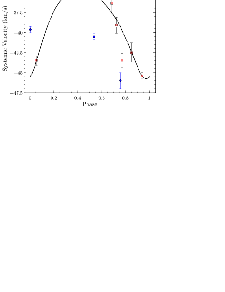
Figure 3: The variations in a systemic velocity $\gamma$. The solid line represents orbital variations due to the third body as determined by Worek (2001) from a collection of historic data and including his new observations. Data used by Worek (2001) are represented with red squares. Modern determinations of $\gamma$ from Bakış et al. (2006) and the current work are shown as blue circles, and do not corroborate the suggestion that an outer orbit with the period $P\approx 2.7$ yr exists.

In Algol-type binary systems, the cool component is filling its critical equipotential surface, i.e. in terms of the Roche equipotential surface, the system is in a semi-detached configuration. However, a tidal distortion of the Roche-lobe filling component causes non-Keplerian effects on the RV curve. The proximity distorts the component(s) from a spherically symmetric shape, and the optical centres of the stars depart from the mass centres. The elaborate analytical derivation of these tidal and rotational distortions were performed by Kopal (1980a, b). Wilson (1979) implemented a computer algorithm to calculate these effects in the widely-used wd code (Wilson & Devinney, 1971) based on the theoretical development of Wilson & Sofia (1976).

Moreover, a recent analysis of Sybilski et al. (2013) based on 12 000 simulations of binary populations shows the importance of tidal effects on the orbital parameters. They introduce the parameter $s=\frac{R_{1}+R_{2}}{a(1-e)}$ as an indicator of tidal effects and departures from Keplerian orbits. They conclude that for $s\geq 0.5$, the tidal distortion introduces a deviation up to 10 km/s on the RVs semi-amplitudes and up to 0.01 pseudo-eccentricity.

To account for the non-Keplerian effects, we use the wd code through the phoebe (Prša & Zwitter, 2005) implementation to model the RV measurements. We implemented the Markov chain Monte Carlo (herein mcmc, see Sharma (2017), and refences therein) to derive the orbital elements and their uncertainties.

As expected, the proximity effects on the RV semi-amplitude of star B are prominent, while they are negligible for the tidally undistorted star A. The difference in the RV semi-amplitude of star B between the pure Keplerian and non-Keplerian (tidally distorted) solutions amounts to about 7 km s^-1. When translated into the mass of star A, the difference is about 0.35$\,{\rm M}_{\odot}$ (c.f. Table 2).

An examination of the residuals for the Roche-lobe filling star B indicates that both models (pure Keplerian, and tidally distorted non-Keplerian) do not fully explain the RV distortions during both ingress and egress of occultations. It looks like the optical centre of star B is shifted toward the Lagrangian L2 point. Such distortion was also noticed in Bakış et al. (2006). In fact, Budding et al. (2005) have explained the distortions in the line profiles of close binary systems with the presence of circumstellar matter, which is not unexpected in Algol-type systems. As already mentioned in Sect. 2 tomographic reconstruction for $\delta$ Lib by Richards et al. (2014) revealed several structures in this particular location between the components. In the last attempt to account for distortions in star B’s RV curve we modelled the system with an artificial spot on the star, mimicking obscuring material around the L1 point in between the stars. The final fit is shown in Fig. 4 with no systematic deviations present in the residuals of either component. An obscuration (spot) has a strong impact on the RV semi-amplitude of star B, which is now $K_{\rm B}=192.0\pm 2.9$ km s^-1 (c.f. Table 2), or about 20 km s^-1 and 30 km s^-1 less than in the Keplerian and tidally deformed non-Keplerian solutions, respectively. It is well documented in the literature that spot solutions in the light curves always bear some degree of degeneracy due to an extended parameter space (cf. Morales et al. (2010)). In our mcmc calculation of spot solution, we have found a strong correlation between spot radius and the RVs semiamplitude $K_{\rm B}$ as is obvious from Fig. 5. This corelation is also projected itself to the error estimations. The uncertainity on $K_{\rm B}$ from spot solution is nearly four times bigger than those from Keplerian and tidal one (Table 2). Translated to masses, this is a drop of about 0.9$\,{\rm M}_{\odot}$ for star A compared to the pure Keplerian solution, or about 1.3$\,{\rm M}_{\odot}$ compared to the tidally deformed non-Keplerian solution. Since, star A’s RV semi-amplitude is barely affected, changes in the mass for star B are small, about 0.22 and about 0.3 $\,{\rm M}_{\odot}$ for both solutions, respectively. The geometry of the system and position of the obscured material (‘spot’) on mass-loosing component are shown in Fig. 6.

A similar effect has been detected for RZ Cas, another short-period Algol system, by Tkachenko et al. (2009). They discussed extensively the possible effects that might change the distribution of flux over the stellar disc and thus affect the RV curve. The solution could be improved taking into account the influence of a disc of variable density and a dark spot on the cool component.

Table 2: The orbital solutions for $\delta$ Lib: (a) solution for a pure Keplerian orbit, (b) tidal distortion of the Roche-lobe filling star B taking into account in the RV variations, and (c) the influence of dark obscuring material around the Lagrangian L1 point on the RV variations of star B also taking into account (a) and (b). In the calculations this obscuring cloud is represented as a dark ‘spot’ located on star B, in the direction facing star A (c.f. Fig. 6).

Param./Orb.	Keplerian	Tidal	Dark ‘spot’
KA [ km s-1]	$79.8\pm 0.5$	$79.4\pm 0.4$	$79.9\pm 0.5$
KB [ km s-1]	$211.9\pm 0.8$	$219.2\pm 0.7$	$192.0\pm 2.9$
$\gamma$ [ km s-1]	$-40.7\pm 0.1$	$-39.8\pm 0.1$	$-41.1\pm 0.1$
$q$	$0.377{\pm}0.003$	$0.362{\pm}0.002$	$0.416{\pm}0.007$
Spot (donor)
Colat. [rad]			$0.906{\pm}0.006$
Long. [rad]			$6.06\pm 0.04$
Rad. [rad]			$1.23\pm 0.08$
$T_{\rm spot}/T_{\rm B}$			$0.34\pm 0.09$
$M_{\rm A}\sin i$ [$\,{\rm M}_{\odot}$]	$4.35\pm 0.04$	$4.71\pm 0.04$	$3.42\pm 0.12$
$M_{\rm B}\sin i$ [$\,{\rm M}_{\odot}$]	$1.64\pm 0.02$	$1.71\pm 0.02$	$1.42\pm 0.03$
$a\sin i$ [$\,{\rm R}_{\odot}$]	$13.41\pm 0.04$	$13.73\pm 0.04$	$12.50\pm 0.13$

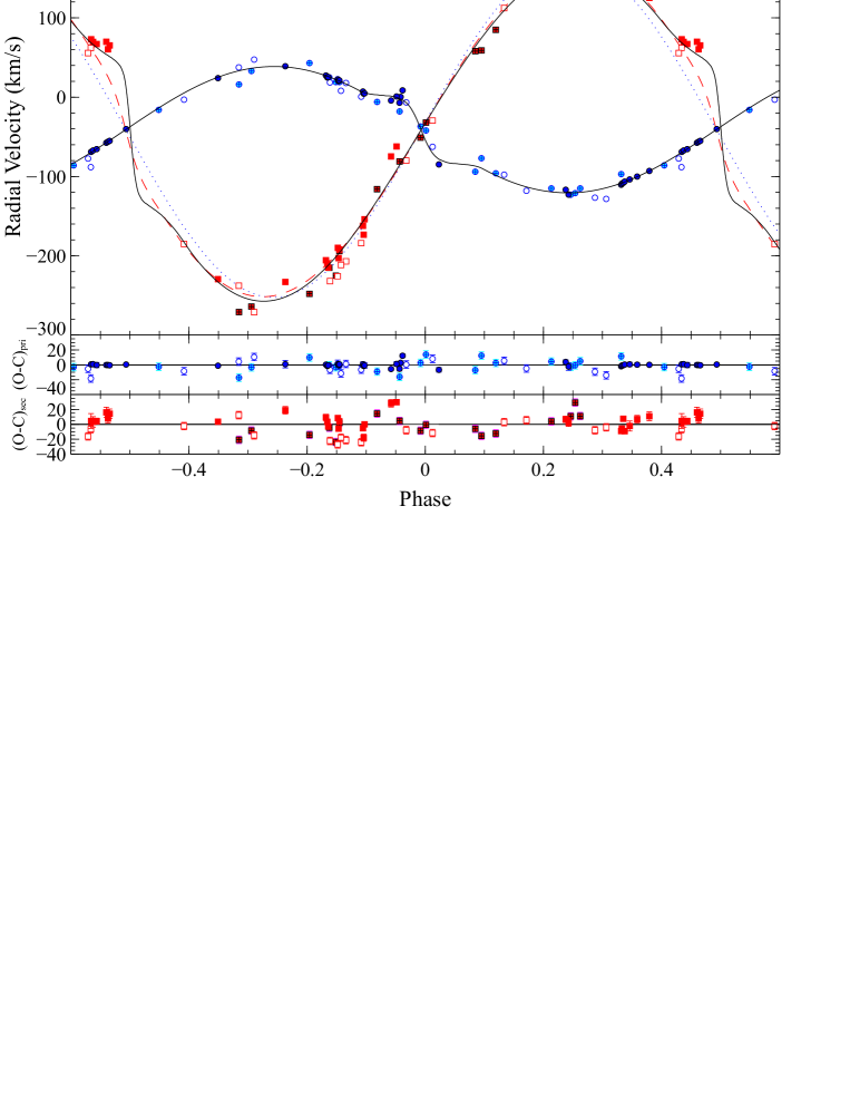
Figure 4: The best fit (solid curve) to measured RVs of star A (blue circles), and star B (red squares), with crossed symbols for Tomkin (1978), open symbols for Bakış et al. (2006), and solid symbols for our RVs measurements. In the solution non-Keplerian effects are taken into account: the RM effect during eclipses, tidal distortion of star B, and dark obscuring material between the components, around the Lagrangian L1 point. The solutions for a pure Keplerian orbit (dotted curve), and with tidal effects on both stars (dashed curve) are also shown for comparison.

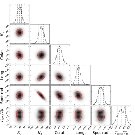
Figure 5: The determination of the orbital and spot parameters and accompaning uncertainties from measured RVs using phoebe code. Distribution and correlation of these parameters from the $10^{6}$ mcmc runs are shown. Degeneracy in determination of the temperature ratio $T_{\rm spot}/T_{\rm B}$ is clearly seen. Also, a strong correlation between spot radius and the RV semiamplitude of star B (mass-loosing component) is present. In each section, the map of distribution densities between parameters are plotted with associated 1 $\sigma$ and 2 $\sigma$ confidence levels (solid countours). The histogram distributions (solid lines) are plotted across the associated variable. Mean and 1 $\sigma$ of each variable are indicated with dashed lines.

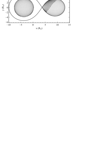
Figure 6: Roche geometry for the $\delta$ Lib system. The secondary, less massive and cooler component is filling its Roche lobe, whilst the primary component is detached from its Roche lobe. The position of the obscuring material in the vicinity of the L1 point, modelled as a dark spot on the secondary component, is indicated.

5 Atmospheric parameters for the components

As described in the preceding section, due to the non-Keplerian effects on the RV variations of the components in the $\delta$ Lib system, plus the prominent Rossiter-McLaughlin (RM) effect, i.e. line profiles distortions in the course of the eclipses (Rossiter, 1924; McLaughlin, 1924), spectral disentangling in its complete form, i.e. determination of the orbital elements, and reconstruction of the individual spectra of the components, cannot be applied. Therefore, spectral disentangling was performed in a pure separation mode (c.f. Pavlovski & Hensberge, 2010) using the RVs measured by cross-correlation (Table 1), and cres code (Ilijić, 2004) based on the spd method of Simon & Sturm (1994). Although the spectra are separated, the continuum is still composed of the light from both stars. To determine the atmospheric parameters the disentangled spectra should be renormalised to their own continuum. One possibility is to use the light ratio between the components from the LC analysis (c.f. , Hensberge et al.2000). The other is a direct optimal fitting of disentangled spectra in which the light ratio is to be determined too. Information on the light ratio is preserved in disentangled spectra, as well as projected rotational velocity (Tamajo et al., 2011).

In the present analysis, we used both options and obtained very consistent results. The starfit code (Kolbas et al., 2014) is used for the optimal fitting of the disentangled spectrum of star A. Star B contributes little to the total light of binary system, about 5–9 per cent in the optical part, and with a rather limited number of spectra available for spd its disentangled spectrum suffers from a low S/N.

Three hydrogen lines exist in the spectral range of the disentangled spectrum of star A: H$\beta$, H$\gamma$, and H$\delta$ (Fig. 7). The starfit code searches a large 2D grid ($T_{\rm eff}$ v. $\log g$) of pre-calculated theoretical spectra, and compares them to the disentangled spectrum. The following parameters can be obtained: $T_{\rm eff}$, surface gravity $\log g$, light dilution factor $ldf$, projected rotational velocity $v\sin i$, relative velocity shift between the disentangled spectrum and the laboratory rest-frame wavelengths of the theoretical spectra $v_{0}$, and the continuum offset correction $ccor$. For the optimisation of these parameters a genetic algorithm (Charbonneau, 1995) is adopted. The grid of theoretical spectra are calculated in LTE with the program uclsyn (Smith, 1992; Smalley et al., 2001).

In the course of the present study, a Monte Carlo Markov Chain (MCMC) algorithm for the calculations of the uncertainties in the optimal fitting of the disentangled spectra has been implemented in the starfit code. The most general MCMC algorithm is the Metropolis-Hasting (MH) algorithm (Metropolis et al., 1953; Hastings, 1970) which was used for the error analysis (c.f. Hogg & Foreman-Mackey (2018), and references therein). For the simulation, we used at least $10^{5}$ steps after the burn-in phase. To ensure good mixing in the Markov chain, we used an adaptive step in our algorithm and ensured our acceptance ratio was bigger than 0.279 as suggested by Sharma (2017).

Table 3: Atmospheric parameters for $\delta$ Lib A determined from optimal fitting of disentangled spectra centred on the Balmer lines.

Spectral line: H$\beta$	Unit	Optimisation 1	Optimisation 2	Optimisation 3
Effective temperature, $T_{\rm eff}$	K	$10562\pm 60$	$10560\pm 60$	$10519\pm 30.4$
Surface gravity, $\log g$	[cgs]	$3.835\pm 0.008$	3.84 fixed	3.84 fixed
Light dilution factor, $ldf$		$0.938\pm 0.009$	$0.937\pm 0.009$	Normalised
Projected rotational velocity, $v\sin i$	km/s	$72.52\pm 3.18$	$72\pm 3$	73 fixed
Spctral line: H$\beta$ Degenerate solution
Effective temperature, $T_{\rm eff}$	K	$9914\pm 54$	–	–
Surface gravity, $\log g$	[cgs]	$3.573\pm 0.005$	–	–
Light dilution factor, $ldf$		$0.918\pm 0.008$	–	–
Projected rotational velocity, $v\sin i$	km/s	$73.80\pm 2.77$	–	–
Spectral line: H$\gamma$
Effective temperature, $T_{\rm eff}$	K	$10756\pm 158$	$10770\pm 60$	$10550\pm 66.1$
Surface gravity, $\log g$	[cgs]	$3.82\pm 0.04$	3.84 fixed	3.84 fixed
Light dilution factor, $ldf$		$0.984\pm 0.021$	$0.984\pm 0.009$	Normalised
Projected rotational velocity, $v\sin i$	km/s	$73.4\pm 6.5$	$73\pm 6$	73 fixed
Spectral line: H$\delta$
Effective temperature, $T_{\rm eff}$	K	$10724\pm 149$	$10610\pm 150$	$10484\pm 82$
Surface gravity, $\log g$	[cgs]	$3.94\pm 0.03$	3.84 fixed	3.84 fixed
Light dilution factor, $ldf$		$0.967\pm 0.022$	$0.965\pm 0.025$	Normalised
Projected rotational velocity, $v\sin i$	km/s	$82.0\pm 12.7$	$82\pm 10$	73 fixed
Adopted weighted $T_{\rm eff}$	K			$10520\pm 110$

As mentioned above Lazaro et al. (2002) determined the $T_{\rm eff}$ and $\log g$ for star A from photometric indices. Various calibrations have restricted $T_{\rm eff}$ to between 9650 and 10 500 K, and $\log g$ to between 3.75 and 4.0. In this $T_{\rm eff}$ range the degeneracy between $T_{\rm eff}$ and $\log g$ is present for the strong and broad Balmer lines. However, in eclipsing and double-lined spectroscopic binaries the masses and radii could be determined with high accuracy, and the degeneracy between $T_{\rm eff}$ and $\log g$ in the wings of the Balmer lines can be lifted with a precisely determined $\log g$. The LC analysis also provides the light ratio between the components thus making determination of the $T_{\rm eff}$ from disentangled spectra more certain. In this work, we performed an optimal fitting of the disentangled primary’s spectrum using three methods: (1) all parameters free, (2) $\log g$ fixed, and (3) $\log g$ and light dilution factor fixed. These parameters are listed in Tables 5 and LABEL:tab:abspar. Only a few iterations were needed to converge to the final values. The results of all three fits are given in Table 3.

As expected, the solutions for option (1) are degenerate. In Table 3 both solutions are given for the H$\beta$ line. This is also illustrated in Fig. 8 in which two solutions are clearly distinguishable, one at $T_{\rm eff}=9910$ K and $\log g=3.57$, and the other at $T_{\rm eff}=10\,560$ K and $\log g=3.84$. It is interesting that in the second solution the $\log g$ matches perfectly the value determined from the primary’s dynamical mass and radius from the LC solution. Without the possibility to obtain the $\log g$ from combined RVs and LC analysis, the atmospheric parameters could be erroneous due to a strong degeneracy between the $T_{\rm eff}$ and $\log g$ in the Balmer lines for hot stars. It is also encouraging that fixing $\log g$ gives a light dilution factor in perfect concordance with the LC solution (optimisation 2 in Table 3).

Having lifted the degeneracy between $T_{\rm eff}$ and $\log g$, and with an appropriate renormalisation of the disentangled spectra using the light ratio from the photometric analysis, the uncertainties in the determination of $T_{\rm eff}$ have been reduced. This is important, first, for the quality of the LC solution, and, second, for proper calculations of the model atmospheres and the determination of photospheric abundances. Since the LC solution and the $T_{\rm eff}$ determination from the disentangled spectra are interconnected, an iterative approach is needed. Convergence was fast, and only a couple of iterations were needed for consistent solutions. The quality of the fits for the Balmer lines, H$\delta$, H$\gamma$, and H$\beta$ are shown in Fig. 7.

Projected rotational velocities, $v\sin i$, for both components were determined with starfit by fitting metal lines. The Balmer lines and severely blended metal lines were masked. Such fitting gives $v\sin i=72.5\pm 3.2$ km s^-1. Two previous results for star A’s $v\sin i$ were published: Cugier (1989) determined $v\sin i=75$ km s^-1 (with no uncertainty), whilst Parthasarathy et al. (1983) found a slightly lower value of $v\sin i=69\pm 4$ km s^-1. Our determination is within 1$\sigma$ of both values.

The large uncertainty in determination of star B’s $v\sin i$ does not allow any further discussion on its implication for constraining the mass ratio through rotational synchronisation of this Roche-lobe filling component.

In the renormalisation of the disentangled spectra for star B, the multiplicative factor is large (about 11 and 20 in $V$ and $B$ passbands, respectively) due to its small contribution to the total light of the system. Accordingly the noise is multiplied, and determination of the atmospheric parameters is less reliable than from the LC analysis (Tables 5 and LABEL:tab:abspar). Still, we are interested to see if the optimal fitting would give a sensible solution. The starfit solution with the MCMC error calculations gives the following atmospheric parameters for the faint secondary component: $T_{\rm eff}=5095\pm 280$ K, $\log g=3.48\pm 0.07$, $ldf=0.052\pm 0.009$, and $v\sin i=94\pm 12$ km s^-1. This should be compared with the values we adopted in the present work from the RVs and LC modelling: $T_{\rm eff}=5134\pm 240$ K, $\log g=3.48\pm 0.06$, $ldf=0.068\pm 0.015$ (interpolated between $B$ and $V$ passbands in Table 5).

Figure 7: The best-fitting synthetic spectra (lines) compared to the renormalised disentangled spectra (filled circles) of star A. H$\beta$ (upper), H$\gamma$ and H$\delta$(lower) profiles are shown with offsets for clarity.

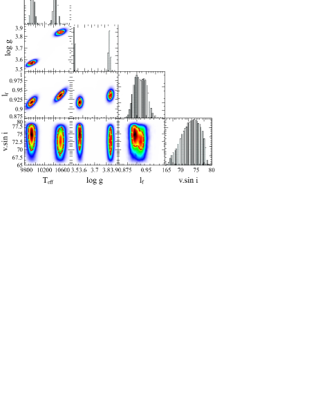
Figure 8: The determination of atmospheric parameters with MCMC through 10⁶ steps from the H$\beta$ line. Degeneracy in the solution is obvious, and external information is needed to break it. We used precise determination of $\log g$ from the combined RV and LC analysis which then yield star A’s $T_{\rm eff}$. Different options in an optimal fitting of the Balmer lines are given in Table 3.

6 Light curve analysis

The following photometric observations of $\delta$ Lib are used in the light curve analysis (see Section 2):

• Broadband photoelectric photometry of Koch (1962). These total 337 measurements in $U$, 338 in $B$, and 343 in $V$.

• Strömgren $y$ photometry from Shobbrook (2004), which has been transformed to the Johnson $V$ passband. The dataset consists of 111 measurements that are fairly well distributed in orbital phase.

• The Hipparcos data comprise 89 measurements in the original Hipparcos passband and transformed to Johnson $V$ (Harmanec, 1998).

• Infrared $JHK$ photometry of Lazaro et al. (2002). The majority of the observations are in the $JHK$ filters with a few measurements in $L$. In total, the photometry consists of 722 measurements in $J$, 783 in $H$, and 770 in $K$.

• Broadband photometry extracted from the STEREO/ Heliospheric Imagers images (Eyles et al., 2009). The data acquisition is described in Sect. 3.1.

We used the phoebe suite 0.31a (Prša & Zwitter, 2005), which is based on work by Wilson & Devinney (1971) and generalized by Wilson (1979), to find a solution to the LCs. The mass ratio $q=0.416\pm 0.007$ is determined in Sect. 4, and was fixed in the analysis of the LCs. Since the $\delta$ Lib system is in a semi-detached configuration, the radius of star B is defined by the mass ratio and the geometry of the system. Thus mode 5 (semi-detached binary with the secondary component filling its Roche lobe) was used in the calculations. The $T_{\rm eff}$ for star A is determined from the optimal fitting of its disentangled spectrum (Sect. 5), In the final runs we fixed it to $T_{\rm eff,\,A}=10\,520$ K. Gravity-darkening coefficients were set to $g_{\rm A}=1.0$ and $g_{\rm B}=0.32$ which is appropriate for radiative (von Zeipel, 1924), and convective envelopes (Lucy, 1967), respectively. In accordance with the properties of the atmospheres, we kept fixed the bolometric albedos $A_{\rm A}=1$ and $A_{\rm B}=0.5$ after Rucinski (1969). phoebe’s implementation of logarithmic limb darkening interpolation uses van Hamme (1993) tables, with the exception of the $H$ passband which was taken from Claret (2000).

The following parameters were left free for adjustment in the LC calculations: the $T_{\rm eff}$ of star B ($T_{\rm eff,B}$), the surface potential of star A $\Omega_{\rm A}$ (i.e. its relative radius $r_{\rm A}$), and the orbital inclination $i$. Table 4 provides the list of fixed parameters during this analysis. The orbital phases are calculated with the ephemeris given by Koch (1962). The best fit and the uncertainties for adjusted parameters are then calculated with phoebe with the mcmc implementation.

Table 4: The fixed system parameters of $\delta$ Lib during the lightcurve analysis.

Parameter	Unit	Value
Orbital period $P$	d	$2.32735297$
Primary eclipse time HJD	d	$2\,422\,852.3598$
Mass ratio $q$		$0.416\pm 0.007$
$T_{\rm eff}$ of star A	K	$10\,520\pm 110$
Gravity darkening (A,B)		$1.0$, $0.32$
Bolometric albedo (A,B)		$1.0$, $0.5$
Third light		$0.0$

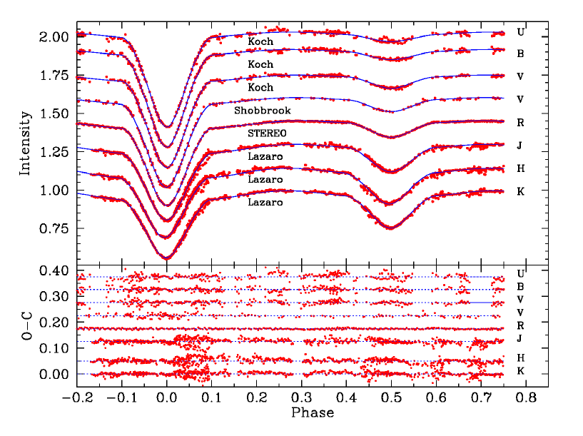
Figure 9: Observed phased LCs of $\delta$ Lib (solid dots) with the best-fitting phoebe model LCs (continuous line) with associated passband and observer labels (top panel). In the lower panel the residuals have been plotted to show the quality of the fit. Both lightcurves and residuals are shifted for the ease of viewing. The phases are calculated using the Koch (1962) ephemeris. A small adjustment of the phases was needed, and was included in the LC analysis.

For this purpose we wrote a home-made script for phoebe to produce the mcmc simulations. This script uses the Metropolis-Hastings algorithm to accept or reject the proposed value of the orbital parameters to find the most probable fitting model and associated errors. To calculate the acceptance ratios, we used the observational error (scatter of residuals) of the best-fitting parameter from the differential corrections algorithm in the WD code.

With starting random initial parameters and $10^{5}$ simulations for each LC after the burn-in phase, the uncertainties $\sigma$ for each free parameter are calculated from the normal distribution of accepted results.

Altogether, eight LCs are solved using the described procedure ($UBV$ from Koch (1962), $V$ from Shobbrook (2004) and Hipparcos, stereo LC in the $R$ band from the present study (see also Wraight et al. (2011), and the $JHK$ data from Lazaro et al. (2002).) The LCs, best fitting models and residuals are shown in Fig. 9. The optimal parameters from phoebe (as shown in Fig. 9) and the uncertainties from the mcmc calculations are given in Table 5.

Table 5: Results from the solution of the wd modelling, mcmc analysis with associated $\sigma$ values for the free parameters, namely inclination, the $T_{\rm eff}$ of star B and the radius of star A. The light fraction and its errorbar for star A ($l_{f}=L_{\rm A}/(L_{\rm A}+L_{\rm B})$) and the scatter of the residuals of the fits are also listed.

Band	$r_{\rm A}$	$i$ [deg]	$T_{\rm B}$ [K]	$l_{\rm A}$	$\sigma$ [flux]
$U$	0.300	80.6	5468	0.9610	0.0300
	$\pm$0.005	$\pm$0.25	$\pm$182	$\pm$0.0004
$B$	0.300	80.5	5416	0.9520	0.0152
	$\pm$0.003	$\pm$0.1	$\pm$86	$\pm$0.0005
$V$	0.293	80.1	5261	0.9112	0.0150
	$\pm$0.003	$\pm$0.1	$\pm$60	$\pm$0.0010
$H_{p}$	0.301	79.8	5309	0.9120	0.0130
	$\pm$0.003	$\pm$0.13	$\pm$94	$\pm$0.0011
$R$	0.296	79.22	5126	0.8760	0.0048
	$\pm$0.001	$\pm$0.05	$\pm$17	$\pm$0.0006
$J$	0.296	79.17	5092	0.7574	0.0196
	$\pm$0.004	$\pm$0.11	$\pm$31	$\pm$0.0052
$H$	0.293	79.33	4994	0.6660	0.0220
	$\pm$0.005	$\pm$0.12	$\pm$44	$\pm$0.0114
$K$	0.299	79.15	5204	0.6544	0.0176
	$\pm$0.004	$\pm$0.11	$\pm$40	$\pm$0.0084
Mean	0.297	79.45	5134	-	-
$\sigma$	$\pm$0.010	$\pm$0.37	$\pm$ 240	-	-

Table 6: The absolute dimensions and related quantities determined for $\delta$ Lib. $V_{\rm synch}$ is the calculated synchronous rotational velocity.

Parameter	Unit	Star A	Star B
Mass	$\,{\rm M}_{\odot}$	$3.60\pm 0.13$	$1.50\pm 0.04$
Radius	$\,{\rm R}_{\odot}$	$3.78\pm 0.13$	$3.79\pm 0.04$
$\log g$	cm s-2	$3.84\pm 0.03$	$3.46\pm 0.01$
$T_{\rm eff}$	K	$10\,520\pm 110$	$5\,150\pm 175$
$\log L$	L⊙	$2.19\pm 0.03$	$0.96\pm 0.06$
$V_{\rm eq}$ $\sin i$	km s-1	$72.5\pm 3.2$	$94\pm 12$
$V_{\rm synch}$	km s-1	$82.1\pm 2.9$	$82.3\pm 1.0$

7 Abundance Analysis

$\delta$ Lib A contributes the highest proportion of light to the total light of the binary system. Renormalisation of its disentangled spectrum degrades the S/N only slightly, which is not the case for $\delta$ Lib B. Thus, determination of the photospheric abundances was possible only for star A. The atmospheric parameters ($T_{\rm eff}$ and $\log g$), needed for the set-up of the model atmosphere are determined from an optimal fitting of star A’s renormalised disentangled spectrum with fixed $\log g$, and calculated from its dynamical mass and radius determined from the LC analysis (Sections 4 and 6).

Due to the star A’s relatively high $v\sin i$ of $72.5\pm 3.2$ km s^-1, the spectral lines are broadened and blended. Only a few spectral lines, mostly of Fe ii, are free of contamination, but their numbers are too low to determine the microturbulence velocity $\xi$ from the EWs. Instead, the elemental abundances were determined by an optimal fitting of selected line blends, for a fixed $\xi=1.5$ km s^-1. We adopted this value from the calibration work of Gebran et al. (2014). We selected line blends which are not too crowded, and which contain the CNO species of particular interest.

We used the uclsyn code (Smalley et al., 2001) which allows a simultaneous fit for the five different atoms or ions. For such complex blends we iterated several times, usually starting iterations with different initial compositions. The line list and atomic data are compiled from the VALD database (Piskunov et al., 1995; Kupka et al., 1999).

In Table 7, derived elemental abundances for star A are given. The uncertainties are calculated from a scatter (standard deviation) in the measurements for different lines and from differences in the abundances due to the uncertainties in the $T_{\rm eff}$ ($\pm 110$ K) and $\log g$ ($\pm 0.023$). Also, we have taken into account the uncertainty in $\xi$ which we estimated as $\pm 0.10$ km s^-1.

Since the uclsyn code gives the rms values for each line, we calculated a grid of models within an error of the atmospheric parameters given above. We then used these solutions to find the scatter around our most probable solution. The uncertainties in star A’s atmospheric parameters have a small contribution to the uncertainties in abundances which come mostly from the scatter from the spectral lines used in the determination. The abundances relative to solar composition given by Asplund et al. (2009) are also given for comparison.

It turns out that the iron abundance [Fe/H] $=0.16\pm 0.10$ is larger than the solar abundance. An average photospheric abundance for metals (Mg, Si, Ti, Cr, and Fe) is [M/H] $=0.16\pm 0.13$, and supports the case for a higher metallicity determined for iron alone. Unfortunately in previous research the iron abundance was not determined and comparison is not possible. Cugier (1989) determined the carbon abundance from C ii resonant lines in the ultraviolet spectral region at 1335–1337 Å from the IUE satellite spectra. He found values of $\log\epsilon{\rm(C)}=8.42\pm 0.15$ in LTE, and $\log\epsilon{\rm(C)}=8.36\pm 0.20$ and $\log\epsilon{\rm(C)}=8.45\pm 0.20$ in NLTE, for the complete and partial redistribution, respectively. All Cugier’s determinations are for these atmospheric parameters: $T_{\rm eff}=9900\pm 200$ K, $\log g=4.00\pm 0.10$, and $\xi=2$ km s^-1, and are determined from the ultraviolet flux distribution. Our determination is in almost perfect agreement with the carbon abundance determined by Cugier (1989), and also supports his conclusion of a solar standard value which is in modern evaluation $\log\epsilon{\rm(C)_{\odot}}=8.43\pm 0.05$ (Asplund et al., 2009). The carbon abundance for $\delta$ Lib A was also estimated by Parthasarathy et al. (1983). Their work was based on the analysis of the C ii 4247 Å line. They found it rather weak in the spectrum, and gave only an upper limit of $\log\epsilon{\rm(C)}\leq 8.52\pm 0.15$. This upper limit is within the uncertainty of 1$\sigma$ for both Cugier (1989) and our measurements.

The enrichments of nitrogen and oxygen are obvious from our measurements, with $\log\epsilon{\rm(N)}=8.23\pm 0.06$, and $\log\epsilon{\rm(O)}=9.03\pm 0.06$. The carbon-to-nitrogen abundance ratio is particularly important for our evolutionary modelling, which are given from our abundance determination (Table 7) as $\log$ C/N $=0.19\pm 0.09$, i.e. C/N $=1.55\pm 0.40$.

Table 7: Photospheric abundances derived for $\delta$ Lib A. Abundances are expressed relative to the abundance of hydrogen, $\log\epsilon(H)=12.0$. The third column gives the number of lines used. The fifth column lists the solar abundances from Asplund et al. (2009) which are used as reference values.

El	A	$N_{\rm li}$	$\log\epsilon({\rm X})$	Solar	[X/H]
C	6	6	8.42$\pm$ 0.11	8.43 $\pm$ 0.05	-0.01 $\pm$0.09
N	7	5	8.23 $\pm$ 0.06	7.83 $\pm$ 0.05	0.40 $\pm$0.06
O	8	15	9.03 $\pm$ 0.06	8.69 $\pm$ 0.05	0.34 $\pm$0.06
Mg	12	11	7.76 $\pm$ 0.17	7.60 $\pm$ 0.04	0.16 $\pm$0.12
Si	14	7	7.67 $\pm$ 0.19	7.51 $\pm$ 0.03	0.16 $\pm$0.14
Ti	22	23	5.21 $\pm$ 0.22	4.95 $\pm$ 0.05	0.26 $\pm$0.16
Cr	24	15	5.70 $\pm$ 0.13	5.64 $\pm$ 0.04	0.06 $\pm$0.10
Fe	26	146	7.65 $\pm$ 0.13	7.50 $\pm$ 0.04	0.15 $\pm$0.10

8 Evolutionary Analyses

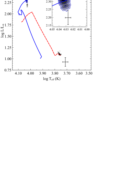
Figure 10: The best fitting evolutionary tracks for the $\delta$ Lib mass-gainer (solid) and mass-loser (dashed) associated with empirical values from Table LABEL:tab:abspar. Density contours of all acceptable solutions are overplotted. The region around the mass-gainer is shown zoomed-in for clarity.

Evolutionary calculations that includes binary interactions (such as mass transfer, tidal sysnchronisations) have been done since mid-sixties (e.g. Kippenhahn & Weigert (1967), Plavec (1970), Plavec et al. (1973), Paczyński (1971)). Currently, there are numerious groups conducted with different stellar evolution codes to model stellar response to the abrupt mass change triggered by Roche Lobe overflow (van Rensbergen et al. (2006), Stancliffe & Eldridge (2009), Siess et al. (2013), Paxton et al. (2015)) which most of them give similar results for accretion on non-degenerate stars. In general, the main uncertinities faced in modelling binary evolution is to reckoning the efficiency of mass transfer (i.e the mass loss from system) and the angular momentum loss. The problem is relatively easy for Algol-type systems since they are supposedly passed only one RLOF induced mass transfer. However, even with the mass-angular momentum conservation assumtion, one needs to take the initial mass ratio of system as free parameter. The best way to overcome such problem is to build sets of models with various systemic initial mass ratios and compare the evolution tracks with observations. The number of proposed models increased with power of free parameters when we also innclude the mass and angular momentum loss.

In the evolutionary analyses of binary stars, two different methodologies are often applied. The first one uses a large grid of binary evolution models which are calculated for a range of initial components’ masses and periods to find the initial conditions which produce the observed properties (masses, $T_{\rm eff}$  radii, orbital period, etc.) of the current system by comparing them with calculated models, and finds the best match. This method is generally well suited to the analysis of a large sample of systems, and has been successfully applied by Nelson & Eggleton (2001) and de Mink et al. (2007). The second approach calculates a series of models for a given system by guessing all possible initial configurations with angular momentum and mass loss assumptions and building binary evolution grids to find the best match. Nowadays this CPU-intensive method is possible thanks to modern computing power (Kolbas et al., 2014).

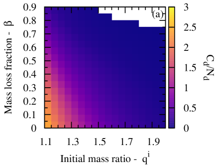
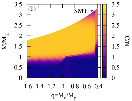
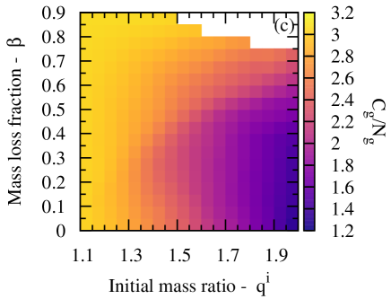
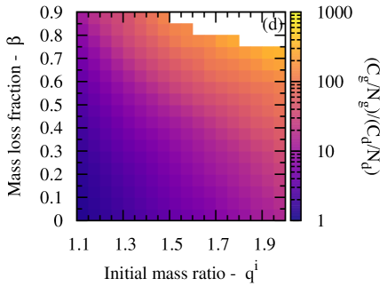
Figure 11: The surface C/N yield of the mass-loser through grid is shown in panel (a) with associated colour scale. The interior C/N profile of the mass-gainer during the mass transfer, i.e. from higher mass ratio to lower one, is shown in panel (b). The end of rapid mass transfer (SMT) is annotated. The surface C/N yield of the mass-gainer through the grid is also shown in panel (c). While the individual outcome of the components’ C/N ratio can be similar for a given $q^{i}$ and $\beta$, the ratio of the C/N ratios for the mass loser and gainer could be a good diagnostic to resolve the degeneracy in the system, as shown in panel (d).

The calculations of the evolutionary models were undertaken following the method and conventions presented in Kolbas et al. (2014). The input ingredients of a model for a given metallicity are: the final masses of the components ($M_{d}^{f}$, $M_{g}^{f}$), thus the final mass ratio ($q^{f}=$ $M_{d}^{f}/M_{g}^{f}$), and the final orbital period ($P^{f}$). Then, the calculated quantities are the initial mass of the donor ($M_{d}^{i}$), the initial mass of the gainer ($M_{g}^{i}$), and the initial orbital period ($P^{i}$) of the system for a given initial mass ratio ($q^{i}=$ $M_{d}^{i}/M_{g}^{i}$), and the mass transfer efficiency parameter ($\beta$). Using the assumption that mass loss (i.e. $(1-\beta)\,dM_{d}$) carries the angular momentum away from the donor (Hurley et al., 2002; Kolbas et al., 2014), a simple relation between the period, the total mass, and the components’ masses is derived. Namely $P\,M_{t}^{2}\,M_{g}^{3}\,M_{d}^{3(1-\beta)}={\rm const}$ during the orbital evolution.

Then the initial period of system can be derived from the equation

$$P^{i}=P^{f}\left(\frac{M_{t}^{f}}{M_{t}^{i}}\right)^{2}\left(\frac{M_{g}^{f}}{M_{g}^{i}}\right)^{3}\left(\frac{M_{d}^{f}}{M_{d}^{i}}\right)^{3(1-\beta)}$$ (1)

where

$$M_{t}^{i}=M_{t}^{f}\frac{(1+q^{i})}{(1+q^{f})}\frac{[1+q^{f}(1-\beta)]}{[1+q^{i}(1-\beta)]}.$$ (2)

is the systemic mass equation as a function of initial and final mass ratio (Giuricin & Mardirossian, 1981).

Equations (1) and (2) also give the well-known equivalent relations for the assumptions of mass (i.e. $\beta=0$) and angular momentum conservations. As one can see, since the final parameters of the system (i.e., $M_{d}^{f}$,$M_{g}^{f}$, $M_{t}^{f}$, $q^{f}$, $P^{f}$) are known, the only unknowns are $q^{i}$ and $\beta$ which are taken to be free parameters.

Thus, using Eq. (1) and Eq. (2), one can calculate the possible initial parameters of a system (i.e., $M_{d}^{i}$, $M_{g}^{i}$, $M_{t}^{i}$, $P^{i}$) for various $q^{i}$ and $\beta$ values. These parameters can be used to build a grid of evolutionary tracks which allows us to compare, the current absolute parameters of the system ($M_{\rm A}$, $M_{\rm B}$, $T_{\rm eff,A}$, $T_{\rm eff,B}$, $R_{\rm A}$, $R_{\rm B}$) to find the best fitting models with accompanying $q^{i}$ and $\beta$.

Although the value of the efficiency parameters could be between $0\leq\beta\leq 1$ (i.e. from conservative to totally non-conservative mass transfer), we found for $\delta$ Lib that some of the initial periods with $\beta\gtrsim 0.8$ for a given $q^{i}$ are lower than the limiting period (Nelson & Eggleton, 2001) for a given binary system, namely

$$P_{\rm lim}\approx\frac{0.19M_{g}^{i}+0.47{M_{g}^{i}}^{2.33}}{1+1.18{M_{g}^{i}}^{2}}.$$ (3)

Thus we excluded all the initial parameters with $P^{i}\leq P_{\rm lim}$ from our analysis.

As also implied from Eq. (1), mass transfer leads to fast increase of the orbital period after mass ratio reversal. Thus $\delta$ Lib must have had a short initial orbital period to explain its current period. This situation constrains the number of initial parameters.

For the initial mass ratio, we used the mean mass ratio of detached binaries from İbanoǧlu et al. (2012) as a lower limit ($q^{i}\approx 1.1$). As a result of such consideration, we calculated the initial parameters of the system as $\beta=[0.0-0.9]$ with an increment size of $\delta\beta=0.05$ and $q^{i}=[1.1-2.0]$ with an increment size of $\delta q^{i}=0.05$ which constructs a 18$\times$18 matrix grid size. This is considerably higher resolution than those of Kolbas et al. (2014) which used a 4x5 grid size.

The Cambridge version of the stars evolution code was used for model calculations. stars was originally developed by Eggleton (1971, 1972) to calculate the evolutionary tracks for the initial parameters, $q^{i}$ and $\beta$. The code was substantially upgraded for both new EOS tables and the capability of simultaneous calculation for both components of a binary system (Pols et al., 1995; Stancliffe & Eldridge, 2009). In our calculations, solar composition for both components is assumed, and the overshooting parameter is kept fixed at $\delta_{os}\sim 0.12$.

We have run the code until the second mass transfer has occurred which is assumed to be the end of algolism for binary systems. Considering that every initial configuration set produces approximately 5000 interior models for each component, we have more than 3 000 000 models of stellar interiors to compare to find the best fitting one.

For each initial set of masses and periods, we calculated the $\chi^{2}$ of the corresponding evolutionary tracks. Then we compared the minimum $\chi^{2}$ of every set of initial parameters with each other to find the best fitting model pair which matches both components with same age. We also calculated the likelihood of each minimum $\chi^{2}$ based on the derived errors of both components of the $\delta$ Lib system which are given in Table LABEL:tab:abspar.

The components’ physical parameters were derived from Fig. 10 showing the HR diagram of the best fitting model tracks of both components together with the confidence countours from likelihood analysis. We plot the HR diagram of the best-fitting set of model tracks, confidence contours from the likelihood analysis and the derived physical parameters of the components in Fig. 10.

As a result of this, we determine the parameters of the best fitting model as $q^{i}=1.60$ and $\beta=0.0$. Using likelihood calculations, we determined the most probable initial parameters and associated errors as $\langle q^{i}\rangle=1.626\pm 0.125$ and $\langle\beta\rangle=0.142\pm 0.11$. Thus we determine the initial mass of the gainer and the period of the system as $M_{d}^{i}=3.028\pm 0.161$ $\,{\rm M}_{\odot}$ and $P^{i}=1.3531\pm 0.099$ d.

This result is based on absolute parameters. From the abundance analyses we also know that C/N$=1.55\pm 0.4$, which can be used for constraining the previous determination. So taking into account the thermohaline constraint, we limited the posible sets of initial conditions to those which satisfy the C/N ratio within an uncertainty range and determine the expected initial parameters $\langle q^{i}\rangle=1.765\pm 0.071$ and $\langle\beta\rangle=0.13\pm 0.11$. This yields the initial mass of the gainer and the period of the system as $M_{d}^{i}=3.116\pm 0.161$ $\,{\rm M}_{\odot}$ and $P^{i}=1.435\pm 0.108$ d. From both of these results we conclude that $\delta$ Lib has experienced a conservative to very mildly non-conservative evolution.

It is our principal interest to compare the chemical evolution outcome of the models with the results of the abundance determination for species that are most sensitive to CNO processing and mixing in stellar interiors prior to mass transfer. As was explained in the Introduction, C and N suffer the largest changes, and in some sense N becomes overabundant at the expense of C. For this purpose, we extracted the C/N ratios for each component from the minimum-$\chi^{2}$ models of every set of $q^{i}$ and $\beta$. In Fig. 11a we show the outcomes for the mass donor’s surface C/N ratio after mass transfer stripped the outer layers. The surface C/N ratio is lower than the solar value of (C/N)${}_{\odot}\approx$ 2.8 and decreases with increasing $q^{i}$ and $\beta$ down to C/N $\sim$ 0.01.

As we mentioned, the mass reversal leads to a period increase during the orbital evolution and thus ends the rapid phase of mass transfer. Since in non-conservative cases, a part of the transferred mass is not accreted, mass reversal occurs later than for conservative cases. This is a natural result of non-conservative orbital dynamics which leads to a postponed mass reversal and thus deeper layers are exposed.

As the mass ratio decreases in the course of the mass transfer, the deeper layers which contain nuclear processed material from the CNO cycle are exposed shortly after the mass ratio reversal has occurred. Based on the best fit parameters, it is expected that the surface C/N${}_{d}=0.35\pm 0.2$. Unfortunately, due to the small contribution of the donor to the total light of the $\delta$ Lib system, about 6 per cent (Table 5), the S/N of the donor’s disentangled spectrum is not sufficient for a detailed abundance analysis with the required precision.

Once mass transfer begins, the $1-\beta$ fraction of the lost matter from the donor will be accreted by the gainer. As we have already shown, the accreted donor’s material will have a different C/N ratio than that of the surface of the gainer which satisfies the starting condition of thermohaline mixing as described by Kippenhahn et al. (1980). This leads to the mixing of the gainer’s original (initial) material with the accreted one. According to the calculations, thermohaline mixing takes control just after the rapid mass transfer phase on a relatively short timescale of $10^{5}-10^{6}$ years (cf. (Kolbas et al., 2014)).

In Fig. 11b the internal C/N ratio profile of the mass gainer during mass transfer, i.e. decreasing the mass ratio, is shown. We have annotated the end of the rapid mass transfer phase, i.e. slow mass transfer (SMT), to show the efficiency of thermohaline mixing which smooths the abundance gradient of the outer layer in a short time.

The surface C/N ratio of the mass gainer from the minimum $\chi^{2}$ model through the grid is shown in Fig. 11c. If we compare Fig. 11a and Fig. 11c, we see that while increasing $\beta$ for the donor leads more deeper layers to be exposed hence reduces the C/N ratio, the same increase leads to a smaller decrease in the C/N ratio of the gainer due to the fraction of matter not accreted. The decrease in C/N ratio with increasing $q^{i}$ remains similar for both components.

As a result of the mentioned confidence analysis, we determine the C/N ratio of the gainer from the models as C/N${}_{g}=1.79\pm 0.14$. This has to be compared to the value we determined from the abundance analyses in Sect. 7 (C/N$=1.55\pm 0.40$). The agreement between these two values is supporting the theoretical view, and expectation for almost conservative mass transfer in $\delta$ Lib.

Having two such different outcomes of the donor’s and gainer’s C/N ratio for an increasing $q^{i}$ and $\beta$ may lead us to another conclusion. In Fig. 11d, we show the proportion of the C/N ratio of the mass donor and gainer. As one can see, the differences between the component’s C/N more pronounced with increasing $q^{i}$ and $\beta$. While the ratio is around unity for a conservative and low initial mass ratio system, it goes up to 800 times that for very non-conservative and initially high mass ratio system. This also emphasises the importance of the abundance analysis on the faint component through spectral disentangling.

9 Conclusion

Mass and angular momentum transfer in Algol type binary systems, i.e. in the first, and rapid phase in which mass reversal between the components happen, is still an open problem. As a consequence of this almost cataclysmic event, the photospheric chemical composition of the components could be altered. The C/N abundance ratio turns out to be a sensitive probe of the evolutionary processes, and in particular the thermohaline mixing (c.f. Sarna & De Greve (1996), and references therein). Tracing the C/N abundance ratio in the photospheric composition of the components could constrain their past, and eventually provide the initial stellar and system parameters. In the present work, we apply this concept to $\delta$ Lib, a classical Algol-type binary system.

In the following we summarise and conclude our study:

1. New ground-based high-resolution and high-S/N échelle spectroscopy was secured. A new series of observed spectra were used for determination of the orbital elements. The RVs are affected by the RM effect in the course of the eclipses, tidal distortion, and a cool obscuring matter between the components, particularly for the mass-losing component. The measurements obtained with cross-correlation were used to account properly for these non-Keplerian effects. Only when the influence of dark material in the form of a cool spot on star B was taken into consideration, were satisfactory fits for the RVs variation obtained. This reduced significantly the masses of the components, and in particular the mass of star A (Table 2). In turn, the mass of star A is now more compatible with its radius and $T_{\rm eff}$, a long-standing issue for the $\delta$ Lib system. The case of a dark, cool spot distorting RVs for the mass-losing component in RZ Cas was previously discussed by Tkachenko et al. (2009).

2. Separated spectra of the components obtained using the method of spectral disentangling was used for the determination of the atmospheric parameters (Table LABEL:tab:abspar).

3. The LC from the predominantly $R$ passband from the stereo mission space photometry of $\delta$ Lib was analysed, along with LCs in the optical and near-IR compiled from previous studies. Complementary RV and LC analysis yielded the physical properties for both components with an improved precision compared to previous studies (Table LABEL:tab:abspar: 3.5 percent for star A’s mass and radius, 2.7 percent for star B’s mass, and 1 percent for star B’s radius. The uncertainty in the radius of the Roche-lobe filling star B depends solely on the precision in the mass ratio, so is considerably smaller than for star A.

4. The photospheric chemical composition was determined for star A. We found a metallicity [Fe/H] $=0.15\pm 0.09$, which is higher than the solar value. This supports a higher abundances of metals compared to solar values, too. Its C/N ratio is $1.55\pm 0.40$, also altered since the solar value is (C/N)${}_{\odot}=2.80\pm 0.30$ (Asplund et al., 2009).

5. Almost 3 million structure models were calculated with the Cambridge stars evolutionary code to match the observed properties of the components in $\delta$ Lib after a mass reversal. These models were also parametrised with $\beta$, an indicator of mass-loss efficiency. Constraining the initial models with the observed gainer’s C/N abundance ratio, we found that mass transfer was either mildy non-conservative or fully conservative, with $\beta=0.14\pm 0.11$.

The evolutionary modelling for Algol-type systems performed in the present work would be substantially constrained by including the C/N abundance ratio for the secondary component, too. Whilst this means a significant increase in observational effort to gain sufficiently high S/N for a faint secondary component, it could be rewarding by giving a more accurate determination of the secondary’s RV curve. Due to tidal distortion of the subgiant shape, its RV curve is also affected. This is an important effect in Algol-type binaries, and could affect the RV semi-amplitude of the distorted component by several km s^-1, as was first found by Andersen et al. (1989) following the theoretical prediction of Wilson (1979). However, it was found that more influential on the secondary’s RV variations, is an obscuring dark cloud of material between the components, also revealed in Doppler tomography (Richards et al., 2014). Taking into account non-Keplerian effects on the RV variations, the determined mass of star A was found to be more consistent with its radius and $T_{\rm eff}$.

Extensive spectroscopy of $\delta$ Lib during eclipse could also resolve the discrepancy between the observed equatorial velocity for star A and its calculated synchronous velocity. The RM effect is pronounced in the primary eclipse, and could be used for an independent determination of its rotational velocity. And last, but not least, an improvement in the precision of the radii is needed. Our analysis of available stereo space photometry is an improvement in this direction, but was not sufficient. Space based, all-sky, bright star photometry like the tess (Ricker et al., 2014) mission would be indispensable in that sense.

References

- Andersen et al. (1989) Andersen J., Pavlovski K., Piirola V., 1989, A&A, 215, 272
- Asplund et al. ( 2009) Asplund M., Grevesse N., Sauval A. J., Scott, P., 2009, ARA&A, 47, 481
- Bagnuolo & Gies ( 2009) Bagnuolo W. G. Jr., Gies D. R., 1991, ApJ, 376, 266
- Bakış et al. (2006) Bakış V., Budding E., Erdem A., Bakış H., Demircan O., Hadrava P., 2006, MNRAS, 370, 1935
- Blanco-Cuaresma et al. (2014) Blanco-Cuaresma S., Soubiran C., Heiter U., Jofré P., 2014, A&A, 569, A111
- Brown et al. (2009) Brown D. S., Bewsher D., Eyles C. J., 2009, Sol. Phys., 254, 185
- Budding (1989) Budding E., 1989, Space Sci. Rev., 50, 205
- Budding et al. (2005) Budding E., Bakış V., Erdem A., Demircan O., Iliev L., Iliev I., Slee O. B., 2005, Ap&SS, 296, 371
- Charbonneau (1995) Charbonneau P., 1995, ApJS, 101, 309
- Claret (2000) Claret A., 2000, A&A, 363, 1081
- Cugier (1989) Cugier H., 1989, A&A, 214, 168
- de Mink et al. (2007) de Mink S. E., Pols O. R., Hilditch R. W., 2007, A&A, 467, 1181
- (13) Dervişoğlu A., Tout, C. A., İbanoǧlu C., 2010, MNRAS, 406, 1071
- Dobias & Plavec (1983) Dobias J. J., Plavec M. J., 1983, BAAS, 15, 915
- Eggleton (1971) Eggleton P. P., 1971, MNRAS, 151, 351
- Eggleton (1972) Eggleton P. P., 1972, MNRAS, 156, 361
- Eyles et al. (2009) Eyles C. J., Harrison R. A., Davis C. J., et al., 2009, SoPh., 254, 387
- Gebran et al. (2014) Gebran M., Monier R., Royer F., Lobel A., Blomme R., 2014, in Mathys S. et al., eds., Putting A Stars into Context: Evolution, Environment, and Related Stars, Publishing house Pero, Moscow, p. 193
- Giuricin & Mardirossian ( 1981) Giuricin G., Mardirossian F., 1981, ApJS, 46, 1
- Hadrava (1995) Hadrava P., 1995, A&AS, 114, 393
- Harmanec (1998) Harmanec P., 1998, A&A, 335, 173
- Hastings (1970) Hastings W. K., 1970, Biometrika, 57, 97
- Hauck & Mermilliod (1998) Hauck B., Mermilliod M., 1998, A&AS, 129, 431
- (24) Hensberge H., Pavlovski K., Verschueren W., 2000, A&A, 358, 553
- Hilditch (2000) Hilditch R.W., 2000, Close Binary Stars, Cambridge University Press
- Hilditch & Hill (1975) Hilditch R.W., Hill G., 1975, Memoirs RAS, 79, 101
- Hogg & Foreman-Mackey (2018) Hogg D. W., Foreman-Mackey D., 2018, ApJS, 236, 11
- Hurley et al. (2002) Hurley J. R., Tout C. A., Pols O. R., 2002, MNRAS, 329, 897
- İbanoǧlu et al. (2012) İbanoǧlu C., Dervişoğlu A., Çakırlı Ö., Sipahi E., Yüce K., 2012, MNRAS, 419, 1472
- Ilijić (2004) Ilijić S., 2004, in Hilditch R.W., Hensberge H., Pavlovski K., eds, ASP Conf. Ser. Vol. 318, Spectroscopically and Spatially Resolving the Components of Close Binary Stars, Astron. Soc. Pac., San Francisco, p. 107
- Ilijić et al. (2004) Ilijić S., Hensberge H., Pavlovski K., Freyhammer L. M., 2004, in Hilditch R.W., Hensberge H., Pavlovski K., eds, ASP Conf. Ser. Vol. 318, Spectroscopically and Spatially Resolving the Components of Close Binary Stars, Astron. Soc. Pac., San Francisco, p. 111
- Kaiser et al. (2008) Kaiser M. L., Kucera T. A., Davila J. M., St. Cyr O. C., Guhathakurta M., Christian E., 2008, SSRv, 136, 5
- Kippenhahn & Weigert (1967) Kippenhahn R., Weigert A., 1967, Zeitschrift für Astrophysik, 65, 251
- Kippenhahn et al. (1980) Kippenhahn R., Ruschenplatt G., Thomas H.-C., 1980, å, 91, 175
- Koch (1962) Koch R. H., 1962, AJ, 67, 130
- Kolbas et al. (2014) Kolbas V., Dervişoǧlu A., Pavlovski K., Southworth J., 2014, MNRAS, 444, 3118
- Kolbas et al. (2015) Kolbas V., Pavlovski K., Southworth J., et al., 2015, MNRAS, 451, 4150
- Kopal (1980a) Kopal Z., 1980a, Ap&SS, 70, 329
- Kopal (1980b) Kopal Z., 1980b, Ap&SS, 71, 65
- Kupka et al. (1999) Kupka F., Piskunov N., Ryabchikova T. A., Stempels, H. C., Weiss, W. W., 1999, A&AS, 138, 119
- Kurucz (1979) Kurucz R. L., 1979, ApJS, 40, 1
- Lazaro et al. (2002) Lazaro C., Arevalo M. J., Claret A., 2002, MNRAS, 334, 542
- Lubow & Shu (1967) Lubow S. H., Shu F. H., 1975, ApJ, 198, 383
- Lucy (1967) Lucy L. B., 1967, Zeitschrift für Astrophysik, 65, 89
- McLaughlin (1924) McLaughlin D. B. 1924, ApJ, 60, 22
- Metropolis et al. (1953) Metropolis N., Rosenbluth A.W., Rosenbluth M.N., Teller A.H., Teller E., 1953, Journal of Chemical Physics, 21, 1087
- Morales et al. (2010) Morales J. C., Gallardo J., Ribas I., Jordi C., Baraffe I., Chabrier G., 2010, ApJ, 718, 502
- Nelson & Eggleton (2001) Nelson C. A., Eggleton P. P., 2001, ApJ, 552, 664
- Paczyński (1971) Paczyński B., 1971, AR&A, 9, 183
- Parthasarathy et al. (1983) Parthasarathy M., Lambert D. L., Tomkin J., 1983, MNRAS, 203, 1063
- Pavlovski & Hensberge (2005) Pavlovski K., Hensberge H., 2005, A&A, 439, 309
- Pavlovski & Hensberge (2010) Pavlovski K., Hensberge H., 2010, in Prša A., Zejda M., eds, ASP Conf. Ser. Vol. 435, Binaries - Key to Comprehension of the Universe. Astron. Soc. Pac., San Francisco, p. 207
- Paxton et al. (2015) Paxton B., et al., 2015, ApJS, 220, 15
- Pfeiffer et al. (1998) Pfeiffer M. J., Frank C., Baumueller D., Fuhrmann K., Gehren T., 1998, A&AS, 130, 381
- Piskunov et al. (1995) Piskunov N. E., Kupka F., Ryabchikova T. A., Weiss W. W., Jeffery C. S., 1995, A&AS, 112, 525
- Plavec (1970) Plavec M., 1970, PASP, 82, 957
- Plavec (1983) Plavec M., 1983, Journal of the Royal Astronomical Society of Canada, 77, 283
- Plavec et al. (1973) Plavec M., Ulrich R. K., Polidan R. S., 1973, PASP, 85, 769
- Pols et al. (1995) Pols O. R., Tout C. A., Eggleton P. P., Han Z., 1995, MNRAS, 274, 964
- Prša & Zwitter (2005) Prša A., Zwitter T., 2005, ApJ, 628, 426
- Richards & Albright (1999) Richards M. T., Albright G. E., 1999, ApJS, 123, 537
- Richards et al. (2003) Richards M. T., Waltman E. B., Ghigo F. D., Richards D. St. P., 2003, ApJS, 147, 337
- Richards et al. (2014) Richards M. T., Cocking A. S., Fisher J. H., Conover M. J., 2014, ApJ, 795, 160
- Ricker et al. (2014) Ricker G. R., Winn J. N., Vanderspek R., et al., 2014, SPIE, 9143, 914320
- Rossiter (1924) Rossiter R. A., 1924, ApJ, 60, 15
- Rucinski (1969) Rucinski S., 1969, Acta Astronomica, 19, 245
- Sahade & Hernández (1963) Sahade J., Hernández C. A., 1963, ApJ, 137, 845
- Sarna & De Greve (1996) Sarna M. J., De Greve J. P., 1996, QJRAS, 37, 11
- Sharma (2017) Sharma S., 2017, ARA&A, 55, 213
- Shobbrook (2004) Shobbrook R. R., 2004, Journal of Astronomical Data, 10, 1
- Siess et al. (2013) Siess L., Izzard R. G., Davis P. J., Deschamps R., 2013, A&A, 550, A100
- Singh et al. (1995) Singh K. P., Drake S. A., White N. E., 1995, ApJ, 445, 840
- Simon & Sturm (1994) Simon K. P., Sturm E., 1994, A&A, 281, 286
- Slee et al. (1987) Slee O. B., Neslson G. J., Stewart R. T., Wright A. E., Innis J. L., Ryan S. G., Vaughan A. E., 1987, MNRAS, 229, 659
- Smalley et al. (2001) Smalley B., Smith K. C., Dworetsky M. M., 2001, uclsyn User guide, http://www.astro.keele.ac.uk/ bs/publs/uclsyn.pdf
- Smith (1992) Smith K. C, 1992, PhD Thesis, Univrsity College of London
- Southworth & Clausen (2007) Southworth J., Clausen J. V., 2007, A&A, 461, 1077
- Stancliffe & Eldridge (2009) Stancliffe R. J., Eldridge J. J., 2009, MNRAS, 396, 1699
- Stewart et al. (1989) Stewart R. T., Slee O. B., White G. L., Budding E., Coates D. W., Thompson K., Bunton J. D., 1989, ApJ, 342, 463
- Sybilski et al. (2013) Sybilski P., Konacki M., Kozłowski S. K., Hełminiak K. G., 2013, MNRAS, 431, 2024
- Tamajo et al. ( 2011) Tamajo E., Pavlovski K., Southworth J., 2011, A&A, 526, A76
- Tkachenko et al. (2009) Tkachenko A., Lehmann H., Mkrticihian D. E., 2009, A&A, 504, 991
- Tomkin (1978) Tomkin J., 1978, ApJ, 221, 608
- Tomkin et al. ( 1993) Tomkin J., Lambert D. L., Lemke M., 1993, MNRAS, 265, 581
- van Hamme (1993) van Hamme W., 1993, AJ, 106, 2096
- van Rensbergen et al. (2006) van Rensbergen W., De Loore C., Jansen K., 2006, A&A, 446, 1071
- von Zeipel (1924) von Zeipel H., 1924, MNRAS, 84, 665
- Wilson (1979) Wilson R. E., 1979, ApJ, 234, 1054
- Wilson & Devinney (1971) Wilson R. E., Devinney E. J., 1971, ApJ, 166, 605
- Wilson & Sofia (1976) Wilson R. E., Sofia S., 1976, ApJ, 203, 182
- Woodsworth & Hughes (1977) Woodsworth A. W., Hughes V. A., 1977, A&A, 58, 105
- Worek (2001) Worek T. F., 2001, PASP, 113, 964
- Wraight et al. (2011) Wraight K. T., White G. J., Bewsher D., Norton A. J., 2011, MNRAS, 416, 2477