Lorentz ratio of a compensated metal

Abstract

A violation of the Wiedemann-Franz law in a metal can be quantified by comparing the Lorentz ratio, $L=\kappa\rho/T$, where $\kappa$ is the thermal conductivity and $\rho$ is the electrical resistivity, with the universal Sommerfeld constant, $L_{0}=(\pi^{2}/3)(k_{B}/e)^{2}$. We obtain the Lorentz ratio of a clean compensated metal with intercarrier interaction as the dominant scattering mechanism by solving exactly the system of coupled integral Boltzmann equations. The Lorentz ratio is shown to assume a particular simple form in the forward-scattering limit: $L/L_{0}=\overline{\Theta^{2}}/2$, where $\Theta$ is the scattering angle. In this limit, $L/L_{0}$ can be arbitrarily small. We also show how the same result can be obtained without the benefit of an exact solution. We discuss how a strong downward violation of the Wiedemann-Franz law in a type-II Weyl semimetal WP₂ can be explained within our model.

I Introduction

According to the Wiedemann-Franz law (WFL),Ziman (2001); Abrikosov (1988); Lifshitz and Pitaevskii (1981) the Lorentz ratio $L(T)=\kappa\rho/T$, where $\kappa$ is the thermal conductivity and $\rho$ is the electrical resistivity of a metal, is given by the universal Sommerfeld constant

$$L_{0}=(\pi^{2}/3)(k_{B}/e)^{2}.$$ (1)

The WFL holds if electron scattering is elastic,Ziman (2001); Lifshitz and Pitaevskii (1981) such that the relaxation times of the charge current, $\tau_{\rho}$, and of the thermal current, $\tau_{\kappa}$, are the same. The WFL holds both at very low temperatures, when electrons are scattered mostly by disorder, and at temperatures above the Debye one, when scattering of electrons by phonons becomes quasielastic. At intermediate temperatures, scattering is inelastic, the two relaxation times differ from each other, and the WFL is violated.

In the case of inelastic electron-phonon scattering, the difference between $\tau_{\rho}$ and $\tau_{\kappa}$ is due to the fact that electrons are scattered by acoustic phonons with group velocity $s$ and typical momenta $q\sim T/s$, the latter being much smaller than the Fermi momentum, $p_{F}$. Therefore, $\tau_{\rho}$ is longer than the single-particle relaxation time, $\tau\propto T^{-3}$, due to the $1-\cos\Theta$ factor, which filters out small-angle scattering events, and $\rho\propto\tau^{-1}_{\rho}\propto T^{5}$. On the other hand, since every collision is effective in energy relaxation, we have $\tau_{\kappa}\sim\tau$, and the thermal resistivity $w\equiv T/\kappa$ scales as $\tau^{-1}\propto T^{3}$. As a result, one obtains a downward violation of the WFL, i.e., $L(T)<L_{0}$, which is often observed in elemental metals.White and Tainsh (1960); Zhang et al. (2000); Yao et al. (2017)

Downward deviations from the WFL are also observed in cases when the electron-electron interaction is known (or suspected) to be the dominant scattering mechanism. For example, the values of $L(T)<L_{0}$ were measured in the normal state of the cuprate superconductors,Zhang et al. (2000) in heavy-fermion metals,Lussier et al. (1994); Paglione et al. (2005); Tanatar et al. (2007); Dong et al. (2013); Machida et al. (2013) near a magnetic-field-tuned quantum critical end point,Ronning et al. (2006) and in a candidate type-II Weyl semimetal WP₂ (Refs. Gooth et al., 2018 and Jaoui et al., 2018). The interpretation of such experiments is complicated by the fact the charge current can be degraded only by umklapp or interband scattering, whereas the thermal current is degraded already by intraband normal scattering, but is affected by umklapp and interband scattering as well. Consequently, the Lorentz ratio depends on the ratio of the umklapp and normal scattering rates which, in turn, is very sensitive to the geometry and topology of the Fermi surface (FS) and thus highly non-universal. However, if umklapp scattering is excluded because, e.g., the FS is too smallAbrikosov (1988) or the interaction is of a long range,Maslov et al. (2011); Pal et al. (2012); Maslov and Chubukov (2017) the situation is somewhat simplified because normal scattering in a metal with anisotropic FS affects both electrical and thermal currents. In general, however, one still needs to introduce momentum-relaxing scattering, e.g., by impurities or phonons, which ultimately renders the electrical conductivity finite.

There is one but very important exception to this rule, namely a compensated metal (CM) with equal numbers of electrons and holes. The electrical conductivity of a CM is rendered finite already by normal scattering between electrons and holes (the Baber mechanism Baber (1937)), while its thermal conductivity contains contributions from both intra- and interband scattering processes. At high enough temperatures, the electron-hole and electron-electron interactions control both electrical and thermal transport without the help of additional momentum-relaxing processes, and one can make certain statements about the magnitude of the Lorentz ratio within a tractable model.

In this paper, we calculate the Lorentz ratio of a CM, assuming that the intercarrier interaction is the dominant scattering mechanism. Our particular goal is to understand recent observation of an abnormally small ($\approx 0.2L_{0}$) Lorentz ratio in bulk WP₂ (Ref. Jaoui et al., 2018). We will argue that this can be attributed to weak screening in this material. In a broader context, the family of CMs is quite large:Fawcett and Reed (1963) it includes many metals and semimetals with an even number of electrons per unit cell, e.g., Mg, Zn, Cd, Bi, graphite, etc. A relatively recent addition to the family are iron-based superconductors in their parent states,Stewart (2011) most of which have compensated electron and hole pockets. Finally, the most recently discovered members of the family are type-II Weyl semimetals (Ref. Soluyanov et al., 2015), e.g., WP₂ (Ref. Razzoli et al., 2018; com, ). The interest in electron transport in CMs has been rekindled by recent observations of extremely large magnetoresistance Kumar et al. (2017); Fauqué et al. (2018) and possible realization of the hydrodynamic (GurzhiGurzhi (1968)) flow regimeGooth et al. (2018); Jaoui et al. (2018); Coulter et al. (2018) in these materials. Having even a simple model for electrical and thermal transport in CMs would be useful for understanding the unique properties of CMs.

In what follows, the electron band ($1$) and hole band ($2$) will be assumed to have parabolic dispersions,

$$\varepsilon_{1,\mathbf{p}}=\frac{\left(\mathbf{p}-{\bf p}_{0}/2\right)^{2}}{2m_{1}},\,\varepsilon_{2,\mathbf{p}}=-\frac{\left(\mathbf{p}+{\bf p}_{0}/2\right)^{2}}{2m_{2}}+\Delta,$$ (2)

where $\Delta$ is the energy offset, and $m_{1(2)}$ is the electron (hole) effective mass. In a CM, the electron and hole density are equal, $n_{1}=n_{2}=n$, hence the Fermi momentum and Fermi energy are given by $p_{F}=(3\pi^{2}n)^{1/3}$ and $\varepsilon_{F}=\Delta m_{2}/(m_{1}+m_{2})$, correspondingly. We will only be interested in the degenerate regime of $T\ll\varepsilon_{F}$. (Throughout the paper we take $\hbar=k_{B}=1$, unless specified otherwise.) The separation between the electron and hole bands ($p_{0}$) is assumed to be much larger than the (inverse) radius of the interaction, so interband transfer of carriers is not allowed.

The rest of the paper is organized as follows. In Sec. II we briefly introduce the Boltzmann equation (BE). In Sec. III we show that a system of BEs allows for a simple solution for the case of forward scattering and obtain the corresponding results for the electrical and thermal conductivities. In Sec. IV we find the exact results for the electrical and thermal conductivities, using the method of Refs. Abrikosov and Khalatnikov, 1959; Brooker and Sykes, 1968; Jensen et al., 1968; Sykes and Brooker, 1970 for an arbitrary interaction potential, and compare these results to the approximate ones obtained in Sec. III. In Sec. V we discuss the Lorentz ratio for a number of model and make a connection to an experiment on WP₂ (Ref. Jaoui et al., 2018). Our conclusions are given in Sec. VI.

II Linearized Boltzmann Equation

To set the stage, we briefly introduce the BE for a single band case. The generalization to a two band case is straightforward. The semiclassical BE for the distribution function $f_{\bf p}({\bf r},t)$ is written as

$$\frac{\partial f_{\mathbf{p}}}{\partial t}+\frac{\partial\varepsilon_{\mathbf{p}}}{\partial\mathbf{p}}\cdot\frac{\partial f_{\mathbf{p}}}{\partial\mathbf{r}}-\frac{\partial\varepsilon_{\bf p}}{\partial\mathbf{r}}\cdot\frac{\partial f_{\mathbf{p}}}{\partial\mathbf{p}}=-\mathcal{I}[f_{\mathbf{p}}],$$ (3)

where $\mathcal{I}$ is the collision integral which accounts for scattering processes.

If Eq. (3) describes a Fermi liquid (FL), $\varepsilon_{\bf p}$ on its left-hand side is to be understood as the non-equilibrium quasi-particle energy, which is related to $f_{\bf p}$ via the self-consistent equation of the FL theory.E. M. Lifshitz and L. P. Pitaevski (1980) As a result, the left-hand side of linearized Eq. (3) contains two corrections to the equilibrium distribution function.D. Pines and P. Nozières (1966); Lifshitz and Pitaevskii (1981) The “bare” one, $\delta n_{\bf p}$, is defined by writing $f_{\bf p}$ as $f_{\bf p}=n_{\bf p}+\delta n_{\bf p}$, where $n_{\bf p}\equiv n_{F}\left(\varepsilon_{\bf p}^{(0)}\right)$ is the equilibrium Fermi function and $\varepsilon_{\bf p}^{(0)}$ is the equilibrium quasiparticle energy. The time derivative on the left-hand side of linearized Eq. (3) contains $\delta n_{\bf p}$. The “renormalized” one, $\delta\bar{n}_{\bf p}$, is related to the bare one via

$$\delta\bar{n}_{\bf p}=\delta n_{\bf p}-\frac{\partial n_{\bf p}}{\partial\varepsilon_{\bf p}}\int_{{\bf p}^{\prime}}F^{s}({\bf p},{\bf p}^{\prime})\delta n_{{\bf p}^{\prime}},$$ (4)

where $\int_{\bf p}$ is a shorthand for $\int d^{D}p/(2\pi)^{D}$ and $F^{s}({\bf p},{\bf p}^{\prime})$ is the spin-symmetric part of the Landau interaction function. On the other hand, the gradient term in linearized Eq. (3) and macroscopic observables contain $\delta\bar{n}_{\bf p}$. For example the charge current is given by ${\bf j}=e\int_{\bf p}{\bf v}_{\bf p}\delta\bar{n}_{\bf p}$. However, the collision integral can also be expressed via $\delta\bar{n}_{\bf p}$ (Refs. D. Pines and P. Nozières, 1966; Lifshitz and Pitaevskii, 1981). Therefore, if the time dependence can be ignored, $\delta n_{\bf p}$ does not appear in the theory, while $\delta\bar{n}_{\bf p}$ plays the role of a proper distribution function. As we will be interested only in dc transport, $\delta n_{\bf p}$ in the remainder of the paper is to be understood as $\delta\bar{n}_{\bf p}$, with bar suppressed for brevity. In this way, the kinetic equation for a FL coincides with that for the Fermi gas, the only difference being that ${\bf v}_{\bf p}=\partial_{\bf p}\varepsilon_{\bf p}$ in this equation is to be understood as the renormalized Fermi velocity.

The collision integral describing electron-electron interaction in a single-band metal can be written as

$$\mathcal{I}[f_{\mathbf{p}}]=\int_{\mathbf{k}}\int_{\mathbf{p}^{\prime}}\int_{\mathbf{k}^{\prime}}W_{\mathbf{p}\mathbf{k\rightarrow}\mathbf{p}^{\prime}\mathbf{k}^{\prime}}\delta(\varepsilon_{\mathbf{p}}+\varepsilon_{\mathbf{k}}-\varepsilon_{\mathbf{p}^{\prime}}-\varepsilon_{\mathbf{k}^{\prime}})$$

$$\times\delta(\mathbf{p}+\mathbf{k}-\mathbf{p}^{\prime}-\mathbf{k}^{\prime})\Big{[}f_{\mathbf{p}}f_{\mathbf{k}}(1-f_{\mathbf{p}^{\prime}})(1-f_{\mathbf{k}^{\prime}})$$

$$-f_{\mathbf{p}^{\prime}}f_{\mathbf{k}^{\prime}}(1-f_{\mathbf{p}})(1-f_{\mathbf{k}})\Big{]},$$ (5)

where $W_{\mathbf{p}\mathbf{k\rightarrow}\mathbf{p}^{\prime}\mathbf{k}^{\prime}}$ is the scattering probability of intercarrier scattering. The collision integral can be linearized by defining

$$\delta n_{\mathbf{p}}\equiv-T\frac{\partial n_{\bf p}}{\partial\varepsilon_{\mathbf{p}}}g_{\mathbf{p}}=n_{\mathbf{p}}(1-n_{\mathbf{p}})g_{\mathbf{p}},$$ (6)

which yieldsAbrikosov (1988)

$$\mathcal{I}[g_{\mathbf{p}}]=\int_{\mathbf{k}}\int_{\mathbf{p}^{\prime}}\int_{\mathbf{k}^{\prime}}W_{\mathbf{p}\mathbf{k\rightarrow}\mathbf{p}^{\prime}\mathbf{k}^{\prime}}$$

$$\times n_{\mathbf{p}}n_{\mathbf{k}}(1-n_{\mathbf{p}^{\prime}})(1-n_{\mathbf{k}^{\prime}})(g_{\mathbf{p}}+g_{\mathbf{k}}-g_{\mathbf{p}^{\prime}}-g_{\mathbf{k}^{\prime}})$$

$$\times\delta(\varepsilon_{\mathbf{p}}+\varepsilon_{\mathbf{k}}-\varepsilon_{\mathbf{p}^{\prime}}-\varepsilon_{\mathbf{k}^{\prime}})\delta(\mathbf{p}+\mathbf{k}-\mathbf{p}^{\prime}-\mathbf{k}^{\prime}).$$ (7)

III Transport coefficients in the forward-scattering limit

In this section we examine the forward-scattering limit which is relevant, e.g., for the case of a weakly screened Coulomb interaction, or to scattering by ferromagnetic or nematic fluctuations near a corresponding quantum phase transition.Maslov et al. (2011)

III.1 Electrical conductivity

In the presence of an external electric field, the two coupled BEs for the electron and hole bands can be readily obtained as a generalization of Eq. (3),

$$-e\mathbf{E}\cdot\mathbf{v}_{1,{\bf p}}\frac{\partial{n}_{F}}{\partial\varepsilon_{1,{\bf p}}} = -\mathcal{I}^{12}[g_{1},g_{2}],$$ (8a)

$$-e\mathbf{E}\cdot\mathbf{v}_{2,{\bf k}}\frac{\partial{n}_{F}}{\partial\varepsilon_{2,{\bf k}}} = -\mathcal{I}^{21}[g_{1},g_{2}],$$ (8b)

where ${\bf v}_{j,{\bf l}}$ is the group velocity of the $j\text{th}$ band and $g_{1,2}$ are defined as in Eq. (6) for each of the two bands. The collision integrals $\mathcal{I}^{12}$ and $\mathcal{I}^{21}$ describe the Baber-typeBaber (1937) interband scattering between electron and holes:

$$\mathcal{I}^{12}[g_{1},g_{2}]=\int_{{\bf k}}\int_{{\bf p}^{\prime}}\int_{{\bf k}^{\prime}} W^{12}_{{\bf p}{\bf k}\to{\bf p}^{\prime}{\bf k}^{\prime}}n_{1,{\bf p}}n_{2,{\bf k}}(1-n_{1,{\bf p}^{\prime}})(1-n_{2,{\bf k}^{\prime}})\left[g_{1,{\bf p}}+g_{2,{\bf k}}-g_{1,{\bf p}^{\prime}}-g_{2,{\bf k}^{\prime}}\right]\delta(\varepsilon_{1,{\bf p}}+\varepsilon_{2,{\bf k}}-\varepsilon_{1,{\bf p}^{\prime}}-\varepsilon_{2,{\bf k}^{\prime}})$$ (9)

$$\times\delta({\bf p}+{\bf k}-{\bf p}^{\prime}-{\bf k}^{\prime}),$$

and $\mathcal{I}^{21}$ is obtained from $\mathcal{I}^{12}$ by interchanging the band indices. In our model of parabolic bands [cf. Eq. (2)], intraband scattering does not affect the electrical conductivity, and the corresponding collision integrals have been dropped.

It is convenient to introduce the momentum transfer $\mathbf{q}$ and energy exchange $\omega$, such that ${\bf p}^{\prime}={\bf p}-{\bf q}$, ${\bf k}^{\prime}={\bf k}+{\bf q}$, $\varepsilon_{j,{\bf p}^{\prime}}=\varepsilon_{j,{\bf p}}-\omega$, and $\varepsilon_{j,{\bf k}^{\prime}}=\varepsilon_{j,{\bf k}}+\omega$, where $j=1,2$. In the FL regime, the scattering probability can be taken as independent of $\omega$. If electrons interact via a potential $V({\bf q})$, the symmetrized scattering probability for a carrier with spin $\alpha$ is given by

$$W^{12}_{{\bf p}{\bf k}\to{\bf p}^{\prime}{\bf k}^{\prime}}=W^{21}_{{\bf p}{\bf k}\to{\bf p}^{\prime}{\bf k}^{\prime}}$$

$$=2\pi\sum_{\beta\gamma\delta}\left|V({\bf q})\delta_{\alpha\gamma}\delta_{\beta\delta}-V({\bf p}-{\bf k}-{\bf q})\delta_{\alpha\delta}\delta_{\beta\gamma}\right|^{2}.$$ (10)

For a long-range interaction, the second (exchange) term under $|\dots|$ in the equation above can be neglected, in which case $W^{12}$ depends only on momentum transfer ${\bf q}$ but not on the initial momenta ${\bf p}$ and ${\bf k}$. In addition, if the system is isotropic, $V({\bf q})=V(q)$ and

$$W^{12}_{{\bf p}{\bf k}\to{\bf p}^{\prime}{\bf k}^{\prime}}=W^{21}_{{\bf p}{\bf k}\to{\bf p}^{\prime}{\bf k}^{\prime}}\equiv W(q)=4\pi|V(q)|^{2}.$$ (11)

After these steps, the collision integral can be rewritten as

$$\mathcal{I}^{12}[g_{1},g_{2}] = \int_{{\bf k}}\int_{\mathbf{q}}\int d\omega W^{12}(\mathbf{q})n_{1,{\bf p}}n_{2,{\bf k}}(1-n_{1,{\bf p}-{\bf q}})(1-n_{2,{\bf k}+{\bf q}})\left(g_{1,{\bf p}}+g_{2,{\bf k}}-g_{1,{\bf p}-{\bf q}}-g_{2,{\bf k}+{\bf q}}\right)$$ (12)

$$\times\delta(\varepsilon_{1,{\bf p}}-\varepsilon_{1,{\bf p}-{\bf q}})\delta(\varepsilon_{2,{\bf k}}-\varepsilon_{2,{\bf k}+{\bf q}}),$$

where it is understood that $n_{j,{\bf l}\pm{\bf q}}=n_{F}(\varepsilon_{j,{\bf l}}\pm\omega)$. In the equation above, we have also neglected $\omega$ in the arguments of the $\delta$-functions which ensure energy conservation. The reason is that the scaling dimensions of the two energy integrals (over $\varepsilon_{{\bf k}}$ and $\omega$) already give the expected $T^{2}$ scaling of the collision integral; keeping $\omega$ in other places would give only subleading terms.

The nonequilibrium part of the distribution function can be parameterized as

$$g_{j,{\bf l}}=-\frac{e}{T}(\mathbf{v}_{j,{\bf l}}\cdot\mathbf{E})\,\varphi_{j}\left(\frac{\xi_{j,{\bf l}}}{T}\right),$$ (13)

where $j=1,2$, $\xi_{j,\mathbf{l}}\equiv\varepsilon_{j,\mathbf{l}}-\varepsilon_{F}$ and $\varphi_{j}(x)$ is an even function of its argument. In general, one needs to solve the system of integral equations for $\varphi_{j}(x)$, which is what we will do in Sec. IV. In the forward-scattering limit, however, the procedure can be simplified because in this case the energy relaxation is much faster than the momentum one: a thermally excited carrier first descends to the FS and then diffuses around the FS via small-angle scattering events. As a result, the nonequilibrium part of the distribution function depends primarily on the direction of the momentum, while the dependence on its magnitude (energy) is much weaker and can to be taken into account only to leading order that ensures the symmetry requirements. The simplest choice for $\varphi_{j}(x)$ is just a constant:

$$\varphi_{j}\left(x\right)=\text{const}\equiv a_{j}.$$ (14)

(The same argument was used in Refs. Maslov et al., 2011; Pal et al., 2012 to find the conductivity of an uncompensated two-band system.)

Substituting $g_{j}$ in Eqs. (8a) and (8b), we obtain a single equation relating $a_{1}$ and $a_{2}$:

$$\frac{a_{1}}{m_{1}}+\frac{a_{2}}{m_{2}}=\frac{48\pi^{2}\hbar^{6}p^{3}_{F}}{m^{2}_{1}m^{2}_{2}T^{2}}\frac{1}{\int dqq^{2}W^{12}(q)}.$$ (15)

Although Eq. (15) does not allow one to find $a_{1}$ and $a_{2}$ independently, it suffices to determine the total electric current density, which is proportional to the same combination $a_{1}/m_{1}+a_{2}/m_{2}$:

$$\mathbf{j} = 2\sum_{j}\int\frac{d^{3}p_{j}}{(2\pi)^{3}}(-e)\mathbf{v}_{j}(-Tn^{\prime}_{j}g_{j}),$$ (16)

$$= ne^{2}\left(\frac{a_{1}}{m_{1}}+\frac{a_{2}}{m_{2}}\right)\mathbf{E}.$$

Using Eqs. (15) and (16), we obtain the electrical resistivity as

$$\rho=\frac{1}{ne^{2}}\frac{m^{2}_{1}m^{2}_{2}T^{2}}{48\pi^{2}p^{3}_{F}}\int dqq^{2}W(q).$$ (17)

A factor of $q^{2}$ in the integrand is the familiar “transport factor” that filters out small-angle scattering events. In Sec. IV we will show that the exact result for $\rho$ is indeed reduced to Eq. (17) in the forward-scattering limit.

A screened Coulomb interaction is described by the potential

$$V(q)=\frac{4\pi e^{2}}{\epsilon_{0}}\frac{1}{q^{2}+\varkappa^{2}},$$ (18)

where $\varkappa$ is the inverse screening length and $\epsilon_{0}$ is the dielectric constant at zero frequency. In this case,

$$\rho=\frac{\pi^{2}}{3}\frac{1}{ne^{2}}\frac{T^{2}m^{2}_{1}m^{2}_{2}e^{4}}{\epsilon_{0}^{2}p^{3}_{F}\varkappa}.$$ (19)

The forward-scattering approximation is justified for $\varkappa\ll p_{F}$, which is also a condition for writing $V(q)$ as in Eq. (18). Note that if $m_{1}\neq m_{2}$ the resistivity cannot be cast into a Drude form, i.e., $\rho=m/ne^{2}\tau$, because $m$ and $\tau$ cannot be defined uniquely.

In 2D, the corresponding average of the scattering probability

$$\int dqq\frac{W(q)}{1-(q/2p_{F})^{2}}$$ (20)

diverges logarithmically at $q=2p_{F}$. The denominator in Eq. (20) is obtained as a result of the angular integration of the two delta-functions in Eq. (12):

$$\int d\Omega_{\mathbf{p}\mathbf{q}}\delta(\varepsilon_{1,{\bf p}}-\varepsilon_{1,{\bf p}-{\bf q}})\int d\Omega_{\mathbf{k}\mathbf{q}}\delta(\varepsilon_{2,{\bf k}}-\varepsilon_{2,{\bf k}+{\bf q}})$$

$$\propto\frac{1}{q^{2}}\frac{1}{1-(q/2p_{F})^{2}}.$$ (21)

Cutting off the divergence at $|q-2p_{F}|\sim T/v_{F}$, we obtain $\rho\propto T^{2}\ln T$. However, the logarithmic factor is just the first term in the series for the Cooper scattering amplitude in the backscattering channel with $({\bf p},-{\bf p}\to-{\bf p},{\bf p})$ (Ref. Shekhter and Finkel’stein, 2006; Chubukov and Maslov, 2007). Resumming this series, one obtains

$$\rho\propto\frac{T^{2}}{\ln^{2}T}.$$ (22)

This result is the same as that for the (inverse) shear viscosity of a single-band 2D FL.Novikov Strictly speaking, the forward-scattering approximation is not valid for large momentum transfers ($q\approx 2p_{F}$), but the scaling form in Eq. (22) remains correct even beyond this approximation.

Note that the $2p_{F}$ singularity in Eq. (20) comes about as a product of two square-root singularities: $1/\sqrt{1-(q/2p_{F,1})^{2}}$ and $1/\sqrt{1-(q/2p_{F,2})^{2}}$ with $p_{F,1}=p_{F,2}=p_{F}$. If a metal is not compensated, i.e., $p_{F,1}\neq p_{F,2}$, each of the square-root singularities is integrable on its own and there is no logarithmic factor in the result. In this case, however, one needs to introduce a momentum-relaxing process, e.g., impurity scattering, to render the resistivity finite. As a result, the resistivity increases with temperature from its residual value at the lowest temperatures towards another impurity-controlled limiting value at the highest temperatures.Maslov et al. (2011); Pal et al. (2012) If the band masses differ substantially, so do the low- and high-temperature limits of the resistivity, and there is a well-defined intermediate region in which $\rho$ scales just as $T^{2}$ even in 2D, without an extra logarithmic factor. Also, if a 2D metal is compensated but has an unequal number of electron and hole pockets (as it is the case, e.g., for the parent state of iron-based superconductorsStewart (2011)), the Fermi momenta of electrons and holes are different and, as result, the resistivity also scales just as $T^{2}$, without an extra logarithmic factor.

III.2 Thermal Conductivity

The driving term for thermal transport is

$$-\frac{\partial n}{\partial\varepsilon_{\mathbf{p}}}\mathbf{v}_{\mathbf{p}}\cdot\bm{\nabla}T\,\frac{\xi_{\mathbf{p}}}{T},\,\xi_{\mathbf{p}}=\varepsilon_{\mathbf{p}}-\varepsilon_{F}.$$ (23)

The relevant scattering processes in a two-band system include both intra- and interband scattering. Consequently, the linearized BEs for the two-band system read

$$-\frac{\partial n_{1,{\bf p}}}{\partial\xi_{1,{\bf p}}}\mathbf{v}_{1,{\bf p}}\cdot\bm{\nabla}T\,\frac{\xi_{1,{\bf p}}}{T} = -\mathcal{I}^{11}[g_{1}]-\mathcal{I}^{12}[g_{1},g_{2}],$$

$$-\frac{\partial n_{2,{\bf k}}}{\partial\xi_{2,{\bf k}}}\mathbf{v}_{2,{\bf k}}\cdot\bm{\nabla}T\,\frac{\xi_{2,{\bf k}}}{T} = -\mathcal{I}^{22}[g_{2}]-\mathcal{I}^{21}[g_{1},g_{2}],$$

where $\mathcal{I}^{12}$ and $\mathcal{I}^{21}$ are given by Eq. (12) and the intraband collision integrals are given by

$$\mathcal{I}^{ii}[g_{j}]=\int_{{\bf k}}\int_{{\bf p}^{\prime}}\int_{{\bf k}^{\prime}} W^{jj}_{{\bf p}{\bf k}\to{\bf p}^{\prime}{\bf k}}n_{j,{\bf p}}n_{j{\bf k}}(1-n_{j{\bf p}^{\prime}})(1-n_{j{\bf k}^{\prime}})\left[g_{j{\bf p}}+g_{j{{\bf k}}}-g_{j{\bf p}^{\prime}}-g_{j{\bf k}^{\prime}}\right]\delta(\varepsilon_{j{\bf p}}+\varepsilon_{j{\bf k}}-\varepsilon_{j{\bf p}^{\prime}}-\varepsilon_{j{\bf k}^{\prime}})$$ (25)

$$\times\delta({\bf p}+{\bf k}-{\bf p}^{\prime}-{\bf k}^{\prime}),\;j=1,2;$$

and $W^{jj}_{{\bf p}{\bf k}\to{\bf p}^{\prime}{\bf k}^{\prime}}$ is the probability of intraband scattering. In the forward-scattering limit, the intraband probability is equal to the interband one (and also depends only on ${\bf q}$). However, we will keep $W^{11}_{{\bf p}{\bf k}\to{\bf p}^{\prime}{\bf k}^{\prime}}=W^{11}(q)$ and $W^{22}_{{\bf p}{\bf k}\to{\bf p}^{\prime}{\bf k}^{\prime}}=W^{22}(q)$ to be different from each other and also from the interband scattering probability $W(q)$ for the sake of generality.

The solutions for $g_{j,{\bf l}}$ may be sought in the following form

$$g_{j,{\bf l}}=-\frac{1}{T}(\mathbf{v}_{j,{\bf l}}\cdot\bm{\nabla}T)\psi_{j}\left(\frac{\xi_{j,{\bf l}}}{T}\right),$$ (26)

where $\psi_{j}$ is an odd function of its argument.

In the forward-scattering approximation, $\psi_{j}(x)$ is assumed to be a slowly varying function of its argument. Since $\psi_{j}(x)$ is odd, the minimal Ansatz consistent with this requirement is a linear form

$$\psi_{j}(x)=b_{j}x,$$ (27)

where $b_{j}$ are the constants to be determined. Substituting the corresponding expressions $g_{j,{\bf l}}$’s into Eqs. (LABEL:eq:BE_thermal_1) and (LABEL:eq:BE_thermal_2), multiplying Eq. (LABEL:eq:BE_thermal_1) [Eq. (LABEL:eq:BE_thermal_2)] by $\xi_{1{\bf p}}\mathbf{v}_{1,{\bf p}}\cdot\bm{\nabla}T$ [$\xi_{2,{\bf k}}\mathbf{v}_{2,{\bf k}}\cdot\bm{\nabla}T$], and integrating over ${\bf p}$ (${\bf k}$), we arrive at a $2\times 2$ system for $b_{1,2}$, whose solution is

$$b_{1} = \frac{20\pi^{2}/m_{1}T^{2}}{m^{2}_{1}\int dqW^{11}(q)+m^{2}_{2}\int dqW(q)},$$ (28a)

$$b_{2} = \frac{20\pi^{2}/m_{2}T^{2}}{m^{2}_{2}\int dqW^{22}(q)+m^{2}_{1}\int dqW(q)}.$$ (28b)

Once the non-equilibrium distribution functions are obtained, the thermal current can be found as

$$\mathbf{j}_{q} = 2\sum_{j=1,2}\int\frac{d^{3}p_{j}}{(2\pi)^{3}}\mathbf{v}_{j,{\bf p}}\xi_{j}(-Tn^{\prime}_{j}g_{j,{\bf p}}),$$ (29)

$$= \frac{\pi^{2}nT}{3}\left(\frac{b_{1}}{m_{1}}+\frac{b_{2}}{m_{2}}\right)\bm{\nabla}T.$$

Substituting Eqs. (28a) and (28b) into Eq. (29), we obtain the thermal conductivity

$$\kappa = C\frac{np_{F}}{T}\Big{[}\frac{1}{m^{4}_{1}\int dqW^{11}(q)+m^{2}_{1}m^{2}_{2}\int dqW(q)}$$ (30)

$$+\frac{1}{m^{4}_{2}\int dqW^{22}(q)+m^{2}_{1}m^{2}_{2}\int dqW(q)}\Big{]}$$

with $C=20\pi^{4}/3$.

However, one can check that the higher-order terms in the Taylor series for $\psi_{j}(x)$ modify the result in Eq. (30) in a non-perturbative manner. For example, taking into account the cubic term in the series modifies the numerical prefactor to $C=(20\pi^{4}/3)\left[1+7/17\pi^{2}\right]$. Higher-order terms will bring additional corrections. Therefore, in contrast to the case of the electrical conductivity considered in Sec. III.1, the forward-scattering approximation does not produce an asymptotically exact result for the thermal conductivity. However, the higher-order corrections happen to be numerically small: For example, the cubic term changes the prefactor only by $4\%$. We thus see that approximating $\psi(x)$ by a linear function is still a satisfactory albeit not controllable approximation. In Sec. IV we will see why the exact solutions for the electrical and thermal conductivities differ in the forward-scattering limit.

For the screened Coulomb interaction with $\varkappa\ll p_{F}$, $W^{11}(q)=W^{22}(q)=W(q)$ with $W(q)$ given by Eqs. (11) and (18), and Eq. (30) is reduced to

$$\kappa=C_{1}\frac{np_{F}\varkappa^{3}\epsilon_{0}^{2}}{Tm^{2}_{1}m^{2}_{2}e^{4}},$$ (31)

with $C_{1}=5/12$.

In 2D, the corresponding average of the scattering probability

$$\int\frac{dq}{q}\frac{1}{1-(q/2p_{F})^{2}}W(q),$$ (32)

which follows from a derivation similar to Eq. (20), is logarithmically divergent both at $q=0$ and $q=2p_{F}$. However, the corresponding logarithmic factors come with $W(0)$ and $W(2p_{F})$, respectively. Since $W(0)\gg W(2p_{F})$ for the case of forward scattering, the $q=2p_{F}$ singularity is subleading compared to the $q=0$ singularity even after resumming the series for the Cooper channel. Therefore, the $2p_{F}$ singularity can be ignored, and the asymptotic form of $\kappa$ coincides with that found in Ref. Lyakhov and Mishchenko, 2003:

$$\kappa\propto\frac{1}{T\ln T}.$$ (33)

IV Exact results for the transport coefficients

IV.1 General case

In this section we obtain exact results for the thermal and electrical conductivities by solving a system of coupled BEs for an arbitrary interaction potential. (The word “exact” here means that the solutions are valid for an arbitrary scattering probability but still only in the limit $T\ll\varepsilon_{F}$.) We follow the method of solving the integral BE for a single-band FL developed by Abrikosov and Khalatnikov,Abrikosov and Khalatnikov (1959) Sykes and Brooker,Brooker and Sykes (1968); Sykes and Brooker (1970) and Smith, Jensen and Wilkins.Jensen et al. (1968) The same formalism was employed by Maldague and Kukkonen,Maldague and Kukkonen (1979) who found the electrical resistivity of a CM by a variational solution of the coupled BEs. To the best of our knowledge, however, the thermal conductivity has not been calculated, and thus the Lorentz ratio has not been determined. In what follows, we obtain exact results both for the electrical and thermal conductivities, and thus for the Lorentz ratio.

Figure 1: Schematics of a collision process with incoming momenta ${\bf p},{\bf k}$ and outgoing momenta ${\bf p}^{\prime},{\bf k}^{\prime}$.

Following Refs. Abrikosov and Khalatnikov, 1959; Brooker and Sykes, 1968; Sykes and Brooker, 1970; Jensen et al., 1968, we rewrite the intra- and interband collision integrals as

$$\mathcal{I}^{jj}[g_{j}]=\frac{m^{3}_{j}}{8\pi^{4}}\int d\varepsilon_{\bf k}\int d\omega n_{F}(\varepsilon_{\bf p})n_{F}(\varepsilon_{\bf k})\left[1-n_{F}(\varepsilon_{{\bf p}}-\omega)\right]\left[1-n_{F}(\varepsilon_{{\bf k}}+\omega)\right]$$ (34a)

$$\times\int\frac{d\Omega}{4\pi}\int^{2\pi}_{0}\frac{d\phi_{\bf k}}{2\pi}\frac{W^{jj}(\theta,\phi)}{\cos(\theta/2)}\left(g_{j,{\bf p}}+g_{j,{\bf k}}-g_{j,{\bf p}^{\prime}}-g_{j,{\bf k}^{\prime}}\right),\,j=1,2;$$

$$\mathcal{I}^{12}[g_{1},g_{2}]=\frac{m_{1}m^{2}_{2}}{8\pi^{4}}\int d\varepsilon_{\bf k}\int d\omega n_{F}(\varepsilon_{\bf p})n_{F}(\varepsilon_{\bf k})(1-n_{F}(\varepsilon_{\bf p}-\omega))(1-n_{F}(\varepsilon_{\bf k}+\omega))$$ (34b)

$$\times\int\frac{d\Omega}{4\pi}\int^{2\pi}_{0}\frac{d\phi_{\bf k}}{2\pi}\frac{W(\theta,\phi)}{\cos(\theta/2)}\left[g_{1,{\bf p}}+g_{2,{\bf k}}-g_{1,\mathbf{p}^{\prime}}-g_{2,\mathbf{k}^{\prime}}\right],$$

where the angles are defined as follows (see Fig. 1): $\theta$ is the angle between the initial state momenta ${\bf p}$ and ${\bf k}$, $\phi$ is the angle between the planes formed by ${\bf p}$ and ${\bf k}$, and the final state momenta, ${\bf p}^{\prime}$ and ${\bf k}^{\prime}$, respectively, $\phi_{\bf k}$ is the azimuthal angle of ${\bf k}$ relative to ${\bf p}$, and $d\Omega=d\theta\sin\theta d\phi$. As before, $W^{jj}(\theta,\phi)$ with $j=1,2$ and $W(\theta,\phi)$ are the intra- and interband scattering probabilities, respectively, while ${\cal I}^{21}[g_{1},g_{2}]$ is obtained from ${\cal I}^{21}[g_{1},g_{2}]$ by interchanging indices $1$ and $2$.

We again seek $g_{j,{\bf l}}$ in the forms of Eqs. (13) and (26) for the electrical and thermal conductivities, respectively. This leads to a system of integral equations for the unknown energy-dependent functions $\varphi_{j}(x)$ and $\psi_{j}(x)$, which can be solved by converting the integral equations into a system of second-order differential equations for Fourier transforms of the distribution functions. For brevity, we provide here only the final results delegating the computational details to Appendix A. First, we introduce some definitions:

$$\tau_{\rho 1}^{-1} = \frac{m_{1}m_{2}^{2}T^{2}}{8\pi^{4}}\Big{\langle}\frac{W(\theta,\phi)}{\cos(\theta/2)}\Big{\rangle},$$ (35a)

$$\lambda_{\rho} = \Big{\langle}\frac{W(\theta,\phi)\cos\Theta}{\cos(\theta/2)}\Big{\rangle}\Big{/}\Big{\langle}\frac{W(\theta,\phi)}{\cos(\theta/2)}\Big{\rangle},$$ (35b)

$$\tau^{-1}_{\kappa 1} = \frac{m_{1}T^{2}}{8\pi^{4}}\left[m^{2}_{1}\Big{\langle}\frac{W^{11}(\theta,\phi)}{\cos(\theta/2)}\Big{\rangle}+m^{2}_{2}\Big{\langle}\frac{W(\theta,\phi)}{\cos(\theta/2)}\Big{\rangle}\right],$$

$$\lambda_{\kappa 1} = \frac{m^{2}_{1}\Big{\langle}\frac{W^{11}(\theta,\phi)(1+2\cos\theta)}{\cos(\theta/2)}\Big{\rangle}+m^{2}_{2}\Big{\langle}\frac{W(\theta,\phi)\cos\Theta}{\cos(\theta/2)}\Big{\rangle}}{m^{2}_{1}\Big{\langle}\frac{W^{11}(\theta,\phi)}{\cos(\theta/2)}\Big{\rangle}+m^{2}_{2}\Big{\langle}\frac{W(\theta,\phi)}{\cos(\theta/2)}\Big{\rangle}},$$

$$\beta_{\kappa 1} = \frac{m_{1}m_{2}\Big{\langle}\frac{W(\theta,\phi)(1+2\cos\theta-\cos\Theta)}{\cos(\theta/2)}\Big{\rangle}}{m^{2}_{1}\Big{\langle}\frac{W^{11}(\theta,\phi)}{\cos(\theta/2)}\Big{\rangle}+m^{2}_{2}\Big{\langle}\frac{W(\theta,\phi)}{\cos(\theta/2)}\Big{\rangle}},$$ (35e)

where $\Theta$ is the scattering angle related to the angles $\theta$ and $\phi$ via $\sin(\Theta/2)=\sin(\theta/2)\sin(\phi/2)$ and $\langle\cdots\rangle$ denotes $\int\frac{d\Omega}{4\pi}\cdots$. The quantities with index $2$, e.g., $\tau_{\rho 2}$, $\tau_{\kappa 2}$, etc., are obtained from $\tau_{\rho 1}$, $\tau_{\kappa 1}$, etc. by interchanging indices $1$ and $2$ in the right-hand sides of Eqs. (35a) to (35e). Note that $\tau_{\rho j}$ and $\tau_{\kappa j}$ can be interpreted as the relaxation times of the electrical and thermal currents in the $j\text{th}$ band, respectively, while $\lambda_{\rho}$ is an average cosine of the scattering angle.

Let the energy-dependent part of the distribution function in the presence of an electric field be

$$\varphi_{j}(x)=\tau_{\rho j}\cosh\left(\frac{x}{2}\right)\Phi_{j}(x),\;j=1,2.$$ (36)

To find the electrical current, one needs to know only the sum $\Phi(x)\equiv\Phi_{1}(x)+\Phi_{2}(x)$, whose Fourier transform $\tilde{\Phi}(k)=\int dxe^{ikx}\Phi(x)$ is given by

$$\tilde{\Phi}(k)=-\frac{2}{\pi}\sum_{l=0}^{\infty}\frac{4l+3}{(l+1)(2l+1)}\,\frac{P^{1}_{2l+1}(\tanh\pi k)}{(l+1)(2l+1)-2\lambda_{\rho}+1},$$

(37)

where $P_{l}^{m}(x)$ are the associated Legendre polynomials.

Using Eqs. (13), (36) and (37), we find the electrical resistivity as

$$\rho=\frac{m^{2}_{1}m^{2}_{2}T^{2}}{8\pi^{2}e^{2}n}\Big{\langle}\frac{W(\theta,\phi)}{\cos(\theta/2)}\Big{\rangle}{\cal P}\left(2(1-\lambda_{\rho})\right),$$ (38)

where

$$\frac{1}{{\cal P}(x)} = \sum^{\infty}_{l=0}\frac{4l+3}{(l+1)(2l+1)}\frac{1}{(l+1)(2l+1)-1+x}$$ (39)

$$= \frac{1}{2(x-1)}\Big{[}\gamma+\ln 2+\frac{1}{2}D_{\Gamma}\left(\frac{3}{4}+\frac{1}{4}\sqrt{9-8x}\right)$$

$$+ \frac{1}{2}D_{\Gamma}\left(\frac{3}{4}-\frac{1}{4}\sqrt{9-8x}\right)\Big{]},$$

$\gamma\approx 0.58$ is the Euler constant and $D_{\Gamma}(x)\equiv d\ln\Gamma(x)/dx$ is the digamma function. Note that the zero of the denominator at $x=1$ in ${\cal P}(x)$ is compensated by the vanishing of the numerator. Also, ${\cal P}(x)$ remains real for $x>9/8$, when the arguments of the square roots become negative.

Likewise, let the energy-dependent part of the distribution function in the presence of a thermal gradient be

$$\psi_{j}(x)=\tau_{\kappa j}\cosh(x/2)\Psi_{j}(x).$$ (40)

To find the thermal current, we need to know $\Psi_{1}(x)$ and $\Psi_{2}(x)$ individually. Their Fourier transforms are given by

$$\tilde{\Psi}_{1}(k) = -i\sum_{l=0}^{\infty}\frac{(l+1)(2l+3)-\lambda_{\kappa 2}-\beta_{\kappa 1}\tau_{\kappa 2}/\tau_{\kappa 1}}{\left[(l+1)(2l+3)-\lambda_{\kappa 1}\right]\left[(l+1)(2l+3)-\lambda_{\kappa 2}\right]-\beta_{\kappa 1}\beta_{\kappa 2}}\frac{4l+5}{(l+1)(2l+3)}P_{2l+2}^{1}(\tanh\pi k),$$ (41a)

$$\tilde{\Psi}_{2}(k) = -i\sum_{l=0}^{\infty}\frac{(l+1)(2l+3)-\lambda_{\kappa 1}-\beta_{\kappa 2}\tau_{\kappa 1}/\tau_{\kappa 2}}{\left[(l+1)(2l+3)-\lambda_{\kappa 1}\right]\left[(l+1)(2l+3)-\lambda_{\kappa 2}\right]-\beta_{\kappa 1}\beta_{\kappa 2}}\frac{4l+5}{(l+1)(2l+3)}P_{2l+2}^{1}(\tanh\pi k).$$ (41b)

The thermal conductivity is also given by an infinite series:

$$\kappa = \frac{4\pi^{4}n/m^{2}_{1}T}{m^{2}_{1}\Big{\langle}W^{11}(\theta,\phi)/\cos\frac{\theta}{2}\Big{\rangle}+m^{2}_{2}\Big{\langle}W(\theta,\phi)/\cos\frac{\theta}{2}\Big{\rangle}}$$ (42)

$$\times\sum^{\infty}_{l=0}\frac{4l+5}{(l+1)(2l+3)}\times$$

$$\frac{(l+1)(2l+3)-\lambda_{\kappa 2}-\beta_{\kappa 1}\tau_{\kappa 2}/\tau_{\kappa 1}}{\left[(l+1)(2l+3)-\lambda_{\kappa 1}\right]\left[(l+1)(2l+3)-\lambda_{\kappa 2}\right]-\beta_{\kappa 1}\beta_{\kappa 2}}$$

$$+(m_{1}\to m_{2}).$$

In contrast to the electrical resistivity, the series for $\kappa$ cannot be reduced to a more compact form in terms of the digamma function.

If the interband scattering probability, $W(\theta,\phi)$, is set to zero and the band masses are taken to be the same, Eq. (42) is reduced to (twice) the thermal conductivity of a single-band FL Brooker and Sykes (1968); Jensen et al. (1968). In this case, $\beta_{\kappa 1}$ and $\beta_{\kappa 2}$ vanish, while $\lambda_{\kappa 1}$ and $\lambda_{\kappa 2}$ become identical to $\lambda_{K}$ of Ref. Brooker and Sykes, 1968 and to $\alpha/2$ of Ref. Jensen et al., 1968.

IV.2 Limiting cases

Eqs. (38) and (42) are valid for arbitrary forms of the scattering probabilities $W^{11}(\theta,\phi)$, $W^{22}(\theta,\phi)$, and $W(\theta,\phi)$. It is instructive, however, to analyze the limiting cases of forward and isotropic scattering, which are considered in this section.

IV.2.1 Forward scattering

In the forward-scattering limit, the parameter $\lambda_{\rho}$ in Eq. (35b) can be written as

$$\lambda_{\rho}=1-\frac{\overline{\Theta^{2}}}{2},$$ (43)

where

$$\overline{\Theta^{2}}\equiv\Big{\langle}\frac{W(\theta,\phi)\Theta^{2}}{\cos(\theta/2)}\Big{\rangle}\Big{/}\Big{\langle}\frac{W(\theta,\phi)}{\cos(\theta/2)}\Big{\rangle}\ll 1$$ (44)

is the average square of the scattering angle. The $l=0$ term in the series for $\tilde{\Phi}(k)$ in Eq. (37) is singular in the limit of $\lambda_{\rho}\to 1$, while the rest of the terms are regular. Keeping only the $l=0$ term, we find

$$\tilde{\Phi}(k)=-\frac{6}{\pi\overline{\Theta^{2}}}P^{1}_{1}(\tanh\pi k)=\frac{6}{\pi\overline{\Theta^{2}}}\frac{1}{\cosh\pi k}$$ (45)

and thus

$$\Phi(x)=\int^{\infty}_{-\infty}\frac{dk}{2\pi}\tilde{\Phi}(k)=\frac{3}{\pi^{2}\overline{\Theta^{2}}}\frac{1}{\cosh\frac{x}{2}}.$$ (46)

Recalling relation (36), we see that $\varphi(x)=\varphi_{1}(x)+\varphi_{2}(x)$ is independent of $x$:

$$\varphi(x)=\left(\tau_{\rho 1}+\tau_{\rho 2}\right)\frac{3}{\pi^{2}\overline{\Theta^{2}}}.$$ (47)

This means that the non-equilibrium part of the distribution function in Eq. (13) is indeed almost independent of energy, in agreement with the argument given in Sec. III.1. The energy dependence of the distribution function results from the remainder of the series in Eq. (37) with $l\geq 1$. In all terms in this remainder one can safely set $\lambda_{\rho}=1$. The result is some function of $k$, which is parametrically smaller than the $l=0$ term by $\overline{\Theta^{2}}\ll 1$. As result, a correction to Eq. (47) is some (even) function of $x$, which is ${\cal O}(1)$ for $x\sim 1$.

Substituting $\lambda_{\rho}$ into Eq. (38), we find the electrical resistivity as

$$\rho=\frac{m^{2}_{1}m^{2}_{2}T^{2}}{24\pi^{2}e^{2}n}\Big{\langle}\frac{W(\theta,\phi)}{\cos(\theta/2)}\Theta^{2}\Big{\rangle},$$ (48)

where we have used that ${\cal P}(x)\approx x/3$ for $x\ll 1$. For a generic value of the angle $\theta$ between the initial momenta ${\bf k}$ and ${\bf p}$, a small value of $\Theta$ can only be achieved if the angle $\phi$ between the planes formed by the initial and final momenta is small. Then $\Theta\approx\sin(\theta/2)\phi$. If $W$ depends only on $\Theta$ or, which is the same, on the momentum transfer $q=2p_{F}\sin\Theta/2\approx p_{F}\Theta$, the average in Eq. (48) can be written as

$$\Big{\langle}\frac{W(\theta,\phi)\Theta^{2}}{\cos(\theta/2)}\Big{\rangle}=\frac{1}{2p_{F}^{3}}\int dqq^{2}W(q).$$ (49)

Substituting the last result into Eq. (48), we see that it indeed coincides with Eq. (17) for $\rho$ obtained in Sec. III.1.

We now turn to the thermal conductivity. In the forward-scattering limit, $W^{11}(\theta,\phi)$, $W^{22}(\theta,\phi)$ and $W(\theta,\phi)$ are equal because the exchange term can be neglected. Then the parameters entering Eqs. (41a) and (41b) can be simplified as

$$\lambda_{\kappa 1}\approx 1+\frac{2m^{2}_{1}}{m^{2}_{1}+m^{2}_{2}}\overline{\cos\theta},\;\lambda_{\kappa 2}\approx 1+\frac{2m^{2}_{2}}{m^{2}_{1}+m^{2}_{2}}\overline{\cos\theta},$$

$$\beta_{\kappa 1}=\beta_{\kappa 2}\approx\frac{2m_{1}m_{2}}{m^{2}_{1}+m^{2}_{2}}\overline{\cos\theta},\;\frac{\tau_{\kappa 2}}{\tau_{\kappa 1}}\approx\frac{m_{1}}{m_{2}},$$ (50)

where

$$\overline{\cos\theta} \equiv \Big{\langle}\frac{W(\theta,\phi)\cos\theta}{\cos(\theta/2)}\Big{\rangle}\Big{/}\Big{\langle}\frac{W(\theta,\phi)}{\cos(\theta/2)}\Big{\rangle}.$$ (51)

However, because generic values of these parameters are of order one, the series in Eqs. (41a) and (41b) cannot be simplified any further. This implies that the energy-dependent part of the distribution functions in the presence of a thermal gradient, $\psi_{j}(x)$, are some odd functions of $x$ which, generally speaking, cannot be approximated by a linear form of Eq. (27).

However, substituting Eq. (50) into the series for the thermal conductivity in Eq. (42), we find that all physical parameters drop out, and the series is reduced to a simple number:

$$\sum^{\infty}_{l=0}\frac{4l+5}{(l+1)(2l+3)}\frac{1}{(l+1)(2l+3)-1}=1.$$ (52)

Hence the thermal conductivity in the forward-scattering limit is given by

$$\kappa=\frac{4\pi^{4}n}{m^{2}_{1}m^{2}_{2}T}\frac{1}{\Big{\langle}W(\theta,\phi)/\cos(\theta/2)\Big{\rangle}}.$$ (53)

With $\Big{\langle}W(\theta,\phi)/\cos(\theta/2)\Big{\rangle}=(1/2p_{F})\int dqW(q)$, the last result can be rewritten as

$$\kappa=\frac{8\pi^{4}np_{F}}{m^{2}_{1}m^{2}_{2}T}\frac{1}{\int dqW(q)}.$$ (54)

For $W^{11}(q)=W^{22}(q)=W(q)$, the approximate result for $\kappa$ in Eq. (30) is reduced to the same form as that in Eq. (54) but with a numerical prefactor $C=20\pi^{4}/3$, which differs from the exact prefactor of $8\pi^{4}$ in Eq. (54) by $17\%$. Keeping the cubic term in $\psi_{1,2}(x)$ reduces the disagreement to $13\%$, etc. Therefore, an approximate method of Sec. III.2 gives a reasonably accurate albeit not asymptotically exact result for $\kappa$.

In the case of the screened Coulomb interaction, the result for $\rho$ remains the same as that in Eq. (19), while $\kappa$ is given by

$$\kappa=\frac{np_{F}\varkappa^{3}\epsilon_{0}^{2}}{2Tm^{2}_{1}m^{2}_{2}e^{4}}.$$ (55)

IV.2.2 Isotropic scattering

Another limiting case is isotropic scattering, which corresponds to a short-range (Hubbard-like) interaction. In this case, the intra- and interband scattering probabilities reduce to three constants: $W^{11}$, $W^{22}$, and $W$, respectively. The angular averages of the scattering probability can then be readily performed, and we find $\beta_{\kappa 1}=\beta_{\kappa 2}=0,\lambda_{\kappa 1}=\lambda_{\kappa 2}=\lambda_{\rho}=1/3$. Substituting the above parameters into Eqs. (38) and (42), we find

$$\rho = 0.0050\frac{m^{2}_{1}m^{2}_{2}T^{2}}{e^{2}n}W,$$ (56a)

$$\kappa = 303.9\frac{n}{Tm^{2}_{1}m^{2}_{2}W}\left(\frac{1}{\frac{m^{2}_{1}}{m^{2}_{2}}\frac{W^{11}}{W}+1}+\frac{1}{\frac{m^{2}_{2}}{m^{2}_{1}}\frac{W^{22}}{W}+1}\right).$$

(The odd-looking numerical prefactors in these equations result from numerical summation of the corresponding series.) If $$W^{11}=W^{22}=W \kappa \kappa=303.9n/Tm^{2}_{1}m^{2}_{2}W W\ll W^{11},\,W^{22} \kappa \kappa\approx(303.9n/T)\sum_{j=1,2}1/(m^{4}_{j}W^{jj})$$, the result for is reduced to . If , is reduced to the sum of two single-band conductivities: .

V Lorentz ratio

V.0.1 Forward scattering

For clarity, we again assume that $W^{11}(\theta,\phi)=W^{22}(\theta,\phi)=W(\theta,\phi)$. Using Eqs. (48) and (53), we find a simple result for the Lorentz ratio

$$\frac{L}{L_{0}}=\frac{\overline{\Theta^{2}}}{2},$$ (57)

where $L_{0}$ is the Sommerfeld constant given by Eq. (1). Note that this result does not depend on the mass ratio. By assumption of forward scattering, $\overline{\Theta^{2}}\ll 1$ and hence $L/L_{0}$, in principle, can be arbitrarily small. For the screened Coulomb potential in Eq. (18), Eq. (57) is reduced to

$$\frac{L}{L_{0}}=\frac{\varkappa^{2}}{2p^{2}_{F}}.$$ (58)

V.0.2 Isotropic scattering

Using Eqs. (56a) and (LABEL:eq:kappa_isotropic), we find the Lorentz ratio for the isotropic-scattering case

$$\frac{L}{L_{0}}=0.46\left(\frac{1}{\frac{m^{2}_{1}}{m^{2}_{2}}\frac{W_{11}}{W}+1}+\frac{1}{\frac{m^{2}_{2}}{m^{2}_{1}}\frac{W_{22}}{W}+1}\right).$$ (59)

If $W^{11}=W^{22}=W$, the Lorentz ratio assumes a universal value of $L/L_{0}=0.46$, which does not depend on the mass ratio. If $W\ll W^{11},W^{22}$, the Lorentz ratio is reduced in proportion to the ratios of the inter- and intraband scattering probabilities:

$$\frac{L}{L_{0}}=0.46\left(\frac{W}{W^{11}}\frac{m^{2}_{2}}{m^{2}_{1}}+\frac{W}{W^{22}}\frac{m^{2}_{1}}{m^{2}_{2}}\right)\ll 1.$$ (60)

V.0.3 Exact result

One can also calculate the Lorentz ratio without assuming either forward or isotropic scattering for a given interaction potential. To be specific, we use again the screened Coulomb potential in Eq. (18), but now assume that $\varkappa/p_{F}$ can be arbitrary. Although Eq. (18) is not, strictly speaking, valid for $\varkappa\gtrsim p_{F}$, one can still view this equation as a model with an adjustable parameter ($\varkappa/p_{F}$), which allows one to interpolate between the limits of forward and isotropic scattering. For a generic interaction potential, one needs to restore the exchange term in the scattering amplitude, as given by Eq. (10). To minimize the number of free parameters, however, we assume that the distance between the centers of the electron and hole FSs [$p_{0}$ in Eq. (2)] is much larger than $\varkappa$, so that the exchange term in the interband scattering amplitude can still be neglected, but take into account the exchange term in the intraband amplitude. We then calculate the parameters in Eqs. (35a-35e) and use the exact results for $\rho$ and $\kappa$, Eqs. (38) and (42), respectively.

The result of this calculation is shown in the top panel of Fig. 2 for $0\leq\varkappa/p_{F}\leq 1$ and in the bottom panel for $0\leq\varkappa/p_{F}\leq 4$. The dashed and dashed-and-dotted lines in both panels correspond to exact solutions for $m_{1}/m_{2}=1/2$ and $m_{1}/m_{2}=1$, respectively. The solid line in the top panel depicts the forward-scattering limit given by Eq. (58). We see that the exact result matches the approximate one for $\varkappa/p_{F}\lesssim 0.2$ but goes below the approximate one for larger $\varkappa/p_{F}$. The dependence of the exact result on the mass ratio, which is absent in the forward-scattering limit, remains very weak for arbitrary $\varkappa/p_{F}$. For larger values of $\varkappa/p_{F}$, the Lorentz ratio shows a clear tendency to saturation This agrees with the analytic result in the isotropic-scattering limit [cf. Eq. (59)] because our current model corresponds to $W^{11}=W^{22}=W$. The value at saturation is also quite close to the analytic result of $L/L_{0}=0.46$.

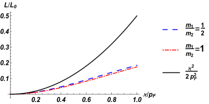
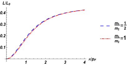
Figure 2: The Lorentz ratio in units of the Sommerfeld constant as a function of $\varkappa/p_{F}$, where $\varkappa$ is the inverse screening length defined by Eq. (18).

V.1 Lorentz ratio of WP₂

The Lorentz ratio measures the relative rates of relaxation of electrical and thermal currents, with $L=L_{0}$ indicating that the two rates are same. Recent experiments on a compensated metal WP₂Jaoui et al. (2018) found a very low Lorentz ratio ($L/L_{0}\approx 0.2$), which indicates that the electrical current is relaxed much slower than the thermal one. This low Lorentz ratio was observed in the temperature range where both $\rho$ and $T/\kappa$ scale as $T^{2}$, which suggests that the dominant scattering mechanism is electron-electron interaction. According to the discussion in the previous two sections, a low Lorentz ratio can occur if either the interaction is of a long-range type, or if the interaction is of a short-range type but intraband scattering is much stronger than interband one.

In the first scenario, the Lorentz ratio is parameterized by the average square of the scattering angle [See Eq. (57)] which, for the screened Coulomb potential translates into Eq. (58). In a multiband system

$$\varkappa^{2}=\frac{4e^{2}}{\pi\epsilon_{0}}\sum_{j}m_{j}p_{F,j},$$ (61)

where $m_{j}$ and $p_{F,j}$ are the effective mass and Fermi momentum of the $j\text{th}$ band, respectively. WP₂ has two electron pockets with masses $m_{\gamma}=0.87\,m_{0}$ and $m_{\delta}=0.99\,m_{0}$, and two hole pockets with masses $m_{\alpha}=1.67\,m_{0}$ and $m_{\beta}=0.89\,m_{0}$ (Ref. Gooth et al., 2018). The total number density of electrons (equal to that of holes) is $n\approx 2.5\times 10^{21}$cm^-3. According to the exact solution of the BEs (dashed and dashed-and-dotted lines in Fig. 2), the Lorentz ratio reaches the observed value of $0.2$ already at $\varkappa/p_{F}\approx 1$. With material parameters indicated above, we have $\varkappa/p_{F}\approx\sqrt{30.8/\epsilon_{0}}$, and the forward-scattering scenario can explain the experiment only if $\epsilon_{0}$ is quite large: $\epsilon_{0}\gtrsim 30$. Interestingly, this may be the case for WP₂. Indeed, although we are not aware of optical measurements on this material, an anomalously large value of $\epsilon_{\infty}$ (from $75$ to $91$, depending on orientation) have recently been reported for a cousin material WTe₂ (Ref. Frenzel et al., 2017), which is also a type-II Weyl semimetal. Since $\epsilon_{0}\geqslant\epsilon_{\infty}$, the condition $\epsilon_{0}\gtrsim 30$ is then satisfied within a good margin. Alternatively, a small Lorentz ratio can result from strong intraband scattering with short-range interaction. With comparable masses of electron and hole bands, the observed value of $L/L_{0}$ can be already achieved if $W/W^{11}=W/W^{22}\approx 0.4$, which is not unrealistic. Optical data for $\epsilon_{\infty}$ in WP₂ are obviously needed to discriminate between the forward- and isotropic-scattering scenarios.

VI Conclusions

In this paper, we calculated electrical and thermal conductivities of a clean compensated two-band metal with intercarrier interaction as the dominant scattering mechanism. From the theoretical standpoint, it is an attractive toy model which allows one to study both electrical and thermal transport properties, without invoking additional mechanisms of momentum relaxation. However, this model is also relevant to a large class of materials, i.e., metals and semimetals with even number of electrons per unit cell, which include many elemental metals, group V semimetals, graphite, parent states of iron-based superconductors, type-II Weyl semimetals, etc. To find the electrical and thermal conductivities, we solved exactly the system of coupled Boltzmann Equations, describing both inter- and intraband scattering, and analyzed the limiting cases of forward and isotropic scattering. We showed that the forward-scattering limit of the electrical conductivity can be obtained without knowing the exact solution: By assuming from the very beginning that the non-equilibrium part of the distribution function depends primarily on the directions of carriers’ momenta but not on their energies. For the thermal conductivity, the same procedure leads to a reasonable albeit not asymptotically exact approximation. We obtained the exact result for the Lorentz ratio and showed that it takes a particularly simple form, parameterized by the average square of the scattering angle, in the forward-scattering limit [cf. Eq. (57)]. We analyzed the Lorentz ratio of a type-II Weyl semimetal WP₂ and showed that a strong downward violation of the Wiedemann-Franz Law observed in this materialJaoui et al. (2018) can be explained within the forward-scattering model, provided that the high-frequency value of the dielectric constant in this material is sufficiently large.

Appendix A Exact solution of the coupled Boltzmann equations

In the Appendix we provide detailed derivations of the exact results for the electric resistivity and the thermal conductivity. To reiterate, “exact” here means that the results are valid for an arbitrary scattering probability but only for $T\ll\varepsilon_{F}$.

A.1 Electrical resistivity

To find the electrical resistivity of a two-band compensated metal, we start with the system of coupled Boltzmann equations, Eqs. (8a) and (8b). The non-equilibrium parts of the distribution functions are parameterized by Eq. (13). Defining dimensionless variables $x_{j}=\xi_{j}/T$ and $y=\omega/T$, where $\omega$ is the energy transfer in the scattering processes, we rewrite Eqs. (8a) and (8b) in the notations of Ref. Abrikosov and Khalatnikov, 1959 as

$$\frac{1}{m_{1}}n_{F}(x_{1})\left[1-n_{F}(x_{1})\right] = \frac{m_{1}m^{2}_{2}T^{2}}{8\pi^{4}}\int\frac{d\Omega}{4\pi}\frac{W(\theta,\phi)}{\cos(\theta/2)}\int dx_{2}\,dy\,\mathcal{Q}(x_{1},x_{2},y)$$ (62a)

$$\times\left[\frac{\varphi_{1}(x_{1})}{m_{1}}-\frac{\varphi_{2}(x_{2})}{m_{2}}\cos\theta-\frac{\varphi_{1}(x_{1}-y)}{m_{1}}\cos\Theta+\frac{\varphi_{2}(x_{2}+y)}{m_{2}}\cos\theta_{{\bf k}^{\prime}{\bf p}}\right],$$

$$\frac{1}{m_{2}}n_{F}(x_{2})\left[1-n_{F}(x_{2})\right] = \frac{m_{2}m^{2}_{1}T^{2}}{8\pi^{4}}\int\frac{d\Omega}{4\pi}\frac{W(\theta,\phi)}{\cos(\theta/2)}\int dx_{1}\,dy\,\mathcal{Q}(x_{1},x_{2},y)$$ (62b)

$$\times\left[\frac{\varphi_{2}(x_{2})}{m_{2}}-\frac{\varphi_{1}(x_{1})}{m_{1}}\cos\theta-\frac{\varphi_{2}(x_{2}+y)}{m_{2}}\cos\Theta+\frac{\varphi_{1}(x_{1}-y)}{m_{1}}\cos\theta_{{\bf p}^{\prime}{\bf k}}\right].$$

As in the main text, $\theta$ is the angle between the initial state momenta, ${\bf p}$ and ${\bf k}$, $\Theta$ is the scattering angle, $\phi$ is the angle between the planes formed by the initial and final momenta, respectively, $W(\theta,\phi)$ is the scattering probability, and $\cos\theta_{{\bf k}^{\prime}{\bf p}}=\cos\theta_{{\bf p}^{\prime}{\bf k}}=1+\cos\theta-\cos\Theta$, where $\theta_{{\bf m}{\bf n}}$ is the angle between vectors ${\bf n}$ and ${\bf m}$. Furthermore, $\mathcal{Q}$ represents the product of Fermi functions

$$\mathcal{Q}(x_{1},x_{2},y)=n_{F}(x_{1})n_{F}(x_{2})\left[1-n_{F}(x_{1}-y)\right]\left[1-n_{F}(x_{2}+y)\right],\,n_{F}(x)=1/\left(e^{x}+1\right).$$ (63)

Equations (62a) and (62b) can be further reduced to two coupled integral equations

$$1 = \tau^{-1}_{\rho 1}\frac{\pi^{2}+x_{1}^{2}}{2}\varphi_{1}(x_{1})-\lambda_{\rho}\tau^{-1}_{\rho 1}\int du\,\mathcal{F}(x_{1},u)\varphi_{1}(u)+(1-\lambda_{\rho})\tau^{-1}_{\rho 2}\int du\,\mathcal{F}(x_{1},u)\varphi_{2}(u),$$ (64a)

$$1 = \tau^{-1}_{\rho 2}\frac{\pi^{2}+x^{2}}{2}\varphi_{2}(x_{2})-\lambda_{\rho}\tau^{-1}_{\rho 2}\int du\,\mathcal{F}(x_{2},u)\varphi_{2}(u)+(1-\lambda_{\rho})\tau^{-1}_{\rho 1}\int du\,\mathcal{F}(x_{2},u)\varphi_{1}(u),$$ (64b)

where $\tau_{\rho 1,2}$ are given by Eq. (35a) and its analog with $1\leftrightarrow 2$, $\lambda_{\rho}$ is defined by Eq. (35b), and the kernel in the integrand reads

$$\mathcal{F}(x,u) = \frac{\cosh(x/2)}{\cosh(u/2)}\mathcal{G}(x-u),$$ (65a)

$$\mathcal{G}(x) = \frac{x}{2\sinh(x/2)}.$$ (65b)

To derive Eq. (64a) and (64b), we have used that

$$\int dx_{2}\int dy\mathcal{Q}(x_{1},x_{2},y)\varphi_{j}(x_{2}) = -n_{F}(x_{1})\left[1-n_{F}(x_{1})\right]\int du\mathcal{F}(x_{1},u)\varphi_{j}(u)$$ (66a)

$$\int dx_{2}\int dy\mathcal{Q}(x_{1},x_{2},y)\varphi_{j}(x_{1}-y) = n_{F}(x_{1})\left[1-n_{F}(x_{1})\right]\int du\mathcal{F}(x_{1},u)\varphi_{j}(u),$$ (66b)

$$\int dx_{2}\int dy\mathcal{Q}(x_{1},x_{2},y)\varphi_{j}(x_{2}+y) = n_{F}(x_{1})\left[1-n_{F}(x_{1})\right]\int du\mathcal{F}(x_{1},u)\varphi_{j}(u),$$ (66c)

with $$j=1,2$$.

Defining $\Phi_{j}(x)=\varphi_{j}(x)/(\tau_{\rho,j}\cosh\frac{x}{2})$, we arrive at

$$\frac{2}{\cosh(x_{1}/2)} = (\pi^{2}+x_{1}^{2})\Phi_{1}(x_{1})-2\int du\,\mathcal{G}(x_{1}-u)\left[\lambda_{\rho}\Phi_{1}(u)-(1-\lambda_{\rho})\Phi_{2}(u)\right],$$ (67a)

$$\frac{2}{\cosh(x_{2}/2)} = (\pi^{2}+x_{2}^{2})\Phi_{2}(x_{2})-2\int du\,\mathcal{G}(x_{2}-u)\left[\lambda_{\rho}\Phi_{2}(u)-(1-\lambda_{\rho})\Phi_{1}(u)\right].$$ (67b)

The integral equations can be reduced to the differential ones for Fourier transforms $\tilde{\Phi}_{j}(k)=\int dx\,\Phi_{j}(x)e^{ikx}$:

$$\frac{d^{2}\tilde{\Phi}_{1}(k)}{dk^{2}}+\pi^{2}\left[\frac{2\lambda_{\rho}}{\cosh^{2}(\pi k)}-1\right]\tilde{\Phi}_{1}(k)-\pi^{2}\frac{2(1-\lambda_{\rho})}{\cosh^{2}(\pi k)}\tilde{\Phi}_{2}(k) = -\frac{4\pi}{\cosh(\pi k)},$$ (68a)

$$\frac{d^{2}\tilde{\Phi}_{2}(k)}{dk^{2}}+\pi^{2}\left[\frac{2\lambda_{\rho}}{\cosh^{2}(\pi k)}-1\right]\tilde{\Phi}_{2}(k)-\pi^{2}\frac{2(1-\lambda_{\rho})}{\cosh^{2}(\pi k)}\tilde{\Phi}_{1}(k) = -\frac{4\pi}{\cosh(\pi k)}.$$ (68b)

Adding up the two equations above and introducing a variable $\zeta=\tanh(\pi k)$, we obtain an equation for $\tilde{\Phi}(k)=\tilde{\Phi}_{1}(k)+\tilde{\Phi}_{2}(k)$

$$\mathcal{L}\tilde{\Phi}(\zeta)+2(2\lambda_{\rho}-1)\tilde{\Phi}(\zeta)=-\frac{8}{\pi\sqrt{1-\zeta^{2}}},$$ (69)

where the linear differential operator $\mathcal{L}$ is given by

$$\mathcal{L}=\frac{d}{d\zeta}\left[(1-\zeta^{2})\frac{d}{d\zeta}\right]-\frac{1}{1-\zeta^{2}}.$$ (70)

The eigenfunctions of $\mathcal{L}$ are associated Legendre polynomials, $P^{1}_{l}(\zeta)$: $\mathcal{L}P^{1}_{l}(\zeta)=-l(l+1)P^{1}_{l}(\zeta)$, $l=1,2,3\dots$ Expanding $\tilde{\Phi}(\zeta)$ in series over $P^{1}_{l}(\zeta)$

$$\tilde{\Phi}(\zeta)=\sum_{l}c_{l}P^{1}_{l}(\zeta),$$ (71)

and using the orthogonality relation

$$\int^{1}_{-1}d\zeta P^{1}_{l}(\zeta)P^{1}_{m}(\zeta)=\frac{2l(l+1)}{2l+1}\delta_{lm}$$ (72)

and an identity

$$\int^{1}_{-1}d\zeta\frac{P^{1}_{l}(\zeta)}{\sqrt{1-\zeta^{2}}}=\Big{\{}\begin{array}[]{cc}-2,&\mbox{if $l$ is odd};\\ 0,&\mbox{if $l$ is even},\end{array}$$ (75)

we obtain Eq. (37) of the main text.

The electrical resistivity is given by

$$\rho = \frac{1}{ne^{2}}\left[\sum_{j=1,2}\frac{\tau_{\rho,j}}{m_{j}}\int dx\frac{\Phi_{j}(x)}{4\cosh(x/2)}\right]^{-1}=\frac{1}{ne^{2}}\left[\sum_{j=1,2}\frac{\tau_{\rho,j}}{m_{j}}\int dk\frac{\tilde{\Phi}_{j}(k)}{4\cosh(\pi k)}\right]^{-1}$$ (76)

$$= \frac{1}{ne^{2}}\frac{m^{2}_{1}m^{2}_{2}T^{2}}{2\pi^{4}}\Big{\langle}\frac{W(\theta,\phi)}{\cos(\theta/2)}\Big{\rangle}\left[\int dk\frac{\tilde{\Phi}(k)}{\cosh(\pi k)}\right]^{-1}=\frac{1}{ne^{2}}\frac{m^{2}_{1}m^{2}_{2}T^{2}}{2\pi^{4}}\Big{\langle}\frac{W(\theta,\phi)}{\cos(\theta/2)}\Big{\rangle}\left[\frac{1}{\pi}\int^{1}_{-1}d\zeta\frac{\tilde{\Phi}(\zeta)}{\sqrt{1-\zeta^{2}}}\right]^{-1}$$

$$= \frac{1}{ne^{2}}\frac{m^{2}_{1}m^{2}_{2}T^{2}}{8\pi^{2}}\Big{\langle}\frac{W(\theta,\phi)}{\cos(\theta/2)}\Big{\rangle}\left[\sum^{\infty}_{l=0}\frac{4l+3}{(l+1)(2l+1)}\,\frac{1}{(l+1)(2l+1)-(2\lambda_{\rho}-1)}\right]^{-1},$$

which reproduces the result in Eq. (38).

A.2 Thermal conductivity

In the same parametrization as in the previous section, Eqs. (LABEL:eq:BE_thermal_1) and (LABEL:eq:BE_thermal_2) in the presence of a thermal gradient read

$$\frac{1}{m_{1}}x_{1}\,n_{F}(x_{1})\left[1-n_{F}(x_{1})\right] = \frac{m^{3}_{1}T^{2}}{8\pi^{4}}\int\frac{d\Omega}{4\pi}\frac{W^{11}(\theta,\phi)}{\cos(\theta/2)}\int dx_{2}\,dy\,\mathcal{Q}(x_{1},x_{2},y)$$ (77a)

$$\times\frac{1}{m_{1}}\left[\psi_{1}(x_{1})+\psi_{1}(x_{2})\cos\theta-\psi_{1}(x_{1}-y)\cos\Theta-\psi_{1}(x_{2}+y)\cos\theta_{{\bf k}^{\prime}{\bf p}}\right]$$

$$+\frac{m_{1}m^{2}_{2}T^{2}}{8\pi^{4}}\int\frac{d\Omega}{4\pi}\frac{W(\theta,\phi)}{\cos(\theta/2)}\int dx_{2}\,dy\,\mathcal{Q}(x_{1},x_{2},y)$$

$$\times\left[\frac{\psi_{1}(x_{1})}{m_{1}}-\frac{\psi_{2}(x_{2})}{m_{2}}\cos\theta-\frac{\psi_{1}(x_{1}-y)}{m_{1}}\cos\Theta+\frac{\psi_{2}(x_{2}+y)}{m_{2}}\cos\theta_{{\bf k}^{\prime}{\bf p}}\right],$$

$$\frac{1}{m_{2}}x_{2}\,n_{F}(x_{2})\left[1-n_{F}(x_{2})\right] = \frac{m^{3}_{2}T^{2}}{16\pi^{4}}\int\frac{d\Omega}{4\pi}\frac{W^{22}(\theta,\phi)}{\cos(\theta/2)}\int dx_{1}\,dy\,\mathcal{Q}(x_{1},x_{2},y)$$ (77b)

$$\times\frac{1}{m_{2}}\left[\psi_{2}(x_{2})+\psi_{2}(x_{1})\cos\theta-\psi_{2}(x_{2}+y)\cos\Theta-\psi_{2}(x_{1}-y)\cos\theta_{{\bf p}^{\prime}{\bf k}}\right]$$

$$+\frac{m_{2}m^{2}_{1}T^{2}}{16\pi^{4}}\int\frac{d\Omega}{4\pi}\frac{W(\theta,\phi)}{\cos(\theta/2)}\int dx_{1}\,dy\,\mathcal{Q}(x_{1},x_{2},y)$$

$$\times\left[\frac{\psi_{2}(x_{2})}{m_{2}}-\frac{\psi_{1}(x_{1})}{m_{1}}\cos\theta-\frac{\psi_{2}(x_{2}+y)}{m_{2}}\cos\Theta+\frac{\psi_{1}(x_{1}-y)}{m_{1}}\cos\theta_{{\bf p}^{\prime}{\bf k}}\right].$$

Eqs. (77a) and (77b) can be further reduced to two coupled integral equations,

$$\tau_{\kappa 1}\,x_{1} = \frac{\pi^{2}+x_{1}^{2}}{2}\psi_{1}(x_{1})-\lambda_{\kappa 1}\int du\,\mathcal{F}(x_{1},u)\psi_{1}(u)+\beta_{\kappa 1}\int du\,\mathcal{F}(x_{1},u)\psi_{2}(u),$$ (78a)

$$\tau_{\kappa 2}\,x_{2} = \frac{\pi^{2}+x^{2}}{2}\psi_{2}(x_{2})-\lambda_{\kappa 2}\int du\,\mathcal{F}(x_{2},u)\psi_{2}(u)+\beta_{\kappa 2}\int du\,\mathcal{F}(x_{2},u)\psi_{1}(u),$$ (78b)

where parameters $\tau_{\kappa 1,2}$, $\lambda_{\kappa 1,2}$, and $\beta_{\kappa 1,2}$ are given by Eqs. (LABEL:tk2), (LABEL:lk1) and (35e), respectively, and their analogs with $1\leftrightarrow 2$, and kernels $\mathcal{F}(x,u)$ and $\mathcal{G}(x)$ are defined by Eqs. (65a) and (65b), respectively. Defining $\Psi_{j}(x)=\psi_{j}(x)/(\tau_{\kappa,j}\cosh\frac{x}{2})$, we arrive at

$$\frac{2x_{1}}{\cosh(x_{1}/2)} = (\pi^{2}+x_{1}^{2})\Psi_{1}(x_{1})-2\int du\,\mathcal{G}(x_{1}-u)\left[\lambda_{\kappa 1}\Psi_{1}(u)-\frac{\beta_{\kappa 1}\tau_{\kappa 2}}{\tau_{\kappa 1}}\Psi_{2}(u)\right],$$ (79a)

$$\frac{2x_{2}}{\cosh(x_{2}/2)} = (\pi^{2}+x_{2}^{2})\Psi_{2}(x_{2})-2\int du\,\mathcal{G}(x_{2}-u)\left[\lambda_{\kappa 2}\Psi_{2}(u)-\frac{\beta_{\kappa 2}\tau_{\kappa 1}}{\tau_{\kappa 2}}\Psi_{1}(u)\right].$$ (79b)

After a Fourier transformation, $\tilde{\Psi}_{j}(k)=\int dx\,\Psi_{j}(x)e^{ikx}$, Eqs. (79a) and (79b) become

$$\mathcal{L}\tilde{\Psi}_{1}(\zeta)+2\lambda_{\kappa 1}\tilde{\Psi}_{1}(\zeta)-2\frac{\beta_{\kappa 1}\tau_{\kappa 2}}{\tau_{\kappa 1}}\tilde{\Psi}_{2}(\zeta) = -i\frac{4\zeta}{\sqrt{1-\zeta^{2}}},$$ (80a)

$$\mathcal{L}\tilde{\Psi}_{2}(\zeta)+2\lambda_{\kappa 2}\tilde{\Psi}_{2}(\zeta)-2\frac{\beta_{\kappa 2}\tau_{\kappa 1}}{\tau_{\kappa 2}}\tilde{\Psi}_{1}(\zeta) = -i\frac{4\zeta}{\sqrt{1-\zeta^{2}}}.$$ (80b)

Expanding $\tilde{\Psi}_{\kappa 1}(\zeta)$ and $\tilde{\Psi}_{\kappa 2}(\zeta)$ in series of the associated Legendre polynomial $P^{1}_{l}(\zeta)$,

$$\tilde{\Psi}_{1}(\zeta)=i\sum_{n}a_{l}P^{1}_{l}(\zeta),\,\tilde{\Psi}_{2}(\zeta)=i\sum_{l}b_{l}P^{1}_{l}(\zeta),$$ (81)

we then obtain

$$\left[l(l+1)-2\lambda_{\kappa 1}\right]a_{l}+\frac{2\beta_{\kappa 1}\tau_{\kappa 2}}{\tau_{\kappa 1}}b_{l} = \frac{2(2l+1)}{l(l+1)}\int^{1}_{-1}d\zeta\frac{\zeta P^{1}_{l}(\zeta)}{\sqrt{1-\zeta^{2}}},$$ (82a)

$$\frac{2\beta_{\kappa 2}\tau_{\kappa 1}}{\tau_{\kappa 2}}a_{l}+\left[l(l+1)-2\lambda_{\kappa 2}\right]b_{l} = \frac{2(2l+1)}{l(l+1)}\int^{1}_{-1}d\zeta\frac{\zeta P^{1}_{l}(\zeta)}{\sqrt{1-\zeta^{2}}}.$$ (82b)

Solving for $a_{l}$ and $b_{l}$, we find

$$a_{l} = -\frac{l(l+1)-2\lambda_{\kappa 2}-2\beta_{\kappa 1}\tau_{\kappa 2}/\tau_{\kappa 1}}{\left[l(l+1)-2\lambda_{\kappa 1}\right]\left[l(l+1)-2\lambda_{\kappa 2}\right]-4\beta_{\kappa 1}\beta_{\kappa 2}}\,\frac{4(2l+1)}{l(l+1)},$$ (83a)

$$b_{l} = -\frac{l(l+1)-2\lambda_{\kappa 1}-2\beta_{\kappa 2}\tau_{\kappa 1}/\tau_{\kappa 2}}{\left[l(l+1)-2\lambda_{\kappa 1}\right]\left[l(l+1)-2\lambda_{\kappa 2}\right]-4\beta_{\kappa 1}\beta_{\kappa 2}}\,\frac{4(2l+1)}{l(l+1)},$$ (83b)

where we have again used Eq. (72) and another identity

$$\int^{1}_{-1}d\zeta\frac{\zeta P^{1}_{l}(\zeta)}{\sqrt{1-\zeta^{2}}}=\Big{\{}\begin{array}[]{cc}-2,&\mbox{if $l$ is even};\\ 0,&\mbox{if $l$ is odd}.\end{array}$$ (86)

Substituting $a_{l}$ and $b_{l}$ into Eq. (81), we reproduce Eqs. (41a) and (41b) of the main text.

The thermal conductivity is found as

$$\kappa = nT\left[\sum_{j=1,2}\frac{\tau_{\kappa,j}}{m_{j}}\int dx\frac{x}{4\cosh(x/2)}\Psi_{j}(x)\right]=-i\pi nT\left[\sum_{j=1,2}\frac{\tau_{\kappa,j}}{m_{j}}\int dk\frac{\sinh(\pi k)}{4\cosh^{2}(\pi k)}\tilde{\Psi}_{j}(k)\right]$$ (87)

$$= -i\frac{nT}{4}\left[\sum_{j=1,2}\frac{\tau_{\kappa,j}}{m_{j}}\int^{1}_{-1}d\zeta\frac{\zeta\tilde{\Psi}_{j}(\zeta)}{\sqrt{1-\zeta^{2}}}\right]$$

$$= \frac{4\pi^{4}n}{m^{2}_{1}T}\frac{1}{m^{2}_{1}\Big{\langle}W^{11}(\theta,\phi)/\cos\frac{\theta}{2}\Big{\rangle}+m^{2}_{2}\Big{\langle}W(\theta,\phi)/\cos\frac{\theta}{2}\Big{\rangle}}\times$$

$$\sum^{\infty}_{l=0}\frac{4l+5}{(l+1)(2l+3)}\frac{(l+1)(2l+3)-\lambda_{\kappa 2}-\beta_{\kappa 1}\tau_{\kappa 2}/\tau_{\kappa 1}}{\left[(l+1)(2l+3)-\lambda_{\kappa 1}\right]\left[(l+1)(2l+3)-\lambda_{\kappa 2}\right]-\beta_{\kappa 1}\beta_{\kappa 2}}$$

$$+\frac{4\pi^{4}n}{m^{2}_{2}T}\frac{1}{m^{2}_{2}\Big{\langle}W^{22}(\theta,\phi)/\cos\frac{\theta}{2}\Big{\rangle}+m^{2}_{1}\Big{\langle}W(\theta,\phi)/\cos\frac{\theta}{2}\Big{\rangle}}\times$$

$$\sum^{\infty}_{l=0}\frac{4l+5}{(l+1)(2l+3)}\frac{(l+1)(2l+3)-\lambda_{\kappa 1}-\beta_{\kappa 2}\tau_{\kappa 1}/\tau_{\kappa 2}}{\left[(l+1)(2l+3)-\lambda_{\kappa 1}\right]\left[(l+1)(2l+3)-\lambda_{\kappa 2}\right]-\beta_{\kappa 1}\beta_{\kappa 2}},$$

which reproduces Eq. (42) in the main text.

References

• Ziman (2001) J. Ziman, Electrons and Phonons (Oxford University Press, Oxford, 2001).
• Abrikosov (1988) A. A. Abrikosov, Fundamentals of the Theory of Metals, Fundamentals of the Theory of Metals (North-Holland, Amsterdam, 1988).
• Lifshitz and Pitaevskii (1981) E. M. Lifshitz and L. P. Pitaevskii, Physical Kinetics, Course of Theoretical Physics, v. X (Butterworth-Heinemann, Burlington, 1981).
• Note (1) Historically, the WFL was observed first in the regime of quasielastic electron-phonon scatteringFranz and Wiedemann (1853) because cryogenic technologies were not available in 1853.
• White and Tainsh (1960) G. K. White and R. J. Tainsh, Phys. Rev. 119, 1869 (1960).
• Zhang et al. (2000) Y. Zhang, N. P. Ong, Z. A. Xu, K. Krishana, R. Gagnon,  and L. Taillefer, Phys. Rev. Lett. 84, 2219 (2000).
• Yao et al. (2017) M. Yao, M. Zebarjadi,  and C. P. Opeil, J. Appl. Phys. 122, 135111 (2017).
• Lussier et al. (1994) B. Lussier, B. Ellman,  and L. Taillefer, Phys. Rev. Lett. 73, 3294 (1994).
• Paglione et al. (2005) J. Paglione, M. A. Tanatar, D. G. Hawthorn, R. W. Hill, F. Ronning, M. Sutherland, L. Taillefer, C. Petrovic,  and P. C. Canfield, Phys. Rev. Lett. 94, 216602 (2005).
• Tanatar et al. (2007) M. A. Tanatar, J. Paglione, C. Petrovic,  and L. Taillefer, Science 316, 1320 (2007).
• Dong et al. (2013) J. K. Dong, Y. Tokiwa, S. L. Bud’ko, P. C. Canfield,  and P. Gegenwart, Phys. Rev. Lett. 110, 176402 (2013).
• Machida et al. (2013) Y. Machida, K. Tomokuni, K. Izawa, G. Lapertot, G. Knebel, J.-P. Brison,  and J. Flouquet, Phys. Rev. Lett. 110, 236402 (2013).
• Ronning et al. (2006) F. Ronning, R. W. Hill, M. Sutherland, D. G. Hawthorn, M. A. Tanatar, J. Paglione, L. Taillefer, M. J. Graf, R. S. Perry, Y. Maeno,  and A. P. Mackenzie, Phys. Rev. Lett. 97, 067005 (2006).
• Gooth et al. (2018) J. Gooth, F. Menges, N. Kumar, V. Süß, C. Shekhar, Y. Sun, U. Drechsler, R. Zierold, C. Felser,  and B. Gotsmann, Nat. Commun. 9, 4093 (2018).
• Jaoui et al. (2018) A. Jaoui, B. Fauqué, C. W. Rischau, A. Subedi, C. Fu, J. Gooth, N. Kumar, V. Süß, D. L. Maslov, C. Felser,  and K. Behnia, npj Quantum Materials 3, 64 (2018).
• Note (2) A drastic upward violation of the WFL is observed in graphene at the charge neutrality pointCrossno et al. (2016) and is understood as arising from the weakness of electron-hole generation-recombination processes, which control the thermal conductivity of graphene Müller et al. (2008); Foster and Aleiner (2009); Crossno et al. (2016).
• Maslov et al. (2011) D. L. Maslov, V. I. Yudson,  and A. V. Chubukov, Phys. Rev. Lett. 106, 106403 (2011).
• Pal et al. (2012) H. K. Pal, V. I. Yudson,  and D. L. Maslov, Lith. J. Phys. 52, 142 (2012).
• Maslov and Chubukov (2017) D. L. Maslov and A. V. Chubukov, Rep. Prog. Phys. 80, 026503 (2017).
• Baber (1937) W. G. Baber, Proc. Royal Soc. London A 158, 383 (1937).
• Fawcett and Reed (1963) E. Fawcett and W. A. Reed, Phys. Rev. 131, 2463 (1963).
• Stewart (2011) G. R. Stewart, Rev. Mod. Phys. 83, 1589 (2011).
• Soluyanov et al. (2015) A. A. Soluyanov, D. Gresch, Z. Wang, Q. Wu, M. Troyer, X. Dai,  and B. A. Bernevig, Nature 527, 495 (2015).
• Razzoli et al. (2018) E. Razzoli, B. Zwartsenberg, M. Michiardi, F. Boschini, R. P. Day, I. S. Elfimov, J. D. Denlinger, V. Süss, C. Felser,  and A. Damascelli, Phys. Rev. B 97, 201103 (2018).
• (25) For metals with open Fermi surfaces, such as WP2, “compensation” can be understood as the equality of volumes of electron and hole parts of the Fermi surface within the first Brillouin zoneAlekseevskiĭ et al. (1961).
• Kumar et al. (2017) N. Kumar, Y. Sun, N. Xu, K. Manna, M. Yao, V. Süss, I. Leermakers, O. Young, T. Förster, M. Schmidt, H. Borrmann, B. Yan, U. Zeitler, M. Shi, C. Felser,  and C. Shekhar, Nat. Commun. 8, 1642 (2017).
• Fauqué et al. (2018) B. Fauqué, X. Yang, W. Tabis, M. Shen, Z. Zhu, C. Proust, Y. Fuseya,  and K. Behnia, Phys. Rev. Materials 2, 114201 (2018).
• Gurzhi (1968) R. N. Gurzhi, Phys. Usp. 11, 255 (1968).
• Coulter et al. (2018) J. Coulter, R. Sundararaman,  and P. Narang, Phys. Rev. B 98, 115130 (2018).
• Abrikosov and Khalatnikov (1959) A. A. Abrikosov and I. M. Khalatnikov, Rep. Prog. Phys. 22, 329 (1959).
• Brooker and Sykes (1968) G. A. Brooker and J. Sykes, Phys. Rev. Lett. 21, 279 (1968).
• Jensen et al. (1968) H. H. Jensen, H. Smith,  and J. Wilkins, Phys. Lett. A 27, 532 (1968).
• Sykes and Brooker (1970) J. Sykes and G. Brooker, Ann. Phys. 56, 1 (1970).
• E. M. Lifshitz and L. P. Pitaevski (1980) E. M. Lifshitz and L. P. Pitaevski, Statistical Physics, Part II, Course of Theoretical Physics, v. IX (Pergamon Press, New York, 1980).
• D. Pines and P. Nozières (1966) D. Pines and P. Nozières, The Theory of Quantum Liquids. v. I: Normal Fermi Liquids (Benjamin, New York, 1966).
• Shekhter and Finkel’stein (2006) A. Shekhter and A. M. Finkel’stein, Proc. Natl. Acad. Sci. USA 103, 15765 (2006).
• Chubukov and Maslov (2007) A. V. Chubukov and D. L. Maslov, Phys. Rev. B 76, 165111 (2007).
• (38) D. S. Novikov, arXiv:cond-mat/0603184 .
• Note (3) Strictly speaking, the even part of $\psi_{j}$ is also to be found as it ensures the boundary condition of no macroscopic current. However, the even part of $\psi_{j}$ leads to a contribution to thermal conductivity which is smaller by a factor of $(T/\varepsilon_{F})^{2}$ compared to that from the odd part Abrikosov (1988).
• Lyakhov and Mishchenko (2003) A. O. Lyakhov and E. G. Mishchenko, Phys. Rev. B 67, 041304 (2003).
• Maldague and Kukkonen (1979) P. F. Maldague and C. A. Kukkonen, Phys. Rev. B 19, 6172 (1979).
• Note (4) Although our model has only two pockets, additional pockets can be incorporated by replacing $m_{1}$ and $m_{2}$ by properly averaged masses. Since the masses cancel out in $L/L_{0}$, a particular way of averaging does not matter.
• Frenzel et al. (2017) A. J. Frenzel, C. C. Homes, Q. D. Gibson, Y. M. Shao, K. W. Post, A. Charnukha, R. J. Cava,  and D. N. Basov, Phys. Rev. B 95, 245140 (2017).
• Franz and Wiedemann (1853) R. Franz and G. Wiedemann, Ann. der Physik 165, 497 (1853).
• Crossno et al. (2016) J. Crossno, J. K. Shi, K. Wang, X. Liu, A. Harzheim, A. Lucas, S. Sachdev, P. Kim, T. Taniguchi, K. Watanabe, T. A. Ohki,  and K. C. Fong, Science 351, 1058 (2016).
• Müller et al. (2008) M. Müller, L. Fritz,  and S. Sachdev, Phys. Rev. B 78, 115406 (2008).
• Foster and Aleiner (2009) M. S. Foster and I. L. Aleiner, Phys. Rev. B 79, 085415 (2009).
• Alekseevskiĭ et al. (1961) N. Alekseevskiĭ, Y. P. Gaĭdukov, I. M. Lifshitz,  and V. G. Peschanskiĭ, Sov. Phys.–JETP 12, 837 (1961).