A Partition Theorem for a Randomly Selected Large Population

Abstract.

We state and prove a theorem on the partitioning of a randomly selected large population into stationary and non-stationary components by using a property of stationary population identity. Applications of this theorem for practical purposes is summarized at the end.

1. Stationary Population

Stationary population assumptions and related mathematical formulations were of interest to Edmond Halley an astronomer to influential mathematician Leonhard Euler to twentieth-century famous theoretical population biologist Alfred Lotka. A population is said to be stationary if it has a zero growth rate and a constant population age-structure, and if not, the population is said to be non-stationary. Lotka associated his theory of stationary populations with the average rate at which a woman in her lifetime will be replaced by a girl (which we call the net reproduction rate). In fact, Lotka [12, 13] logically argued that the rate of natural growth, $r,$ of a population will be zero in (1.1) when the net reproduction rate of the population, $R_{0}$ will be equal to one (the notation of $R_{0}$ was introduced by Lotka). The relation between $r$ and $R_{0}$ is given by

(1.1) $$r=\frac{\ln(R_{0})}{L},$$

where $L$ is the length of the generation of a population and is expressed as,

(1.2) $$L=\frac{1}{R_{0}}\intop_{0}^{\infty}xa(x)s(x)dx,$$

where $a(x)$ is the age-specific fertility rates of women of age $x$ to give births to girl babies and $s(x)$ is the survival probability function for the women to live up to the age $x$.

We define below stationary population identity (SPI) or the Life Table Identity for a discrete population as given in [9].

Definition 1.

Stationary Population identity (SPI) or the Life Table Identity: Let $X$ be the set of elements representing proportion of population at each age of a stationary population or a life table population and $Y$ be the set of elements representing the remaining time units to be lived at each age of this stationary population. We say SPI holds if $X=Y.$

Let $A=\{0,a_{1},a_{2},...,\omega\}$ be the discrete set of ages in the population of a life table. Here $\omega$ is the maximum age in the population life table. The SPI holds for a life table means, in a life table, the proportion of population at age $x$ (say, $f_{1}(x)$) for $x\in A$ is equal to the proportion, (say, $f_{2}(x)$) of the population who will live $x-$years, i.e. $f_{1}(x)=f_{2}(x)$$\>\forall\>x\in A.$

This identity was theoretically demonstrated in partitioning large populations [9]. This identity was frequently referred also as life table identity in the mathematical population biology and demography literature. Such identities are found in various published literature, for example, see [1, 2, 3, 4, 5]. There were other related equalities in stationary populations which suggest an average of a stationary population is equal to the average expectation of remaining life (for continuous versions) [10, 11]. Although Lotka and Cox in their respective works have chosen continuous frameworks, in this article the population ages are treated on a discrete framework.

In this article, we have stated and proved a novel theorem that states a criterion to partition a randomly selected population into stationary and non-stationary components under a large discrete population model framework. The criterion is to compare $f_{1}(x)$ and $f_{1}(x)$ and see if they are identical. Instead of the life table population, the theorem suggests comparing the fraction population at each age of the actual population at a time point with the fraction of the populations that have remaining ages in the corresponding life table population constructed at the same time. In general, we do not see often stationary populations, except in life tables. But a careful investigation at any large population data suggests that a sub-population of a population could obey the properties of a stationary population. Now, through the partition theorem that is proved in this article, it becomes easier to understand the stationary component of large populations instantly without being dependent on the measures like NRR (net reproduction rate). Moreover, satisfying the theorem indicates certainly one can find if any component of a large population is stationary.

2. Partition Theorem and Proof

Theorem 2.

Stationary Population Identity (SPI) partitions a randomly selected large population into stationary and non-stationary components.

Proof.

Let $P(t)$ be the randomly selected large population at time t and $P_{x}(t)$ be its sub-population who are at age $x$, where $P(t)$ can be expressed as $P(t)=\int_{0}^{\omega}P_{x}(t)dx$ or $P(t)=\Sigma_{x=0}^{\omega}P_{x}(t)$ depending upon whether $x$ is measured as continuous or discrete ($\omega$ is the maximum age of life). In the current proof, we considered P as a summation over discrete ages. Let $g_{1}(x)=\frac{P_{x}(t)}{P(t)}$ for all $x\in A$. We do not know whether $P(t)$ is a stationary population or not. Stationary component of $P(t)$ (say, $M(t)$), we define as, a sub-collection of various aged individuals of $P(t)$ who form a sub-population and satisfy $g_{1}(y)=f_{2}(y)$ for a set of $y$ values in $A,$ where $f_{2}(y)$, as defined in the previous section, the proportion of the population who will have $y-$years remaining to live. Non-stationary component of $P(t)$ (say, $N(t)$), we define as, a sub-collection of $P(t)$ who are of age $z$ and satisfy $g_{1}(z)\neq f_{2}(z)$ for a set of all $z$ values in $A$. The sum of the sizes of $M(t)$ and $N(t)$ will be $P(t).$

Let us choose all individuals at age $y$ in $P(t)$ and consider

(2.1) $$g_{1}(y)=\frac{P_{y}(t)}{P(t)}.$$

From the life table constructed for the population $P(t)$ (Assumably for the single ages of the set $A$), we can obtain the proportion of population who have expected remaining years within $[A,$ and compare the proportion of population at each age $x\in A$ in $P(t).$ Note that, a life table is a mathematical model to synthetically demonstrate the age-specific death rates of a population and to compute remaining average years to live at each age in $A$. There are several books available to understand details of life table constructions, for example, see [6, 7, 8]. That is, we will compare $g_{1}(y)$ with another proportion $f_{2}(x)$ $\forall x\in A,$ where

(2.2) $$f_{2}(x)=\frac{L_{x}(t)}{L(t)}.$$

Here $L_{x}(t)$ is the life table population at time $t$ whose remaining years to live is $x$ and $L(t)$ is total life table population at $t$. First, we match $\frac{P_{y_{1}}(t)}{P(t)}$ for a given $y_{1}\in A$ in (2.1) with $\frac{L_{x}(t)}{L(t)}$ for each $x\in A.$ If $\frac{P_{y_{1}}(t)}{P(t)}$ is equal to $\frac{L_{x}(t)}{L(t)}$ for some $x,$ then we call the corresponding life table proportion of the population as $\frac{L_{y_{1}}(t)}{L(t)}$ $(say,$$f_{2}(y_{1})$). That is, $\frac{L_{y_{1}}(t)}{L(t)}$ is the proportion of life table sub-population who have $y_{1}$ years to live. This follows,

(2.3) $$g_{1}(y_{1})=\frac{P_{y_{1}}(t)}{P(t)}=\frac{L_{y_{1}}(t)}{L(t)}=f_{2}(y_{1}).$$

Suppose $\frac{P_{y_{1}}(t)}{P(t)}$ does not equal to any of the proportions $\frac{L_{x}(t)}{L(t)}$ for $x\in[0,\omega),$ then we denote $y_{1}$ in (2.3) by $z_{1}$ and write this situation as $g_{1}(z_{1})\neq f_{2}(z_{1}).$ That is, for any of the proportions $\frac{L_{x}(t)}{L(t)}$ for $x\in[0,\omega),$ the remaining years to live is not equal to $y_{1}.$

We will continue matching $\frac{P_{y_{2}}(t)}{P(t)}$ for some $y_{2}\neq y_{1}$ and $y_{2}\in[0,\omega)$ with $\frac{L_{x}(t)}{L(t)}$ for each $x\in A$ except for $x=y_{1}.$ If there is a value of $\frac{L_{x}(t)}{L(t)}$ that equals $\frac{P_{y_{2}}(t)}{P(t)},$ we call the corresponding proportion in life table population as $\frac{L_{y_{2}}(t)}{L(t)}$ (say, $f_{2}(y)$). $\frac{L_{y_{2}}(t)}{L(t)}$ is the proportion of life table sub-population who have $y_{2}$ years to live. That is,

(2.4) $$g_{1}(y_{2})=\frac{P_{y_{2}}(t)}{P(t)}=\frac{L_{y_{2}}(t)}{L(t)}=f_{2}(y_{2}).$$

Suppose $\frac{P_{y_{2}}(t)}{P(t)}$ does not equal to any of the proportions $\frac{L_{x}(t)}{L(t)}$ for $x\in A$, then we denote $y_{2}$ in (2.4) by $z_{2}$ (if $z_{1}$ already arises in an earlier situation such that $g_{1}(z_{1})\neq f_{2}(z_{1}))$, then we write $g_{1}(z_{2})\neq f_{2}(z_{2}).$ However, if $g_{1}(y_{1})=f_{2}(y_{1})$ exists but $\frac{P_{y_{2}}(t)}{P(t)}\neq\frac{L_{x}(t)}{L(t)}$ $\forall x\in A$, then $y_{2}$ in (2.4) we denote as $z_{1}$ and write $g_{1}(z_{1})\neq f_{2}(z_{1}).$

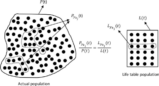
Figure 2.1. proportions of population in actual and in life table. $P_{y_{k_{j}}}(t)$ be its sub-population who are at age $y_{k_{j}}$, where $P(t)$ is the total actual population and $L_{y_{k_{j}}}(t)$ is the life table population at time $t$ whose remaining years to live is $y_{k_{j}}$ and $L(t)$ is total life table population at $t$.

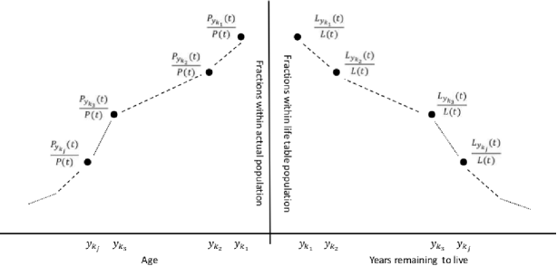
Figure 2.2. Stationary component of a randomly selected large population. proportional sub-populations at ages $y_{k_{1}},y_{k_{2}},...$ out of actual total population are identical with proportional life table sub-populations who have remaining years $y_{k_{1}},y_{k_{2}},...$.

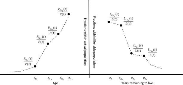
Figure 2.3. Non-stationary component of a randomly selected large population. proportional sub-populations at ages $z_{k_{1}},z_{k_{2}},...$ out of actual total population are not identical with any of the life table proportional sub-populations whose remaining years are $z_{k_{1}},z_{k_{2}},...$

Similarly, for a randomly selected age $y_{i}\in A$, the proportion $\frac{P_{y_{i}}(t)}{P(t)}$ (i.e. $g_{1}(y_{i})$) is matched with the proportion $\frac{L_{x}(t)}{L(t)}$ $\forall x\in A.$ If there is a value of $\frac{P_{y_{i}}(t)}{P(t)}$ that matches with $\frac{L_{x}(t)}{L(t)}$ then we denote it by $f_{2}(y_{i}),$ otherwise we denote it by $f_{2}(z_{i})$ (if previous $z$ value in the order of unmatched proportions was denoted as $z_{i-1}$ for $i=2,3,...$). Through this procedure we will match for all the values of $y_{i}\in A,$ and decide whether or not $g_{1}(y_{i})$ is equal to the $f_{2}(y_{i}).$ The criteria is, for an age $y_{i}$ in a randomly selected large population (actual population), if the value of the proportion $\frac{P_{y_{i}}(t)}{P(t)}$ is equal to any of the life table sub-population proportions $\frac{L_{x}(t)}{L(t)}$ $\forall x\in A$ whose remaining years to live is exactly $y_{i},$ then, $g_{1}(y_{i})=f_{2}(y_{i}).$

Existence of two sets $\{y_{k_{j}}\}$ and $\{z_{k_{j}}\}:$

In general, at each age $x\in A$, we can check whether

(2.5) $$\frac{P_{x}(t)}{P(t)}=\frac{L_{x}(t)}{L(t)}\text{ holds}$$

or

(2.6) $$\frac{P_{x}(t)}{P(t)}\neq\frac{L_{x}(t)}{L(t)}\text{ holds.}$$

Suppose we start this procedure from age $0.$ At $x=0$, either (2.5) holds or (2.6) holds but not both. If (2.5) holds then, let us denote $y_{k_{1}}$ for $0$, or if (2.6) holds then, let us denote $z_{k_{1}}$ for $0$. Hence, at age $0$ one of the $y_{k_{1}}$ or $z_{k_{1}}$ exists, and

(2.7) $$\left\{y_{k_{1}}\right\}\cup\left\{z_{k_{1}}\right\}=\left\{0\right\}$$

Now, let us consider age $a_{1}>0$ for $a_{1}\in A$. At age $x=a_{1}$, either (2.5) holds or (2.6) holds but not both. If (2.5) holds at $x=a_{1}$, and $y_{k_{1}}$ exists, then let us denote $y_{k_{2}}$ for $a_{1}$. If (2.5) holds at $x=a_{1}$ and $z_{k_{1}}$ exists, then let us denote $y_{k_{1}}$ for $a_{1}$. If (2.6) holds at $x=a_{1}$ and $y_{k_{1}}$ exist, then let us denote $z_{k_{1}}$ for $a_{1}$. If (2.6) is true at $x=a_{1}$ and $z_{k_{1}}$ exists, then let us denote $z_{k_{2}}$ for $a_{1}$. From the arguments constructed so far, we have shown the existence of one of the following sets:

(2.8) $$\left\{\{y_{k_{1}},y_{k_{2}}\},\{z_{k_{1}},y_{k_{1}}\},\{y_{k_{1}},z_{k_{1}}\},\{z_{k_{1}},z_{k_{2}}\}\right\}$$

The union of all the elements of the set (2.8) is

(2.9) $$\left\{\{y_{k_{1}},y_{k_{2}}\}\cup\{z_{k_{1}},y_{k_{1}}\}\cup\{y_{k_{1}},z_{k_{1}}\}\cup\{z_{k_{1}},z_{k_{2}}\}\right\}=\left\{0,a_{1}\right\}.$$

Now, let us consider age $a_{2}$ for $a_{2}>a_{1}>0$ and $a_{2}\in A$. At age $x=a_{2}$, either (2.5) holds or (2.6) holds but not both.

Suppose (2.5) holds at $x=a_{2}$. For $x=0$ and $x=a_{1}$, there is a possibility of occurrence of one of the four sets of (2.8) . All possible combinatorics of $x$ values are explained below:

$(i)$ (2.5) holds at $x=a_{2}$ and $\left\{y_{k_{1}},y_{k_{2}}\right\}$ exists, then let us denote $y_{k_{3}}$ for $a_{2}$.

$(ii)$ (2.5) holds at $x=a_{2}$ and $\{z_{k_{1}},y_{k_{1}}\}$ exists, then let us denote $y_{k_{2}}$ for $a_{2}$.

$(iii)$ (2.5) holds at $x=a_{2}$ and $\{y_{k_{1}},z_{k_{1}}\}$ exists, then let us denote $y_{k_{2}}$ for $a_{2}$.

$(iv)$ (2.5) holds at $x=a_{2}$ and $\{z_{k_{1}},z_{k_{2}}\}$ exists, then let us denote $y_{k_{1}}$ for $a_{2}$.

Suppose (2.6) holds at $x=a_{2}$. For $x=0$ and $x=a_{1}$, there is a possibility of occurrence of one of the four sets of (2.8). All possible combinatorics of $x$ values are explained below:

$(v)$ (2.6) holds at $x=a_{2}$ and $\left\{y_{k_{1}},y_{k_{2}}\right\}$ exists, then let us denote $z_{k_{1}}$ for $a_{2}$.

$(vi)$ (2.6) holds at $x=a_{2}$ and $\{z_{k_{1}},y_{k_{1}}\}$ exists, then let us denote $z_{k_{2}}$ for $a_{2}$.

$(vii)$ (2.6) holds at $x=a_{2}$ and $\{y_{k_{1}},z_{k_{1}}\}$ exists, then let us denote $z_{k_{2}}$ for $a_{2}$.

$(viii)$ (2.6) holds at $x=a_{2}$ and $\{z_{k_{1}},z_{k_{2}}\}$ exists, then let us denote $z_{k_{3}}$ for $a_{2}$.

Through $(i)$ to $(viii)$ we have shown the existence of one of the following sets:

(2.10) $$\left\{\begin{array}[]{c}\{y_{k_{1}},y_{k_{2}},y_{k_{3}}\},\{z_{k_{1}},y_{k_{1}},y_{k_{2}}\},\{y_{k_{1}},z_{k_{1}},y_{k_{2}}\},\{z_{k_{1}},z_{k_{2}},y_{k_{1}}\}\\ \{y_{k_{1}},y_{k_{2}},z_{k_{1}}\},\{z_{k_{1}},y_{k_{1}},z_{k_{2}}\},\{y_{k_{1}},z_{k_{1}},z_{k_{2}}\},\{z_{k_{1}},z_{k_{2}},z_{k_{3}}\}\end{array}\right\}$$

The union of all the elements (i.e. $2^{3}$ number of sets) of the set (2.10) is

(2.11) $$\left\{0,a_{1},a_{2}\right\}.$$

The number of possible sets at age $x=a_{3}$ once we construct similar to the previous arguments would be double the number of sets of (2.10), which is $2^{4}$ number of sets. These $2^{4}$ are given below:

(2.12) $$\left\{\begin{array}[]{c}\{y_{k_{1}},y_{k_{2}},y_{k_{3}},y_{k_{4}}\},\{z_{k_{1}},y_{k_{1}},y_{k_{2}},y_{k_{3}}\},\{y_{k_{1}},z_{k_{1}},y_{k_{2}},y_{k_{3}}\},\{z_{k_{1}},z_{k_{2}},y_{k_{1}},y_{k_{2}}\}\\ \{y_{k_{1}},y_{k_{2}},z_{k_{1}},y_{k_{3}}\},\{z_{k_{1}},y_{k_{1}},z_{k_{2}},y_{k_{2}}\},\{y_{k_{1}},z_{k_{1}},z_{k_{2}},y_{k_{2}}\},\{z_{k_{1}},z_{k_{2}},z_{k_{3}},y_{k_{1}}\}\\ \{y_{k_{1}},y_{k_{2}},y_{k_{3}},z_{k_{1}}\},\{z_{k_{1}},y_{k_{1}},y_{k_{2}},z_{k_{2}}\},\{y_{k_{1}},z_{k_{1}},y_{k_{2}},z_{k_{2}}\},\{z_{k_{1}},z_{k_{2}},y_{k_{1}},z_{k_{3}}\}\\ \{y_{k_{1}},y_{k_{2}},z_{k_{1}},z_{k_{2}}\},\{z_{k_{1}},y_{k_{1}},z_{k_{2}},z_{k_{3}}\},\{y_{k_{1}},z_{k_{1}},z_{k_{2}},z_{k_{3}}\},\{z_{k_{1}},z_{k_{2}},z_{k_{3}},z_{k_{4}}\}\end{array}\right\}$$

The union of $2^{4}$ sets in (2.12) is

$$\left\{0,a_{1},a_{2},a_{3}\right\}.$$

Note that the elements of (2.12) are drawn from the set

$$\{y_{k_{1}},y_{k_{2}},y_{k_{3}},y_{k_{4}},z_{k_{1}},z_{k_{2}},z_{k_{3}},z_{k_{4}}\}$$

which is of size $2.4=8.$

In a similar way, by the induction, the number of possible sets at age $x=a_{j}$ for $a_{j}>a_{j-1}>...>a_{1}>a_{0}$ would be $2^{j+1}$. Each of the set in the collection of $2^{j+1}$ will be of size $j+1$. These $j+1$ elements are drawn from the unique combinations of $2j+2$ elements, viz,

(2.13) $$\left\{y_{k_{1}},y_{k_{2}},...,y_{k_{j+1}},z_{k_{1}},z_{k_{2}},...,z_{k_{j+1}}\right\}$$

The union of the $2^{j+1}$ sets would be

(2.14) $$\left\{0,a_{1},a_{2},...,a_{j}\right\}.$$

When $a_{j}=\omega$ in (2.14), it becomes the set $A.$ The elements of $A$ were drawn from

$$\left\{y_{k_{1}},y_{k_{2}},...,\omega,z_{k_{1}},z_{k_{2}},...,\omega\right\}$$

Here,

(2.15) $$\bigcup_{p=1}^{j}\left\{y_{k_{p}}\right\}\cup\left\{z_{k_{p}}\right\}=A,$$

and corresponding sub-populations’ totals for the individuals who are all at ages $\left\{y_{k_{j}}\right\}$ and $\left\{z_{k_{l}}\right\}$, are $P_{y_{k_{j}}}(t)$ and $P_{z_{k_{l}}(t)},$ respectively. Due to (2.15), we can write,

$$\Sigma_{j=1}^{\omega}P_{y_{k_{j}}}(t)+\Sigma_{l=1}^{\omega}P_{z_{k_{l}}(t)}=P(t),$$

where $\Sigma_{j=1}^{\infty}P_{y_{k_{j}}}(t)$ is $M(t)$ formed by satisfying the SPI at the ages $\left\{y_{k_{j}}\right\}$, and $\Sigma_{l=1}^{\infty}P_{z_{k_{l}}(t)}$ is $N(t)$ formed by not satisfying the SPI at the ages $\left\{z_{k_{l}}\right\}$. Hence, the proof.

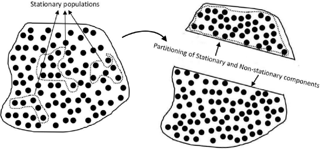
Figure 2.4. Partitions into stationary and non-stationary components of a randomly selected large population. All the populations within the dotted lines on the left hand side form the stationary component and others make non-stationary component of the total population as shown in the right side of the Figure. Note that partitioning is not about geographical partition.

∎

Remark 3.

Since we are calculating the proportion of sub-populations at each age of the actual population, we might come across values of these proportions calculated at two or more ages that could be identical. All the ages with identical proportions would fall within the same component of the population, i.e. stationary or non-stationary by the construction explained in the proof of the Theorem 2.

Remark 4.

The partition theorem can be extended to more than two partitions if there are multiple decrement life tables available for a randomly selected large population.

3. Conclusions

The main theorem stated and proved is the first such observation in the literature. Moreover, we have not come across in the literature where life table identity was being used to relate actual populations and applied to decide stationary and non-stationary components of a large randomly selected actual population. The partitioning procedure described in this work can be used to decide what proportion of the population is stationary and what proportion is not by considering the world population as a whole as one unit, individual countries, continents and groups of countries, etc, We can also apply this procedure to test the stationary and non-stationary status of all sub-regions of a large country.

The partition theorem stated and proved is not an improvement of any previously shown results in stationary populations. The statement of partition theorem in the article is original and the method demonstrated whether a component of a large population is stationary or non-stationary has not existed. A given large population or its sub-populations showing oscillatory behavior of transitioning from stationary to non-stationary and vice versa were earlier shown in [9].

With many countries in the world approaching or at replacement levels but often with widely varying if not unique age distributions, the partitioning theory outlined here has the potential to provide new metrics on age structure in particular and on overall population dynamics in general. Metrics to measure population stability status between two populations were proposed in [14]. Both of these can be used for both between-country comparisons as well as for projections into the future at both regional, national and global levels.

Acknowledgments: J.R. Carey (U.C. Davis) provided appreciation and encouragement when the author posed the statement of the partition theorem for populations for the first time in 2018. This inspired the author to finish the proof. S. Tuljapurkar (Stanford University) provided helpful comments on the previous draft. Two reviewers provided very helpful and constructive comments that very much helped in revising the article. I am greatly thankful to all. ASRS Rao has no funding support to disclose that is related to this project.

References

- [1] Muller H .G., Wang J - L, Carey J.R., Caswell - Chen E.P., Chen C., Papadopoulos N., Yao F. (2004) Demographic window to aging in the wild: Constructing life tables and estimating survival functions from marked individuals of unknown age. Aging Cell 3 , 125 - 131.
- [2] Carey, JR; Mï¿œller, HG; JL Wang, JL; Papadopoulos, NT; Diamantidis, A; Koulousis, NA (2012). Graphical and demographic synopsis of the captive cohort method for estimating population age structure in the wild. Experimental Gerontology 47 (10), 787-791.
- [3] Rao A.S.R.S. and Carey J.R. (2015). Carey’s Equality and a theorem on Stationary Population, Journal of Mathematical Biology, 71: 583-594.
- [4] Brouard, N. 1986. Structure et dynamique des populations La puramide des annees a vivre, aspects nationaux et examples regionaux.4: 157-168
- [5] Carey, J.R., Silverman, S., Rao, A.S.R.S. (2018). The life table population identity: Discovery, formulations, proofs, extensions and applications, pp: 155-185, Handbook of Statistics: Integrated Population Biology and Modelling Part A, volume 39 (Eds: Arni S.R. Srinivasa Rao and C.R. Rao), Elsevier.
- [6] Wachter, K.W. (2014). Essential Demographic Methods, Harvard University Press (1/e).
- [7] Misra, B.D. (1998) An Introduction to the Study of Population, by South Asian Publishers, New Delhi, 1995.
- [8] Preston S, Heuveline P, Guillot M (2000). Demography: Measuring and Modeling Population Processes 1st Edition Wiley-Blackwell.
- [9] Rao A.S.R.S. and Carey J.R. (2019). On three properties of stationary populations and knotting with non-stationary populations, Bulletin of Mathematical Biology, 81, 10: 4233-4250 (10.1007/s11538-019-00652-7)
- [10] Kim, Y. J. and Aron, J. L. (1989). On the equality of average age and average expectation of remaining life in a stationary population. SIAM Review 31(1): 110–113.
- [11] Cox, D. R. (1962). Renewal Theory. London: Methuen and Co.
- [12] Lotka A. J. (1925). Elements of Physical Biology, Baltimore, Williams and Wilkins Company.
- [13] Lotka, A.J. (1939). On an integral equation in population analysis. Annals of Mathematical Statistics, 10:144–161.
- [14] Rao, A.S.R.S (2014). Population Stability and Momentum, Notices of the American Mathematical Society, 62, 9: 1062-1065.