A Novel Algebraic Geometry Compiling Framework for Adiabatic Quantum Computations

Abstract

Adiabatic Quantum Computing (AQC) is an attractive paradigm for solving hard integer polynomial optimization problems, as it is robust to environmental noise. Available hardware restricts the Hamiltonians to be of a structure that allows only pairwise interactions, an aspect that will likely remain for the foreseeable future. This requires that the original optimization problem to be first converted – from its polynomial form – to a quadratic unconstrained binary optimization (QUBO) problem, which we frame as a problem in algebraic geometry. Additionally, the hardware graph where such a QUBO-Hamiltonian needs to be embedded – assigning variables of the problem to the qubits of the physical optimizer – is not a complete graph, but rather one with limited connectivity. This “problem graph to hardware graph” embedding can also be framed as a problem of computing a Groebner basis of a certain specially constructed polynomial ideal. In this paper, we develop a systematic computational approach to prepare a given polynomial optimization problem for AQC in three steps. The first step reduces an input polynomial optimization problem into a QUBO through the computation of the Groebner basis of a toric ideal generated from the monomials of the input objective function. The second step computes feasible embeddings. The third step computes the spectral gap of the adiabatic Hamiltonian associated to a given embedding. These steps are applicable well beyond the integer polynomial optimization problem. Our paper provides the first general purpose computational procedure that can be used directly as a translator to solve polynomial integer optimization. Alternatively, it can be used as a test-bed (with small size problems) to help design efficient heuristic quantum compilers by studying various choices of reductions and embeddings in a systematic and comprehensive manner. An added benefit of our framework is in designing Ising architectures through the study of $\mathcal{Y}-$minor universal graphs.

Keywords: Polynomial Optimization, Adiabatic Quantum Computing, Ising Model, Graph Embedding, Spectral Gap, Groebner basis, Fiber Bundles, Classical Invariant Theory, Compilers.

1 Introduction

Adiabatic quantum computation (AQC) is a quantum computing paradigm that solves optimization problems of the form

$$(\mathcal{P}):\,argmin_{(y_{0},\cdots,y_{m-1})\in\mathbb{B}^{m}}\,f(y_{0},\cdots,y_{m-1}),$$ (1.1)

where $\mathbb{B}=\{0,1\}$ and $f$ is a polynomial function in $y_{0},\cdots,y_{m-1}$ with rational coefficients (we write $f\in\mathbb{Q}[y_{0},\cdots,y_{m-1}]$). In order to do so, each binary variable $y_{i}$ is mapped into a quantum spin (or a qubit), and each monomial in $f$ defines a many body interaction (or coupling) between the involved spins. The collection of these interacting spins defines a quantum system (a self-adjoint $2^{m}\times 2^{m}-$matrix) whose energy (spectrum) is exactly the range of the objective function $f$. Correspondingly, the solution of the problem $(\mathcal{P})$ sits on the ground state (the eigenvector of lowest energy) of the quantum system. AQC finds the ground state by employing the adiabatic quantum evolution that slowly evolves the ground state of some known system into the sought ground state of the problem $(\mathcal{P})$.

In reality, the picture is less ideal. Available physical realizations of AQC processors (such as D-Wave Systems processors [JAG⁺11]) are built on the Ising model, where the manufactured qubits are arranged in a three dimensional graph. For instance, Figure 1 depicts the arrangement of qubits inside the D-Wave Systems 2000Q processor. Therein, as in any Ising model, each qubit can be coupled only with neighboring qubits (2-body interactions), which restricts the function $f$ to a quadratic polynomial, and the problem $(\mathcal{P})$ to a quadratic unconstrained binary optimization (QUBO) problem. Another restrictive feature of current architectures is that their hardware graphs are rather non-complete, with limited low edge densities, which makes casting the QUBO into a self-adjoint matrix, as explained above, highly non-trivial. Theoretically, we know how to overcome both restrictions: we use additional variables for the degree restriction and minor embeddings for the non-completeness restriction. The next examples describe this concept of embedding and the difficulties in finding them in practice; we skip introducing the notion of additional variables as it is well known, and for which have dedicated a section where we relate the important problem of minimizing their number to toric ideals.

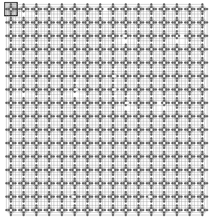
(a)

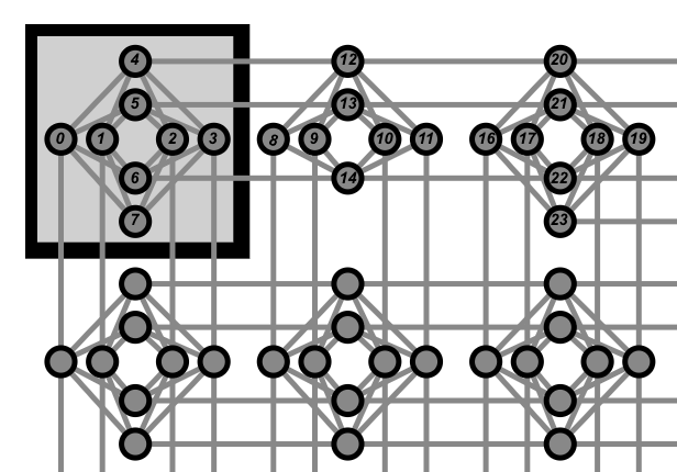
(b)

Figure 1: Cross representation of Chimera $4\times 16\times 16$, the graph of D-Wave Systems 2000Q processor (there is a second representation called column representation illustrated in the left graph of Figure 5). Qubits are arranged in $16\times 16$ blocks (or cells). Each block is a $4\times 4$ bipartite graph. Qubits have restricted connectivity along the edges where each qubits can interact/couple with at most six neighbors. The missing vertices or edges are faulty qubits or couplers.

1.1 QUBO to Hardware Embedding: Two illustrative examples

The first example serves as an illustration for the notion of QUBO to Hardware Embedding; in the second example, we demonstrate our approach and its advantage over current heuristics.

1.1.1 First example: What is a QUBO to hardware embedding?

Consider the following optimization problem that we wish to solve on the D-Wave Systems 2000Q processor:

$$(\mathcal{P}_{\star}):\,argmin_{(y_{0},\cdots,y_{m-1})\in\mathbb{B}^{m}}\quad y_{0}\sum_{i=1}^{8}c_{i}y_{i}.$$ (1.2)

(a)

Figure 2: The logical graph of the objective function in $(\mathcal{P}_{\star})$

As mentioned before, this requires assigning the problem variables $y_{0},\cdots,y_{8}$ to the physical qubits of the processor. Let us denote by $X$ the physical graph depicted in Figure 1 and by $Y$ the logical graph that represents the quadratic objective function of the problem $(\mathcal{P}_{\star})$ given in Figure 2. We can start by attempting to embed $Y$ inside $X$ by matching edges to edges; we quickly realize that this is not an option, because the degree of the vertex $y_{0}$ is 8 whilst the maximum degree in Chimera graph $X$ is 6. On the other hand, by drawing an analogy to the blowup procedure in algebraic geometry, we can blowup the singularity – here the intersection point $y_{0}$ – into a line (a chain). Figure 3 depicts three minor embeddings of $Y$, where the problem qubit $y_{0}$ is represented by a chain of physical qubits. In fact, a minor embedding can be understood as a sequence of blow ups of high degree or distant vertices. For more complicated problems, finding the right sequence of blow ups (assuming one exists) is non-trivial and is a central question of this paper. The next example discusses this point.

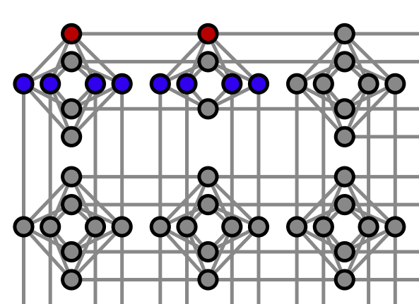
(a)

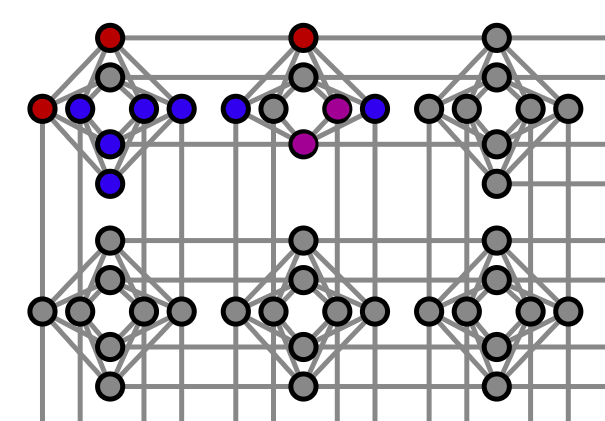
(b)

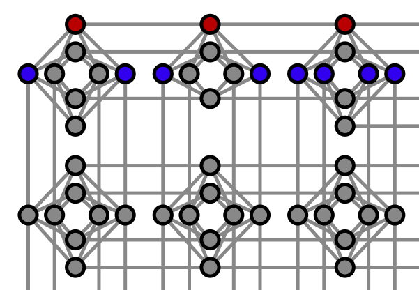
(c)

Figure 3: Three different examples of embeddings of the logical graph 2 inside Chimera. In all cases, the red chains of qubits represent the logical qubit $y_{0}$. The remaining qubits are represented with 1-chain (i.e., a physical qubit) in blue, except for the middle picture, where $y_{7}$ is represented by the purple 2-chain.

1.1.2 Second example: Demonstration of our approach

In this example, the logical graph $Y$ is given in Figure 4, and we wish, as before, to embed it inside the Chimera graph. The embedding is not hard to find by inspection: the right block of the graph $Y$ is a $4\times 4$ bipartite cell in Chimera (left graph of Figure 5), and we can embed the remaining left block (the two triangles) by collapsing (at least) one edge of a second neighboring cell. The subtlety here, however, is that the only way to embed the graph $Y$ inside a 2-blocks Chimera is by collapsing edges that are entirely contained inside one of the blocks. Any heuristic that looks for these chains otherwise will fail – it is easy to scale the example, making it very hard for current heuristics.

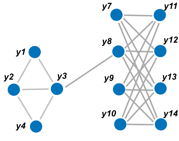
(a)

Figure 4: To embed the depicted problem graph inside Chimera $2\times 2$ (left graph of Figure 5), we need to collapse edges that are entirely contained inside one of the blocks. Heuristics that looks for these chains otherwise will fail.

We can obtain this embedding as follows. First, we think of an embedding as a surjection $\pi$ from the hardware graph $X$ to the logical graph $Y$ – the triplet $(X,Y,\pi)$ forms a fiber-bundle. This surjection $\pi$ maps a chain of physical qubits (a fiber) into at most one logical qubit. Or, if we write

$$\pi(x_{i})=\sum_{y_{j}\in{\bf Vertices}(Y)}\alpha_{ij}y_{j}$$ (1.3)

for each $x_{i}\in{\bf Vertices}(X)$, then at most one of the binary numbers $\alpha_{ij}$ is 1 for each $x_{i}$ (if the qubits $x_{i}$ is not used then we set $\pi(x_{i})=0$). So, the condition that chains should not intersect (that is, $\pi$ is a well defined map) translates into a set of algebraic equations on the parameters $\alpha_{ij}$. Similarly, all the requirements that an embedding needs to satisfy (which we will review in Subsection 4.2.1) can be formulated as a set of algebraic equations on the binary parameters $\alpha_{ij}$ (presented in Subsection 4.2.2). Therefore, the set of all embeddings (up to any desired size) is given by the set of zeros (algebraic variety) of this system. When this variety is empty, the logical graph $Y$ is not embeddable inside $X$.

In our example of Figure 4, the variety is not empty and it suffices to solve its defining system to obtain the sought embedding of the graph $Y$. However, we can do much better that this by employing invariant theory to compress the different algebraic expressions – many of the solutions are redundant (identical up to symmetries in ${\bf Aut}(X)$), which affects the efficiency of the method for large graphs. Indeed, we can get rid of this redundancy by folding the hardware graph $X$ along its symmetry axis as in Figure 5 – this folding operation is made precise and systematic in 4.2.5, where we re-express its quadratic form in terms of the invariants of the symmetry. The quadratic form of the new graph depicted in Figure 5 is

$$K_{1}K_{3}+K_{1}K_{4}+K_{2}K_{3}+K_{2}K_{4}+K_{4}K_{5}+K_{3}K_{6}+K_{8}K_{5}++K_{8}K_{6}+K_{7}K_{5}+K_{7}K_{6}.$$ (1.4)

The nodes $K_{i}$ are the invariants of the symmetry (see also the caption of Figure 5)

$$K_{1} = x_{1}+x_{2},\quad\,K_{2}=x_{3}+x_{4},\quad\,\,\,K_{3}=x_{7}+x_{8},\quad K_{4}=x_{5}+x_{6},$$ (1.5)

$$K_{5} = x_{9}+x_{10},\quad K_{6}=x_{11}+x_{12},\quad K_{7}=x_{15}+x_{16},\quad K_{8}=x_{13}+x_{14}.$$ (1.6)

The map $\pi$ now takes the form

$$\pi(K_{i})=\sum_{y_{j}\in{\bf Vertices}(Y)}\alpha_{ij}y_{j},$$ (1.7)

where the goal is to embed the problem graph of Figure 4 inside this folded Chimera. We generate the system of equations on the parameters $\alpha_{ij}$ with this new target graph and solve. We obtain the solution

$$\left\{\begin{array}[]{lll}K_{1}&=&y_{1}+y_{2},\\ K_{2}&=&K_{3}=y_{4},\\ K_{4}&=&y_{1}+y_{3},\\ K_{5}&=&y_{7}+y_{8},\\ K_{6}&=&y_{9}+y_{10},\\ K_{7}&=&y_{13}+y_{14},\\ K_{8}&=&y_{11}+y_{12}.\end{array}\right.$$ (1.15)

The first equation says that the formal sum $x_{1}+x_{2}$ maps to the formal sum $y_{1}+y_{2}$. Any choice of assigning values to $x_{1}$ and $x_{2}$ is equally valid – they were redundant before the use of invariants. The remaining equations are treated similarly. The second equation says that the nodes $K_{2}=x_{3}+x_{4}$ and $K_{3}=x_{7}+x_{8}$ collapse into the qubits $y_{4}$ hence, for instance, the edge $(x_{3},x_{7})$ collapses into $y_{4}$. Collapsing any of the edges $(x_{3},x_{8})$, $(x_{4},x_{7})$ and $(x_{4},x_{8})$ is also valid but redundant.

(a)

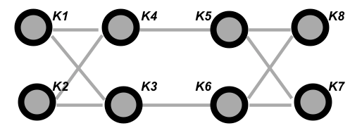
(b)

Figure 5: The left graph is (the column representation of) Chimera $2\times 2$. The permutation that exchanges the chain $[x_{1},x_{5},x_{9},x_{13}]$ with $[x_{2},x_{6},x_{10},x_{14}]$ and the chain $[x_{3},x_{7},x_{11},x_{15}]$ with $[x_{4},x_{8},x_{12},x_{16}]$, is a symmetry. The right graph is obtained by re-expressing the quadratic form of the left graph in terms of the invariants of this symmetry. Embedding the problem graph in Figure 4 inside this folded version of Chimera leads to more efficient calculations.

1.1.3 More intricacies of finding embeddings in the context of AQC

The two examples above illustrate how difficult is the problem of embedding from the algorithmic point of view. What makes this problem even more difficult is the fact that not all minor embeddings are equally useful for AQC. First, the number of physical qubits used is important (recall that the dimension of the Hilbert space is exponential in the number of qubits). Second, the size of the chains – the number of replications of an individual problem qubit that need to be linked together to form a chain – as well as their couplings has significant implications on the effectiveness of the embedding (See Figure 6). Third, as we show in this paper, the theoretical computational speedup in AQC itself depends on the choice of the minor embedding.

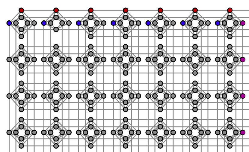
(a)

Figure 6: The depicted minor embedding (for the problem $(\mathcal{P})_{*}$) has two long chains that don’t persist through the adiabatic evolution (in D-Wave). In this case, the quantum processor fails to return an answer.

1.2 Goals of the paper

Suppose we are given a polynomial binary optimization problem

$$(\mathcal{P}):\,argmin_{(y_{0},\cdots,y_{m-1})\in\mathbb{B}^{m}}\,f(y_{0},\cdots,y_{m-1}).$$ (1.16)

In this paper, using a novel algebraic geometry perspective on AQC, we make three contributions:

• An end-to-end systematic procedure for solving optimization problems $(\mathcal{P})$, using Ising AQC processors. This translator (or compiler) can be programmed classically starting from the problem model and ending up with an input into the quantum computer. One can view this as the first fully systematic compiler for AQC.

• Computing the spectral gap of the adiabatic Hamiltonian as an algebraic function of the points of the embedding variety.

• A systematic procedure for the design of near term Ising architectures. This design problem is referred to as the $\mathcal{Y}-$minor universal problem in the literature [Cho11]. The task is to design architectures that obey the physical engineering constraints (low connectivity of the manufactured qubits) and still are able to tackle interesting, hard problems.

We recognize that the (worst-case) computational complexity of our procedure is not polynomial. Indeed, at this time, we are interested primarily in developing a robust theoretical framework that can form the basis of a computational procedure that can be programmed into software, and laying out the various issues that arise as we move from optimizing polynomials on lattices to creating embeddable Hamiltonians on physically realizable architectures. This allows us to study small problem instances in a systematic and comprehensive manner on actual physical devices. Thus, our framework can serve as a sandbox to test various heuristics to help design an efficient and scalable (that may have a provable worst-case polynomial time performance) quantum compiler. Similarly, through the study of the $\mathcal{Y}-$minor universal problem, we can help design good, physically realizable hardware.

• Flowchart of the Translator:

• The user inputs the optimization problem $(\mathcal{P})$.

• Reduction to a quadratic form: (Details in Section 4.1)

  • Generation of the toric ideal $\mathcal{J}_{A}$ from the monomials of the objective function of $(\mathcal{P})$.

  • Computation of a reduced Groebner basis for $\mathcal{J}_{A}$; return the quadratic function ${\mathcal{E}\in\mathbb{Q}[y]}$.

• Embedding inside the AQC processor graph: (Details in Section 4.2)

  • Generation of the ideal $\mathcal{I}$ that gives the minor embeddings $\pi$.

  • Computation of a reduced Groebner basis $\mathcal{B}$ of the ideal $\mathcal{I}$.

  • If $1\in\mathcal{B}$. Go back to 2 and choose a different quadratic function.

  • Comparison of the different embeddings with respect to their effect on the spectral gap. (Details in Section 4.3)

• Solution using a selected embedding on the AQC processor.

• User gets the answer.

1.3 Outline of the Paper

The paper is structured as follows. Section 2 briefly summarizes AQC on Ising spin glass architectures. Section 3 briefly reviews Groebner bases, toric ideals, and related useful results. Section 4.1 uses toric ideals to provide an algorithm for the reduction step, resulting in a QUBO. Section 4.2 details the calculation of minor-embedding using Groebner bases. We show that the set of all embeddings is an algebraic variety. The automorphisms of the hardware graph, specifically their invariants, are used to help with the computation. We also show how the number of minor-embeddings is determined using staircase diagrams. Section 4.3 provides a method to compute the spectral gap as an algebraic function of the points of the embedding variety. In section 5, we solve the problem of $\mathcal{Y}$-minor embedding universal [Cho08] using Groebner bases. We conclude in Section 6.

Notations

All graphs considered here are simple and undirected. The following notation is used in the remainder of the paper:

• ${\bf Vertices}(X)$ and ${\bf Edges}(X)$ are the vertex and edge sets of the graph $X$.

• $n=card({\bf Vertices}(X))$ is the size of the hardware graph $X$.

• $m=card({\bf Vertices}(Y))$ is the size of the problem graph $Y$.

• ${\bf Vertices}(X)=\{x_{0},\cdots,x_{n-1}\}$ and $x=(x_{0},\cdots,x_{n-1})$.

• ${\bf Vertices}(Y)=\{y_{0},\cdots,y_{m-1}\}$ and $y=(y_{0},\cdots,y_{m-1})$.

• $\mathbb{Q}[x_{0},\cdots,x_{n-1}]$ the ring of polynomials in $x_{0},\cdots,x_{n-1}$ with rational coefficients.

• $Q_{X}(x):=\sum_{x_{i_{1}}x_{i_{2}}\in{\bf Edges}(X)}x_{i_{1}}x_{i_{2}}\in\mathbb{Q}[x_{0},\cdots,x_{n-1}]$ is the quadratic form of the graph $X$.

• $Q_{Y}(y):=\sum_{y_{j_{1}}y_{j_{2}}\in{\bf Edges}(Y)}y_{j_{1}}y_{j_{2}}\in\mathbb{Q}[y_{0},\cdots,y_{m-1}]$ is the quadratic form of the graph $Y$.

• $\alpha=(\alpha_{ij},\,i=0..n-1,j=0..m-1)$.

• $\beta=(\beta_{0},\cdots,\beta_{n-1})$.

• $u=(u_{0},\cdots,u_{n-1})$ and $x^{u}=x_{0}^{u_{0}}\cdots x_{n-1}^{u_{n-1}}$.

2 The Physics: AQC on Ising Spin Glass Architectures

The primary purpose of Adiabatic quantum computation (AQC) [FGG⁺01, KN98] is to solve the problem of computing ground states of high dimensional Hamiltonians (self-adjoint operators acting on large Hilbert spaces, usually ${{\mathbb{C}^{2}}^{\otimes n}:={\mathbb{C}^{2}}\otimes\cdots\otimes{\mathbb{C}^{2}}}$). It is a straightforward application of the adiabatic theorem [BF28, Kat50, AE99] to time dependent Hamiltonians of the form

$$H(t)=(1-t/T)H_{initial}+tH_{(\mathcal{P})}.$$ (2.1)

This theorem states that the quantum system, initialized at the known ground state of the initial Hamiltonian $H_{initial}$, will remain at the ground state of $H(t)$ for all time $t\leq T$ with probability inversely proportional to the square of the energy difference with the rest of the spectrum. A simple series expansion of the wave function in the slow regime (see for instance [KN98]) shows that the total time $T$ spent to adiabatically attain the sought ground state is

$$T\sim O\left(\frac{1}{min_{0\leq t\leq T}\Delta(t)}\right)$$ (2.2)

where $\Delta(t)$ is the gap between the two smallest eigenvalues (spectral gap) of $H(t)$. A measurement of the final state will yield a solution of the problem. A notable fact about AQC is that it enjoys proved robustness against environment noise [CFP01, JFS06] (as long as the temperature of the environment is not too high), making AQC a reasonable choice for near term quantum computing,

As mentioned before, only the restricted class of Ising spin glass Hamiltonians (Ising Hamiltonians for short) is currently physically realized. The quantum system is constituted of a set of spins that can point to two directions and are arranged in a graph $X$ where only local 2-body interactions, along the edges of $X$, are allowed (See Figure 1). More formally, Ising Hamiltonians are of the form

$$H_{(\mathcal{P})}=\sum_{i\in{\bf Vertices}(X)}h_{i}\sigma_{i}^{3}+\sum_{ij\in{\bf Edges}(X)}J_{ij}\sigma^{3}_{i}\sigma^{3}_{j},$$ (2.3)

with $\sigma_{i}^{3}=I\otimes\cdots\otimes\sigma^{3}\otimes\cdots\otimes I$ and $\sigma^{3}_{i}\sigma^{3}_{j}=I\otimes\cdots\otimes\sigma^{3}\otimes\cdots\otimes\sigma^{3}\otimes\cdots\otimes I$. Here, $\sigma^{3}$ is the Pauli operator

$$\sigma^{3}=\begin{bmatrix}1&0\\ 0&-1\end{bmatrix}$$ (2.4)

and $I$ is the $2\times 2$ identity matrix. The coefficients $h_{i}$ are the biases and the coefficients $J_{ij}$, called couplings, determine the strength of the interactions between the two spins $\sigma^{3}_{i}$ and $\sigma^{3}_{j}$. When the coupling $J_{ij}$ is negative, in which case we say $J_{ij}$ is a ferromagnetic coupling, the two spins tend to point to the same direction. Inversely, when $J_{ij}$ is positive, anti-ferromagnetic coupling, the two spins point to opposite directions. With different coupling strengths and signs, the aggregated interaction is, in general, complicated, and computing the ground state of $H_{(\mathcal{P})}$ is NP [Bar82, Luc14]. Note that, with the restriction to Ising architecture, AQC is no longer universal [AvDK⁺04, MLM07].

The Hamiltonian $H_{(\mathcal{P})}$ is intentionally made diagonal in the computational basis; that is, vectors of the computational basis are eigenstates of $H_{(\mathcal{P})}$. Consequently, calculating the scalar products $\langle y_{1}\cdots y_{m}|H_{(\mathcal{P})}|y_{1}\cdots y_{m}\rangle$ gives the energy function of $H_{(\mathcal{P})}$:

$$\mathcal{E}_{(\mathcal{P})}(s_{1},\cdots,s_{n})=\sum_{i\in{\bf Vertices}(X)}h_{i}s_{i}+\sum_{ij\in{\bf Edges}(X)}J_{ij}s_{i_{1}}s_{i_{2}},$$ (2.5)

where $s_{i}\in\{-1,1\}$ or by taking $x_{i}=(s_{i}+1)/2$ (consistently with 01-notation in binary optimization):

$$\mathcal{E}_{(\mathcal{P})}(x_{1},\cdots,x_{n})=\sum_{i\in{\bf Vertices}(X)}h_{i}x_{i}+\sum_{ij\in{\bf Edges}(X)}J_{ij}x_{i_{1}}x_{i_{2}},$$ (2.6)

where we have used the same notations $h_{i}$ and $J_{ij}$ for the new adjusted coefficients. The energy function measures the violations, by the given spin configuration, of the ferromagnetic and anti-ferromagnetic couplings. The ground state of the Hamiltonian $H_{(\mathcal{P})}$ coincides with the spin configuration with the minimum amount of violations, which is also the global minimum of the energy function.

Optimization problems	Adiabatic quantum computations
Polynomial binary optimization	Many-body (many-spin) Hamiltonian
Quadratic binary optimization	Ising Hamiltonian
Objective function	Energy function
Binary variables $y_{i}$	Qubit $|y_{i}\rangle$ i.e., state of the $i$th spin $\sigma^{3}$
Monomials $J_{ij}y_{i}y_{j}$	Coupled spins with Coupling strengths $J_{ij}$
Global minima	Ground state (possibly degenerate)
Local minima	States (spectrum) of the Hamiltonian
Search space $\{0,1\}^{n}$	Hilbert space ${\mathbb{C}^{2}}^{\otimes n}$

Table 1: Correspondence between optimization problems and adiabatic quantum computations.

There are several proposals for the initial Ising Hamiltonian $H_{initial}$, all with the property that cooling to their ground states is easy. Our exposition doesn’t depend on the choice of the Hamiltonian $H_{initial}$.

3 The Mathematics: Groebner Basis and Toric Ideals

The intertwining between algebraic geometry and optimization is a fertile research area. The collective work of B. Sturmfels and collaborators [Stu96, PS01] is of particular interest. The application of algebraic geometry to integer programming can be found in [CT91, TTN95, ST97, BPT00]. Sampling from conditional distributions is suggested in [DS98]. Application to prime factoring in conjunction with AQC is explored in [DA17].

Let $\mathcal{S}$ be a set of polynomials $f\in\mathbb{Q}[x_{0},\ldots,x_{n-1}]$. Let $\mathcal{V}(S)$ denotes the affine algebraic variety defined by the polynomials $f\in S$, that is, the set of common zeros of the equations $f=0,\,f\in\mathcal{S}$. The system $\mathcal{S}$ generates an ideal $\mathcal{I}$ by taking all linear combinations over $\mathbb{Q}[x_{0},\ldots,x_{n-1}]$ of all polynomials in $\mathcal{S}$; we have $\mathcal{V}(\mathcal{S})=\mathcal{V}(\mathcal{I}).$ The ideal $\mathcal{I}$ reveals the hidden polynomials that are the consequence of the generating polynomials in $\mathcal{S}$. For instance, if one of the hidden polynomials is the constant polynomial 1 (i.e., $1\in\mathcal{I}$), then the system $\mathcal{S}$ is inconsistent (because $1\neq 0$).

Strictly speaking, the set of all hidden polynomials is given by the so-called radical ideal $\sqrt{\mathcal{I}}$, which is defined by $\sqrt{\mathcal{I}}=\{g\in\mathbb{Q}[x_{0},\ldots,x_{n-1}]|\,\exists r\in\mathbb{N}:\,g^{r}\in\mathcal{I}\}$. In practice, the ideal $\sqrt{\mathcal{I}}$ is infinite, so we represent such an ideal using a Groebner basis $\mathcal{B}$, which one might take to be a triangularization of the ideal $\sqrt{\mathcal{I}}$. In fact, the computation of Groebner bases generalizes Gaussian elimination in linear systems. We also have $\mathcal{V}(\mathcal{S})=\mathcal{V}(\mathcal{I})=\mathcal{V}(\sqrt{\mathcal{I}})=\mathcal{V}(\mathcal{B})$ and (Hilbert’s Nullstellensatz theorem:) $\mathcal{I}(\mathcal{V}(\mathcal{I}))=\sqrt{\mathcal{I}}$.

Term orders. A term order on $\mathbb{Q}[x_{0},\ldots,x_{n-1}]$ is a total order $\prec$ on the set of all monomials $x^{a}=x_{1}^{a_{1}}\ldots x_{n}^{a_{n}}$, which has the following properties:

• if $x^{a}\prec x^{b}$, then $x^{a+c}\prec x^{b+c}$ for all positive integers $a,b$, and $c$;

• $1\prec x^{a}$ for all strictly positive integers $a$.

An example of this is the pure lexicographic order plex $x_{0}\succ x_{1}\succ\cdots$. Monomials are compared first by their degree in $x_{0}$, with ties broken by degree in $x_{1}$, etc. This order is usually used in eliminating variables. Another example, is the graded reverse lexicographic order tdeg. Monomials are compared first by their total degree, with ties broken by reverse lexicographic order. This order typically provides faster Groebner basis computations.

Groebner bases. Given a term order $\prec$ on $\mathbb{Q}[x_{0},\ldots,x_{n-1}]$, then by the leading term (initial term) LT of $f$ we mean the largest monomial in $f$ with respect to $\prec$. A reduced Groebner basis to the ideal $\mathcal{I}$ with respect to the ordering $\prec$ is a subset $\mathcal{B}$ of $\mathcal{I}$ such that:

• the initial terms of elements of $\mathcal{B}$ generate the ideal ${\sf LT}(\mathcal{I})$ of all initial terms of $\mathcal{I}$;

• for each $g\in\mathcal{B}$, the coefficient of the initial term of $g$ is 1;

• the set ${\sf LT}(g)$ minimally generates ${\sf LT}(\mathcal{I})$; and

• no trailing term of any $g\in\mathcal{B}$ lies in ${\sf LT}(\mathcal{I})$.

Currently, Groebner bases are computed using sophisticated versions of the original Buchberger algorithm, for example, the F4 and F5 algorithms by J. C. Faugère [Fau99].

Theorem 1

Let $\mathcal{I}\subset\mathbb{Q}[x_{0},\ldots,x_{n-1}]$ be an ideal and let $\mathcal{B}$ be a reduced Groebnber basis of $\mathcal{I}$ with respect to the lex order $x_{0}\succ\ldots\succ x_{n-1}$. Then, for every $0\leq l\leq n-1$, the set

$$\mathcal{B}\cap\mathbb{Q}[x_{l},\ldots,x_{n-1}]$$ (3.1)

is a reduced Groebner basis of the ideal $\mathcal{I}\cap Q[x_{l},\ldots,x_{n-1}]$.

We shall use this elimination theorem repeatedly in this paper. It is used to obtain the complete set of conditions on the variables $x_{l},\ldots,x_{n-1}$ such that the ideal $\mathcal{I}$ is not empty. For instance, if the ideal represents a system of algebraic equations and these equations are (algebraically) dependent on certain parameters, then the intersection (3.1) gives all necessary and sufficient conditions for the existence of solutions.

Normal forms. A normal form is the remainder of Euclidean divisions in the ring of polynomials $k[x_{0},\ldots,x_{n-1}]$. Precisely, let $\mathcal{B}$ be a reduced Groebner basis for an ideal $\mathcal{I}\subset k[x_{0},\ldots,x_{n-1}]$. The normal form of a polynomial $f\in\mathbb{Q}[x_{0},\ldots,x_{n-1}]$, with respect to $\mathcal{B}$, is the unique polynomial ${{\sf NF}_{\mathcal{B}}(f)\in\mathbb{Q}[x_{0},\ldots,x_{n-1}]}$ that satisfies the following properties:

• No term of ${\sf NF}_{\mathcal{B}}(f)$ is divisible by an ${\sf LT}(p),\,p\in\mathcal{B}$

• There is $g\in\mathcal{I}$ such that $f=g+{\sf NF}_{\mathcal{B}}(f)$. Additionally, ${\sf NF}_{\mathcal{B}}(f)$ is the remainder of division of $f$ by $\mathcal{B}$ no matter how elements of $\mathcal{B}$ are listed when performing the Euclidean division.

The remainder ${\sf NF}_{\mathcal{B}}(f)$ is the canonical representative for the equivalence class of $f$ modulo $\mathcal{I}$. If one knows that $1\notin\mathcal{I}$, the generalized division algorithm  ([CLO07], Chapter 2) can be applied directly using $\mathcal{I}$ and the given monomial order, without computing Groebner bases. However, in this case, the result is not always equal to the canonical remainder that $\mathcal{B}$ gives.

Toric ideals. These are ideals generated by differences of monomials. Their Groebner bases enjoy a clear structure given by kernels of integer matrices. Specifically, let $A=(a_{1},\cdots,a_{n})$ be any integer $m\times n$-matrix ($A$ is called configuration matrix). Each column ${{\bf a}}_{i}=(a_{1i},\cdots,a_{ni})^{T}$ is identified with a Laurent monomial $y^{{{\bf a}}_{i}}=y_{1}^{a_{1i}}\cdots y_{m}^{a_{ni}}$. The toric ideal $\mathcal{J}_{A}$ associated with the configuration $A$ is the kernel of the algebra homomorphism

$$\mathbb{Q}[x]\rightarrow\mathbb{Q}[y]$$ (3.2)

$$x_{i}\mapsto y^{{{\bf a}}_{i}}.$$ (3.3)

We have:

Proposition 1

The toric ideal $\mathcal{J}_{A}$ is generated by the binomials $x^{{{\bf u}}_{+}}-x^{{{\bf u}}_{-}},$ where the vector ${\bf u}={{\bf u}}_{+}-{{\bf u}}_{-}\in{\mathbb{Z}^{+}}^{n}\oplus{\mathbb{Z}^{+}}^{n}$ runs over all integer vectors in $\mathrm{Ker}_{\mathbb{Z}}A$, the kernel of the matrix $A$.

Assuming $A\subset\mathbb{N}^{n}$, a conceptually easy method for computing generators of $\mathcal{J}_{A}$ is to use the elimination theorem as follows (more efficient algorithms, based on Proposition 1, are described in [Stu96]): Consider the polynomial ring $\mathbb{Q}[x,y]$ and define the ideal $\mathcal{K}_{A}$ of $\mathbb{Q}[x,y]$ by

$$\mathcal{K}_{A}=<x_{1}-y^{{{\bf a}}_{2}},\,x_{2}-y^{{{\bf a}}_{2}},\,\cdots,x_{n}-y^{{{\bf a}}_{n}}>.$$ (3.4)

The toric ideal $\mathcal{J}_{A}\subset\mathbb{Q}[x]$ of $A$ is equal to the intersection of the ideal $\mathcal{K}_{A}\subset\mathbb{Q}[x,y]$ and the ring $\mathbb{Q}[x]$; that is $\mathcal{J}_{A}=\mathcal{K}_{A}\cap\mathbb{Q}[x].$ If we consider the plex order on $\mathbb{Q}[x,y]$ induced by the ordering $y_{i}\succ x_{i}$ and compute the reduced Groebner basis $\mathcal{B}$ of $\mathcal{K}_{A}$ with respect to this plex, then the intersection $\mathcal{B}\cap\mathbb{Q}[x]$ is the reduced Groebner basis of $\mathcal{J}_{A}$. In particular, $\mathcal{B}\cap\mathbb{Q}[x]$ is a system of generators of $\mathcal{J}_{A}$.

4 The Mathematics that Enables Physics to Optimize Polynomial Programs

In the context of AQC, compiling the binary optimization problem

$$(\mathcal{P}):\,argmin_{(y_{0},\cdots,y_{m-1})\in\mathbb{B}^{m}}\,f(y_{0},\cdots,y_{m-1})$$ (4.1)

into the hardware graph consists of two steps: 1) reducing the objective function of $(\mathcal{P})$ into quadratic function and 2) embedding this function into the hardware graph. In this long section, we algorithmize these two steps using algebraic geometry. We start with the first:

4.1 Reductions to quadratic optimization and toric ideals

Consider the step of reducing the polynomial optimization $(\mathcal{P})$ to a quadratic optimization. We have explained in the introduction that this is a key step in the process of mapping the problem $(\mathcal{P})$ into a valid input for Ising based AQC processors. First of all, if we are not worried about the number of the extra variables, then this reduction can be done in a fairly easy, quick way. The idea is to replace each pair $y_{i}y_{j}$ with a new additional variable $x_{k}$ and add the following expression

$$M\times\bigg{(}a_{{1}}\left(x_{{k}}y_{{i}}-x_{{k}}\right)+a_{{2}}\left(x_{{k}}y_{{j}}-x_{{k}}\right)+a_{{3}}\left(y_{{i}}y_{{j}}-x_{{k}}\right)\bigg{)}$$ (4.2)

as a penalty term (with a large positive coefficient $M$ ) to the new function, in order to enforce the equality $x_{k}=y_{i}y_{j}$. The real numbers $a_{1},a_{2},$ and $a_{3}$ are subject only to $a_{{1}}<-a_{{3}},\,a_{{2}}<-a_{{3}},$ and $a_{{3}}>0$ (accommodating the dynamical ranges of the hardware parameters - See [DA17]).

The connection to toric ideals appears when we try to minimize the number of the additional variables (this is certainly desirable, because additional variables are wasted qubits). This optimization is now NP-hard – See [BH02]. Let us consider the ideal $\mathcal{K}_{A}$ given by

$$\mathcal{K}_{A} = \big{\langle}x_{1}-y_{1},\,x_{2}-y_{2},\,x_{3}-y_{3},\,\cdots,\,x_{m}-y_{m},$$

$$\quad x_{k}-y_{i_{1}}y_{i_{2}},\,\mbox{ for each pair }(y_{i_{1}},y_{i_{2}})\mbox{ contained in }f\big{\rangle},$$

where $k$ runs from 1 to $m+n^{\prime}$, where $n^{\prime}$ is the total number of such pairs (with $n^{\prime}+m\leq n$). The configuration matrix can be readily extracted from the powers of $y$ (See example below). We are interested in computing the toric ideal $\mathcal{J}_{A}=\mathcal{K}_{A}\cap\mathbb{Q}[x]$ that gives the algebraic relations between the variables $x_{i}$ (in particular, between the variables $x_{i}$ with $i>m$). In fact, the reduced Groebner basis $\mathcal{B}$ of $\mathcal{K}_{A}$ with respect to the plex order $y\succ x$ has “two parts”: the toric ideal $\mathcal{J}_{A}$ and a rewriting system that we use to obtain the minimal quadratic function.

Proposition 2

Let $\mathcal{B}$ be the reduced Groebner basis of the ideal $\mathcal{K}_{A}$ with respect to the plex order ${y\succ x}$. A minimal reduction of the polynomial function $f$ into a quadratic function can be constructed from the generators of $\mathcal{B}$ if $f$ is at most quartic and by repeatedly applying this procedure if the degree of $f$ is higher than four.

Before illustrating this Proposition on a concrete example, let us note the following remarks:

(a) A direct corollary of this Proposition is a re-affirmation that the computation of minimal reductions is NP-hard because computing the generators of $\mathcal{B}$, given by the kernel $\mathrm{Ker}_{\mathbb{Z}}A$ in Proposition 1, is NP-hard.

(b) The ideal $\mathcal{K}_{A}$ itself is a reduced Groebner basis with respect to the plex order $x\succ y$; thus, one can compute the normal form ${\sf NF}_{\mathcal{K}_{A}}(f)$ (it makes sense to do so). If $f$ is quartic, then the polynomial ${\sf NF}_{\mathcal{K}_{A}}(f)$ is quadratic. In general, repeated application of the same procedure will yield a quadratic function in polynomial time (by performing Euclidean divisions using the $O(n^{2})$ generators of $\mathcal{K}_{A}$). This quadratic function is, however, clearly not minimal. The minimal reduction is obtained by reversing the plex order (as in the proposition above).

(c) Multiple choices through different reductions of the objective function are desirable. This gives even more possibilities for minor-embeddings with potentially different behaviours of the adiabatic Hamiltonian.

Example 1

Consider the cubic polynomial

$$f(y_{{1}},y_{{2}},y_{{3}},y_{{4}},y_{{5}})=y_{{1}}y_{{2}}y_{{3}}+y_{{1}}y_{{3}}y_{{4}}+y_{{1}}y_{{3}}y_{{5}}+y_{{2}}y_{{3}}y_{{5}}+y_{{3}}y_{{4}}y_{{5}},$$ (4.4)

where our objective is to reduce $f$ into a quadratic polynomial that has the same global minima as $f$. Note that such cubic objective functions can be found in 3Sat problems. The configuration matrix is given. by

$$A=\left[\begin{array}[]{cccccccccccccc}1&0&0&0&0&1&1&1&1&0&0&0&0&0\\ \vskip 6.0pt plus 2.0pt minus 2.0pt\cr 0&1&0&0&0&1&0&0&0&1&1&0&0&0\\ \vskip 6.0pt plus 2.0pt minus 2.0pt\cr 0&0&1&0&0&0&1&0&0&1&0&1&1&0\\ \vskip 6.0pt plus 2.0pt minus 2.0pt\cr 0&0&0&1&0&0&0&1&0&0&0&1&0&1\\ \vskip 6.0pt plus 2.0pt minus 2.0pt\cr 0&0&0&0&1&0&0&0&1&0&1&0&1&1\end{array}\right]$$ (4.5)

where for instance, the sixth column represents the difference of monomials $x_{6}-y_{1}y_{2}\in\mathcal{K}_{A}$ that one gets from the first monomial of $f$. The five first columns represent the differences $x_{i}-y_{i}\in\mathcal{K}_{A}$ for $1\leq i\leq 5$. Calculating the normal form ${\sf NF}_{\mathcal{K}_{A}}(f)$ gives the reduction:

$${\sf NF}_{\mathcal{K}_{A}}(f)=y_{{1}}x_{{10}}+y_{{1}}x_{{12}}+y_{{1}}x_{{13}}+y_{{2}}x_{{13}}+y_{{3}}x_{{14}},$$ (4.6)

where the extra variables are given by $x_{{10}}=y_{{2}}y_{{3}},\,x_{{12}}=y_{{3}}y_{{4}},\,x_{{13}}=y_{{3}}y_{{5}},\,x_{{14}}=y_{{4}}y_{{5}}$. Clearly, ${\sf NF}_{\mathcal{K}_{A}}(f)$ is not minimal, and the number of the extra variables can be reduced. So we compute a Groebner basis for the same ideal $\mathcal{K}_{A}$, now, with respect to the plex order $y\succ x$. This basis contains the following polynomials:

$$y_{{3}}x_{{14}}-y_{{4}}x_{{13}},\,y_{{1}}x_{{13}}-y_{{5}}x_{{7}},\,y_{{1}}x_{{12}}-y_{{4}}x_{{7}},\,y_{{1}}x_{{10}}-y_{{2}}x_{{7}},$$ (4.7)

which we think of as a rewriting system, that is a set of replacement rules where, for instance, $y_{{3}}x_{{14}}$ is replaced by $y_{{4}}x_{{13}}$. We can then re-expresses the polynomial (4.6) into the minimal reduction that has only two extra variables, $x_{7}$ and $x_{13}$.

4.2 Algebraic geometry for graph embeddings

This subsection discusses the second step in the process of compiling an optimization problem $(\mathcal{P})$ on an Ising AQC processor (the first being the reduction to QUBOs described in subsection 4.1) . The subsection is a relatively long section, so we give here a short summary. We begin by recalling the definition of a minor embedding which is a mapping

$$\phi:Y\rightarrow X$$

from the space of logical qubits to the space of physical qubits. The logical qubit $y$ is mapped to a chain (or generally, a connected subtree) of $X$. We then flip this definition and introduce an equivalent formulation: the embedding $\phi$ gives rise to a fiber-bundle

$$\pi:X\rightarrow,Y$$

where the fibers of the surjection $\pi$ are the chains (connected subtrees) of $X$ given by $\phi$:

$$\pi^{-1}(y)=\phi(y).$$

With this new definition, we express the surjection $\pi$ equationally: each physical vertex of $X$ is a formal linear combination of the vertices of $Y$, and the different constraints on $\phi$ translate into algebraic conditions on the coefficients of these linear combinations. In other words, the set of the fiber bundles $\pi$ (equivalently the set of embeddings $\phi$) is an algebraic variety (of finite cardinality). The theory of Groebner bases can be therefore applied to investigate this variety. In particular, we systematically answer the following questions:

• Existence (or non existence) of embeddings $\phi:Y\rightarrow X$.

• Calculating all embeddings $\phi:Y\rightarrow X$ in a compact form given by a Groebner basis.

• Counting all embeddings $\phi:Y\rightarrow X$ without solving any equations.

We do so for any fixed size of the chains. In the last part of the section, we discuss that many of the embeddings are redundant; that is they are of the form $\pi\circ\sigma$ with $\sigma$ a symmetry of the hardware graph $X$. This undesired redundancy (which affects the efficiency of the computations) can be removed by expressing our problem of finding $\pi$ in terms of the invariants of the symmetry $\sigma$ bringing a nice connection with the theory of invariants. Many calculations are done only once (as long as the hardware doesn’t change), and we illustrate the computational benefit with a simple concrete example.

4.2.1 Embeddings

In subsection 4.1, we have explained how the optimization problem $(\mathcal{P})$ can be reduced into the quadratic optimization problem

$$argmin_{(y_{0},\cdots,y_{m-1})\in\mathbb{B}^{m}}\,\sum_{(y_{i_{1}},y_{i_{2}})\in{\bf Edges}(Y)}J_{i_{1}i_{2}}y_{i_{1}}y_{i_{2}}+\sum_{j=0}^{m-1}h_{j}y_{j}.$$ (4.8)

This reduction is only the first step in the process of compiling the initial $(\mathcal{P})$ on Ising based AQC processors. The next step is to map or to embed the associated logical graph $Y$ into the processor graph $X$. We have mentioned that this is essentially a sequence of blowups of vertices of $Y$ of high degrees. We now define the notion of embedding more precisely

Definition 1

Let $X$ be a fixed hardware graph. A minor-embedding of the graph $Y$ is a map

$$\phi:{\bf Vertices}(Y)\rightarrow\mbox{{\bf connectedSubtrees}}(X)$$ (4.9)

that satisfies the following condition for each: $(y_{1},y_{2})\in{\bf Edges}(Y)$, there exists at least one edge in ${\bf Edges}(X)$ connecting the two subtrees $\phi(y_{1})$ and $\phi(y_{2})$.

The condition that each vertex model $\phi(y)$ is a connected subtree of $X$ can be relaxed into $\phi(y)$ is a connected subgraph i.e., $\phi(y)\in\mbox{{\bf connectedSubgraphs}}(X)$. Both cases are considered here.

In the literature there is another, but equivalent definition of minor embedding in terms of deleting and collapsing the edges of $X$. This follows from the fact that, given a minor-embedding $\phi$, the graph $Y$ can be recovered from $X$ by collapsing each set $\phi(y)$ (into the vertex $y$) and ignoring (deleting) all vertices of $X$ that are not part of any of the subtrees $\phi(y)$.

Obviously, direct graph embeddings (i.e., inclusion graph homomorphisms $Y\hookrightarrow X$) are trivial examples of minor embeddings with $\phi(y)$ reducing to a vertex in ${\bf Vertices}(X)$ for all $y\in{\bf Vertices}(Y)$. Therefore, and for the sake of a simple and clean terminology, we shall use the term embedding instead of minor-embedding throughout the remainder of the paper.

Suppose $\phi$ is an embedding of the graph $Y$ inside the graph $X$ as in Definition 1. The subgraph of $X$ given by

$$\phi(Y):=\cup_{y\in{\bf Vertices}(Y)}\phi(y)$$ (4.10)

is called a $Y$ minor (in graph minor theory). In the context of quantum computations, it represents what the quantum processor sees, because it doesn’t distinguish between normal qubits and chained qubits. For instance, in examples of Figure 3, $\phi(Y)$ is the induced subgraph defined by the colored vertices. In other words, the graph $\phi(Y)$ doesn’t keep track of where each logical qubit is mapped to. This information is stored in the hash map:

$$id\times\phi:{\bf Vertices}(Y)\times{\bf Vertices}(Y)\rightarrow{\bf Vertices}(Y)\times\mbox{{\bf Subtrees}}(X),$$ (4.11)

which is used to unembed the solution returned by the quantum processor. The numerical value of the logical qubit $y$ is the sum mod 2 of its replicates values (a strong ferromagnetic coefficient is used to enforce these replicated values to be equal, i.e., acting like a single qubit). Let us finish this review by mentioning the existence of heuristics for finding embeddings – see for instance [CMR14, BKR16] and the references therein.

4.2.2 Fiber bundles

In this subsection we describe a new computational approach for finding embeddings. The key point here is that the set of embeddings is an algebraic variety, that is the set of zeros of a system of polynomial equations. This point becomes clear if we think of embeddings as mappings from the space of physical qubits to the space of logical qubits, which is the opposite direction of the commonly used definition 1. Indeed, the embedding $\phi$ defines a fiber bundle:

$$\pi:{\bf Vertices}(X)\rightarrow{\bf Vertices}(Y)\cup\{0\}$$ (4.12)

where the pre-image (fiber) at each vertex $y\in{\bf Vertices}(Y)$ is the (vertex set of the) connected subtree $\phi(y)$ of $X$ (per Definition 1). The pre-image $\pi^{-1}(0)$ is the set of all physical qubits that are not used (they all project to zero). The reason for mapping unused qubits to zero will become clear soon (when we extend the definition $\pi$ to polynomials). A direct corollary of this representation, is that the map $\pi$ has the form:

$$\pi(x_{i}) = \sum_{j}\alpha_{ij}y_{j}$$

with $$\sum_{j}\alpha_{ij}=\beta_{i},\quad\alpha_{ij_{1}}\alpha_{ij_{2}}=0,\quad\alpha_{ij}(\alpha_{ij}-1)=0,$$

where the binary number $\beta_{i}$ is equal to one if the physical qubits $x_{i}$ is used and zero otherwise. We write $domain(\pi)={\bf Vertices}(X)$ and $support(\pi)={\bf Vertices}(X^{\beta})$ with $X^{\beta}\subset X$ the subgraph (4.10) defined by $\phi$. The fiber of the map $\pi$ at $y_{j}\in{\bf Vertices}(Y)$ is given by

$$\pi^{-1}(y_{j})=\phi(y_{j})=\{x_{i}\in{\bf Vertices}(X)|\quad\alpha_{ij}=1\}.$$ (4.14)

The conditions on the parameters $\alpha_{ij}$ guarantee that fibers don’t intersect (i.e., $\pi$ is well defined map).

Example 2

Let $X$ and $Y$ be the two graphs depicted in Figure 7. An example of the map $\pi$ is defined by $\pi(x_{1})=\pi(x_{4})=y_{1}$ and $\pi(x_{2})=y_{2}$ and $\pi(x_{3})=y_{3}$.

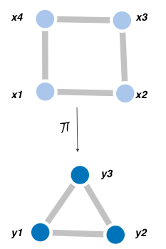
(a)

Figure 7: An example of a fiber bundle of the form (4.12).

4.2.3 Finding embeddings

Before we go deeper in the discussion, we note that the number of usable physical qubits can be constrained: we fix the maximum size of the fibers $\pi^{-1}(y_{j})$ to a certain size $k\leq\operatorname{card}({\bf Edges}(X))$. This additional size condition can be enforced using:

$$\forall j:\quad\sum_{x_{i}\in{\bf Vertices}(X)}\alpha_{ij}\leq k\quad\mbox{ or equivalently }\quad\Pi_{\kappa=1}^{k}\left(\sum_{x_{i}\in{\bf Vertices}(X)}\alpha_{ij}-\kappa\right)=0.$$ (4.15)

Additionally, we have

$$\forall j:\quad\alpha_{i_{1}j}\alpha_{i_{2}j}=0,$$ (4.16)

for all pairs $(x_{i_{1}},x_{i_{2}})$ with $d(x_{i_{1}},x_{i_{2}})>k,$ where $d(x_{i_{1}},x_{i_{2}})$ is the size of the shortest chain connecting $x_{i_{1}}$ and $x_{i_{2}}$.

The goal of the remainder of this subsection is to translate the two conditions on $\phi$, described in Definition 1, into a set of polynomial constraints on the parameters $\alpha_{ij}$ and $\beta_{i}$. For convenience, we recall the two conditions:

• Connected Fiber Condition: each fiber $\pi^{-1}(y_{j})$ of $\pi$ is a connected subtree of $X.$

• Pullback Condition: for each edge $(y_{j_{1}},y_{i_{2}})$ in ${\bf Edges}(Y)$, there exists at least one edge in ${\bf Edges}(X)$ connecting the fibers $\pi^{-1}(y_{j_{1}})$ and $\pi^{-1}(y_{i_{2}})$.

We start with the first condition (Connected Fiber Condition). We give a conceptually easy characterization. More efficient characterizations can be formulated; particularly, if the tree condition on the fibers is relaxed (i.e., $\pi^{-1}(y_{j})$ is a connected subgraph of $X$). Let us introduce the following notations:

• $c_{k}(x_{i_{1}},x_{i_{2}})$ is a chain of size $\leq k$ connecting $x_{i_{1}}$ and $x_{i_{2}}$. Our convention here is to define a chain as an ordered list of vertices that includes the end points $x_{i_{1}}$ and $x_{i_{2}}$, thus, ${\operatorname{card}(C_{k}(x_{i_{1}},x_{i_{2}}))\leq k+1}$.

• $\mathcal{C}_{k}(x_{i_{1}},x_{i_{2}})$ is the set of all chains of size $\leq k$ connecting $x_{i_{1}}$ and $x_{i_{2}}$.

Now, if two vertices $x_{i_{1}}$ and $x_{i_{2}}$ project to $y_{j}$ (i.e., $\alpha_{i_{1}j}\alpha_{i_{2}j}=1$) then there exist a chain $c_{k}(x_{i_{1}},x_{i_{2}})$ that projects to $y_{j}$. This statement is expressed as follows:

$$\alpha_{i_{1}j}\alpha_{i_{2}j}\times\Pi_{c_{k}(x_{i_{1}},x_{i_{2}})\in\mathcal{C}_{k}(x_{i_{1}},x_{i_{2}})}\left(\Pi_{x_{\ell}\in c_{k}(x_{i_{1}},x_{i_{2}})\backslash\{x_{i_{1}},x_{i_{2}}\}}\alpha_{\ell j}-1\right)=0.$$ (4.17)

This condition guarantees only the existence; it doesn’t exclude the case when two or more different chains in $\mathcal{C}_{k}(x_{i_{1}},x_{i_{2}})$ project to the same $y_{j}$. In case when this is not desirable (that is, when fibers are required to be subtrees of $X$), we need to modify it so that one and only one chain projects to $y_{j}$ (whenever $x_{i_{1}}$ and $x_{i_{2}}$ project to $y_{j}$). Thus, instead of (4.17), we impose:

$$\alpha_{i_{1}j}\alpha_{i_{2}j}\times\left(\sum_{c_{k}(x_{i_{1}},x_{i_{2}})\in\mathcal{C}_{k}(x_{i_{1}},x_{i_{2}})}\Pi_{x_{\ell}\in c_{k}(x_{i_{1}},x_{i_{2}})\backslash\{x_{i_{1}},x_{i_{2}}\}}\alpha_{\ell j}-1\right)=0.$$ (4.18)

For each pair of vertices in $\pi^{-1}(y_{j})$, condition (4.18) implies the existence of a unique chain connecting the pair and that is completely contained in the fiber $\pi^{-1}(y_{j})$. Note that, the existence of chains implies that $\pi^{-1}(y_{j})$ is connected.

Proposition 3

Suppose the fiber-bundle $\pi$ given by (4.2.2) is constrained by the conditions (4.15) and (4.18). Then fiber $\pi^{-1}(y_{j})=\{x_{i}\in{\bf Vertices}(X):\,\alpha_{ij}=1\}$ is a subtree of $X$ with size $\leq k$.

To prove this statement it suffices to consider three vertices $x_{i_{1}},x_{i_{2}},$ and $x_{i_{3}}$ in $\pi^{-1}(y_{j})$ and prove that they cannot form a cycle contained in $\pi^{-1}(y_{j})$. Indeed, if this is the case, then $x_{i_{1}}$ and $x_{i_{2}}$ are connected with two different chains of size $\leq k$, which is not possible per conditions (4.18).

In case we wish the fiber $\pi^{-1}(y_{j})$ to be a chain, a preferred minimal structure for the logical qubits, we constrain the degree of each vertex $x_{i_{1}}$ to be in $\{1,2\}$, which translates into

$$-1+\sum_{i_{2}:\,(x_{i_{1}},x_{i_{2}})\in{\bf Edges}(X)}\alpha_{i_{1}j}\alpha_{i_{2}j}$$ (4.19)

is binary for all $x_{i_{1}}\in\pi^{-1}(y_{j})$.

Let us turn to the Pullback Condition, which states that for each edge $(y_{j_{1}},y_{i_{2}})$ in $Y$ there exists at least one edge connecting the chains $\phi(y_{j_{1}})$ and $\phi(y_{i_{2}})$. To express this in terms of the parameters $\alpha_{ij}$ and $\beta_{i}$, we need a few more constructions: The map $\pi$ given by the equations (4.2.2) extends to a linear and multiplicative map

$$\pi:\mathbb{Q}[{\bf Vertices}(X)]\rightarrow\mathbb{Q}[{\bf Vertices}(Y)]$$ (4.20)

by

$$\pi(x_{i_{1}}x_{i_{2}})=\pi(x_{i_{1}})\pi(x_{i_{2}})\,\mbox{ and }\pi(a_{i_{1}}x_{i_{1}}+a_{i_{2}}x_{i_{2}})=a_{i_{1}}\pi(x_{i_{1}})+a_{i_{2}}\pi(x_{i_{2}}),$$ (4.21)

for all $a_{i}\in\mathbb{Q}.$ The pullback of the polynomial $P(x)$ by $\pi$ is the polynomial

$$\pi^{*}(P)(y)=P(\pi(x))\quad\in Q[{\bf Vertices}(Y)].$$ (4.22)

In particular, the pullback of the quadratic form $Q_{X}(x)=\sum_{(x_{i_{1}},x_{i_{2}})\in{\bf Edges}(X)}x_{i_{1}}x_{j_{2}}$ by $\pi$ is the quadratic form $\pi^{*}(Q_{X})(y)\in\mathbb{Q}[y]$ given by:

$$\pi^{*}(Q_{X})(y) = \sum_{(x_{i_{1}},x_{i_{2}})\in{\bf Edges}(X)}\pi(x_{i_{1}})\pi(x_{i_{2}})$$ (4.23)

$$= \sum_{(x_{i_{1}},x_{i_{2}})\in{\bf Edges}(X)}\left(\sum_{0\leq j_{1}<j_{2}\leq m-1}\left(\alpha_{i_{1}j_{1}}\alpha_{i_{2}j_{2}}+\alpha_{i_{1}j_{2}}\alpha_{i_{2}j_{1}}\right)y_{j_{1}}y_{j_{2}}+\sum_{j=0}^{m-1}\alpha_{i_{1},j}\alpha_{i_{2},j}{y_{j}}^{2}\right)$$

$$= \sum_{0\leq j_{1}<j_{2}\leq m-1}\left(\sum_{(x_{i_{1}},x_{i_{2}})\in{\bf Edges}(X)}\left(\alpha_{i_{1}j_{1}}\alpha_{i_{2}j_{2}}+\alpha_{i_{1}j_{2}}\alpha_{i_{2}j_{1}}\right)\right)y_{j_{1}}y_{j_{2}}$$

$$\qquad+\sum_{j=0}^{m-1}\left(\sum_{(x_{i_{1}},x_{i_{2}})\in{\bf Edges}(X)}\alpha_{i_{1}j}\alpha_{i_{2}j}\right){y_{j}}^{2}.$$

Note that the expression $\alpha_{i_{1}j_{1}}\alpha_{i_{2}j_{2}}+\alpha_{i_{1}j_{2}}\alpha_{i_{2}j_{1}}$ is binary. It is equal to one if and only if the edge $(x_{i_{1}},x_{i_{2}})$ connects the two fibers $\pi^{-1}(y_{j_{1}})$ and $\pi^{-1}(y_{j_{2}})$. The sum

$$\sum_{(x_{i_{1}},x_{i_{2}})\in{\bf Edges}(X)}\left(\alpha_{i_{1}j_{1}}\alpha_{i_{2}j_{2}}+\alpha_{i_{1}j_{2}}\alpha_{i_{2}j_{1}}\right)$$

gives the number of edges in ${\bf Edges}(X)$ that connect $\pi^{-1}(y_{j_{1}})$ and $\pi^{-1}(y_{j_{2}})$. The Pullback Condition is equivalent to the fact that this number is strictly non zero if the pair $\{y_{j_{1}},y_{j_{2}}\}$ is an edges of $Y$. Indeed, this number (a sum of non-negative monomials) is non zero if and only if there exists a non zero monomial $\alpha_{i_{1}j_{1}}\alpha_{i_{2}j_{2}}$, or equivalently, the existence of an edge $(x_{i_{1}},x_{i_{2}})$ connecting the fibers $\pi^{-1}(y_{j_{1}})$ and $\pi^{-1}(y_{j_{2}})$.

Proposition 4

The Pullback Condition is equivalent to the following statement: for each $\{y_{j_{1}},y_{j_{2}}\}$ in ${\bf Edges}(Y)$ we have

$$\sum_{(x_{i_{1}},x_{i_{2}})\in{\bf Edges}(X)}\left(\alpha_{i_{1}j_{1}}\alpha_{i_{2}j_{2}}+\alpha_{i_{1}j_{2}}\alpha_{i_{2}j_{1}}\right)=1+\delta_{j_{1}j_{2}}^{2},$$ (4.24)

for some integer $\delta_{j_{1}j_{2}}\in\mathbb{Z}$.

Equations (4.2.2), in addition to the conditions in the previous two propositions define an algebraic ideal $\mathcal{I}\subset\mathbb{Q}[\alpha,\,\beta,\delta]$. The zero-locus of $\mathcal{I}$ gives all embeddings of $Y$ (of size $\leq k$) inside the hardware graph $X$. In fact, one has:

Proposition 5

Let $\mathcal{B}$ be a reduced Groebner basis for the ideal $\mathcal{I}$. The following statements are true:

• A $Y$ minor exists if and only if $1\notin\mathcal{B}$.

• If $\mathcal{B}$ is computed using the elimination order $\alpha\succ\beta\succ\delta$ and $1\notin\mathcal{B}$, then the intersection $\mathcal{B}\cap\mathbb{Q}[\beta,\delta]$ gives all subgraphs $X^{\beta}$ of $X$ that are minors for $Y$. The remainder of the reduced Groebner basis gives the corresponding embedding ${\pi_{\beta}:X^{\beta}\rightarrow Y}$.

The “complexity” of the variety $\mathcal{V}(\mathcal{I})$ is indicative of the complexity of the topology of the graph $Y$. For instance, if $Y$ consists only of an edge, then $\mathcal{V}(\mathcal{I})$ is the set of all connected subtrees of size $\leq k$, and if $Y$ is a triangle, then $\mathcal{V}(\mathcal{I})$ will be the set of all cycles in $X$ with dangling trees at the edges. The dependence of the computational advantage of AQC on the complexity of this variety is an interesting open problem. The dependence on the individual points of $\mathcal{V}(\mathcal{I})$ is discussed in 4.3.

Example 3

Consider the two graphs in Figure 8. In this case, equations (4.2.2) are given by

$$\alpha_{{1,1}}\alpha_{{1,2}},\,\alpha_{{1,1}}\alpha_{{1,3}},\,\alpha_{{1,2}}\alpha_{{1,3}},$$ (4.25)

$$\alpha_{{2,1}}\alpha_{{2,2}},\,\alpha_{{2,1}}\alpha_{{2,3}},\,\alpha_{{2,2}}\alpha_{{2,3}},$$ (4.26)

$$\alpha_{{3,1}}\alpha_{{3,2}},\,\alpha_{{3,1}}\alpha_{{3,3}},\,\alpha_{{3,2}}\alpha_{{3,3}},$$ (4.27)

$$\alpha_{{4,1}}\alpha_{{4,2}},\,\alpha_{{4,1}}\alpha_{{4,3}},\,\alpha_{{4,2}}\alpha_{{4,3}},$$ (4.28)

$$\alpha_{{5,1}}\alpha_{{5,2}},\,\alpha_{{5,1}}\alpha_{{5,3}},\,\alpha_{{5,2}}\alpha_{{5,3}},$$ (4.29)

and

$$\alpha_{{1,1}}+\alpha_{{1,2}}+\alpha_{{1,3}}-\beta_{{1}},\quad\alpha_{{2,1}}+\alpha_{{2,2}}+\alpha_{{2,3}}-\beta_{{2}},\quad\alpha_{{3,1}}+\alpha_{{3,2}}+\alpha_{{3,3}}-\beta_{{3}},$$

$$\alpha_{{4,1}}+\alpha_{{4,2}}+\alpha_{{4,3}}-\beta_{{4}},\quad\alpha_{{5,1}}+\alpha_{{5,2}}+\alpha_{{5,3}}-\beta_{{5}}.$$

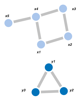
(a)

Figure 8: The set of all fiber bundles $\pi:X\rightarrow Y$ defines an algebraic variety. This variety is given by the Groebner basis (3).

The Pullback Condition reads

$$-1+\alpha_{{4,1}}\alpha_{{5,2}}+\alpha_{{3,1}}\alpha_{{4,2}}+\alpha_{{1,1}}\alpha_{{2,2}}+\alpha_{{3,2}}\alpha_{{4,1}}+\alpha_{{1,2}}\alpha_{{2,1}}+\alpha_{{1,2}}\alpha_{{4,1}}+\alpha_{{2,2}}\alpha_{{3,1}}+\alpha_{{1,1}}\alpha_{{4,2}}+\alpha_{{2,1}}\alpha_{{3,2}}+\alpha_{{4,2}}\alpha_{{5,1}},$$

$$-1+\alpha_{{3,3}}\alpha_{{4,1}}+\alpha_{{1,3}}\alpha_{{2,1}}+\alpha_{{2,3}}\alpha_{{3,1}}+\alpha_{{4,1}}\alpha_{{5,3}}+\alpha_{{1,3}}\alpha_{{4,1}}+\alpha_{{1,1}}\alpha_{{2,3}}+\alpha_{{4,3}}\alpha_{{5,1}}+\alpha_{{2,1}}\alpha_{{3,3}}+\alpha_{{3,1}}\alpha_{{4,3}}+\alpha_{{1,1}}\alpha_{{4,3}},$$

$$-1+\alpha_{{3,3}}\alpha_{{4,2}}+\alpha_{{1,2}}\alpha_{{2,3}}+\alpha_{{1,2}}\alpha_{{4,3}}+\alpha_{{1,3}}\alpha_{{2,2}}+\alpha_{{1,3}}\alpha_{{4,2}}+\alpha_{{2,3}}\alpha_{{3,2}}+\alpha_{{2,2}}\alpha_{{3,3}}+\alpha_{{4,2}}\alpha_{{5,3}}+\alpha_{{3,2}}\alpha_{{4,3}}+\alpha_{{4,3}}\alpha_{{5,2}}.$$

Finally, the Connected Fiber Condition is given by

$$-\alpha_{{1,1}}\alpha_{{2,1}}\alpha_{{5,1}},-\alpha_{{1,1}}\alpha_{{3,1}}\alpha_{{5,1}},-\alpha_{{1,2}}\alpha_{{2,2}}\alpha_{{5,2}},-\alpha_{{1,2}}\alpha_{{3,2}}\alpha_{{5,2}},-\alpha_{{1,3}}\alpha_{{2,3}}\alpha_{{5,3}},-\alpha_{{1,3}}\alpha_{{3,3}}\alpha_{{5,3}}$$

$$-\alpha_{{2,1}}\alpha_{{3,1}}\alpha_{{5,1}},-\alpha_{{2,1}}\alpha_{{4,1}}\alpha_{{5,1}},-\alpha_{{2,2}}\alpha_{{3,2}}\alpha_{{5,2}},-\alpha_{{2,2}}\alpha_{{4,2}}\alpha_{{5,2}},-\alpha_{{2,3}}\alpha_{{3,3}}\alpha_{{5,3}},-\alpha_{{2,3}}\alpha_{{4,3}}\alpha_{{5,3}},$$

$$\quad\alpha_{{2,1}}\alpha_{{5,1}},\alpha_{{2,2}}\alpha_{{5,2}},\alpha_{{2,3}}\alpha_{{5,3}}.$$

A part of the reduced Groebner basis of the resulted system is given by

$$\mathcal{B} = \left\{\beta_{{1}}-1,\beta_{{2}}-1,\beta_{{3}}-1,\beta_{{4}}-1,\beta^{2}_{i}-\beta_{i},\,\alpha_{ij}^{2}-\alpha_{ij},\,\right.$$

$$\alpha_{{1,2}}\alpha_{{1,3}},\alpha_{{1,2}}\alpha_{{3,2}},\alpha_{{1,3}}\alpha_{{3,3}},\alpha_{{2,2}}\alpha_{{2,3}},\alpha_{{2,2}}\alpha_{{4,2}},\alpha_{{2,2}}\alpha_{{5,2}},\alpha_{{2,3}}\alpha_{{4,3}},\alpha_{{2,3}}\alpha_{{5,3}},\alpha_{{3,2}}\alpha_{{3,3}},\alpha_{{4,2}}\alpha_{{4,3}},$$

$$\alpha_{{4,2}}\alpha_{{5,3}},\alpha_{{4,3}}\alpha_{{5,2}},\alpha_{{5,2}}\alpha_{{5,3}},\alpha_{{4,2}}\alpha_{{5,2}}-\alpha_{{5,2}},\alpha_{{4,2}}\beta_{{5}}-\alpha_{{5,2}},\alpha_{{4,3}}\alpha_{{5,3}}-\alpha_{{5,3}},$$

$$\quad\quad\vdots$$

$$-\alpha_{{2,2}}\alpha_{{5,3}}-\alpha_{{3,2}}\alpha_{{5,3}}+\alpha_{{1,2}}\beta_{{5}}+\alpha_{{2,2}}\beta_{{5}}+\alpha_{{3,2}}\beta_{{5}}+\alpha_{{3,3}}\beta_{{5}}+\alpha_{{5,2}}+\alpha_{{5,3}}-\beta_{{5}}\left.\right\}.$$

In particular, the intersection $\mathcal{B}\cap\mathbb{Q}[\beta]=(\beta_{{1}}-1,\beta_{{2}}-1,\beta_{{3}}-1,\beta_{{4}}-1,{\beta_{{5}}}^{2}-\beta_{{5}})$ gives the two $Y$ minors (i.e., subgraphs $X^{\beta}$) inside $X$. The remainder of $\mathcal{B}$ gives the explicit expressions of the corresponding mappings.

4.2.4 Counting embeddings without solving equations

The number of zeros of an ideal $\mathcal{I}\subset\mathbb{Q}[x_{0},\cdots,x_{n-1}]$ can be determined without solving any equation in $\mathcal{I}$. This is done using staircase diagrams, as follows. To each polynomial in $\mathcal{I}$ we assign a point in the Euclidean space $\mathbb{E}^{n}$ given by the exponents of its leading term (with respect to the given monomial order). Figure 9 depicts three staircase diagrams.

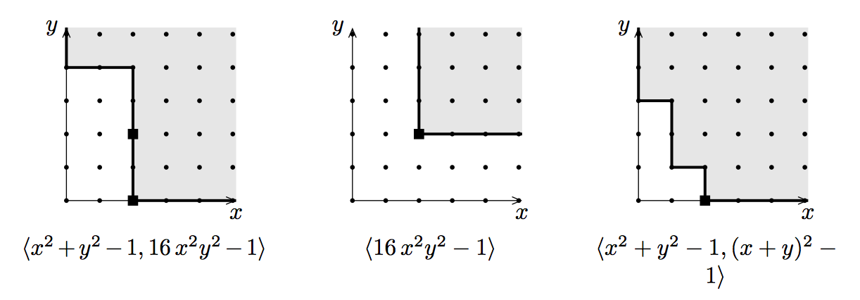
Figure 9: Staircase diagrams of three ideals in $\mathbb{Q}[x,y]$. For these examples, the staircase diagrams are the same for the monomial orders lex, deglex, and degrevlex.

Proposition 6

The ideal $\mathcal{I}\subset\mathbb{Q}[x_{0},\cdots,x_{n-1}]$ is zero dimensional if and only if the number of points under the shaded region of its staircase is finite, and this number is equal to the dimension of the quotient $Q[x_{0},\cdots,x_{n-1}]/\mathcal{I}$, that is, the number of zeros of $\mathcal{I}$.

One can see that the number of zeros of the three ideals in Figure 9 (left to right) are $8,\,\infty$ and 4 respectively.

The application of this construction to the problem of counting all embeddings ${\pi:X\rightarrow Y}$ is obvious. The ideal $\mathcal{I}$ is given by the different requirements on the coefficients $\alpha_{ij}$ of the map $\pi$ as discussed previousely. Note that the dimension of $Q[\alpha,\beta,\delta]/\mathcal{I}$ cannot be infinite because there is (if any) only finite number of possible embeddings. An example is depicted in Figure 10.

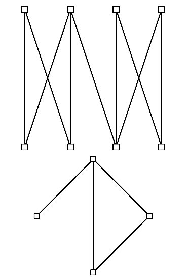
Figure 10: There are 360 embeddings, with chains of size at most 2, for the bottom graph into the upper graph.

4.2.5 Symmetries and invariant coordinates

When determining the surjections $\pi$ (or equivalently, the embeddings $\phi)$, many of the solutions are redundant: they are of the form $\pi\circ\sigma$ with $\sigma\in{\bf Aut}(X)$. This is not desirable because it affects the efficiency of the computations. In this subsection, we discard this redundancy by expressing the problem of finding the fiber bundles $\pi$ in a canonical form, using the invariants of the symmetry (automorphism) $\sigma$. Pictorially, this canonical form is obtained by folding the hardware graph $X$ along the symmetry axis.

The tools and concepts that we have used here are rooted in classical invariant theory; a reference to this fascinating subject is the excellent book [Olv99]. The first of these concepts is the notion of invariance: An invariant of a symmetry $\sigma\in Aut(\mathcal{X})$ of an object $\mathcal{X}$ is a real-valued function $I:\mathcal{X}\rightarrow\mathbb{R}$ that satisfies

$$I(\sigma x)=I(x)$$ (4.30)

for all $x\in\mathcal{X}$; the function $I$ is invariant of a subgroup $G\subseteq Aut(\mathcal{X})$ if and only it is invariant of all $\sigma\in G$. Because the sum and the product of invariants are again invariants, the set of all invariants of $G$ forms an algebra (the algebra of $G-$invariants), denoted $\mathcal{A}^{G}$, and is a subalgebra of the algebra of real-valued functions over $\mathcal{X}$. The algebra of $G-$invariants $\mathcal{A}^{G}$ can be very large. In practice, we don’t compute the entire $\mathcal{A}^{G}$, but instead we compute a complete set of invariants that is a maximal set of invariants that are functionally independent (or algebraically independent in the context of polynomials). Any other $G-$invariant can be written as a function thereof. A useful construction for finite groups is the Reynolds symmetrization operators

$$\varsigma=\sum_{\sigma\in G}\sigma,$$ (4.31)

which projects the algebra of functions over $\mathcal{X}$ to the algebra $\mathcal{A}^{G}$. In other words, for each function $f:\mathcal{X}\rightarrow\mathbb{R}$, the function $\varsigma f:\mathcal{X}\rightarrow\mathbb{R}$ is a $G-$invariant (and if $f$ is already invariant then $\varsigma f=f$). This yields a procedure for constructing invariants of $G$. Furthermore, a set of invariants is functionally independent if their Jacobian matrix has full rank.

In our context of mapping binary optimization problems into quantum hardwares, the space $\mathcal{X}$ is the hardware graph $X$, in which case symmetries are permutations of the vertices. For instance, in the case of the example of Figure 11, the rotation around the edge $(x_{1},x_{2})$ is a symmetry. Additionally, the functions $x_{1},x_{2},x_{3}+x_{4},x_{3}x_{4},x_{5}+x_{6},$ and $x_{5}x_{6}$ are invariants. They form a complete set of invariants for this symmetry . Figure 11 (right) gives the canonical representation of the graph $X$ with respect to its symmetry.

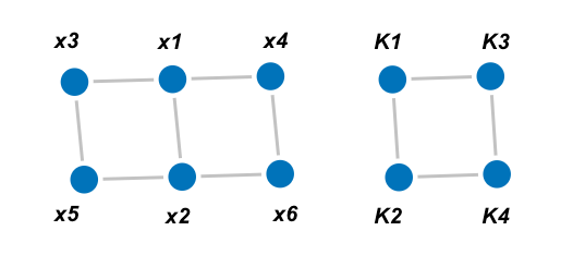
(a)

Figure 11: The hardware graph $X$ (right) is symmetric along the edge $x_{1}x_{2}$. The nodes of the folding (right) correspond to the 4 functionally independent invariants of this symmetry: $K_{1}=x_{1},$ $K_{2}=x_{2},$ $K_{3}=x_{3}+x_{4}$ and $K_{4}=x_{5}+x_{6}$.

In the remainder of this section we explain how this canonical representation can be determined in general. To do so, the notion of “algebra of functions over a graph $X$” needs to be made precise. Indeed, this algebra is the quotient ring:

$$\mathcal{A}_{X}:=\mathbb{Q}[{\bf Vertices}(X)]/\langle\mbox{monomials }x_{i_{1}}x_{i_{2}}|\quad(x_{i_{1}},x_{i_{2}})\notin{\bf Edges}(X)\rangle.$$ (4.32)

Readers familiar with the notion of coordinates rings might notice that $\mathcal{A}_{X}$ is the “coordinates ring” of the complement graph of $X$. Now, suppose $G$ is a subgroup of ${\bf Aut}(X)$ (which is itself a subgroup of the symmetric group $S^{n}$). The set of $G$-invariants forms a subalgebra $\mathcal{A}^{G}_{X}$ of the algebra of functions $\mathcal{A}_{X}$. Folding the graph $X$ along $G$ consists then of applying the following procedure:

• input: A graph $X$ and a complete set of $G-$invariants $\{I_{0}(x),\cdots,I_{r-1}(x)\}$

• output: The folding of $X$ along $G$

• define the system

  $$\mathcal{S}=\{f-Q_{X}(x)\}\cup\{K_{0}-I_{0}(x),\cdots,K_{r-1}-I_{r-1}(x)\}\cup\{x_{i_{1}}x_{i_{2}}|\quad\{x_{i_{1}},x_{i_{2}}\}\notin{\bf Edges}(X)\}.$$

  The system $\mathcal{S}$ is a subset of the extended polynomial ring $\mathbb{Q}[x_{0},\cdots,x_{n-1},K_{0},\cdots,K_{r-1},f]$.

• compute a Groebner basis $\mathcal{B}$ for $\mathcal{S}$ with respect to the monomial order

  $$[x_{0},\cdots,x_{n-1}]\succ f\succ[K_{0},\cdots,K_{r-1}].$$

  The intersection $\mathcal{B}\cap\mathbb{Q}[K_{0},\cdots,K_{r-1},f]$ gives folding of $X$ along $G$.

The use of Groebner bases in this procedure is not a necessity – it is more for conciseness and beauty of the formulation. Another way to do the same task without computing any Groebner basis is by solving the system $\{K_{i}-I_{i}\}$ with respect to the variables $x_{1},\cdots,x_{n}$, replacing the solution in $X$ and then evaluating on the ideal

$${\langle\mbox{monomials }x_{i_{1}}x_{i_{2}}|\quad(x_{i_{1}},x_{i_{2}})\notin{\bf Edges}(X)\rangle}.$$ (4.33)

Let us illustrate this procedure on the example depicted in Figure 11 above. The system $\mathcal{S}$ is given by the polynomials

$${K_{1}}-x_{{1}},\,{K_{2}}-x_{{2}},\,{K_{3}}-x_{{3}}-x_{{4}},\,{K_{4}}-x_{{5}}-x_{{6}},\,{K_{5}}-x_{{3}}x_{{4}},\,{K_{6}}-x_{{5}}x_{{6}},\,$$ (4.34)

$$f-x_{{3}}x_{{1}}-x_{{1}}x_{{4}}-x_{{3}}x_{{6}}-x_{{4}}x_{{5}}-x_{{1}}x_{{2}}-x_{{2}}x_{{6}}-x_{{5}}x_{{2}},\,$$ (4.35)

$$x_{{3}}x_{{4}},\,x_{{5}}x_{{6}},\,x_{{4}}x_{{6}},\,x_{{3}}x_{{5}},\,x_{{1}}x_{{5}},\,x_{{1}}x_{{6}},\,x_{{2}}x_{{4}},\,x_{{2}}x_{{3}}.$$ (4.36)

We compute a Groebner basis $\mathcal{B}$ as in the procedure above. In this case, the intersection $\mathcal{B}\cap\mathbb{Q}[K_{1},\cdots,K_{6},f]$ is the set of polynomials:

$${K_{6}},\quad{K_{5}},\quad{K_{4}}\,{K_{1}},\quad{K_{3}}\,{K_{2}},\quad f-{K_{1}}\,{K_{2}}-{K_{1}}\,{K_{3}}-{K_{2}}\,{K_{4}}-{K_{3}}\,{K_{4}}.$$ (4.37)

The last polynomial gives the rectangular graph of Figure 11 with nodes $K_{1},K_{2},K_{3},$ and $K_{4}$. The example of Figure 12 is treated similarly.

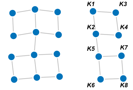
(a)

Figure 12: Folding of the hardware graph $X$ (left) along its symmetry axis. The nodes of the folding (right) are functionally independent invariants of the symmetry.

We finish this subsection with an example illustrating how the embedding is found once redundancy is removed.

Example 4

Consider the two graphs $X$ and $Y$ of Figure 8. The quadratic form of $X$ is:

$$Q_{X}(x)=x_{1}x_{2}+x_{2}x_{3}+x_{3}x_{4}+x_{1}x_{4}+x_{4}x_{5}.$$ (4.38)

Exchanging the two nodes $x_{1}$ and $x_{3}$ is a symmetry for $X,$ and the quantities $K=x_{1}+x_{3},\,x_{2},\,x_{4},$ and $x_{5}$ are invariants of this symmetry. In terms of these invariants, the quadratic function $Q_{X}(x)$, takes the simplified form:

$$Q_{X}(x,K)=Kx_{2}+Kx_{4}+x_{4}x_{5},$$ (4.39)

which shows (as expected) that graph $X$ is folded into a chain (given by $[x_{2},K,x_{4},x_{5}]$). The surjective homomorphism $\pi:X\rightarrow Y$ now takes the form

$$\left\{\begin{array}[]{lll}K&=&\alpha_{01}y_{1}+\alpha_{02}y_{2}+\alpha_{03}y_{3}.\\ x_{i}&=&\alpha_{i1}y_{1}+\alpha_{i2}y_{2}+\alpha_{i3}y_{3}\mbox{ for }i=2,4,5.\end{array}\right.$$ (4.42)

The coefficients $\alpha_{ij}$ for $i=2,4,5$ are constrained as usual. The coefficients $\alpha_{0j}$ are binary subject to $\sum_{j}\alpha_{0j}\leq 2$. In general, if $K=\sum_{i\in I}x_{i}$ where $d(x_{i_{1}},x_{i_{2}})>k$ for all ${i_{1}},{i_{2}}\in I$, then we have $\sum_{j}\alpha_{0j}\leq\mathrm{card}(I)$. The number $k$ is the maximum allowed size of the chains. The table below compares the computations of the surjections $\pi$ with and without the use of invariants:

	original coordinates	invariant coordinates
Time for computing a Groebner basis (in secs)	0.122	0.039
Number of defining equations	58	30
Maximum degree in the defining equations	3	2
Number of variables in the defining equations	20	12
Number of solutions	48	24

In particular, the number of solutions is down to 24, that is, four (non isomorphic) minors times the six symmetries of the logical graph $Y$.

Let us conclude this section by noting that symmetries of the problem graph can also be considered; however, this is problem dependent and needs to be redone if the problem is changed (unlike the hardware graph $X$, which is fixed).

4.3 Analytical dependence of the spectral gap of the adiabatic Hamiltonian on the points of the embedding variety

Consider a hardware graph $X$ and a problem graph $Y$. This section discusses the dependence of the computational complexity of AQC on the choice of the embedding of $Y$ inside $X$.

One of the key findings of this paper is that the set of embeddings $\pi:X\rightarrow Y$ is an algebraic variety i.e., a geometrical object with a coordinate system given by a reduced Groebner $\mathcal{B}$. Our problem translates into determining the algebraic dependence of the computational complexity of AQC on the coordinates of the variety $\mathcal{V}(\mathcal{B})$. That is, determining the algebraic dependence of the spectrum of the adiabatic Hamiltonian

$$H(t)=\alpha(t)H_{initial}+\beta(t)H_{(\mathcal{P})}$$ (4.43)

on the coordinates of the variety $\mathcal{V}(\mathcal{B})$. One way to proceed is to obtain the most general expression of the quadratic form of the $Y$ minor, which we denote by $\tilde{\phi}(Q_{Y})(x)$, in terms of the parameters $\alpha_{ij},$ and $\beta_{i}$ determined by $\mathcal{B}$. This is given by the proposition below, which uses the following observation. Each variable $x_{i}$ can be represented by a row vector $(\alpha_{i1},\cdots,\alpha_{im})\in\{0,1\}^{m}$. In this case, two physical qubits $x_{i_{1}}$ and $x_{i_{2}}$ are chained if and only if their dot product $\sum_{j}\alpha_{i_{1}j}\alpha_{i_{2}j}$ is not equal to zero. Similarly, the qubit $x_{i}$ is selected (i.e., $x_{i}\in support(\pi)$) if and only if $\sum_{j}\alpha_{ij}$ is not zero.

Proposition 7

Given a hardware graph $X$ and a problem graph $Y$. Let $\mathcal{B}$ denote the reduced Groebner basis that gives the set of embeddings $\pi:X\rightarrow Y$. The general form of the quadratic form of the $Y$ minor is given by

$$\tilde{\phi}(Q_{Y})(x) = \sum_{x_{i_{1}}x_{i_{2}}\in{\bf Edges}(X)}{\sf NF}_{\mathcal{B}}\left\{\left(\sum_{j}\alpha_{i_{1}j}\right)\left(\sum_{j}\alpha_{i_{2}j}\right)\right\}{x_{i_{1}}x_{i_{2}}}$$

$$\quad+\quad M\times{\sf NF}_{\mathcal{B}}\left\{\sum_{j}\alpha_{i_{1}j}\alpha_{i_{2}j}\right\}{(1-2x_{i_{1}})(1-2x_{i_{2}})},$$

with $M$ being one (or more) strong ferromagnetic coupling that maintains the chain. Therefore, the problem Hamiltonian is

$$H_{(\mathcal{P})}(\mathcal{B})=\sum_{\mathrm{i}=(\mathrm{i}_{1},\cdots,\mathrm{i}_{n})\in\{0,1\}^{n}}{\sf NF}_{\mathcal{B}}\left\{\tilde{\phi}(Q_{Y})(\mathrm{i})\right\}|\mathrm{i}\rangle\langle\mathrm{i}|$$ (4.45)

given in the computational basis of the Hilbert space ${\mathbb{C}^{2}}^{\otimes n}.$

Recall that the notation ${\sf NF}_{\mathcal{B}}(f)$ stands for the normal formal of the polynomial $f$ with respect to ${\mathcal{B}}$. This is reviewed in the mathematical background section. We conclude with a simple example.

Example 5

Consider the two graphs given by the quadratic functions $Q_{X}(x)=x_{{1}}x_{{2}}+x_{{2}}x_{{3}}$ and $Q_{Y}(y)=y_{{1}}y_{{2}}$. In this case, the reduced Groebner basis (computed using tdeg order) is given by

$$\beta_{{2}}-1,\quad(\beta_{{1}}-1)(\beta_{{3}}-1),\quad{\beta_{{3}}}^{2}-\beta_{{3}},\quad{\beta_{{1}}}^{2}-\beta_{{1}},\,$$

$$\alpha_{{1,2}}\alpha_{{3,2}},\quad\alpha_{{2,1}}+\alpha_{{2,2}}-1,\quad\alpha_{{3,1}}+\alpha_{{3,2}}-\beta_{{3}},\quad\alpha_{{1,1}}+\alpha_{{1,2}}-\beta_{{1}},\quad\alpha_{{1,2}}\beta_{{1}}-\alpha_{{1,2}},\quad\alpha_{{3,2}}\beta_{{3}}-\alpha_{{3,2}},$$

$$\alpha_{{1,2}}\beta_{{3}}+1+\alpha_{{2,2}}\beta_{{3}}-\alpha_{{1,2}}-\alpha_{{2,2}}-\beta_{{3}},\quad\alpha_{{3,2}}\beta_{{1}}-\alpha_{{2,2}}\beta_{{3}}+\alpha_{{1,2}}+\alpha_{{2,2}}-\beta_{{1}},$$

$$\alpha_{{2,2}}\beta_{{1}}+1+\alpha_{{2,2}}\beta_{{3}}-\alpha_{{1,2}}-2\,\alpha_{{2,2}}-\alpha_{{3,2}},\quad\alpha_{{1,2}}\alpha_{{2,2}}+1+\alpha_{{2,2}}\alpha_{{3,2}}-\alpha_{{1,2}}-\alpha_{{2,2}}-\alpha_{{3,2}},$$

$${\alpha_{{1,2}}}^{2}-\alpha_{{1,2}},\quad\quad{\alpha_{{3,2}}}^{2}-\alpha_{{3,2}},\quad{\alpha_{{2,2}}}^{2}-\alpha_{{2,2}}.$$ (4.46)

The first four polynomials give the reduced Groebner basis $\mathcal{B}\cap\mathbb{Q}[\beta_{1},\beta_{2},\beta_{3}]$, which gives the different domains for the projection $\pi$. The general form of $Y$ minor is given by

$$\tilde{\phi}(Q_{Y})(x)=\beta_{{1}}x_{{1}}x_{{2}}+\beta_{{3}}x_{{2}}x_{{3}}+M\left(-1+\beta_{{1}}+\gamma\right)(-2x_{{1}}+1)(-2x_{{2}}+1)+M\left(\beta_{{3}}-\gamma\right)(1-2x_{{2}})(1-2x_{{3}}),$$ (4.47)

with $\gamma=\alpha_{{3,2}}+\alpha_{{2,2}}\beta_{{3}}-2\alpha_{{2,2}}\alpha_{{3,2}}$.

We envision two additional applications of the previous proposition. First, as a sandbox, it can help in building intuition and providing fruitful directions for further investigation through studying small instances in a systematic, principled and comprehensive manner. The second application is specific to the case when one has a structured class of problems where the scaling follows a certain formulaic description. The general pattern of the adiabatic behaviour might emerge from studying small problem instances.

5 Designing Ising Quantum Architectures

A critical milestone in the development of AQC is the design of Ising architectures that can be physically realized and are capable of solving some important, hard problems – for instance, designing architectures optimized for a particular class of problems in machine learning. This is formalized as designing hardware graphs $X$ that satisfy the following:

• The degree of $X$ cannot exceed a limited degree $d$ (imposed by current manufacturing limitations).

• $X$ contains a minor for each graph $Y\in\mathcal{Y}$, where $\mathcal{Y}$ represents a class of problems of interest.

• Each $Y$ minor is explicitly computable.

This problem as described was posed in [Cho11], where the following nomenclature was introduced:

Definition 2

Let $\mathcal{Y}$ be a family of graphs. A graph $X$ is called $\mathcal{Y}-$minor universal if for any graph $Y\in\mathcal{Y},$ there exists a minor embedding of $Y$ in $X$.

At this point, the reader might anticipate that our approach is able to produce such $\mathcal{Y}-$minor universals. Indeed, it is easy to see that the first requirement translates into the condition $\sum_{j}q_{ij}\leq d$, where $(q_{ij})_{1\leq i,j\leq n}$ is the unknown adjacency matrix of $X$. Additionally, if the family $\mathcal{Y}$ is given by a finite number of graphs $Y_{\mu}$ (where $\mu$ belongs to a finite range), then for each graph $Y_{\mu}$, we define the transformation

$$\pi^{\mu}(x_{i})=\sum_{y_{i}\in V(Y_{i})}\alpha^{\mu}_{ij}y_{j},$$ (5.1)

where the binary coefficients are subject to the conditions (4.2.2) for each index $\mu$. These conditions, in addition to the pullback and connected fiber conditions for all $\mu$ as well as the degree condition above, form a system of polynomials $\mathcal{L}\subset\mathbb{Q}[\alpha^{\mu},q]$ that has all information needed to determine the coefficients $q_{ij}$. More precisely, we have

Proposition 8

Let $\mathcal{B}$ be a reduced Groebner basis for the system $\mathcal{L}$ with respect to the elimination order $\{\alpha_{ij}^{\mu}\}\succ\{q_{ij}\}$. The following statements are true:

• the family of graphs $\mathcal{Y}=\{Y_{\mu}\}$ admits a $\mathcal{Y}-$minor universal graph of size $n$ if and only if $1\notin\mathcal{B}$ (the choice of the ordering used is not relevant for this statement).

• if $1\notin\mathcal{B}$, the set of all $\mathcal{Y}-$minor universal graphs of size $n$ is given by the intersection $\mathcal{B}\cap\mathbb{Q}[q_{ij}]$.

• if $1\notin\mathcal{B}$, the embeddings $\pi^{\mu}$ (i.e., the coefficients $\alpha^{\mu}_{ij}$) are also given by $\mathcal{B}$ (as functions of the $q_{ij}$).

It is easy to see that Proposition 8 also holds when the finite family $\mathcal{Y}=\{Y_{\mu}\}$ is replaced with a parametrized family of graphs provided the conditions on the parameters are algebraic: these additional conditions are added to the ideal $\mathcal{L}$, which is now a subset of the polynomial ring $\mathbb{Q}[\alpha^{\mu},q,\mu]$. In this case, we compute a reduced Groebner basis for the system $\mathcal{L}$ with respect to the elimination order $\{\alpha_{ij}^{\mu}\}\succ\{q_{ij}\}\succ\{\mu\}$.

Another possible extension is by combining Proposition 8 with Proposition 7. The latter gives the anlaytical dependance of the spectral gap of the adiabatic Hamiltonian on the the variety $\mathcal{V}(\mathcal{B})=\{\pi:X\rightarrow Y\}$. In Proposition 7, we consider a family $\mathcal{Y}$ of graphs (instead of one graph $Y$). In that case, we obtain the dependence of the spectral gap of $H(t)$ on the choice of the $\mathcal{Y}$ minor universal as well as the different corresponding embeddings.

6 Concluding Remarks

In this paper, we developed a novel algebraic geometry framework to solve integer polynomial optimization using adiabatic quantum computing. Our approach represents the first fully systematic translator for AQC in which the intricate steps in the compiler process are codified algorithmically. This approach can also serve as a test-bed to design scalable compilers (by empirically testing the performance of various embeddings that differ on chain length, number of physical qubits used and other features) and Ising architecture design.

7 Acknoledgements

We thank Jesse Berwald, Denny Dahl and Steve Reinhardt from D-Wave systems who provided insight and expertise. We also thank Eleanor G. Rieffel, Bryan O’Gorman, Davide Venturelli and NASA QuAIL team members for comments and feedback.

References

- [AE99] Joseph E. Avron and Alexander Elgart, Adiabatic theorem without a gap condition, Communications in Mathematical Physics 203 (1999), no. 2, 445–463.
- [AvDK+04] D. Aharonov, W. van Dam, J. Kempe, Z. Landau, S. Lloyd, and O. Regev, Adiabatic quantum computation is equivalent to standard quantum computation, 45th Annual IEEE Symposium on Foundations of Computer Science, Oct 2004, pp. 42–51.
- [Bar82] F Barahona, On the computational complexity of ising spin glass models, Journal of Physics A: Mathematical and General 15 (1982), no. 10, 3241.
- [BF28] M. Born and V. Fock, Beweis des adiabatensatzes, Zeitschrift für Physik 51 (1928), no. 3, 165–180.
- [BH02] Endre Boros and Peter L. Hammer, Pseudo-boolean optimization, Discrete Appl. Math. 123 (2002), no. 1-3, 155–225.
- [BKR16] Tomas Boothby, Andrew D. King, and Aidan Roy, Fast clique minor generation in chimera qubit connectivity graphs, Quantum Information Processing 15 (2016), no. 1, 495–508.
- [BPT00] Dimitris Bertsimas, Georgia Perakis, and Sridhar Tayur, A new algebraic geometry algorithm for integer programming, Management Science 46 (2000), no. 7, 999–1008.
- [CFP01] Andrew M. Childs, Edward Farhi, and John Preskill, Robustness of adiabatic quantum computation, Phys. Rev. A 65 (2001), 012322.
- [Cho08] Vicky Choi, Minor-embedding in adiabatic quantum computation: I. the parameter setting problem, Quantum Information Processing 7 (2008), no. 5, 193–209.
- [Cho11] , Minor-embedding in adiabatic quantum computation: II. minor-universal graph design, Quantum Information Processing 10 (2011), no. 3, 343–353.
- [CLO07] David A. Cox, John Little, and Donal O’Shea, Ideals, varieties, and algorithms: An introduction to computational algebraic geometry and commutative algebra, Springer-Verlag, Berlin, Heidelberg, 2007.
- [CMR14] Jun Cai, William G. Macready, and Aidan Roy, A practical heuristic for finding graph minors, CoRR abs/1406.2741 (2014).
- [CT91] Pasqualina Conti and Carlo Traverso, Buchberger algorithm and integer programming, Proceedings of the 9th International Symposium, on Applied Algebra, Algebraic Algorithms and Error-Correcting Codes (London, UK, UK), AAECC-9, Springer-Verlag, 1991, pp. 130–139.
- [DA17] Raouf Dridi and Hedayat Alghassi, Prime factorization using quantum annealing and computational algebraic geometry, Sci. Rep. 7 (2017).
- [DS98] Persi Diaconis and Bernd Sturmfels, Algebraic algorithms for sampling from conditional distributions, Ann. Statist. 26 (1998), no. 1, 363–397.
- [Fau99] Jean-Charles Faugere, A new efficient algorithm for computing Gröbner bases (F4), Journal of Pure and Applied Algebra 139 (1999), no. 13, 61 – 88.
- [FGG+01] Edward Farhi, Jeffrey Goldstone, Sam Gutmann, Joshua Lapan, Andrew Lundgren, and Daniel Preda, A quantum adiabatic evolution algorithm applied to random instances of an np-complete problem, Science 292 (2001), no. 5516, 472–475.
- [JAG+11] M. W. Johnson, M. H. S. Amin, S. Gildert, T. Lanting, F. Hamze, N. Dickson, R. Harris, A. J. Berkley, J. Johansson, P. Bunyk, E. M. Chapple, C. Enderud, J. P. Hilton, K. Karimi, E. Ladizinsky, N. Ladizinsky, T. Oh, I. Perminov, C. Rich, M. C. Thom, E. Tolkacheva, C. J. S. Truncik, S. Uchaikin, J. Wang, B. Wilson, and G. Rose, Quantum annealing with manufactured spins, Nature 473 (2011), no. 7346, 194–198.
- [JFS06] Stephen P. Jordan, Edward Farhi, and Peter W. Shor, Error-correcting codes for adiabatic quantum computation, Phys. Rev. A 74 (2006), 052322.
- [Kat50] Tosio Kato, On the adiabatic theorem of quantum mechanics, Journal of the Physical Society of Japan 5 (1950), no. 6, 435–439.
- [KN98] Tadashi Kadowaki and Hidetoshi Nishimori, Quantum annealing in the transverse ising model, Phys. Rev. E 58 (1998), 5355–5363.
- [Luc14] Andrew Lucas, Ising formulations of many np problems, Frontiers in Physics 2 (2014), 5.
- [MLM07] Ari Mizel, Daniel A. Lidar, and Morgan Mitchell, Simple proof of equivalence between adiabatic quantum computation and the circuit model, Phys. Rev. Lett. 99 (2007), 070502.
- [Olv99] Peter J. Olver, Classical invariant theory, London Mathematical Society Student Texts, Cambridge University Press, 1999.
- [PS01] Pablo A. Parrilo and Bernd Sturmfels, Minimizing polynomial functions, DIMACS Series in Discrete Mathematics and Theoretical Computer Science (2001).
- [ST97] Bernd Sturmfels and Rekha R. Thomas, Variation of cost functions in integer programming, Math. Program. 77 (1997), 357–387.
- [Stu96] Bernd Sturmfels, Gröbner bases and convex polytopes, University Lecture Series, vol. 8, American Mathematical Society, Providence, RI, 1996. MR 1363949
- [TTN95] Sridhar R. Tayur, Rekha R. Thomas, and N. R. Natraj, An algebraic geometry algorithm for scheduling in presence of setups and correlated demands, Math. Program. 69 (1995), 369–401.