A search for black hole microlensing signatures in globular cluster NGC 6656 (M 22)

Abstract

We report the results of a study aiming to detect signs of astrometric microlensing caused by an intermediate-mass black hole (IMBH) in the center of globular cluster M 22 (NGC 6656). We used archival data from the Hubble Space Telescope (HST) taken between 1995 and 2014, to derive long-baseline astrometric time series for stars near the center of the cluster, using state-of-the-art software to extract high-precision astrometry from images. We then modelled these time-series data, and compared microlensing model fits to simple linear proper-motion fits for each selected star. We find no evidence for astrometric microlensing in M 22, in particular for Bulge stars, which are much more likely to be lensed than cluster stars, due to the geometry of microlensing events. Although it is in principle possible to derive mass limits from such non-detections, we find that no useful mass limits can be derived for M 22 with available data, mostly due to a 10-year gap in coverage. This is a result from difficulties with deriving precise enough astrometry from Wide Field Planetary Camera 2 (WFPC2) observations, for stars that do not fall on the PC chip. However, this study shows that, for other HST instruments, we are able to reach precisions at which astrometric microlensing signals caused by IMBH in globular clusters could be detected, and that this technique is a promising tool to make a first unambiguous detection of an IMBH.

1 Introduction

The formation of supermassive black holes (SMBHs) in the early Universe is one of the most debated issues in modern astronomy. Indeed, SMBHs are found at large redshifts, meaning that some of them had already formed only a few hundred million years after the Big Bang (Fan, 2006). However, this quick formation cannot be explained by accretion alone, since stellar-mass black holes cannot accrete enough matter in such a short time, even at the maximum allowed accretion rate, the Eddington rate. Although super-Eddington accretion might take place via different mechanisms (e.g. Alexander & Natarajan, 2014), the favoured scenario for SMBH formation is instead through the merger of seed intermediate-mass black holes (IMBHs), which themselves may form through runaway mergers of stars.

For this reason, much effort has been devoted in recent years to searching for evidence of the existence of IMBHs, focusing on environments where they might have formed, such as in globular clusters. Besides having high enough stellar densities to form IMBHs, globular clusters have velocity dispersions consistent with a low-mass extrapolation of the M-$\sigma$ relation (e.g. Ferrarese & Merritt, 2000), making them good host candidates for IMBHs. In addition to this, they could also have delivered seed IMBHs to the center of galaxies to form SMBHs, since globular clusters are usually about the same age as their host galaxies.

Kains et al. (2016) proposed using gravitational microlensing to achieve an unambiguous IMBH detection, motivated by hitherto-published detections being subject to strong caveats and possible alternative explanations. Indeed, microlensing by an IMBH in the cluster would produce an astrometric deflection to the position of background stars, which, if detected, would then allow us to derive a mass for the IMBH, without relying on any assumption on the nature of the system. This is an advantage over other techniques; for instance, observations aiming to detect X-ray emission caused by accretion onto an IMBH are reliant on assumed accretion models (Grindlay et al., 2001; Maccarone et al., 2005; Haggard et al., 2013; Mezcua et al., 2015), and cusps in both photometric and kinematic profiles are not unique signature of the presence of an IMBH in the cluster center (Illingworth & King, 1977; Baumgardt et al., 2003; Lanzoni et al., 2007; Ibata et al., 2009; Trenti et al., 2010; Vesperini & Trenti, 2010).

In this paper, we report attempts to detect the astrometric deflection that might be caused by an IMBH in the globular cluster M 22 on background stars, due to gravitational microlensing. M 22 (NGC 6656) was identified by Kains et al. (2016) as the most promising candidate for such a detection, thanks to the combination of a high density of background Galactic Bulge stars, a large cluster-Bulge relative motion, and, at 3.2 kpc, being one of the closest globular clusters in the Milky Way. This makes the detection of an astrometric lensing event more likely to be achievable over reasonable timescales, given their long typical timescales ($\sim 3000$ days for an $10^{4}M_{\odot}$ IMBH).

In Sec. 2, we review the basics of astrometric microlensing, and how a detection of this effect can lead to a direct mass estimate; in Sec. 3, we describe the HST archival data used for this study, and the reduction process. We outline our procedure to model astrometric time series for each star in our sample in Sec. 4, and discuss our results in Sec. 5.

2 Astrometric microlensing

For a full discussion of astrometric microlensing, we refer the reader to Hog et al. (1995) and Dominik & Sahu (2000). Here we recall the key equations that are relevant to the work presented in this paper.

Gravitational microlensing occurs when a background source, located at a distance $D_{\mathrm{S}}$ from the observer, becomes sufficiently aligned with a foreground lens object at distance $D_{\mathrm{L}}$. Given a lens of mass $M$, the Einstein ring radius $\theta_{\mathrm{E}}$ gives a typical angular scale for the alignment necessary for microlensing to occur, and is given as

$$\theta_{\mathrm{E}}=\sqrt{\frac{4GM}{c^{2}}(D_{\mathrm{L}}^{-1}-D_{\mathrm{S}}^{-1})}\,.$$ (1)

Because multiple, non-identical, images of the source are produced during a microlensing event, but these usually cannot be resolved, we can, instead of the motion of individual images, observe the motion of the source’s centroid as the event unfolds. With the source-lens angular separation $u$ expressed in units of $\theta_{\mathrm{E}}$, one can derive an expression for the astrometric shift $\delta(u)$ that occurs during a microlensing event (Hog et al., 1995) as

$$\delta(u)=\frac{u}{u^{2}+2}\theta_{\mathrm{E}}\,.$$ (2)

Note that this expression assumes a dark lens, i.e. no or negligible blended light from the lens. This gives the total deflection caused by microlensing, which points away from the lens, as seen by the observer, i.e. along a line joining the lens and undeflected source positions.

The components parallel and perpendicular to the source-lens relative motion can be expressed (e.g. Dominik & Sahu 2000) as

$$\delta_{\parallel}=\frac{p}{u_{\mathrm{0}}^{2}+p^{2}+2}\theta_{\mathrm{E}}$$

$$\delta_{\perp}=\frac{u_{\mathrm{0}}}{u_{\mathrm{0}}^{2}+p^{2}+2}\theta_{\mathrm{E}}\,,$$ (3)

where $u_{\mathrm{0}}$ is the impact parameter, or minimum source-lens angular separation, in units of $\theta_{\mathrm{E}}$, and $p\equiv p(t)$ is expressed as

$$p=\frac{t-t_{\mathrm{0}}}{t_{\mathrm{E}}}\,,$$ (4)

where $t_{\mathrm{0}}$ is the time at which $u=u_{\mathrm{0}}$, $t_{\mathrm{E}}$ is the Einstein timescale, defined as the time taken by the source to cross $\theta_{\mathrm{E}}$. In two dimensions, a source affected by microlensing traces an elliptical motion, in the source’s rest frame, and relative to its undeflected position, with eccentricity $\epsilon=[2/(u_{0}^{2}+2)]^{1/2}$ (Dominik & Sahu, 2000).

From Eq. (1), we see that the mass of the lens, $M$, can be measured directly if three quantities are determined: the distances to the source and lens, $D_{\mathrm{S}}$ and $D_{\mathrm{L}}$, and $\theta_{\mathrm{E}}$. Although the lens distance is usually unknown in microlensing events, and can only be constrained when second-order effects can be measured from photometric light curves, such as the parallax effect caused by the Earth’s orbit around the Sun (e.g. Dominik, 1998; An et al., 2002; Gould, 2004), in the case of an IMBH in the center of a globular cluster, $D_{\mathrm{L}}$ is known, to the extent that the distance to the cluster is known. For Galactic globular clusters, this is usually the case to a precision of a few hundred parsecs (e.g. Harris, 1996).

The discussion above assumes that the images are unresolved. However, when considering IMBH lenses, with possible values of $\theta_{\mathrm{E}}$ of several hundreds of mas for the top end of the IMBH mass range ($>10^{5}M_{\odot}$), it is possible that some events may fall in the “partially-resolved” regime. In this case, the separation between the source images is large enough to be resolved with instruments on HST, and Eq. (2) becomes instead

$$\delta(u)_{pr}=\frac{1}{2}(\sqrt{u^{2}+4}-u)\theta_{\mathrm{E}}\,.$$ (5)

For values of $u\gtrsim 4$, Equations 2 and 5 converge. In the following discussion of our data and modelling procedure, we will show that here we can safely assume that stars in the unresolved microlensing regime.

3 Data and reduction process

3.1 Archival data

We searched the Mikulski Archive for Space Telescopes (MAST) for data that would satisfy several criteria. Images must have been observed in medium- or wide-band filters, with the Wide Field Planetary Camera 2 (WFPC2), the Advanced Camera for Survey (ACS)’s, or Wide Field Camera 3 (WFC3); this is because observations taken with narrow-band filters do not go deep enough to enable us to derive precise astrometry for Bulge stars. Images must also contain the center of M 22 at least 10^′′ from the edge of the image, and have exposure times long enough to probe background Bulge stars located behind the cluster. A summary of the final data set satisfying these criteria, spanning 19.33 years, is given in Table 1.

Proposal ID	PI	Instrument/ Camera	Dates	Filters	Exposure times
5344	Bailyn1	WFPC2/PC	March 1995	F439W	40-400s
				F675W	10-100s
*7615	Sahu2	WFPC2/WFC	March-June 1999	F606W	260s
			March 1999 - February 2000	F814W	260s
*8174	Van Altena	WFPC2/WFC	June 2000	F555W	26s
10524	Ferraro	WFPC2/PC	April 2006	F555W	30s
10775	Sarajedini3	ACS/WFC	April 2006	F606W	55s
				F814W	65s
*11233	Piotto4	WFPC2/WFC	April 2008	F450W	350s
				F814W	100s
11975	Ferraro	WFPC2/PC	April 2009	F555W	10s
12193	Lee	WFC3/UVIS	May 2011	F467M	361-367s
				F547M	75s
12311	Piotto5	WFC3/UVIS	Sept 2010 - March 2011	F275W	812s
				F814W	50s
13297	Piotto5	WFC3/UVIS	July 2014	F336W	475s
				F438W	141s

Table 1: HST archival data of M 22 that satisfied our observing criteria. An asterisk in front of the program number denotes WFPC2 data sets which we subsequently excluded (see text). Reference papers describing the observing programs in detail, when available, are: ¹Bailyn et al. (1996); ²Sahu et al. (2001); ³Sarajedini et al. (2007); ⁴Piotto et al. (2012); ⁵Piotto et al. (2015).

3.2 Reduction

We reduced available images from data sets given in Table 1 using the suite of tools developed by Jay Anderson (e.g. Anderson & King, 2003). For ACS and WFC3 images, we used flc images, which are available in the archive, and have been corrected for charge-transfer efficiency (CTE) losses. The importance of CTE loss correction has been discussed in several papers; for more details, see e.g. Bellini et al. (2014).

The first detection and measurement of stars in each image was made using the routine hst1pass. When available, a standard PSF array was used for each instrument/ filter combination Anderson & King (2006); when these were not available, we used the available standard PSF that was closest in wavelength (e.g. for the F547M filter, we used the F467M standard PSF). This is satisfactory because the PSF that is used for the measurement of each star is actually an interpolation of the nearest four PSFs on the image. Furthermore, the time dependence is also accounted for by calculating perturbations to the PSF for each observation. Finally, we also applied the geometric distortion corrections of Anderson & King (2006) to position measurements.

Using an image from the ACS Survey of Galactic Globular Clusters (HST Treasury Program, Sarajedini et al. 2007) as a reference, we used xym2mat to derive positions in a common coordinate system of all stars in each image. This is done by deriving a 6-parameter transformation between an image and the reference, allowing us to measure the position of stars on each transformed image. Applying this transformation to the entire set of available images then yields astrometric time series for each star.

Although transformations were derived for WFPC2/WFC images, these were found to be imprecise, with scatter as large as 1 pixel in most measurements. There are several reasons for this: WFPC2’s larger pixels, its smaller dynamic range, and the lack of dithering typical of early HST observations. Due to this, we did not include WFPC2/WFC images in the rest of the analysis. This issue did not affect the planetary camera (PC) on WFPC2, and we retain these data for further analysis, in addition to ACS and WFC3 data. The excluded data sets were those of proposal ID 7615 (PI: Sahu), 8174 (PI: Van Altena), and 11233 (PI: Piotto).

3.3 Proper motion corrections

Cluster stars are extremely unlikely to be lensed by another object in the cluster, since for such a case, $D_{\mathrm{S}}/D_{\mathrm{L}}\sim 1$, resulting in a very small Einstein ring radius (Eq. 1). We can therefore assume that cluster stars move in a straight lines, i.e. without any microlensing deflections, and use this to correct for systematics that may result in non-rectilinear time series for those stars.

To do this, we fitted straight-line proper motions to the time series of all cluster stars, and looked at the distribution of residuals from those fits. For each filter/ epoch/ instrument, we then computed the median residual from the straight-line fit. In case systematics offsets are present, these median residuals would be nonzero, whereas for random scatter, the distribution of residuals would be centered on zero. For each filter/ epoch/ instrument, we then subtracted this median offset value from the time series of all stars. We binned data taken with the same instrument in 10-day bins; given the very slow-evolving signals we are looking for in this work, any variation that may happen on 10-day timescales can be ignored without losing significant information on the long-timescale events. Finally, position measurements for different filters were combined at each epoch, producing a single position at each epoch/ instrument combination.

3.4 Stars near the center

We used the center coordinates for the cluster center from Goldsbury et al. (2010), $\alpha=18.36.23.94,\delta=-23:54:17.10$; associated uncertainties are $\pm 0.8^{\prime\prime}$. Although any IMBH present in the cluster is expected to be located at the center, $N-$body simulations suggest that it might also be slightly off-center due to interactions between the IMBH and stars in the cluster (de Vita et al., 2018). We therefore selected stars within a radius of 6^′′ of the center for further analysis, in order to be conservative in accounting both for uncertainties in the precise location of the center itself, and for the amount by which an IMBH might be off-center (de Vita et al., 2018).

The large M 22-Bulge relative motion of $\sim 12.2$ mas yr^-1 (Kains et al., 2016; Bellini et al., 2014) makes cluster members easily distinguishable from background Bulge stars using their proper motion, derived from initial linear fits to their astrometric time series, as shown in Fig. 1. Using this, we identified 8 Bulge stars from 199 stars detected on the reference image within 6^′′ of the center. Coordinates and proper motions for these 8 stars are given in Table 2

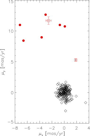
Figure 1: Proper motions derived from initial straight-line fits to astrometric time series. Cluster stars are shown as open diamonds, while Bulge stars, clearly separated in the proper motion diagram, are plotted as filled red circles and open squares (for the two stars with $<4$ epochs with astrometric measurements), with 1-$\sigma$ error bars (too small to see for most stars).

Star	RA	Dec	$\mu_{x}$	$\mu_{y}$	$N_{e}$
	(J2000.0)	(J2000.0)	[mas yr-1]	[mas yr-1]
1	18:36:24.19	-23:54:18.19	-0.72$\pm$0.02	10.97$\pm$0.03	8
2	18:36:24.43	-23:54:20.52	-3.67$\pm$0.12	8.96$\pm$0.02	5
3	18.36:24.35	-23:54:14.04	-7.19$\pm$0.02	10.97$\pm$0.08	6
4	18:36:24.24	-23:54:12.60	-2.56$\pm$0.43	11.68$\pm$0.61	3
5	18:36:24.22	-23:54:18.30	-6.62$\pm$0.04	8.42$\pm$0.02	6
6	18:36:24.13	-23:54:15.00	1.85$\pm$0.07	5.28$\pm$0.19	4
7	18:36:23.88	-23:54:18.27	-3.03$\pm$0.03	12.64$\pm$0.05	7
8	18:36:23.87	-23:54:19.19	0.09$\pm$0.05	10.73$\pm$0.04	8

Table 2: Coordinates, proper motions (along the $x$ and $y$ image directions), and number of epochs with astrometric measurements for the 8 Bulge stars in our sample within 6^′′ of the cluster center.

4 Modelling procedure

For each star in our sample, we fitted two models:

1. A proper-motion (PM)-only model, with parameters $\mu_{x},\mu_{y},x_{0}$, and $y_{0}$, respectively the proper motions along the $x$ and $y$ directions on the image, and arbitrary reference $x$ and $y$ positions

2. An astrometric microlensing (ML) model, described by the standard microlensing parameters $t_{\mathrm{0}},t_{\mathrm{E}},u_{\mathrm{0}}$, described in Sec. 2, as well as $\alpha$, the relative angle of the lens-source trajectories, the Einstein ring radius $\theta_{\mathrm{E}}$, as well as the proper motion parameters $\mu_{x},\mu_{y},x_{0}$, and $y_{0}$.

Note that the closest star to the cluster center is $\sim 1.6^{\prime\prime}$ away from the center coordinates of Goldsbury et al. (2010), which means that any microlensing event would either occur in the unresolved regime, or be very well approximated by unresolved microlensing models, as long as the Einstein ring radius is less than $\sim 400$ mas, which, for a lens in M 22 and a Bulge source, corresponds to a $\sim 10^{5}M_{\odot}$ IMBH. We also note here that in the following discussion, we use the term “shift” when referring to microlensing fits, and “residuals” when referring to residual positions after subtraction of a proper motion model.

After fitting both the PM and ML models, we compared them using the Bayesian Information Criterion (BIC, Schwarz 1978), defined as

$$\mathrm{BIC}=-2\ln(\mathcal{L})+N_{\rm P}\ln(N_{\rm D})\,-N_{\rm P}\ln(2\pi)\,,$$ (6)

where $\mathcal{L}$ is the likelihood, $N_{\rm D}$ is the number of data points (twice the number of epochs, with astrometric measurements, since the position is measured in two directions), and $N_{\rm P}$ is the number of model parameters (9 for ML models, 4 for PM models). Here we have assumed constant priors on most parameters, as no information is available from a photometric microlensing light curve fit, for instance (e.g. Kains et al., 2017) . However, we do impose a Gaussian prior on the relative source-lens motion, using the cluster-Bulge relative motion $12.2\pm 3.9$ mas yr^-1 measured by Kains et al. (2016) from the proper motion catalogue of Bellini et al. (2014). This is particularly important in cases where data are limited, in which case model fits may converge to parameters that are not consistent with the observed relative motion. Using the BIC for the best-fit MCMC models, we then compute their relative probability,

$$\frac{P(\mathrm{PM})}{P(\mathrm{ML})}=\exp(0.5(\mathrm{\Delta_{\mathrm{BIC}})})\,,$$ (7)

where $\Delta_{\mathrm{BIC}}=\mathrm{BIC_{ml}}-\mathrm{BIC_{pm}}$. In addition, we impose an additional requirement that an astrometric lensing be at least 1000 times more probable to be favoured, which corresponds to a threshold $\Delta_{\mathrm{BIC}}$=13.82. The BIC is usually most appropriate when $N_{\rm D}>>N_{\rm P}$, but the high additional penalty we impose on the ML models means that even with a relatively small number of data points, the BIC is sufficient for the purposes of selecting a model in this work. To test this, we generated PM-only astrometric time-series, with scatter corresponding to our real data, and fitted both PM and ML models to these simulated data sets. We generated and fitted 1000 such data sets, and found that with such a strict penalty on the ML models, the “false alarm” rate, i.e. the fraction of these events where the ML model is favored over the correct PM model, is negligible ($<0.1\%$).

Since good astrometry could not be extracted from WFPC2/WFC data, this left us with significant gaps in the time series, and only 8 distinct epochs. To assess whether such coverage would be sufficient to recover lensing parameters, we generated synthetic astrometric time series from a set of input parameters (IMBH mass, source-lens relative motion, microlensing impact parameter). We assumed Gaussian errors on astrometric measurements and scatter consistent with our real data. We then analyzed these synthetic data sets with our modelling codes, and found that synthetic astrometric curves allowed us to recover input parameters for a wide range of masses, although with large associated uncertainties, as expected with this few epochs. Fig. 2 shows an illustration of one such a fit, for a $10^{3}M_{\odot}$ IMBH, with $t_{\mathrm{E}}=1900$ d. However, we do find that this time coverage would miss many events caused by low-mass ($\lesssim 5\times 10^{2}M_{\odot}$) or very high-mass ($\gtrsim 10^{5}M_{\odot}$), due to their short timescales (most of the event happening in coverage gaps) or inability to distinguish the total motion from PM-only motion, respectively.

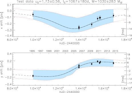
Figure 2: Best-fit model to test data for a $10^{3}M_{\odot}$ IMBH in M 22, with $t_{\mathrm{E}}=1900$ d, $u_{\mathrm{0}}=1.5$. The source-lens relative motion is $\sim 14$ mas yr^-1. Recovered parameters are in agreement with input parameters, but with large error bars. Blue shaded areas and red dotted lines show the limits of the 99.7% confidence interval. The top axis in the bottom panel gives the time in calendar years.

5 Results and discussion

As expected, all cluster stars are found to be consistent with rectilinear, constant proper-motion-only models. Given the cluster distance of 3.2 kpc, parallax shifts of $\sim 0.3$ mas are present in the astrometry, corresponding to variations of $\sim 0.6\%$ of a pixel. This is smaller than the astrometric precision we achieve in this study, and we can therefore safely conclude that parallax does not have a significant effect on our results.

Out of 8 Bulge stars, 2 had insufficient ($<4$) epochs with astrometric measurements, due to their close proximity to saturated stars in most images. This leaves 6 Bulge stars with enough data (5-8 epochs) to detect an astrometric microlensing signal. The lensing model is not favoured over the proper-motion-only model for any of these 6 Bulge stars.

In Fig. 3, we show plots of the time series for the closest star to the center position of Goldsbury et al. (2010), in 2-dimensions with the proper motion subtracted, and of the motion in each of the $x$ and $y$ direction, along with the best-fit proper-motion and lensing models.

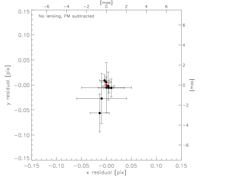
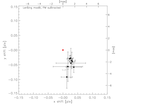
Figure 3: 2-D residual positions after proper motion subtraction, for the PM-only model (top) and astrometric microlensing model (bottom), for the closest star to the center of M 22.

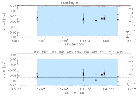
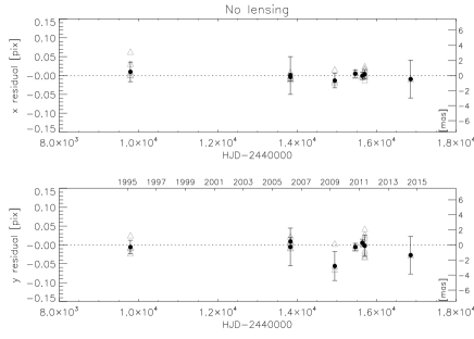
Figure 4: Residual positions after proper motion subtraction, for each of the $x$ and $y$ pixel positions, for the PM-only model (top) and astrometric microlensing model (bottom), for the closest star to the center of M 22. For the microlensing model, the best-fit model to the microlensing shift over the 19.33 year baseline is also plotted as a solid line, and blue shaded areas and red dotted lines show the limits of the 99.7% confidence interval. For each model, a time axis in calendar years is shown between the two panels. Individual-image measurements are shown as grey open triangles, while combined measurements are plotted as filled circles with error bars.

From Figs. 3-4, it is clear that the data is consistent with no microlensing deflection taking place. The PM-only model is strongly favoured, and the microlensing fits converge toward very slow-evolving models, which are essentially indistinguishable from PM-only models. These plots are representative of all 6 Bulge stars in our sample.

Although the 10-year gap in our data coverage does not allow us to place strong limits, can we exclude part of the IMBH mass range, based on the lack of detection of an astrometric lensing signal in those 6 stars? From McLaughlin & van der Marel (2005), the larger estimate for the total mass of M 22 is $\log_{10}(M_{\mathrm{tot}}/M_{\odot})\approx 5.64\pm 0.05$. Therefore an extreme scenario in which an IMBH makes up $\sim 10\%$ of the total cluster mass would mean an IMBH with $\log(M_{\mathrm{tot}}/M_{\odot})\approx 4.64$. How far down the IMBH mass range would a black hole (BH) have caused a detectable event, given our data?

To estimate this, we carried out Monte Carlo simulations, first placing a BH at a location near the center, with variation in the BH location given due to the uncertainty in the precise location of the center (Goldsbury et al., 2010), as well as potential IMBH ”wander”, the size of which goes as $M_{\mathrm{BH}}^{-0.44}$ (de Vita et al., 2018). Given a BH position, the actual location of a Bulge star at observed times, as well as the star’s observed motion relative to the cluster (and thus BH), we then derived lensing parameters. Using these, we calculated the expected astrometric deflection at each observed epoch, and determined whether such a deflection would have been detected, given our astrometric measurements.

If so, our data allows us to exclude the presence of such a BH at the center of M 22. This was repeated for $10^{5}$ random BH locations and masses, after which we calculated the detection rate as a function of BH mass, giving us an estimate of the maximum BH mass that would have produced a given detection rate. This is plotted in Fig. 5 for the closest star to the cluster center. For that star, the detection rate rises steadily as a function of mass, due to the small impact parameter, meaning that high-mass BH events would have been detected despite unfolding slowly. A 50% detection rate corresponds to a BH mass of $\sim 22\%$ of the total cluster mass, while for a BH mass of 10% and 1% of the cluster mass, the detection rates would be $\sim$16% and 2%, respectively. Finally, we also estimated the detection rates, adding a data point every two years over our coverage gap (1996-2005), with an error bar corresponding to the median error in our data set, and Gaussian scatter around a straight-line source trajectory, to assess the improvement from having better time coverage. For the simulated data sets, we find a 50% detection rate at M$\sim$0.12$M_{\rm cluster}$, as well as 42% and 2% for BH masses of 10% and 1% of the total cluster mass, respectively. As expected, more regular time coverage improves detection rates significantly for higher masses ($\gtrsim 10^{4}M_{\odot}$), whereas more frequent observations are needed to improve detection rates at lower masses ($\lesssim 10^{4}M_{\odot}$).

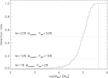
Figure 5: Detection rates as a function of BH mass, given the actual astrometric time-series data, for the star closest to the center of M 22. The vertical dotted red line shows the total cluster mass from McLaughlin & van der Marel (2005), while horizontal lines show detection rates of 50%, as well as for masses corresponding to 10% and 1% of the total cluster mass. Note that an event being detected does not mean that the lens mass can be recovered; see Fig. 6 for an estimate of the probability of events being detected and have the BH mass recovered.

In addition to detecting an event caused by the presence of the BH in the cluster, how often can we also recover the mass of the BH, given our time sampling? We can use simulated data (e.g. Fig. 2) to estimate how the mass recovery rate changes with BH mass, assuming the time coverage of our data set. We did this by generating synthetic data sets, fitting these with our astrometric modelling code, and comparing the fitted parameters to the input parameters. In this case, we considered the mass recovered when the fitted mass was within 0.5 dex of the input mass. In Fig. 6, we plot the mass recovery rate, detection rate, and the multiplication of these two, giving the rate of events that are detected and for which the mass is recovered. We find that given our data, only BH with masses between $10^{4}$ and $10^{5}M_{\odot}$ have a significant chance of both being detected and have their mass recovered, between $\sim$ 3 and 6%. This is because higher-mass events, while they can be detected because of the large signal they produce, are slow-evolving, leading to mostly rectilinear deflections on timescales of $\sim$years; these do not provide good constraints on the lens masses. On the other hand, lower-mass events can be better modeled thanks to less rectilinear deflection signals, but are less easily detected because of the smaller signals they produce.

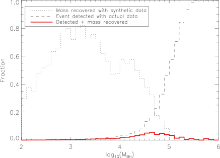
Figure 6: Mass recovery rate (dotted line), detection rate (dashed line), and the product of these two, giving the rate of events that are detected and have their BH mass recovered, as a function of BH mass.

Finally, we checked the catalogue from the Gaia (Gaia Collaboration et al., 2016) data release 2 (DR2, Gaia Collaboration et al. 2018) for matches to the Bulge stars in our sample, to compare our derived proper motions with DR2 values. Indeed, in the most extreme cases involving a background star being deflected by a very massive BH, with a low impact parameter, a trajectory might appear rectilinear over even a 20-year baseline, but could actually be a small fraction of a lensing event. In such a case, the true direction of the star’s proper motion would be different from that derived from the observations, and a second set of later observations might reveal a change in direction, hinting at possible microlensing taking place. Although this would be unlikely to be seen from Gaia data, since they only span 22 months of data from July 2014 to May 2016, whereas our archival data set ends in 2014, we considered this possibility for thoroughness. Unfortunately, only three of our Bulge sources had Gaia matches at a distance $<1^{\prime\prime}$, and none of these 3 had proper motion values in DR2. However, this is a check worth making when considering the possibility of astrometric microlensing by very massive BHs.

6 Conclusions

Using HST archival data spanning nearly 20 years of baseline, we derived astrometric time series for 199 stars within 6^′′ of the center of M 22, but with a large 10-year gap, due to being unable to extract high-precision astrometry from the WFC chips of the WFPC2 instrument. This includes 6 Bulge stars with sufficient time coverage to detect microlensing signals, if present, and constrain the lens properties. These 6 stars do not show any signatures of microlensing deflections, and are consistent with proper-motion-only models. Although in theory it is possible to use these non-detections to place limits on the mass of any IMBH present at the cluster center, the insufficient precision of WFPC2/ WFC astrometry led to a large gap in time coverage that meant we were unable to derive any useful limits for realistic BH masses.

We conclude that it is worth extending this work to other clusters, particularly those with rich HST archival data sets, such as M 4 or 47 Tuc. The tools developed in this study will make future analyses of other clusters much faster. In addition, the astrometric microlensing analysis tools we wrote as part of this project would also be useful in preparation for the Wide Field Infrared Survey Telescope (WFIRST)’s Microlensing Survey, for which astrometry has the potential to significantly improve the constraints yielded by the survey on lens masses (Gould & Yee, 2014), including on the mass function of stellar-mass BHs and extrasolar planets. In addition, it will be worth revisiting models in the future, for instance after observations of the centers of these clusters have been taken by the James Webb Space Telescope (JWST), which will afford even better astrometric precision than what is currently achievable with HST.

References

- Alexander & Natarajan (2014) Alexander, T., & Natarajan, P. 2014, Science, 345, 1330
- An et al. (2002) An, J. H., Albrow, M. D., Beaulieu, J.-P., et al. 2002, ApJ, 572, 521
- Anderson & King (2003) Anderson, J., & King, I. R. 2003, AJ, 126, 772
- Anderson & King (2006) —. 2006, ACS/ISR 2006-01 (Baltimore, MD: STScI), available online at http://www.stsci.edu/hst/acs/documents/isrs
- Bailyn et al. (1996) Bailyn, C. D., Rubenstein, E. P., Slavin, S. D., et al. 1996, ApJ, 473, L31
- Baumgardt et al. (2003) Baumgardt, H., Hut, P., Makino, J., McMillan, S., & Portegies Zwart, S. 2003, ApJ, 582, L21
- Bellini et al. (2014) Bellini, A., Anderson, J., van der Marel, R. P., et al. 2014, ApJ, 797, 115
- de Vita et al. (2018) de Vita, R., Trenti, M., & MacLeod, M. 2018, MNRAS, 475, 1574
- Dominik (1998) Dominik, M. 1998, A&A, 330, 963
- Dominik & Sahu (2000) Dominik, M., & Sahu, K. C. 2000, ApJ, 534, 213
- Fan (2006) Fan, X. 2006, New Astr. Rev., 50, 665
- Ferrarese & Merritt (2000) Ferrarese, L., & Merritt, D. 2000, ApJ, 539, L9
- Gaia Collaboration et al. (2018) Gaia Collaboration, Brown, A. G. A., Vallenari, A., et al. 2018, ArXiv e-prints, arXiv:1804.09365
- Gaia Collaboration et al. (2016) Gaia Collaboration, Prusti, T., de Bruijne, J. H. J., et al. 2016, A&A, 595, A1
- Goldsbury et al. (2010) Goldsbury, R., Richer, H. B., Anderson, J., et al. 2010, AJ, 140, 1830
- Gould (2004) Gould, A. 2004, ApJ, 606, 319
- Gould & Yee (2014) Gould, A., & Yee, J. C. 2014, ApJ, 784, 64
- Grindlay et al. (2001) Grindlay, J. E., Heinke, C., Edmonds, P. D., & Murray, S. S. 2001, Science, 292, 2290
- Haggard et al. (2013) Haggard, D., Cool, A. M., Heinke, C. O., et al. 2013, ApJ, 773, L31
- Harris (1996) Harris, W. E. 1996, AJ, 112, 1487
- Hog et al. (1995) Hog, E., Novikov, I. D., & Polnarev, A. G. 1995, A&A, 294, 287
- Ibata et al. (2009) Ibata, R., Bellazzini, M., Chapman, S. C., et al. 2009, ApJ, 699, L169
- Illingworth & King (1977) Illingworth, G., & King, I. R. 1977, ApJ, 218, L109
- Kains et al. (2016) Kains, N., Bramich, D. M., Sahu, K. C., & Calamida, A. 2016, MNRAS, 460, 2025
- Kains et al. (2017) Kains, N., Calamida, A., Sahu, K. C., et al. 2017, ApJ, 843, 145
- Lanzoni et al. (2007) Lanzoni, B., Sanna, N., Ferraro, F. R., et al. 2007, ApJ, 663, 1040
- Maccarone et al. (2005) Maccarone, T. J., Fender, R. P., & Tzioumis, A. K. 2005, MNRAS, 356, L17
- McLaughlin & van der Marel (2005) McLaughlin, D. E., & van der Marel, R. P. 2005, ApJS, 161, 304
- Mezcua et al. (2015) Mezcua, M., Roberts, T. P., Lobanov, A. P., & Sutton, A. D. 2015, MNRAS, 448, 1893
- Piotto et al. (2012) Piotto, G., Milone, A. P., Anderson, J., et al. 2012, ApJ, 760, 39
- Piotto et al. (2015) Piotto, G., Milone, A. P., Bedin, L. R., et al. 2015, AJ, 149, 91
- Sahu et al. (2001) Sahu, K. C., Casertano, S., Livio, M., et al. 2001, Nature, 411, 1022
- Sarajedini et al. (2007) Sarajedini, A., Bedin, L. R., Chaboyer, B., et al. 2007, AJ, 133, 1658
- Schwarz (1978) Schwarz, G. 1978, Ann. Statist., 21, 461
- Trenti et al. (2010) Trenti, M., Vesperini, E., & Pasquato, M. 2010, ApJ, 708, 1598
- Vesperini & Trenti (2010) Vesperini, E., & Trenti, M. 2010, ApJ, 720, L179