Compartmental Spatial Multi-Patch Deterministic and Stochastic Models for Dengue

Abstract

Dengue is a vector-borne viral disease increasing dramatically over the past years due to improvement in human mobility. The movement of host individuals between and within the patches are captured via a residence-time matrix. A system of ordinary differential equations (ODEs) modeling the spatial spread of disease among the multiple patches is used to create a system of stochastic differential equations (SDEs). Numerical solutions of the system of SDEs are compared with the deterministic solutions obtained via ODEs.

1 Introduction

With about 390 million dengue cases causing 12,000 deaths per year [14], Dengue fever became an international health threat in many tropical and subtropical countries. The disease dynamics are well known to be particularly complex with large fluctuations of disease incidences.

The vectors are assumed to be located in the residing patch while the human population commutes between the different patches. Throughout the paper, isolated areas of interest will be called as patches and in epidemiology, patches may refer to cities, countries, islands or health districts, like hospital districts and give a coarse spatial information about the disease spread. In this paper, deterministic and stochastic models are presented and the mean numerical solutions of the stochastic model over large number of realizations are compared with the deterministic model dynamics. Throughout this work, only one strain of the Dengue virus is studied and further, studies can be extended to the rest of the virus serotypes  [8]. Note that the model can be without further adaption be applied to graphs.

The paper is organized as follows: Following the introduction, deterministic and stochastic multi-patch models are described. Finally, two numerical examples are carried out to compare the deterministic and stochastic solutions of single patch model and two-patch model.

2 Deterministic Multi-patch Vector Host Models

In this section a multi-patch dengue transmission Host-Vector model is introduced to examine the effect of host movement on dengue transmission dynamics. It is assumed that the patches will have a grid structure and the patch will be specified by the index $i$. There will be $n$ patches under consideration and the patches are coupled with the mobility of the hosts from one to the other. An assumption is made that the vectors do not move between the patches  [14, 6, 7] and the short term movement between the patches are coupled by a residence-budgeting time matrix $P=(p_{ij})_{n\times n}$ for $i,j=1,2,...,n$, where $p_{ij}\in[0,1]$ and $\sum_{j=1}^{n}p_{ij}=1$  [5]. The variables for the model corresponding to a specific patch denoted by $i$ are as follows: susceptible hosts $S_{i}$, infected hosts $I_{i}$, and infected vectors $V_{i}$ which is an extension of the model [10] and further, the model used here is an reduction of the model  [2] assuming that the system is conservative. Both the host and vector populations ($N$ and $M$) are considered to be constant. Dengue fever is assumed to be transmitted by two means of interactions between host and vector: susceptible mosquitoes $(U_{i})$ may interact with infected human $(I_{i})$ individuals at a rate of $\frac{\vartheta_{i}}{N_{i}}$ and infected mosquitoes $(V_{i})$ may interact with susceptible humans $(S_{i})$ at a rate of $\frac{\beta_{i}}{M_{i}}$. The incidence rates at which humans and mosquitoes get infected are $\frac{\beta_{i}}{M_{i}}S_{i}V_{i}$ and $\frac{\vartheta_{i}}{N_{i}}U_{i}I_{i}$, respectively. The birth and death rate of the humans is denoted by $\mu_{i}$ , and it is assumed that the renovation of population happens in every 69 years  [12]. The average time taken to recover is considered to be $\gamma_{i}$ and $\nu_{i}$ is the birth and death rate of the mosquitoes. Furthermore, it has been taken into account that the fact $S_{i}+I_{i}+R_{i}=N_{i}$ and $U_{i}+V_{i}=M_{i}$ and then the reduced system of nonlinear ordinary differential equations for the $n$ number of patches are as follows:

$${\dot{\bf{S_{i}}}} = -S_{i}\sum_{j=1}^{n}\frac{\beta_{j}}{M_{j}}p_{ij}V_{j}+\mu_{i}(N_{i}-S_{i})$$

$${\dot{\bf{I_{i}}}} = S_{i}\sum_{j=1}^{n}\frac{\beta_{j}}{M_{j}}p_{ij}V_{j}-(\mu_{i}+\gamma_{i})I_{i}$$

$${\dot{\bf{V_{i}}}} = \frac{\vartheta_{i}}{N_{i}}(M_{i}-V_{i})\sum_{j=1}^{n}p_{ji}I_{j}-\nu_{i}V_{i}$$ (1)

The basic reproductive number, $\mathbf{R}_{0}$ is the average number of secondary infectious cases when a single infectious individual is introduced into the whole susceptible population. The disease dies out if the basic reproduction number $\mathbf{R}_{0}<1$, and disease persists whenever $\mathbf{R}_{0}>1$ [13].The local basic reproduction number for the patch specified by $i$ computed via the next-generation matrix as described in [13] is $\mathbf{R}_{0i}=\sqrt{\frac{\beta_{i}\vartheta_{i}}{\nu_{i}(\gamma_{i}+\mu_{i})}}$. For the simplicity, similar notation is used in the deterministic model and stochastic model. The formulation of SDE models need defining three sets of random variables for $S_{i},I_{i}$ and $V_{i}$ where the dynamics of the corresponding variables depends on the relevant probabilities of the respective events.

3 Stochastic Multi-patch Vector Host Models

Beyond an infectious disease outbreak, the population size and the state variables are massive resulting intensive computations in simulating the discrete-valued Markov chain process. In such a situation, the system of SDEs with continuous-valued random variables is used in order to approximate the discrete-valued process. The random variables satisfy $S_{i},I_{i},V_{i}\in[0,\infty]$. The system of stochastic differential equations is derived by the procedure stated in [1]. The change of the system variables are denoted as $\Delta X(t)=(\Delta S_{1}(t),...,\Delta S_{n}(t),\Delta I_{1}(t),...,\Delta I_{n}(t),\Delta V_{1}(t),...,\Delta V_{n}(t))^{T}$ and the system of ODEs given in 1 are defined as $\frac{dX_{k}}{dt}=b_{k}$ for $k=1,2,...,3n$.

Hence the SDE system takes the form $dX(t)=f(X(t))dt+B(X(t))dW(t)$ where B is a $3n\times 4n$ matrix which satisfies $BB^{T}=C$, where to order $\Delta t$,$C\Delta t$ is the approximate covariance matrix. Further, $W(t)$ is a vector of $4n$ independent Wiener processes, corresponding to the $4n$ state transitions. Moreover, the system of Ito SDEs for the SIV model can be represented as,

$${\dot{\bf{S_{i}}}} = {b_{i}-\sqrt{S_{i}\sum_{j=1}^{n}\frac{\beta_{j}}{M_{j}}p_{ij}V_{j}}\mathrm{d}W_{6i-5}+\sqrt{\mu_{i}N_{i}}dW_{6i-4}-\sqrt{\mu_{iS_{i}}}\mathrm{d}W_{6i-3}}$$

$${\dot{\bf{I_{i}}}} = {b_{i+n}+\sqrt{S_{i}\sum_{j=1}^{n}\frac{\beta_{j}}{M_{j}}p_{ij}V_{j}}\mathrm{d}W_{6i-5}-\sqrt{(\mu_{i}+\gamma_{i})I_{i}}dW_{6i-2}}$$

$${\dot{\bf{V_{i}}}} = {b_{i+2n}+\sqrt{\frac{\vartheta_{i}}{N_{i}}(M_{i}-V_{i})\sum_{j=1}^{n}p_{ji}I_{j}}\mathrm{d}W_{6i-1}-\sqrt{\nu_{i}V_{i}}\mathrm{d}W_{6i}}$$ (2)

4 Numerical Simulation

The dynamics of the deterministic model and SDE models are illustrated in two numerical examples one with single patch system where there is no host mobility and the other one with two patches, where the two patches are coupled via the residence time budgeting matrix. The numerical results for the single patch SDE model are derived via Euler-Maruyama scheme and Milstein scheme and the two patch model is numerically solved only by the Euler-Maruyama scheme up to now and comparing it with the results obtained via Milstein scheme is of future interest.

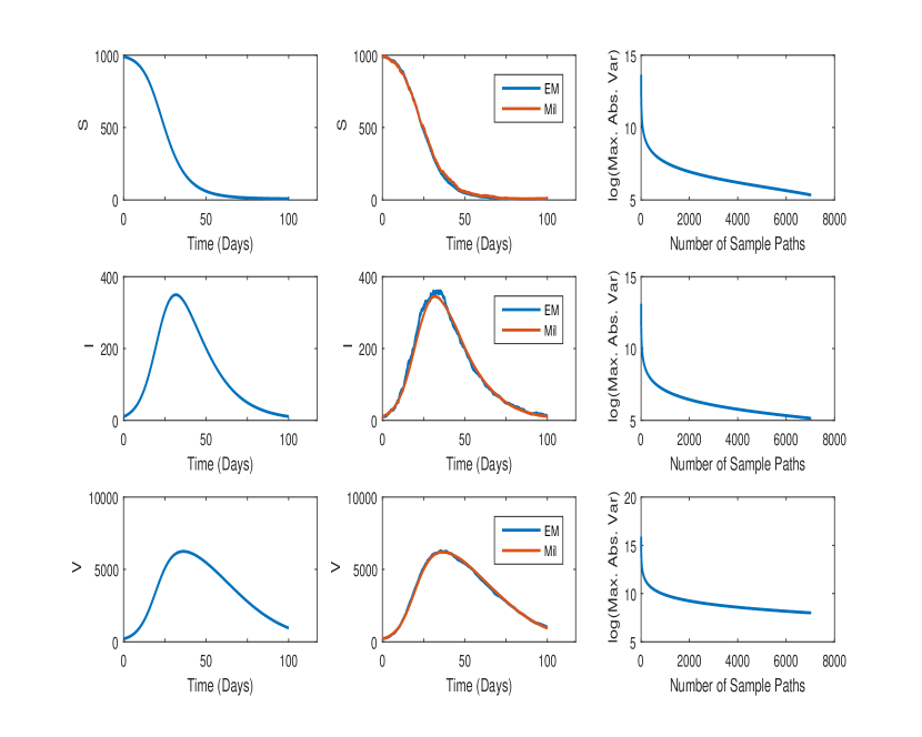
Figure 1: Solution to the model 1 and 2 when $n=1$. The reproduction number of the single patch model is $\mathbf{R}_{0}=3.1614$. The initial susceptible hosts, infected hosts and infected vectors used in the simulations are 990, 10 and 200 respectively. The total number of hosts and vectors are 1000 and 10000 respectively. Parameters used in the simulations are $\beta=1/7$, $\mu=1/(69\times 365)$, $\gamma=(1/14)$, $\nu=1/10$, and $\vartheta=5\nu$.

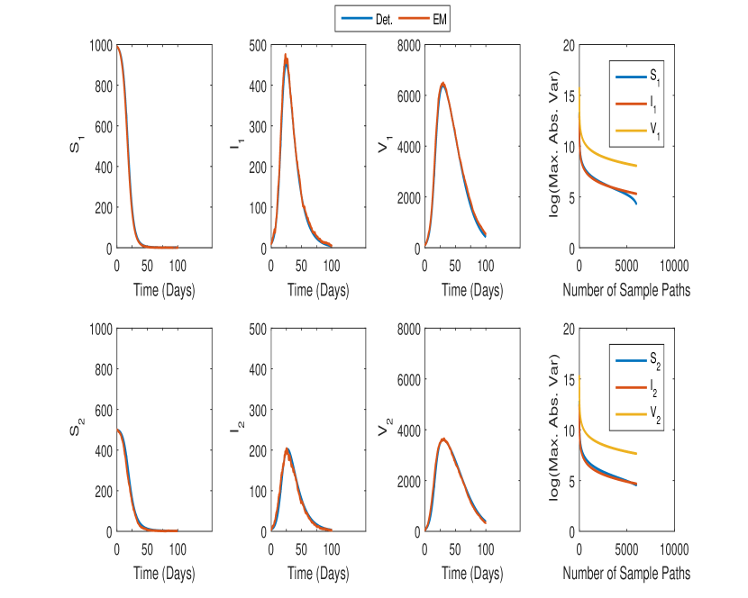
Figure 2: Solution to the model 1 and 2 in the case of $n=2$. The initial susceptible hosts, infected hosts and infected vectors used in the simulations are given in the order of ($S_{i},I_{i},V_{i}=(990,500,10,5,100,50)$) respectively. The total number of hosts and vectors are ($N_{i},M_{i}=(1000,500)$). Parameters used in the simulations are $\beta_{i}=(2/7,1/7)$, $\mu_{i}=1/(69\times 365)$, $\gamma_{i}=(1/14)$, $\nu_{i}=1/10$, and $\vartheta_{i}=5\nu_{i}$.

In Figure 1, subplots shown by the first column refers to the deterministic solutions of the three state variables for $S$, $I$, and $V$ with reference to the single patch model where, subplots in the second column presents the mean of the numerical solutions of 7000 realizations obtained by solving the SDE model by using the Euler-Maruyama and Milstein schemes. Subplots shown by the third column illustrates the logarithm of the maximum variance obtained via the numerical scheme Euler-Maruyama, against the number of sample paths. It is clearly visible from the subplots in the third column that when the number of sample paths are higher the maximum variance of the solution gets gradually decreased.

Figure 2, compares the mean solutions obtained via the Euler-Maruyama scheme to the stochastic model (2) with the deterministic solutions for the two-patch model. Similar to the single patch model here also, the logarithm of the maximum variance of the average solutions reduce over the increment of number of sample paths.

5 Discussion

It can be concluded by the results obtained for the single patch model (Figure: 1) that the solutions of the stochastic model is closely similar to the mean of the deterministic solution with a higher number of sample paths and further, it has been confirmed by the variance plot where it illustrates that when the number of sample paths increase the variance of the solutions gets close enough to zero. Also, the plot confirms that the solutions obtained via Milstein scheme gives more close results to the deterministic solution than the Euler-Maruyama scheme. The movement of the hosts within the areas highly impact on the disease spread and here, it is investigated that the SDE model is closely related with the ODE model giving close results to the deterministic solutions. In Figure: 2 the stochastic solutions are derived and compared with the deterministic solutions only via Euler-Maruyama scheme because there are some major difficulties in implementing the Milstein scheme to vector valued Wiener process, because the double stochastic integrals present in the scheme makes complexities with the implementation and will be of future interest to implement the two-patch model. The results, which are present in this paper are for $n=2$, for better understanding but without any problem the simulations can be performed to a more generalized system with $n$ patches.

References

- [1] Allen, L. J. S.: An introduction to stochastic processes with applications to biology (2003)
- [2] Bock, W. and Jayathunga, Y. : Optimal control and basic reproduction numbers for a compartmental spatial multipatch dengue model. Mathematical Methods in the Applied Sciences. 41(9), 3231–3245 (2018)
- [3] Götz,T. , Altmeier,N. , Bock, W., Rockenfeller, R., Sutimin, and Wijaya, K. P. : Ann. Mat. Pura. Appl. Modeling dengue data from semarang, indonesia (2016)
- [4] Gubler, D. J.: Dengue, urbanization and globalization: the unholy trinity of the 21st century. Tropical medicine and health. 39, S3–S11 (2011)
- [5] Lee, S. and Castillo-Chavez, C.: The role of residence times in two-patch dengue transmission dynamics and optimal strategies. Journal of theoretical biology. 374, 152–164 (2015)
- [6] Morlan, H. B. and Hayes, R. O. : Urban dispersal and activity of aedes aegypti. Mosq News. 18,137–144 (1958)
- [7] Muir, L. E. and Kay, B. H. : Aedes aegypti survival and dispersal estimated by mark-release-recapture in northern australia. The American Journal of Tropical Medicine and Hygiene. 58(3), 277–282 (1998)
- [8] Normile, D. : Surprising new dengue virus throws a spanner in disease control efforts. Science. 342(6157), 415–415 (2013)
- [9] Páez Chávez, J. , Götz, T., Siegmund, S. and Wijaya, K. P. : An SIR-Dengue transmission model with seasonal effects and impulsive control. Math. Biosci. 289, 29–39 (2017)
- [10] Rocha, F., Aguiar, M. and Stollenwerk, N. : The influence of the vector aedes aegypti in dynamics of the epidemiology of dengue fever.
- [11] Rodrigues, H. S., Teresa, M., Monteiro, T. and Torres, D. F. M.: Vaccination models and optimal control strategies to dengue. Math. Biosci. 247, 1–12 (2014)
- [12] United Nations.: World population prospects: The 2017 revision, key findings and advance tables. esa.un.org/ (2017)
- [13] Van den Driessche, P. and Watmough, J.: Reproduction numbers and sub-threshold endemic equilibria for compartmental models of disease transmission. Mathematical biosciences. 180(1), 29–48 (2002)
- [14] World Health Organization, in Dengue Prevention and Control (2016) http://iris.wpro.who.int/bitstream/handle/10665.1/13599/9789290618256-eng.pdf?ua=1