Abstract

Recent work has explored transforming data sets into smaller, approximate summaries in order to scale Bayesian inference. We examine a related problem in which the parameters of a Bayesian model are very large and expensive to store in memory, and propose more compact representations of parameter values that can be used during inference. We focus on a class of graphical models that we refer to as latent Dirichlet-Categorical models, and show how a combination of two sketching algorithms known as count-min sketch and approximate counters provide an efficient representation for them. We show that this sketch combination – which, despite having been used before in NLP applications, has not been previously analyzed – enjoys desirable properties. We prove that for this class of models, when the sketches are used during Markov Chain Monte Carlo inference, the equilibrium of sketched MCMC converges to that of the exact chain as sketch parameters are tuned to reduce the error rate.

1 Introduction

The development of scalable Bayesian inference techniques (Angelino et al., 2016) has been the subject of much recent work. A number of these techniques introduce some degree of approximation into inference.

This approximation may arise by altering the inference algorithm. For example, in “noisy” Metropolis Hastings algorithms, acceptance ratios are perturbed because the likelihood function is either simplified or evaluated on a random subset of data in each iteration (Negrea and Rosenthal, 2017; Alquier et al., 2014; Pillai and Smith, 2014; Bardenet et al., 2014). Similarly, asynchronous Gibbs sampling (Sa et al., 2016) violates some strict sequential dependencies in normal Gibbs sampling in order to avoid synchronization costs in the distributed or concurrent setting.

Other approaches transform the original large data set into a smaller representation, on which traditional inference algorithms can then be efficiently run. Huggins et al. (2016) compute a weighted subset of the original data, called a coreset. Geppert et al. (2017) consider Bayesian regression with $n$ data points each of dimension $d$, and apply a random projection to shrink the original $\mathbb{R}^{n\times d}$ data set down to $\mathbb{R}^{k\times d}$ for $k<n$. An advantage of these kinds of transformations is that by shrinking the size of the data, it becomes more feasible to fit the transformed data set entirely in memory.

The transformations described in the previous paragraph reduce the number of data points under consideration, but preserve the dimension of each data point, and thus the number of parameters in the model. However, in many Bayesian mixed membership models, the number of parameters themselves can also become extremely large when working with large data sets, and storing these parameters poses a barrier to scalability.

In this paper, we consider an approximation to address this issue for what we call latent Dirichlet-Categorical models, in which there are many latent categorical variables whose distributions are sampled from Dirichlets. This is a fairly general pattern that can be found as a basic building block of many Bayesian models used in NLP (e.g., clustering of discrete data, topic models like LDA, hidden Markov models). The most representative example, which we will use throughout this paper, is the following:

$$z_{i} \sim\tt Categorical(\tau) i\in[N]$$ (1)

$$\theta_{i} \sim\tt Dirichlet(\alpha) i\in[K]$$ (2)

$$x_{i} \sim\tt Categorical(\theta_{z_{i}}) i\in[N]$$ (3)

Here, $\tau$ is some fixed hyper-parameter of dimension $K$ and $\alpha$ is a scalar value. We assume that the dimension of the Dirichlet distribution is $V$, a value we refer to as the “vocabulary size”. Each random variable $x_{i}$ can take one of $V$ different values, which we refer to as “data types” (e.g., words in latent Dirichlet allocation).

To do Gibbs sampling for a model in which such a pattern occurs, we generally need to compute a certain matrix $c$ of dimension $K\times V$. Each row of this matrix tracks the frequency of occurrence of some data type within one of the components of the model. In general, this matrix can be quite large, and in some cases we may not even know the exact value of $V$ a priori (e.g., consider the streaming setting where we may encounter new words during inference), making it costly to store these counts. Moreover, if we do distributed inference by dividing the data into subsets, each compute node may need to store this entire large matrix, which reduces the amount of data each node can store in memory and adds communication overhead. Although $c$ is often sparse, using a sparse or dynamic representation instead of a fixed array makes updates and queries slower, and adds further overhead when merging distributed representations.

We propose to address these problems by using sketch algorithms to store compressed representations of these matrices. These algorithms give approximate answers to certain queries about data streams while using far less space than algorithms that give exact answers. For example, the count-min sketch (CM) (Cormode and Muthukrishnan, 2005) can be used to estimate the frequency of items in a data set without having to use space proportional to the number of distinct items, and approximate counters (Morris, 1978; Flajolet, 1985) can store very large counts with sublogarithmic number of bits. These algorithms have parameters that can be tuned to trade between estimation error and space usage. Because many natural language processing tasks involve computing estimates of say, the frequency of a word in a corpus, there has been obvious prior interest in using these sketching algorithms for (non-Bayesian) NLP when dealing with very large data sets (Durme and Lall, 2009b; Goyal and Daumé III, 2011; Durme and Lall, 2009a).

We propose representing the matrix $c$ above using a combination of count-min sketch and approximate counters. It is not clear a priori what effect this would have on the MCMC algorithm. On the one hand, it is plausible that if the sketch parameters are set so that estimation error is small enough, MCMC will still converge to some equilibrium distribution that is close to the equilibrium distribution of the exact non-sketched version. On the other hand, we might be concerned that even small estimation errors within each iteration of the sampler would compound, causing the equilibrium distribution to be very far from that of the non-sketched algorithm.

In this paper, we resolve these issues both theoretically and empirically. We prove results showing that under fairly general conditions, as the parameters of sketches are tuned to decrease the error rate, the equilibrium distributions of sketched chains converge to that of the exact chain. Then, we show that when the combined sketch is used with a highly scalable MCMC algorithm for LDA, we can obtain model quality comparable to that of the non-sketched version while using much less space.

Contribution

1. We explain how the count-min sketch algorithm and approximate counters can be used to sketch the sufficient statistics of models that contain latent Dirichlet-Categorical subgraphs (section §2). We then provide an analysis of a combined count-min sketch/approximate counter data structure which provides the benefits of both (section §3).

2. We then prove that when the combined sketch is used in an MCMC algorithm, as the parameters of the sketch are tuned to reduce error rates, the equilibrium distributions of sketched chains converge to that of the non-sketched version (section §4).

3. We complement these theoretical results with experimental evidence confirming that learning works despite approximations introduced by the sketches (section §5).

2 Sketching for Latent Dirichlet-Categorical Models

As described in the introduction, MCMC algorithms for models involving Dirichlet-Categorical distributions usually require tabulating statistics about the current assignments of items to categories (e.g., the words per topic in LDA). There are two reasons why maintaining this matrix of counts can be expensive. First, the dimensions of the matrix can be large – the dimensions are often proportional to the number of unique words in the corpus. Second, the values in the matrix can also be large, so that tracking them using small sized integers can potentially lead to overflow.

Sketching algorithms can be used to address these problems, providing compact fixed-size representations of these counts that use far less memory than a dense array. We start by explaining two widely used sketches, and then in the next section discuss how they can be combined.

2.1 Sketch 1: count-min sketch

To deal with the fact that the matrix of counts is of large dimension, we can use count-min (CM) sketches (Cormode and Muthukrishnan, 2005) instead of dense arrays. A CM sketch $\mathcal{C}$ of dimension $l\times w$ is represented as an $l\times w$ matrix of integers, initialized at 0, and supports two operations: update and query. The CM sketch makes use of $l$ different 2-universal hash functions of range $w$ that we denote by $h_{1},\dots,h_{l}$. The update$(x)$ operation adjusts the CM sketch to reflect an increment to the frequency of some value $x$, and is done by incrementing the matrix at locations $\mathcal{C}_{i,h_{i}(x)}$ for $i\in[1,l]$. The query($x$) operation returns an estimate of the frequency of value $x$ and is computed by $\min_{i}\mathcal{C}_{i,h_{i}(x)}$.

It is useful to think of a value $C_{a,b}$ in the matrix as a random variable. In general, when we study an arbitrary value, say $x$, we need not worry about where it is located in row $i$ and refer to $\mathcal{C}_{i,h_{i}(x)}$ simply as $Z_{i}$, and write $Q(x)\mathrel{:=}\min_{i}(Z_{i})$ for the result when querying $x$. Note that $Z_{i}$ equals the true number of occurrences of $x$, written $f_{x}$, plus the counts of other keys whose hashes are identical to that of $x$. CM sketches have several interesting properties, some of which we summarize here (see Roughgarden and Valiant (2015) for a good expository account). Let $N$ be the total number of increments to the CM sketch. Then, each $Z_{i}$ is a biased estimator, in that:

$$\mathbb{E}[Z_{i}]=f_{x}+\frac{N-f_{x}}{w}$$ (4)

However, by adjusting the parameters $l$ and $w$, we can bound the probability of large overestimation. In particular, by taking $w=\frac{k}{\epsilon}$ one can bound the offset of a query as

$$\Pr\left[Q(x)\geq f_{x}+\epsilon N\right]\leq\frac{1}{k^{l}}$$ (5)

A nice property of CM sketches is that they can be used in parallel: we can split a data stream up, derive a sketch for each piece, and then merge the sketches together simply by adding the entries in the different sketches together componentwise.

We want to replace the matrix of counts $c$ in a Dirichlet-Categorical model with sketches. There is some flexibility in how this is done. The simplest thing is to replace the entire matrix with a single sketch (so that the keys are the indices into the matrix). Alternatively, we can divide the matrix into sub-matrices, and use a sketch for each sub-matrix. In the setting of Dirichlet-Categorical models, each row of $c$ corresponds to the counts for data types within one component of the model (e.g., counts of words for a given topic in LDA), so it is natural to use a sketch per row.

2.2 Sketch 2: approximate counting

In order to represent large counts without the memory costs of using a large number of bytes, we can employ approximate counters (Morris, 1978). An approximate counter $X$ of base $b$ is represented by an integer (potentially only a few bits) initialized at 0, and supports two operations: increment and read. We write $X_{n}$ to denote a counter that has been incremented $n$ times. The increment operation is randomized and defined as:

$$\Pr(X_{n+1}=k+1\ |\ X_{n}=k)=b^{-k}$$ (6)

$$\Pr(X_{n+1}=k\ |\ X_{n}=k)=1-b^{-k}$$ (7)

Reading a counter $X$ is written as $\phi(X)$ and defined as $\phi(X)=(b^{X}-1)/(b-1)$. Approximate counters are unbiased, and their variance can be controlled by adjusting $b$:

$$\mathbb{E}[\phi(X_{n})]=n\qquad\mathbb{V}\left[\phi(X_{n})\right]=\frac{b-1}{2}(n^{2}-n)$$ (8)

Using approximate counters as part of inference for Dirichlet-Categorical models is very simple: instead of representing the matrix $c$ as an array of integers, we instead use an array of approximate counters.

3 Combined Sketching: Alternatives and Analysis

The problems addressed by the sketches described in the previous section are complementary: CM sketches replace a large matrix with a much smaller set of arrays; but by coalescing increments for distinct items, CM sketches need to potentially store larger counts to avoid overflows, a problem which is resolved with approximate counting. Therefore, it is natural to consider how to combine the two sketching algorithms together.

3.1 Combination 1: Independent Counters

The simplest way to combine the CM sketch with approximate counters is to replace each exact counter in the CM sketch with an approximate counter; then when incrementing a key in the sketch, we independently increment each of the counters it corresponds to. Moreover, because there are ways to efficiently add together two approximate counters (Steele and Tristan, 2016), we can similarly merge together multiple copies of these sketches by once again adding their entries together componentwise.

When we combine the CM sketch and the approximate counters together in this way, the errors introduced by these two kinds of algorithms interact. It is challenging to give a precise analysis of the error rate of the combined structure. However, it is still the case that we can tweak the parameters of the sketch to make the error rate arbitrarily low.

To make this precise, note that we now have three parameters to tune: $b$, the base of the approximate counters, $l$ the number of hashes, and $w$, the range of the hashes. Given a parameter triple $\psi=(b,l,w)$, write $Q_{\psi}(x)$ for the estimate of key $x$ from a sketch using these parameters. Then, given a sequence $\psi_{n}=(b_{n},l_{n},w_{n})$ of parameters, we can ask what happens to the sequence of estimates $Q_{\psi_{n}}(x)$ when we use the sketches on the same fixed data set:

Theorem 3.1.

Let $\psi_{n}=(b_{n},l_{n},w_{n})$. Suppose $b_{n}\rightarrow 1$, $w_{n}\to\infty$ and there exists some $L$ such that $1\leq l_{n}\leq L$ for all $n$. Then for all $x$, $Q_{\psi_{n}}(x)$ converges in probability to $f_{x}$ as $n\to\infty$.

See Appendix A in the supplementary material for the full proof. This result shows that for appropriate sequences $\psi_{n}$ of parameters, the estimator $Q_{\psi_{n}}(x)$ is consistent. We call a sequence $\psi_{n}$ satisfying the conditions of Theorem 3.1 a consistent sequence of parameters.

For our application, we are replacing a matrix of counts with a collection of sketches for each row, so we want to know not just about the behavior of the estimate of a single key in one of these sketches, but about the estimates for all keys across all sketches. Formally, let $c$ be a $K\times V$ dimensional matrix of counts. Consider a collection of $K$ sketches, each with parameters $\psi$, where for each key $v$, we insert $v$ with frequency $c_{k,v}$ into the $k$th sketch. then we write $Q_{\psi}(c)$ for the random $K\times V$ matrix giving the estimates of all the keys in each sketch. Because convergence in probability of a random vector follows from convergence of each of the components, the above implies:

Theorem 3.2.

If $\psi_{n}$ is a consistent sequence, then $Q_{\psi_{n}}(c)$ converges in probability to $c$.

Finally, we have been describing the situation where the keys are inserted with some deterministic frequency and the only source of randomness is in the hashing of the keys and the increments of the approximate counter. However, it is natural to consider the case where the frequency of the keys is randomized as well. To do so, we define the Markov kernel $T_{\psi}$ from $\mathbb{N}^{K\times V}$ to $\mathbb{R}_{\geq 0}^{K\times V}$, where for each $c$, $T_{\psi}(c,\cdot)$ is the distribution of the random variable $Q_{\psi}(c)$ considered above. Then if $\mu$ is a distribution on count matrices, $\mu T_{\psi}$ gives the distribution of query estimates returned for the sketched matrix.

3.2 Combination 2: Correlated Counters

Even though the results above show that the approximation error of the combined sketch can still be made arbitrarily small, it does not provide a non-asymptotic bound on the error. Indeed, one issue with this combination is that the traditional estimation rule for the sketch relies on the fact that for a key $x$, each of the cells $Z_{1},\dots,Z_{l}$ corresponding to $x$ is at least as large as $f_{x}$, the true frequency of $x$. Therefore, the minimum is the closest estimate of the count. But when we instead use approximate counters, it is possible for each counter’s estimate to be smaller than $f_{x}$, so taking the minimum may cause underestimation.

This underestimation rules out using the so-called conservative update rule (Estan and Varghese, 2002), a technique which can be used to reduce bias of normal CM sketches. When using conservative update with a regular CM sketch, to increment a key $x$, instead of incrementing each of the counters corresponding to $x$, we first find the minimum value and then only increment counters equal to this minimum. But because approximate counters can underestimate, this is no longer justifiable in the combined sketch.

Pitel and Fouquier (2015) proposed an alternative way to combine CM sketches with approximate counters that enables conservative updates. We call their combination correlated counters. Figure 1 shows the increment routine with and without conservative update for correlated counters. The idea in each is that we generate a single uniform $[0,1]$ random variable $r$ and use this common $r$ to decide how to transition each counter value according to the probabilities described in §2.2.

1:procedure incr-correlated($C$, $x$)

2:   let $r$ $\leftarrow$ Uniform(0, 1)

3:   for $i$ from 0 to $l$ do

4:      let $v$ $\leftarrow$ $C$[$i$][$h_{i}(x)$]

5:      if $r<\frac{1}{b^{v}}$ then $C$[$i$][$h_{i}(x)$] $\leftarrow$ $v+1$

6:   end for

7:

8:procedure incr-conservative($C$, $x$)

9:   let $r$ $\leftarrow$ Uniform(0, 1)

10:   let $min$ $\leftarrow$ $\infty$

11:   for $i$ from 0 to $l$ do

12:      let $v$ $\leftarrow$ $C$[$i$][$h_{i}(x)$]

13:      if $v<min$ then $min$ $\leftarrow$ $v$

14:   end for

15:

16:   if $r<\frac{1}{b^{min}}$ then

17:      for $i$ from 0 to $l$ do

18:         if $C[i][h_{i}(x)]=min$ then

19:            $C[i][h_{i}(x)]$ $\leftarrow$ $min+1$          

20:      end for   

21:

Figure 1: Increment for CM sketch with correlated approximate counters, with and without conservative update.

However, Pitel and Fouquier (2015) did not give a proof of any statistical properties of their combination. The following result shows that this variant avoids the underapproximation bias of the independent counter version:

Theorem 3.3.

Let $Q(x)$ be the query result for key $x$ using correlated counters in a CM sketch with one of the increment procedures from Figure 1. Then,

$$f_{x}\leq\mathbb{E}[Q(x)]\leq f_{x}+\frac{N-f_{x}}{w}$$

Proof 1.

We discuss just the non-conservative update increment procedure, since the proof is similar for the other case. The upper bound is straightforward. The lower bound is proved by exhibiting a coupling (Lindvall, 2002) between the sketch counters corresponding to key $x$ and a counter $C$ of base $b$ that will be incremented exactly $f_{x}$ times. The coupling is constructed by induction on $N$, the total number of increments to the sketch. Throughout, we maintain the invariant that $\phi(C)\leq Q(x)$; it follows that $\mathbb{E}[\phi(C)]\leq\mathbb{E}[Q(x)]$. Since $\mathbb{E}[\phi(C)]=f_{x}$, this will give the desired bound.

In the base case, when $N=0$, both $\phi(C)$ and $Q(x)$ are $0$ so the invariant holds trivially. Suppose the invariant holds after the first $k$ increments to the sketch, and some key $y$ is then incremented. If $x=y$, then we transition the counter $C$ using the same random uniform variable $r$ that is used to transition the counters $X_{1},\dots,X_{l}$ corresponding to key $x$ in the sketch. There are two cases: either $r$ is small enough to cause the minimum $X_{i}$ to increase by 1, or not. If it is, then since $C\leq\min_{i}(X_{i})$, $r$ is also small enough to cause $C$ to increase by 1, and so $\phi(C)\leq Q(x)$. If $\min_{i}(X_{i})$ does not change, but $C$ does, then we must have $C<\min_{i}(X_{i})$ before the transition; since $C$ can only increase by $1$, we still have $C\leq\min_{i}(X_{i})$ afterward.

If the key $y$ is not equal to $x$, then we leave $C$ as is. Since the $X_{i}$ can only possibly increase while $C$ stays the same, the invariant holds. Finally, after all $N$ increments have been performed, $C$ will have received $f_{x}$ increments, so that $\mathbb{E}[\phi(C)]=f_{x}$ because approximate counters are unbiased.

In Appendix D we describe various microbenchmarks comparing the behavior of the different ways of combining the two sketches.

4 Asymptotic Convergence

In the previous section, we explored some of the statistical properties of the combined sketch. We now turn to the question of the behavior of an MCMC algorithm when we use these sketches in place of exact counts. More precisely, suppose we have a Markov chain whose states are tuples of the form $(c,z)$, where $c$ is a $K\times V$ matrix of counts, and $z$ is an element of some complete separable metric space $Y$. Now, suppose instead of tabulating $c$ in a dense array of exact counters, we replace each row with a sketch using parameters $\psi$. We can ask whether the resulting sketched chain has an equilibrium distribution, and if so, how it relates to the equilibrium distribution of the original “exact” chain. As we will see, it is often easy to show that the sketched chain still has an equilibrium distribution. However, the relationship between the sketched and exact equilibriums may be quite complicated. Still, a reasonable property to want is that, if we have a consistent sequence of parameters $\psi_{n}$, and we consider a sequence of sketched chains, where the $i$th chain uses parameters $\psi_{i}$, then the sequence of equilibrium distributions will converge to that of the exact chain.

The reason such a property is important is that it provides some justification for how these sketched approximations would be used in practice. Most likely, one would first test the algorithm using some set of sketch parameters, and then if the results are not satisfactory, the parameters could be adjusted to decrease error rates in exchange for higher computational cost. (Just as, when using standard MCMC techniques without an a priori bound on mixing times, one can run chains for longer periods of time if various diagnostics suggest poor results). Therefore, we would like to know that asymptotically this approach really would converge to the behavior of the exact chain. We will now show that under reasonable conditions, this convergence does in fact hold.

We assume the state space $S_{\textsf{e}}$ of the original chain is a compact, measurable subset of $\mathbb{N}^{K\times V}\times Y$. We suppose that the transition kernel of the chain can be divided into three phrases, represented by the composition of kernels $K_{\textsf{pre}}\cdot K\cdot K_{\textsf{post}}$, where in $K$ the matrix of counts is updated in a way that depends only on the rest of the state, which is then modified in $K_{\textsf{pre}}$ and $K_{\textsf{post}}$ (e.g., in a blocked Gibbs sampler $K$ would correspond to the part of a sweep where $c$ is updated). Moreover, we assume that the transitions $K_{\textsf{pre}}$ and $K_{\textsf{post}}$ are well-defined on the extended state space $\mathbb{R}_{\geq 0}^{K\times V}\times Y$, where the counts are replaced with positive reals. Formally, these conditions mean we assume that there exist Markov kernels $K_{\textsf{pre}}^{\prime},K_{\textsf{post}}^{\prime}:\mathbb{R}_{\geq 0}^{K\times V}\times Y\rightarrow Y$ and $K:Y\rightarrow\mathbb{N}^{K\times V}$ such that

$$K_{\textsf{pre}}((c,z),A) =\int K_{\textsf{pre}}^{\prime}((c,z),dz^{\prime})1_{A}(c,z^{\prime})$$

$$K((c,z),A) =\int K^{\prime}(z,dc^{\prime})1_{A}(c^{\prime},z)$$

$$K_{\textsf{post}}((c,z),A) =\int K_{\textsf{post}}^{\prime}((c,z),dz^{\prime})1_{A}(c,z^{\prime})$$

where we write $1_{A}$ for the indicator function corresponding to a measurable set $A$. We assume this chain has a unique stationary distribution $\mu$. Furthermore, we assume $K_{\textsf{pre}}$, $K$, and $K_{\textsf{post}}$ are Feller continuous, that is, if $s_{n}\rightarrow s$, then $K(s_{n},\cdot)\Rightarrow K(s,\cdot)$, and similarly for $K_{\textsf{pre}}$ and $K_{\textsf{post}}$, where $\Rightarrow$ is weak convergence of measures.

Fix a consistent sequence of parameters $\psi_{n}$. For each $n$, we define the sketched Markov chain with transition kernel $K_{\textsf{pre}}\cdot K_{n}\cdot K_{\textsf{post}}$, where $K_{n}$ is the kernel obtained by replacing the exact matrix of counts used in $K$ with a sketched matrix with parameters $\psi_{n}$:

$$K_{n}((c,z),A)$$

$$=\int K^{\prime}(z,dc^{\prime})\int T_{\psi_{n}}(c^{\prime},dc^{\prime\prime})1_{A}(c^{\prime\prime},z)$$

(recall that $T_{\psi_{n}}$ is the kernel induced by the combined sketching algorithm, as described in §3.1). We assume that the set $S$ containing the union of the states of the exact chain and the sketched chains is some compact measurable subset of $\mathbb{R}_{\geq 0}^{K\times V}\times Y$. Assuming that each $K_{\textsf{pre}}\cdot K_{n}\cdot K_{\textsf{post}}$ has a stationary distribution $\mu_{n}$, we will show that they converge weakly to $\mu$. We use the following general result of Karr:

Theorem 4.1 (Karr (1975, Theorems 4 and 6)).

Let $E$ be a complete separable metric space with Borel sigma algebra $\Sigma$. Let $K$ and $K_{1},K_{2},\dots$ be Markov kernels on $(E,\Sigma)$. Suppose $K$ has a unique stationary distribution $\mu$ and $K_{1},\dots$ have stationary distributions $\mu_{1},\dots$.
Assume the following hold

1. for all $s$, $\{K_{n}(s,\cdot)\}_{n}$ is tight, and

2. $s_{n}\rightarrow s$ implies $K_{n}(s_{n},\cdot)\Rightarrow K(s,\cdot)$.

Then $\mu_{n}\Rightarrow\mu$.

We now show that the assumptions of this theorem hold for our chains. The first condition is straightforward:

Lemma 4.2.

For all $x$, the family of measures $\{(K_{\textsf{pre}}\cdot K_{n}\cdot K_{\textsf{post}})(x,\cdot)\}_{n}$ is tight.

Proof 2.

This follows immediately from the assumption that the set of states $S$ is a compact measurable set.

To establish the second condition, we start with the following:

Lemma 4.3.

If $s_{n}\rightarrow s$, then $(K_{\textsf{pre}}\cdot K_{n})(s_{n},\cdot)\Rightarrow(K_{\textsf{pre}}\cdot K)(s,\cdot)$.

Proof 3.

To match up with the results in §3, it is helpful to rephrase this as a question of convergence of distribution of random variables with appropriate laws. By assumption $K_{\textsf{pre}}\cdot K$ is Feller continuous, so we know that $(K_{\textsf{pre}}\cdot K)(s_{n},\cdot)\Rightarrow(K_{\textsf{pre}}\cdot K)(s,\cdot)$, hence by Skorokhod’s representation theorem, there exists random matrices $C,C_{1},\dots,$ and random $Y$-elements $Z,Z_{1},\dots$ such that the law of $(C_{n},Z_{n})$ is $(K_{\textsf{pre}}\cdot K)(s_{n},\cdot)$, that of $(C,Z)$ is $(K_{\textsf{pre}}\cdot K)(s,\cdot)$, and $(C_{n},Z_{n})\xrightarrow[]{\textsf{p}}(C,Z)$. Then the distribution of $(Q_{\psi_{n}}(C_{n}),Z_{n})$ is that of $(K_{\textsf{pre}}\cdot K_{n})(s_{n},\cdot)$, so it suffices to show that $Q_{\psi_{n}}(C_{n})\xrightarrow[]{\textsf{p}}C$.

Fix $\delta,\epsilon>0$. Let $U$ be the union of the supports of each $C_{n}$. Then $U$ consists of integer matrices lying in some compact subset of real vectors (since $S$ is compact and the counts returned by $K$ are exact integers), so $U$ is finite. Moreover, by Theorem 3.2 we know that for all $c$, there exists $n_{c}$ such that for all $n>n_{c}$, $\Pr\left[\lVert Q_{\psi_{n}}(C_{n})-c\rVert>\epsilon/2\ \mid\ C_{n}=c\right]<\delta/2$. Let $m_{1}$ be the maximum of the $n_{c}$ for $c\in U$. We also know that there exists $m_{2}$ such that for all $n>m_{2}$, $\Pr\left[\lVert C_{n}-C\rVert>\epsilon/2\right]<\delta/2$. For $n>\max(m_{1},m_{2})$, we then have $\Pr\left[\lVert Q_{\psi_{n}}(C_{n})-C\rVert>\epsilon\right]<\delta$.

Continuity of $K_{\textsf{post}}$ then gives us:

Lemma 4.4.

If $s_{n}\rightarrow s$, then $(K_{\textsf{pre}}\cdot K_{n}\cdot K_{\textsf{post}})(s_{n},\cdot)\Rightarrow(K_{\textsf{pre}}\cdot K\cdot K_{\textsf{post}})(s,\cdot)$.

Thus by Karr’s theorem we conclude:

Theorem 4.5.

$\mu_{n}\Rightarrow\mu$.

In the above, we have assumed that there is a single sketched matrix of counts, and that each row of the matrix uses the same sketch parameters. However, the argument can be generalized to the case where there are several sketched matrices with different parameters. We now explain how this result can be applied to some Dirichlet-Categorical models:

Example 1: SEM for LDA.

When using stochastic expectation maximization (SEM) for the LDA topic model (Blei et al., 2003), the states of the Markov chain are matrices $wpt$ and $tpd$ giving the words per topic and topic per document counts. Within each round, estimates of the corresponding topic and document distributions $\theta$ and $\phi$ are computed from smoothed versions of these counts; new topic assignments are sampled according to this distribution, and the counts $wpt$ and $tpd$ are updated. We can replace the rows of either $wpt$ or $tpd$ with sketches. In this case $K_{\textsf{pre}}$ and $K_{\textsf{post}}$ are the identity, and the Feller continuity of $K$ follows from the fact that the estimates of $\theta$ and $\phi$ are continuous functions of the $\mathit{wpt}$ and $\mathit{tpd}$ counts. Compactness of the state space is a consequence of the fact that the set of documents (and hence maximum counts) are finite, and the maximum counter base is bounded. Finally, the sketched kernels still have unique stationary distributions because the smoothing of the $\theta$ and $\phi$ estimates guarantees that if a state is representable in the sketched chain, we can transition to it in a single step from any other state.

Example 2: Gibbs for Pachinko Allocation.

The Pachinko Allocation Model (PAM) (Li and McCallum, 2006) is a generalization of LDA in which there is a hierarchy of topics with a directed acyclic structure connecting them. A blocked Gibbs sampler for this model can be implemented by first conditioning on topic distributions and sampling topic assignments for words, then conditioning on these topic assignments to update topic distributions – in the latter phase, one needs counts of the occurrences of words in the different topics and subtopics which can be collected using sketches. Since the priors for sampling topics based on these counts are smoothed, the sketched chains once again have unique stationary distributions for the same reason as in LDA.

5 Experimental Evaluation

We now examine the empirical performance of using these sketches. We implemented a sketched version of SCA (Zaheer et al., 2016), an optimized form of SEM which is used in state of the art scalable topic models (Zaheer et al., 2016; Zhao et al., 2015; Chen et al., 2016; Li et al., 2017), and apply it LDA. Full details of SCA can be found in the appendix.

Setup

We fit LDA (100 topics, $\alpha=0.1$, $\beta=0.1$, 291k-word vocabulary after removing rare and stop-words as is customary) to 6.7 million English Wikipedia articles using 60 iterations of SCA distributed across eight 8-core machines, and measure the perplexity of the model after each iteration on 10k randomly sampled Reuters documents. For all experiments, we report the mean and standard-deviation of perplexity and timing across three trials. Example topics from the various configurations are shown in the appendix. For more details, see Appendix C.1.

In this distributed setting, each machine must store a copy of the word-per-topic ($wpt$) frequency counts, and at the end of an iteration, updated counts from different machines must be merged. However, each machine only needs to store the rows of the topics-per-document matrix ($tpd$) pertaining to the documents it is processing. Hence, controlling the size of $wpt$ is more important from a scalability perspective, so we will examine the effects of sketching $wpt$.

The data set and number of topics we are using for these tests are small enough that the non-sketched $wpt$ matrix and documents can feasibly fit in each machine’s memory, so sketching is not strictly necessary in this setting. Our reason for using this data set is to be able to produce baselines of statistical performance for the non-sketched version to compare against the sketched versions.

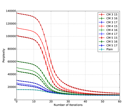
Figure 2: LDA perplexity with count-min sketch.

Experiment 1: Impact of the CM sketch.

In the first experiment, we evaluate the results of just using the CM sketch. We replace each row of the $wpt$ matrix in baseline plain SCA with a count-min sketch. We vary the number of hash functions $l\in\{3,4,5\}$ and the bits per hash from $\{15,16,17\}$. Figure 2 displays perplexity results for these configurations. While the more compressive variants of the sketches start at worse perplexities, by the final iterations, they converge to similar perplexities as the exact baseline with arrays. The range of the hash has a much larger effect than the number of hash functions in the earlier iterations of inference.

Table 1 gives timing and space usage (the first row corresponds to the baseline time and space). Recall that our main interest in sketching is to reduce space usage. Note that some of the parameter configurations here use more space than a dense array, so the purpose of including them is to better understand the statistical and timing effects of the parameters. Even though the smaller configurations do save space compared to the baseline, hashing the keys adds time overheads. Again, this is relative to the ideal case for the baseline, in which the documents and the full $wpt$ matrix represented as a dense array can fit in main memory.

$l$	$\log_{2}(w)$	time (s)	size ($10^{5}$ bytes)
NA	NA	12.14 $\pm$ 1.82	1164.0
3	15	22.75 $\pm$ 4.30	393.2
3	16	23.90 $\pm$ 4.41	786.43
3	17	25.32 $\pm$ 4.68	1572.9
4	15	29.70 $\pm$ 5.82	524.3
4	16	32.75 $\pm$ 6.17	1048.6
4	17	33.35 $\pm$ 5.89	2097.2
5	15	37.76 $\pm$ 6.95	655.4
5	16	39.71 $\pm$ 7.01	1310.7
5	17	42.33 $\pm$ 7.75	2621.4

Table 1: Time per iteration and size of $wpt$ representation for LDA with CM sketch. The first row gives non-sketched baseline. 4-byte integers are used to store entries in the dense matrix and sketches.

Experiment 2: Combined Sketches

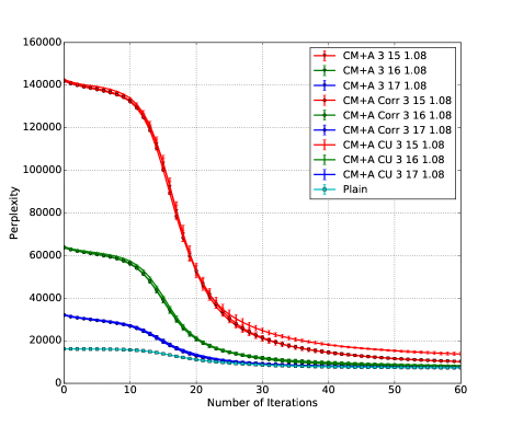
Figure 3: LDA perplexity with combined sketches.

For the next experiment (Figure 3), we use the three variants of combined sketches with approximate counters described in Section 3 (sketch with independent counters (CM+A), sketch with correlated counters (CM+A Corr), and sketch with correlated counters and the conservative update rule (CM+A CU)). We use 1-byte base-1.08 approximate counters in order to represent a similar range as a 4-byte integer (but using 1/4 the memory). Given the results of the previous experiment, we just consider the case where $3$ hash functions are used. In this particular benchmark, we do not see a large difference in perplexity between the various update rules, which again converge reasonably close to the perplexity of the baseline.

Table 2 gives timing and space usage for the combined sketches using the independent counter update rule. Each iteration runs faster than when just using the CM sketch with similar parameters. This is because the combined sketches are a quarter of the size of the CM sketch, so there is less communication complexity involved in sending the representation to other machines.

$l$	$\log_{2}(w)$	time (s)	size ($10^{5}$ bytes)
NA	NA	12.14 $\pm$ 1.82	1164.0
3	15	12.58 $\pm$ 2.00	98.3
3	16	17.57 $\pm$ 2.78	196.6
3	17	22.69 $\pm$ 3.72	393.22

Table 2: Time per iteration results for LDA with combined sketch using 1-byte, base 1.08 independent independent counters. Timing for other update rules are similar.

We explore a more comprehensive set of sketch and counter parameter effects on perplexity in Appendix E.3, run time in Appendix E.2, and example topics in Appendix E.1.

6 Conclusion

As machine learning models grow in complexity and datasets grow in size, it is becoming more and more common to use sketching algorithms to represent the data structures of learning algorithms. When used with MCMC algorithms, a primary question is what effect sketching will have on equilibrium distributions. In this paper we analyzed sketching algorithms that are commonly used to scale non-Bayesian NLP applications and proved that their use in various MCMC algorithms is justified by showing that sketch parameters can be tuned to reduce the distance between sketched and exact equilibrium distributions.

Appendix A Consistency of CM sketch with Approximate Counters

In this section, we prove Theorem 3.1 from §3.1:

Theorem 3.1.

Let $\psi_{n}=(b_{n},l_{n},w_{n})$. Suppose $b_{n}\rightarrow 1$, $w_{n}\to\infty$ and there exists some $L$ such that $l_{n}\leq L$ for all $n$. Let $Q_{\psi_{n}}$ be a sketch with these parameters, using either independent counters or correlated counters. Then for all $x$, $Q_{\psi_{n}}(x)$ converges in probability to $f_{x}$ as $n\to\infty$.

Proof 4.

Let $N$ be the sum of the frequencies of all keys. Fix some key $x$, and write $f_{x}$ for its true frequency. Now, for all $\delta,\epsilon>0$ we must show that there exists $n_{0}$ such that for $n^{\prime}>n_{0}$, $\Pr\left[|Q_{\psi_{n^{\prime}}}(x)-f_{x}|>\epsilon\right]<\delta$. Let $X_{n,i}$ be the random variable for the $i$th counter for key $x$ in sketch $n$, and let $Z_{n,i}$ be the random variable indicating how many times this counter is incremented.

As in the regular analysis of the count-min sketch, we have that $\mathbb{E}[Z_{n,i}]\leq f_{x}+\frac{N}{w_{n}}$ and $Z_{n,i}-f_{x}\geq 0$. Thus by Markov’s inequality applied to this difference, we have that $\Pr\left[Z_{n,i}-f_{x}>1/2\right]\leq\frac{2N}{w_{n}}$. Thus for large enough $w_{n}$, we can make this probability arbitrarily small. Since $w_{n}\rightarrow\infty$, there exists $n_{1}$ such that for $n>n_{1}$, $\Pr\left[Z_{n,i}-f_{x}>1/2\right]<\frac{\delta}{2L}$. Since $Z_{n,i}$ and $f_{x}$ are both integers, this implies $\Pr\left[Z_{n,i}\neq f_{x}\right]<\frac{\delta}{2L}$. Now, applying the Chebyshev bound to $X_{n,i}$ we have:

$$\Pr\left[|X_{n,i}-f_{x}|>\epsilon\mid Z_{n,i}=f_{x}\right]\leq\frac{b_{n}-1}{2\epsilon^{2}}(f_{x}^{2}-f_{x})$$

So that once more, for $b_{n}$ close enough to $1$, this probability will be less than $\frac{\delta}{2L}$, and there exists some $n_{2}$ such that for all $n>n_{2}$, $b_{n}$ will be sufficiently close to $1$. Set $n_{0}=\max(n_{1},n_{2})$, then we have that for $n>n_{0}$:

$$\Pr\left[|X_{n,i}-f_{x}|>\epsilon\right]$$

$$\quad=\Pr\left[|X_{n,i}-f_{x}|>\epsilon\mid Z_{n,i}=f_{x}\right]\Pr\left[Z_{n,i}=f_{x}\right]$$

$$\quad\qquad{}+\Pr\left[|X_{n,i}-f_{x}|>\epsilon\mid Z_{n,i}\neq f_{x}\right]\Pr\left[Z_{n,i}\neq f_{x}\right]$$

$$\quad\leq\frac{\delta}{L}$$

Thus we have that for such $n$:

$$\Pr\left[|Q_{\psi_{n}}(x)-f_{x}|>\epsilon\right] =\Pr\left[|\min_{i}X_{n,i}-f_{x}|>\epsilon\right]$$

$$\leq\sum_{i}^{l_{n}}\Pr\left[|X_{n,i}-f_{x}|>\epsilon\right]$$

$$\leq l_{n}\cdot\frac{\delta}{L}$$

$$\leq\delta$$

where the second inequality follows from the union bound. Because we use the union bound, it does not matter whether the $X_{n,i}$ are correlated for different $i$.

The above argument can be adapted to handle the case when we add together a finite number of sketches using the Steele and Tristan (2016) rule for adding approximate counters. The idea is to argue that when the base of the counters of the two summands are close to 1, they will both with high probability be equal to the “true” number of increments that have been performed to each, and similarly so will the sum.

Appendix B Bias from Merging Combined Sketches

As we have explained in the body of the paper, merging the combined sketches can be done using the addition routine of Steele and Tristan (2016). However, if these additions are done independently, this introduces potential for underestimation even in the case where correlated counters are used for incrementing within each sketch prior to merging. In this section we bound the resulting bias.

The expected values of maxima and minima of IID random variables is well studied. In particular, we have:

Theorem B.1 (Gumbel (1954), Hartley and David (1954)).

Let $Y_{1},\dots,Y_{l}$ be a collection of iid random variables, such that $\mathbb{E}[Y_{1}]=\mu$ and $\mathbb{V}\left[Y_{1}\right]=\sigma^{2}$.

$$\mathbb{E}[\max_{i}Y_{i}]\leq\mu+\sigma\left(\frac{l-1}{\sqrt{2l-1}}\right)$$

Let $X^{\prime}_{n}$ be the value of an approximate counter obtained by adding together several independent base $b$ counters that have been incremented a total of $n$ times collectively.

Then, the results of Steele and Tristan (2016) show that:

$$\mathbb{V}\left[\phi(X^{\prime}_{n})\right]\leq\frac{b-1}{2}(n^{2}-n)+\frac{1}{-2(b^{2}-4b+1)}$$

Note that this bound holds regardless of how many counters were added together or what their relative sizes were.

As Steele and Tristan (2016) point out, for $1<b\leq 2$, the right summand is less than $\frac{1}{4}$. Define $\xi(n)=\sqrt{\frac{b-1}{2}(n^{2}-n)}+\frac{1}{2}$, then we have that $\sqrt{\mathbb{V}\left[\phi(X^{\prime}_{n})\right]}\leq\xi(n)$ for $b$ in this range.

B.1 Merging Independent Counter Sketches

Let $Y^{\prime}_{1},\dots,Y^{\prime}_{l}$ be IID random variables such that each $Y^{\prime}_{i}$ is an approximate counter whose value is obtained by adding together several independent base $b$ counters that have been incremented a total of $n$ times collectively. Let $M^{\prime}_{b,l}(n)$ be $\min_{i}\phi(Y^{\prime}_{i})$.

Theorem B.2.

If $1<b\leq 2$, then

$$\mathbb{E}[M^{\prime}_{b,l}(n)]\geq n\left(1-\left(\sqrt{\frac{b-1}{2}}+\frac{1}{2n}\right)\left(\frac{l-1}{\sqrt{2l-1}}\right)\right)$$

Proof 5.

Applying Theorem B.1, we obtain:

$$\mathbb{E}[M^{\prime}_{b,l}(n)]$$

$$\geq n-\xi(n)\left(\frac{l-1}{\sqrt{2l-1}}\right)$$

$$\geq n\left(1-\left(\sqrt{\frac{b-1}{2}\left(1-\frac{1}{n}\right)}+\frac{1}{2n}\right)\left(\frac{l-1}{\sqrt{2l-1}}\right)\right)$$

$$\geq n\left(1-\left(\sqrt{\frac{b-1}{2}}+\frac{1}{2n}\right)\left(\frac{l-1}{\sqrt{2l-1}}\right)\right)$$

Then, if $Q$ is a CM sketch obtained by merging several sketches using independent counters, and $f_{x}$ is the total frequency of key $x$ across the sketches, then $\mathbb{E}[M^{\prime}_{b,l}(f_{x})]\leq\mathbb{E}[Q(x)]$

B.2 Merging Correlated Counter Sketches

If we use the correlated increment rule of Pitel and Fouquier (2015), then the counters corresponding to a key within each sketch are not independent, hence they are not independent in the merged sketch either, so the results of Theorem B.1 do not immediately apply. However, we can still obtain the same bound as in the independent case, as we will see.

To simplify the notation, we will just assume we are merging only two sketches; the proof generalizes to merging an arbitrary number of sketches. Let $f_{x,1}$ be the frequency that $x$ occurs in the data stream processed by the first sketch, and let $f_{x,2}$ be the frequency in the second sketch, so that $f_{x}=f_{x,1}+f_{x,2}$. Since we seek a lower bound $\mathbb{E}[Q(x)]$, and hash collisions between $x$ and other keys only possibly increase $\mathbb{E}[Q(x)]$, it suffices to bound the case when there are no collisions.

In that case, the correlated increment rule is the same whether we do conservative update or not, and the values of the counters for key $x$ within sketch $1$ are all equal, and similarly for all the counters within sketch $2$. Let $Y_{1}$ and $Y_{2}$ denote these values. For each $m$ and $n$, if we condition on $Y_{1}=m$ and $Y_{2}=n$, then the results of adding the cells for key $x$ are IID, and so Theorem B.1 applies once more, so that we get:

$$\mathbb{E}\left[Q(x)\ |\ Y_{1}=m,Y_{2}=n\right]$$ (9)

$$\geq(n+m)-\xi(n+m)\left(\frac{l-1}{\sqrt{2l-1}}\right)$$ (10)

$$\geq(n+m)\left(1-\sqrt{\frac{b-1}{2}}\left(\frac{l-1}{\sqrt{2l-1}}\right)\right)$$ (11)

$$\quad-\frac{1}{2}\left(\frac{l-1}{\sqrt{2l-1}}\right)$$ (12)

By the law of the total expectation, it follows that

$$\mathbb{E}[Q(x)]$$ (13)

$$\geq(\mathbb{E}[Y_{1}]+\mathbb{E}[Y_{2}])\left(1-\sqrt{\frac{b-1}{2}}\left(\frac{l-1}{\sqrt{2l-1}}\right)\right)$$ (14)

$$\quad-\frac{1}{2}\left(\frac{l-1}{\sqrt{2l-1}}\right)$$ (15)

$$=f_{x}\left(1-\sqrt{\frac{b-1}{2}}\left(\frac{l-1}{\sqrt{2l-1}}\right)\right)$$ (16)

$$\quad-\frac{1}{2}\left(\frac{l-1}{\sqrt{2l-1}}\right)$$ (17)

$$=f_{x}\left(1-\left(\sqrt{\frac{b-1}{2}}+\frac{1}{2f_{x}}\right)\left(\frac{l-1}{\sqrt{2l-1}}\right)\right)$$ (18)

Appendix C LDA

C.1 Inference with SCA

SCA for LDA has the following parameters: $I$ is the number of iterations to perform, $M$ is the number of documents, $V$ is the size of the vocabulary, $K$ is the number of topics, $N[M]$ is an integer array of size $M$ that describes the shape of the data $w$, $\alpha$ is a parameter that controls how concentrated the distributions of topics per documents should be, $\beta$ is a parameter that controls how concentrated the distributions of words per topics should be, $w[M][N]$ is ragged array containing the document data (where subarray $w[m]$ has length $N[m]$), $\theta[M][K]$ is an $M\times K$ matrix where $\theta[m][k]$ is the probability of topic $k$ in document $m$, and $\phi[V][K]$ is a $V\times K$ matrix where $\phi[v][k]$ is the probability of word $v$ in topic $k$. Each element $w[m][n]$ is a nonnegative integer less than $V$, indicating which word in the vocabulary is at position $n$ in document $m$. The matrices $\theta$ and $\phi$ are typically initialized by the caller to randomly chosen distributions of topics for each document and words for each topic; these same arrays serve to deliver “improved” distributions back to the caller.

The algorithm uses three local data structures to store various statistics about the model (lines 2–4): $\mathit{tpd}[M][K]$ is a $M\times K$ matrix where $\mathit{tpd}[m][k]$ is the number of times topic $k$ is used in document $m$, $\mathit{wpt}[V][K]$ is an $V\times K$ matrix where $\mathit{wpt}[v][k]$ is the number of times word $v$ is assigned to topic $k$, and $\mathit{wt}[K]$ is an array of size $K$ where $\mathit{wt}[k]$ is the total number of time topic $k$ is in use. We actually have two copies of each of these data structures because the algorithm alternates between reading one to write in the other, and vice versa.

The SCA algorithm iterates over the data to compute statistics for the topics (loop starting on line 9 and ending on line 32). The output of SCA are the two probability matrices $\theta$ and $\phi$, which need to be computed in a post-processing phase that follows the iterative phase. This post-processing phase is similar to the one of a classic collapsed Gibbs sampler. In this post-processing phase, we compute the $\theta$ and $\phi$ distributions as the means of Dirichlet distributions induced by the statistics.

In the iterative phase of SCA, the values of $\theta$ and $\phi$, which are necessary to compute the topic proportions, are computed on the fly (lines 21 and 22). Unlike the Gibbs algorithm, where in each iteration we have a back-and-forth between two phases, where one reads $\theta$ and $\phi$ in order to update the statistics and the other reads the statistics in order to update $\theta$ and $\phi$; SCA performs the back-and-forth between two copies of the statistics. Therefore, the number of iterations is halved (line 9), and each iteration has two subiterations (line 10), one that reads $\mathit{tpd}[0]$, $\mathit{wpt}[0]$, and $\mathit{wt}[0]$ in order to write $\mathit{tpd}[1]$, $\mathit{wpt}[1]$, and $\mathit{wt}[1]$, then one that reads $\mathit{tpd}[1]$, $\mathit{wpt}[1]$, and $\mathit{wt}[1]$ in order to write $\mathit{tpd}[0]$, $\mathit{wpt}[0]$, and $\mathit{wt}[0]$.

Sketching and hasing

Modifying SCA to support feature hashing and the CM sketch is fairly simple. The read of $\mathit{wpt}$ on line 22 and the write of $\mathit{wpt}$ on line 27 are replaced by the read and write procedures of the CM sketch, respectively. Note that the input data $w$ on line 1 is not of type int anymore but rather of type string. Consequently, the data needs to be hashed before the main iteration starts on line 9. We can replace the $V$ used on line 22 with the size of the hash space.

Implementation and Hardware

Our implementation is in Java. To achieve good performance, we use only arrays of primitive types and preallocate all of the necessary structures before the learning starts. We implement multi-threaded parallelization within a node using the work-stealing Fork/Join framework, and distribute across multiple nodes using the Java binding to OpenMPI. Our implementation makes use of the Alias method to sample the topics and leverage the document sparsity. We run our experiments on a small cluster of 8 nodes connected through 10Gb/s Ethernet. Each node has two 8-core Intel Xeon E5 processors (some nodes have Ivy Bridge processors while others have Sandy Bridge processors) for a total of 32 hardware threads per node and 512GB of memory. We use 4 MPI processes per node and set Java’s memory heap size to 10GB.

• $M$ (Number of documents)

• $\forall m\in\{1..M\},N_{m}$ (Length of document $m$)

• $V$ (Size of the vocabulary)

• $K$ (Number of topics)

• $\bm{\alpha}\in\mathbb{R}^{K}$ (Hyperparameter controlling documents)

• $\bm{\beta}\in\mathbb{R}^{V}$ (Hyperparameter controlling topics)

• $\forall m\in\{1..M\},\theta_{m}\sim Dir(\bm{\alpha})$ (Distribution of topics in document $m$)

• $\forall k\in\{1..K\},\phi_{k}\sim Dir(\bm{\beta})$ (Distribution of words in topic $k$)

• $\forall m\in\{1..M\},\forall n\in\{1..N_{m}\},z_{mn}\sim Cat(\theta_{m})$ (Topic assignment)

• $\forall m\in\{1..M\},\forall n\in\{1..N_{m}\},w_{mn}\sim Cat(\phi_{z_{mn}})$ (Corpus content)

1:procedure $\mathit{SCA}$(int $I$, int $M$, int $K$, int $N[M]$, float $\alpha$, float $\beta$, int $w[M][N]$)

2:   local array int $\mathit{tpd}[2][M][K]$

3:   local array int $\mathit{wpt}[2][H][R_{2}][K]$

4:   local array int $\mathit{wt}[2][K]$

5:   initialize array $\mathit{tpd}[0]$ $\triangleright$ Randomly chosen distributions

6:   initialize array $\mathit{wpt}[0]$ $\triangleright$ Randomly chosen distributions

7:   initialize array $\mathit{wt}[0]$ $\triangleright$ Randomly chosen distributions

8:   $\triangleright$ The main iteration

9:   for $i$ from 0 through $(I\div 2)-1$ do

10:      for $r$ from $0$ through $1$ do

11:         clear array $\mathit{tpd}[1-r]$ $\triangleright$ Set every element to 0

12:         clear array $\mathit{wpt}[1-r]$ $\triangleright$ Set every element to 0

13:         clear array $\mathit{wt}[1-r]$ $\triangleright$ Set every element to 0

14:         $\triangleright$ Compute new statistics by sampling distributions

15:         $\triangleright$   that are computed from old statistics

16:         for all $0\leq\hbox{$m$}<\hbox{$M$}$ do

17:            for all $0\leq\hbox{$n$}<\hbox{$N$}$ do

18:               local array float $\mathit{p}[K]$

19:               let $v$ $\leftarrow$ $w[m][n]$

20:               for all $0\leq\hbox{$k$}<\hbox{$K$}$ do

21:                  let $\theta$ $\leftarrow$ $(\mathit{tpd}[r][m][k]+\alpha)/(N[m]+K\times\alpha)$

22:                  let $\phi$ $\leftarrow$ $(\mathit{wpt}[r][v][k]+\beta)/(\mathit{wt}[r][k]+V\times\beta)$

23:                  $p[k]$ $\leftarrow$ $\theta\times\phi$

24:               end for

25:               let $z$ $\leftarrow$ $\mathit{sample}(p)$ $\triangleright$ Now $0\leq z<K$

26:               increment $tpd[1-r][m][z]$ $\triangleright$ Increment counters

27:               increment $wpt[1-r][v][z]$

28:               increment $wt[1-r][z]$

29:            end for

30:         end for

31:      end for

32:   end for

Figure 4: Pseudocode for Streaming SCA

Appendix D Microbenchmarks

In these microbenchmarks we measure mean relative error when estimating bigram frequencies using various CM sketches. The test set is a corpus of 2 million tokens drawn from a snapshot of Wikipedia with 769,722 unique bigrams.

Figure 5 shows a comparison between CM with and without approximate counters. We use $w=6666$ for the approximate counter sketch and $w=3333$ for the conventional sketch, with $l=3$ for both, so that the approximate counter sketches have twice as many total counters. Since the most frequent bigram in this sample occurs 19430 times, the conventional sketch requires at least 16 bit integers, while only 8 bits would suffice for each approximate counter, hence total space usage is approximately the same. We evaluate both kinds of sketches with and without conservative update. As expected, conservative update dramatically lowers error in both cases, particularly for less frequent words. The larger value of $w$ enabled by approximate counters further lowers error on less frequent words, though for more frequent words there is some increased error. Additional benchmarks measuring the effect of the counter base and errors resulting from merging sketches are given in Appendix E.

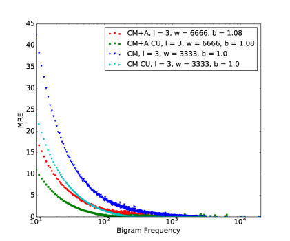
(a)

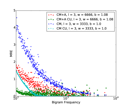
(b)

Figure 5: Experiment measuring mean relative error for bigram estimation. The $y$-value of each point on the plot is equal to the mean relative error for all bigrams whose true frequency is equal to the $x$-value of the point, averaged over $5$ trials; the right figure is the same data zoomed to a subset of the $x$-axis. “CM+A” is a combined sketch using independent counters; “CM+A CU” is a combined sketch with correlated conservative update. “CM CU” and “CM” are conventional sketches with/without conservative update, respectively.

Figure 6 and Figure 7 show the effects of varying the counter base $b$ when using the independent counter and conservative update alternatives. There are two interesting phenomena in these plots. First, when using the independent counters, we see that the error for low frequency words is slightly but consistently lower when the base is larger. This makes sense because we know that the sketch overestimates such words, but when we take the minimum of independent counters the expected value of the result is smaller, which reduces the error for infrequent words – with a larger counter base, it is more likely that the minimum counter happens to underestimate. The second effect is that when using conservative update with a large base, there appear to be more instances with large error when estimating frequent words, compared to the independent case. Again, a plausible explanation is that these errors correspond to cases where the approximate counters occasionally take on a much larger value than the true count, and that when taking the minimum of several independent counters this is unlikely to happen.

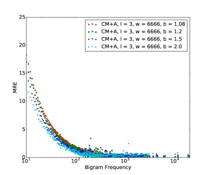
(a)

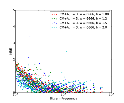
(b)

Figure 6: Effects of different approximate counter base $b$ for bigram estimation benchmark using independent counters. The figure on the right is a zoomed in version of the same data.

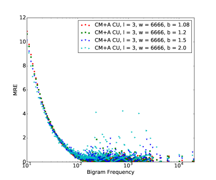
(a)

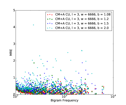
(b)

Figure 7: Effects of different approximate counter base $b$ for bigram estimation benchmark using conservative update.

Figure 8 shows just the points for the $b=2$ conservative update case from these same experiments. There is a noticeable repeating “crisscross” pattern in the errors for the more frequent keys. This arises because the base is so large the counter can only represent counts of the form $2^{k}-1$, so the mean relative error for these keys is largely dependent on how close they are to a value that can be represented in this form.

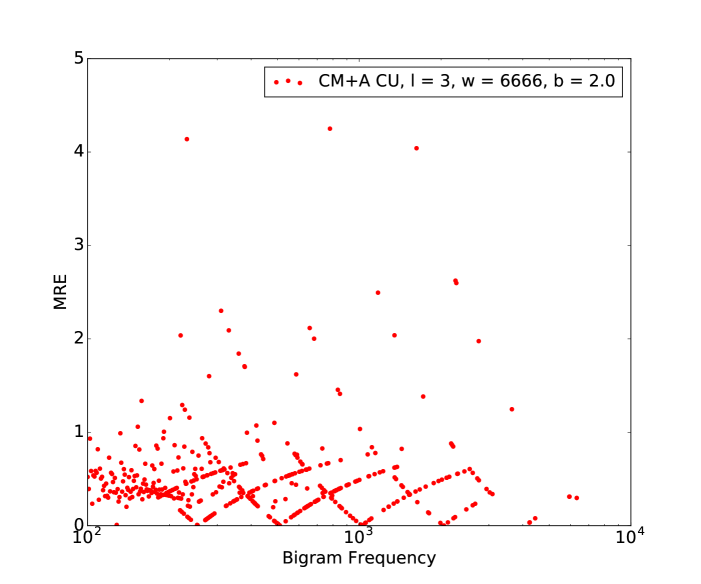
Figure 8: Results showing crisscross pattern for large frequency key errors with large bases.

Finally, Figure 9 shows the error when merging different sketches together. In these experiments, we split the corpus into $k$ substreams of equal size, compute sketches on each, and then merge the $k$ sketches together. We vary $k$ from $1$ to $4$, and use conservative update when computing each of the subsketches. There does not appear to be a substantial difference between the errors when merging or not when using $b=1.08$.

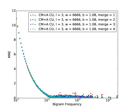
(a)

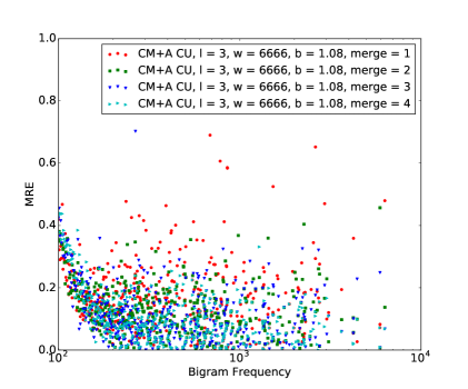
(b)

Figure 9: Effects of merging multiple sketches together using the addition procedure of Steele and Tristan (2016).

Appendix E Experiments

In this section we present additional experiments, provide example topics and report timing results for the various algorithms.

E.1 Example Topics

Since it is possible for a model to have good perplexity, but yield poor topics, we also manually inspect the top-words per topics to ensure that the topics are reasonable in our LDA experiments. In general, we find no perceptible difference in quality between the models that employ sketching and hashing representations of the sufficient statistics and those that employ exact array-based representations. In Table 3 we provide example topics from three different models, all of which use representations that compress the sufficient statistics more than a traditional array of 4-byte integers. The first two systems combine count-min sketch with approximate counters while the third combines all three ideas: count-min sketch, feature hashing and approximate counters. As is typical of LDA and other topic-models, not all topics are perfect and some topics arise out of idiosyncracies of the data like a topic full of dates from a certain century, but again, there did not appear to be noticeable differences in quality between the systems.

Topic A	Topic B	Topic C
CM+A 3 16 1.08
space	episode	law
light	series	court
energy	season	act
system	show	states
earth	episodes	legal
CM+A 3 15 1.04
russian	john	man
war	william	time
government	died	story
soviet	king	series
union	henry	back
CM+H+A 3 18 22 1.08
system	band	court
high	album	police
power	released	case
systems	rock	law
device	records	prison

Table 3: Example topics. “CM+A 3 16 1.08” indicates CM-sketch (three 16-bit hashes) with approximate counters (8-bit base-1.08), “CM+A 3 15 1.04” indicates CM-sketch (three 15-bit hashes) with approximate counters (8-bit base-1.04), and “CM+H+A 3 16 22 1.08” indicates CM-sketch (three 18-bit hashes) with feature hashing (22-bit) and approximate counters (8-bit base-1.08). All three configurations are more compressive than the traditional array-based representation of the sufficient statistics that utilize 4-byte integers.

E.2 Timing results

Method	# hashes	hash range	time (s)
SSCA	NA	NA	12.14 $\pm$ 1.82
SSCAS	3	15	22.75 $\pm$ 4.30
SSCAS	3	16	23.90 $\pm$ 4.41
SSCAS	3	17	25.32 $\pm$ 4.68
SSCAS	3	18	28.10 $\pm$ 5.18
SSCAS	4	15	29.70 $\pm$ 5.82
SSCAS	4	16	32.75 $\pm$ 6.17
SSCAS	4	17	33.35 $\pm$ 5.89
SSCAS	4	18	36.18 $\pm$ 5.97
SSCAS	5	15	37.76 $\pm$ 6.95
SSCAS	5	16	39.71 $\pm$ 7.01
SSCAS	5	17	42.33 $\pm$ 7.75
SSCAS	5	18	45.47 $\pm$ 7.70
SSCAS	6	15	45.04 $\pm$ 8.51
SSCAS	6	16	46.38 $\pm$ 8.18
SSCAS	6	17	48.70 $\pm$ 8.21
SSCAS	6	18	53.03 $\pm$ 8.89
SSCAS	7	15	51.66 $\pm$ 9.45
SSCAS	7	16	53.35 $\pm$ 9.38
SSCAS	7	17	56.44 $\pm$ 9.42
SSCAS	7	18	61.15 $\pm$ 9.93

Table 4: Time per iteration results for LDA with CM sketch.

We report the timing results in this section.

CM sketch timing

Although the CM sketch representation of the sufficient statistics behaves well statistically, there are some computational concerns. In particular, the CM sketch stores multiple counts per word (one per-hash function) and a distributed algorithm must then communicate the extra counts over the network. Therefore, to evaluate the effect on run-time performance, we also report the average per-iteration wall-clock time for each system in Table 4. The method “SSCA” is the default implementation of SCA the employs arrays to represent the sufficient statistics and methods marked “SSCAS” employ the CM sketch.

As expected, the number of hash functions has a bigger impact on running time than the range of the hash functions. Fortunately, at least empirically, the range of the hash function is more important than the number of hash functions in that it has a greater effect on inference’s ability to achieve higher accuracy in fewer iterations. Thus, in terms of both the number of iterations and the wall-clock time, increasing the hash range is more beneficial than increasing the number of hashes.

Timing with approximate counters

Although using the CM sketch with these dimensions increases the running time as demonstrated above, approximate counters effectively compensate for the increased communication overhead because the corresponding sketches are much smaller for a given number of hash functions and range. We report the results in Table 5. The first row, method “SSCA” is the default implementation of SSCA using array representation of the sufficient statistics and “SSCASA” is the version with sketching and approximate counters (8 bits and base 1.08).

Method	# hashes	hash range	time (s)
SSCA	NA	NA	12.14 $\pm$ 1.82
SSCASA	3	15	12.58 $\pm$ 2.00
SSCASA	3	16	17.57 $\pm$ 2.78
SSCASA	3	17	22.69 $\pm$ 3.72
SSCASA	3	18	24.29 $\pm$ 3.93
SSCASA	4	15	17.00 $\pm$ 2.82
SSCASA	4	16	24.50 $\pm$ 4.18
SSCASA	4	17	29.46 $\pm$ 4.88
SSCASA	4	18	32.19 $\pm$ 5.30
SSCASA	5	15	22.11 $\pm$ 3.84
SSCASA	5	16	31.26 $\pm$ 5.54
SSCASA	5	17	37.78 $\pm$ 6.60
SSCASA	5	18	41.12 $\pm$ 6.74

Table 5: Time per iteration results for LDA with CM sketch and approximate counters.

E.3 Exploring more sketching and hashing parameters

In this section, we report a wider range of settings to the parameters of the CM sketch. In particular, we report numbers for a sketch with a range of just 15-bits to one with 18, while also varying the number of hash functions from 3 to 7. To make the plots more readable, we depict curves for sketches with the same hash range in the same color (for example, all sketches with a 15-bit range are red). We also depict curves for sketches with the same number of hash functions with the same symbol (for example, sketches with three hash functions are all marked with circles).

In Figure 10(a) we report the results for just the CM sketch and begin to reach the limits of our ability to push the compressiveness of the sketch. We see that the final perplexity (after 60 iterations) is the same in all cases except for the most compressive variant of the sketch (with 15 bits and 3 hash functions). Since the vocabulary size is 291,561, this sketch is one-third of the size as the raw array-based representation for representing word counts per topic. This seems to be the point at which we begin to see worse final perplexity.

We can also see from this plot that the hash range (curves from the same hash-range are in the same color, and curves with different ranges are in different colors) has a bigger impact on initial performance than the number of hash functions. For example, if we wanted to double the size of the sketch, it would be better to add an extra bit to the range than to double the number of hash functions from 3 to six (as seen by the perplexity gaps in the early iterations between each of the hash ranges). This is in line with the earlier results of Goyal and Daumé III (2011); Goyal et al. (2012).

In Figure 10(b) we repeat the same experiment, but employ an 8-bit base-1.08 approximate counter to represent the counts in the sketch (instead of the usual 4-byte integers). We include up to 5 hashes for this plot. Note that despite using just one-quarter the amount of memory to represent the sufficient statistics, the results for these combined data-structures are similar to the CM sketch alone. Further, as noted earlier, the approximate counters are much faster in a distributed setting since they overcome the additional data that needs to be transmitted by the CM sketch. Thus, the combined data-structure is not only more compressive than the CM sketch alone, but it also runs much faster, achieving similar performance as the original algorithm depending on the setting to its parameters.

Finally, as we mentioned in Section 3, combining the CM sketch and the approximate counters is non-obvious due to the way the min operation interacts with the counters. We had proposed and discussed several alternatives: CM sketch with independent counters, counter min-sketch with correlated counters, and CM sketch with correlated counters and the conservative update rule to reduce the bias. We show the plots for these counters in Figures 11, 12, 13 respectively. We also vary the base of the counters while keeping the number of counter bits fixed at 8. Each color represents a different base (1.08, 1.09 and 1.10) to make it easier to interpret. The main takeaways from these plots is that the method in which you combine the counters and min-sketch does not matter as much for an application like LDA, which seems to be robust to the bias in the first two methods. We note that in some cases, increasing the base of the counter appears to improve perplexity. While we have not been able to find a satisfactory explanation for this phenomenon, previous work on the geometric aspects of topic modeling Yurochkin and Nguyen (2016); Yurochkin et al. (2017) has highlighted the subtle interaction between the geometry of the topic simplex and perplexity.

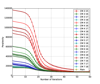
(a) CM sketch only

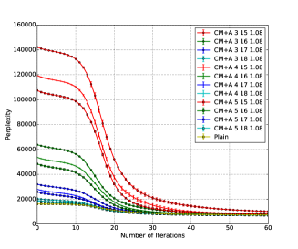
(b) sketch + approx. counters

Figure 10: Experiments across a full range of parameter settings for the sketch.

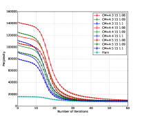
(a) 15 bits

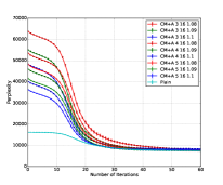
(b) 16 bits

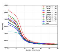
(c) 17 bits

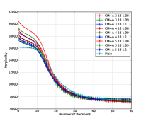
(d) 18 bits

Figure 11: Independent counter variant of the combined CM sketch and approximate counter data-structure on LDA with a hash range of 15,16,17 and 18 as indicated in the respective captions.

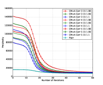
(a) 15 bits

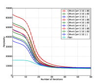
(b) 16 bits

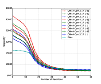
(c) 17 bits

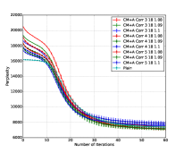
(d) 18 bits

Figure 12: Correlated counter variant of the combined CM sketch and approximate counter data-structure on LDA with a hash range of 15,16,17 and 18 as indicated in the respective captions.

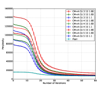
(a) 15 bits

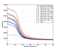
(b) 16 bits

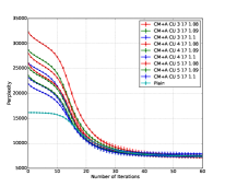
(c) 17 bits

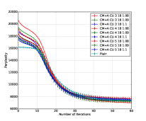
(d) 18 bits

Figure 13: Correlated counter + conservative update variant of the combined CM sketch and approximate counter data-structure on LDA with a hash range of 15,16,17 and 18 as indicated in the respective captions.

References

- Alquier et al. (2014) P. Alquier, N. Friel, R. Everitt, and A. Boland. Noisy Monte Carlo: Convergence of Markov chains with approximate transition kernels. ArXiv e-prints, March 2014.
- Angelino et al. (2016) Elaine Angelino, Matthew James Johnson, and Ryan P. Adams. Patterns of scalable bayesian inference. Foundations and Trends in Machine Learning, 9(2-3):119–247, 2016.
- Bardenet et al. (2014) Rémi Bardenet, Arnaud Doucet, and Christopher C. Holmes. Towards scaling up markov chain monte carlo: an adaptive subsampling approach. In Proceedings of the 31th International Conference on Machine Learning, ICML 2014, Beijing, China, 21-26 June 2014, pages 405–413, 2014.
- Blei et al. (2003) David M. Blei, Andrew Y. Ng, and Michael I. Jordan. Latent dirichlet allocation. J. Mach. Learn. Res., 3:993–1022, March 2003.
- Chen et al. (2016) Jianfei Chen, Kaiwei Li, Jun Zhu, and Wenguang Chen. Warplda: A cache efficient o(1) algorithm for latent dirichlet allocation. Proc. VLDB Endow., 9(10):744–755, June 2016. ISSN 2150-8097.
- Cormode and Muthukrishnan (2005) Graham Cormode and S. Muthukrishnan. An improved data stream summary: The count-min sketch and its applications. J. Algorithms, 55(1):58–75, April 2005. ISSN 0196-6774.
- Deng and Rafiei (2007) Fan Deng and Davood Rafiei. New estimation algorithms for streaming data: Count-min can do more, 2007.
- Durme and Lall (2009a) Benjamin Van Durme and Ashwin Lall. Streaming pointwise mutual information. In Advances in Neural Information Processing Systems 22: 23rd Annual Conference on Neural Information Processing Systems 2009. Proceedings of a meeting held 7-10 December 2009, Vancouver, British Columbia, Canada., pages 1892–1900, 2009a.
- Durme and Lall (2009b) Benjamin Van Durme and Ashwin Lall. Probabilistic counting with randomized storage. In IJCAI 2009, Proceedings of the 21st International Joint Conference on Artificial Intelligence, Pasadena, California, USA, July 11-17, 2009, pages 1574–1579, 2009b.
- Estan and Varghese (2002) Cristian Estan and George Varghese. New directions in traffic measurement and accounting. In Proceedings of the ACM SIGCOMM 2002 Conference on Applications, Technologies, Architectures, and Protocols for Computer Communication, August 19-23, 2002, Pittsburgh, PA, USA, pages 323–336, 2002.
- Flajolet (1985) Philippe Flajolet. Approximate counting: A detailed analysis. BIT, 25(1):113–134, June 1985.
- Geppert et al. (2017) Leo N. Geppert, Katja Ickstadt, Alexander Munteanu, Jens Quedenfeld, and Christian Sohler. Random projections for bayesian regression. Statistics and Computing, 27(1):79–101, 2017.
- Goyal and Daumé III (2011) Amit Goyal and Hal Daumé III. Approximate scalable bounded space sketch for large data NLP. In EMNLP, pages 250–261, 2011.
- Goyal et al. (2012) Amit Goyal, Hal Daumé III, and Graham Cormode. Sketch algorithms for estimating point queries in NLP. In EMNLP-CoNLL, pages 1093–1103, 2012.
- Gumbel (1954) E. J. Gumbel. The maxima of the mean largest value and of the range. The Annals of Mathematical Statistics, 25(1):76–84, 1954. ISSN 00034851. URL http://www.jstor.org/stable/2236513.
- Hartley and David (1954) H. O. Hartley and H. A. David. Universal bounds for mean range and extreme observation. Ann. Math. Statist., 25(1):85–99, 03 1954. doi: 10.1214/aoms/1177728848. URL https://doi.org/10.1214/aoms/1177728848.
- Huggins et al. (2016) Jonathan H. Huggins, Trevor Campbell, and Tamara Broderick. Coresets for scalable bayesian logistic regression. In Advances in Neural Information Processing Systems 29: Annual Conference on Neural Information Processing Systems 2016, December 5-10, 2016, Barcelona, Spain, pages 4080–4088, 2016.
- Karr (1975) Alan F. Karr. Weak convergence of a sequence of markov chains. Wahrscheinlichkeitstheorie verw Gebiete, 35(1):41–48, 1975.
- Li et al. (2017) Kaiwei Li, Jianfei Chen, Wenguang Chen, and Jun Zhu. Saberlda: Sparsity-aware learning of topic models on gpus. In ASPLOS, pages 497–509, 2017. ISBN 978-1-4503-4465-4.
- Li and McCallum (2006) Wei Li and Andrew McCallum. Pachinko allocation: Dag-structured mixture models of topic correlations. In International Conference on Machine Learning, 2006.
- Lindvall (2002) Torgny Lindvall. Lectures on the Coupling Method. Dover Books on Mathematics Series. Dover Publications, Incorporated, 2002. ISBN 9780486421452.
- Morris (1978) Robert Morris. Counting large numbers of events in small registers. Commun. ACM, 21(10):840–842, October 1978. ISSN 0001-0782. doi: 10.1145/359619.359627. URL http://doi.acm.org/10.1145/359619.359627.
- Negrea and Rosenthal (2017) J. Negrea and J. S. Rosenthal. Error Bounds for Approximations of Geometrically Ergodic Markov Chains. ArXiv e-prints, February 2017.
- Pillai and Smith (2014) N. S. Pillai and A. Smith. Ergodicity of Approximate MCMC Chains with Applications to Large Data Sets. ArXiv e-prints, May 2014.