Numerical Methods for the Magnetic Induction Equation with Hall Effect and Projections onto Divergence-Free Vector Fields

Abstract

The nonlinear magnetic induction equation with Hall effect can be used to model magnetic fields, e.g. in astrophysical plasma environments. In order to give reliable results, numerical simulations should be carried out using effective and efficient schemes. Thus, high-order stable schemes are investigated here.

Following the approach provided recently by Nordström (J Sci Comput 71.1, pp. 365–385, 2017), an energy analysis for both the linear and the nonlinear induction equation including boundary conditions is performed at first. Novel outflow boundary conditions for the Hall induction equation are proposed, resulting in an energy estimate. Based on an energy analysis of the initial boundary value problem at the continuous level, semidiscretisations using summation by parts (SBP) operators and simultaneous approximation terms are created. Mimicking estimates at the continuous level, several energy stable schemes are obtained in this way and compared in numerical experiments. Moreover, stabilisation techniques correcting errors in the numerical divergence of the magnetic field via projection methods are studied from an energetic point of view in the SBP framework. In particular, the treatment of boundaries is investigated and a new approach with some improved properties is proposed.

1 Introduction

Numerical plasma simulations have many applications not only in space physics, but also in engineering. In recent years increasingly powerful computers have caused a quick adoption of different numerical models to simulate the interaction of the solar wind with different celestial objects [38, 31], space weather [85], and the performance of plasma engines [5, 53]. While advances in computational power and available memory have allowed for increasingly accurate physical models with higher spatial and temporal accuracy, the numerical methods used to solve the underlying equations have started to become a limiting factor. In the past numerical instabilities and other artefacts were commonly small compared to the errors introduced by insufficient physical modelling, but with increased model quality and accuracy, shortcomings in the numerical methods became noticeable.

This article is concerned with the numerical treatment of one of the primary equations behind all numeric plasma models: the magnetic induction equation. It is widely used in different models, except some completely kinetic approaches, and is usually written in non-dimensional form as

$$\partial_{t}B=\underbrace{\nabla\times(u\times B)}_{\text{transport term}}\underbrace{-\nabla\times\biggl{(}\frac{\nabla\times B}{\varrho}\times B\biggr{)}}_{\text{Hall term}},$$ (1)

where $B$ is the magnetic field, $u$ the particle velocity, $\varrho$ the particle charge density, and $\nabla\times B$ the curl of $B$. If not mentioned otherwise, all functions depend on time $t\in(0,T)$ and space $x=(x_{1},x_{2},x_{3})\in\Omega\subseteq\mathbb{R}^{3}$. The first term on the right hand side of (1) is often called transport term and the second one is the Hall term. In general, the induction equation (1) is supplemented with the divergence constraint $\operatorname{div}B=0$ on the magnetic field. Of course, suitable initial and boundary conditions have to be given.

The induction equation (1) can be used as part of larger physical models, in particular magnetohydrodynamics (MHD). Then, there are additional equations determining the particle charge density and velocity. Considering the induction equation (1) as a model on its own, the quantities $u$ and $\varrho$ are given data. While the Hall term on the right hand side of (1) can be dropped for some applications, many MHD models require it to accurately describe processes such as the evolution of the protostellar disk [17, 75] or the comet solar wind interaction [31]. Other terms may also be added to extend the model and describe additional physical processes governed primarily by resistive or electron inertia effects. Using $\operatorname{div}(\nabla\times\cdot)=0$, the divergence constraint $\operatorname{div}B=0$ will be automatically fulfilled if the initial condition $B^{0}$ satisfies it, all functions are sufficiently smooth, and boundaries are ignored.

The magnetic induction equation (1) has been considered in different forms in the literature. In [22, 23, 40, 50], only the transport term has been considered. A linear resistive term has been added in [39]. Another variant of the induction equation with Hall effect without discussion of boundary conditions has been investigated in [12].

The fundamental technique used in this article is the energy method, cf. [28, chapters 8 and 11]. Physically, it can be motivated as follows. The magnetic energy is proportional to $\mathinner{\!\left\lvert B\right\rvert}^{2}$ and fulfils a secondary balance law that can be determined using the induction equation (1), since $\partial_{t}\mathinner{\!\left\lvert B\right\rvert}^{2}=2B\cdot\partial_{t}B$ for sufficiently smooth solutions. Boundary conditions have to be given such that the magnetic energy remains bounded and can be estimated by given initial and boundary data. This behaviour should hold for both the partial differential equation (PDE) at the continuous level and the discrete variant.

Following the approach of [54], in order to know what should be mimicked by the discretisation, the initial boundary value problem (IBVP) will be investigated at first at the continuous level. Results obtained there are also useful on their own and can be applied to different discretisations, not only the ones considered in this article. Boundary conditions will be imposed both strongly (i.e. by enforcing given boundary values exactly) and weakly (i.e. by adding an appropriate penalty term to the PDE).

In order to mimic estimates obtained from the energy method semidiscretely, summation by parts (SBP) derivative operators will be used [44, 79]. The weak imposition of boundary conditions is mimicked via simultaneous approximation terms (SATs) [8, 9]. Further information can be found in the review articles [82, 19] and references cited therein. One method to obtain energy estimates for problems with varying coefficients or nonlinear ones is the application of certain splittings. Such techniques have been used successfully in the literature, cf. [62, 93, 74, 55, 37, 51, 76, 41, 25, 91, 67, 71, 78, 77].

Although SBP operators have been developed in the context of finite difference (FD) methods and this setting will be used here, they can also be found in various other frameworks including finite volume (FV) [57, 58], discontinuous Galerkin (DG) [24, 18], and the recent flux reconstruction/correction procedure via reconstruction schemes [33, 34, 72]. Thus, basic results about energy estimates and boundary conditions obtained here can also be applied to these schemes.

This article is structured as follows. At first, the linear magnetic induction equation using only the transport term is investigated in section 2. After the derivation of energy estimates and admissible boundary conditions, the concept of SBP operators is briefly reviewed and applied to obtain stable semidiscretisations. Afterwards, the nonlinear induction equation with Hall effect is considered in section 3. Using the same basic approach, energy stable outflow boundary conditions are proposed and studied both at the continuous and the semidiscrete level. In section 4, the focus lies on the divergence constraint. Since it has been used widely, the projection method enforcing this constraint is studied from the point of view of the energy method and corresponding boundary conditions are investigated. Thereafter, results of numerical experiments are presented in section 5. Finally, a summary and discussion of the obtained results is given in section 6.

2 Linear Magnetic Induction Equation

This section is focused on the transport term of the magnetic induction equation (1). Thus, the linear equation

$$\partial_{t}B=\nabla\times(u\times B)$$ (2)

with divergence constraint $\operatorname{div}B=0$ and suitable initial and boundary conditions will be investigated. Therefore, the PDE will be rewritten using the divergence constraint such that the energy rate can be calculated via

$$\dfrac{\operatorname{d\!}{}}{\operatorname{d\!}{t}}\mathinner{\!\left\lVert B\right\rVert}_{L^{2}(\Omega)}^{2}=\dfrac{\operatorname{d\!}{}}{\operatorname{d\!}{t}}\int_{\Omega}\mathinner{\!\left\lvert B\right\rvert}^{2}=2\int_{\Omega}B\cdot\partial_{t}B$$ (3)

and inserting the PDE, leading to admissible boundary conditions. Implementing these in a weak form yields an energy estimate involving given initial and boundary data. Finally, using summation by parts operators, a semidiscretisation mimicking these properties will be constructed.

2.1 Continuous Setting

The $i$-th component of the transport term $\nabla\times(u\times B)$ can be written using the totally antisymmetric Levi-Civita symbol $\varepsilon_{ijk}$ as

$$\left[\nabla\times(u\times B)\right]_{i}=\varepsilon_{ijk}\partial_{j}\bigl{(}\varepsilon_{klm}u_{l}B_{m}\bigr{)}=\partial_{j}\bigl{(}u_{i}B_{j}-u_{j}B_{i}\bigr{)},$$ (4)

where summation over repeated indices is implied. In order to obtain an energy estimate, the product rule can be used to rewrite the transport term as

$$\partial_{j}\bigl{(}u_{i}B_{j}-u_{j}B_{i}\bigr{)}=\underbrace{u_{i}\partial_{j}B_{j}}_{(i)}\underbrace{+B_{j}\partial_{j}u_{i}-\frac{1}{2}B_{i}\partial_{j}u_{j}}_{(ii)}\underbrace{-\frac{1}{2}u_{j}\partial_{j}B_{i}-\frac{1}{2}\partial_{j}(u_{j}B_{i})}_{(iii)}.$$ (5)

If $\operatorname{div}B=0$, the first term $(i)$ on the right hand side vanishes. Dropping it can in general be interpreted as adding $-u\operatorname{div}B$ to the right hand side of the magnetic induction equation (2), as studied in [27, 64, 65] for the MHD equations. Investigations in the context of numerical schemes for the induction equation can be found in [22, 40, 50]. Without dropping the term $(i)$, the system is not symmetric. Moreover, it cannot be symmetrised, and the energy method cannot be applied, cf. [50] for the two-dimensional case.

The terms $(ii)$ of (5) contain no derivatives of the magnetic field and can be interpreted as source terms describing the influence of the particles on the magnetic field. The remaining terms $(iii$) contain derivatives of $B$. Multiplying by the magnetic field and integrating over a volume $\Omega$ such that the divergence theorem can be used yields

$$\int_{\Omega}B\cdot\partial_{t}B =\int_{\Omega}\left(B_{i}B_{j}\partial_{j}u_{i}-\frac{1}{2}B_{i}B_{i}\partial_{j}u_{j}-\frac{1}{2}B_{i}u_{j}\partial_{j}B_{i}-\frac{1}{2}B_{i}\partial_{j}(u_{j}B_{i})\right)$$ (6)

$$=\int_{\Omega}\left(B_{i}B_{j}\partial_{j}u_{i}-\frac{1}{2}B_{i}B_{i}\partial_{j}u_{j}\right)-\int_{\partial\Omega}\frac{1}{2}B_{i}B_{i}u_{j}\nu_{j},$$

where $\nu=(\nu_{j})_{j}$ is the outward unit normal at $\partial\Omega$. This proves

Lemma 2.1.

If the linear induction equation (2) is written in the form

$$\partial_{t}B_{i}=B_{j}\partial_{j}u_{i}-\frac{1}{2}B_{i}\partial_{j}u_{j}-\frac{1}{2}u_{j}\partial_{j}B_{i}-\frac{1}{2}\partial_{j}(u_{j}B_{i}),$$ (7)

the energy rate can be obtained using only integration by parts via

$$\int_{\Omega}B\cdot\partial_{t}B=\int_{\Omega}\left(B_{i}B_{j}\partial_{j}u_{i}-\frac{1}{2}B_{i}B_{i}\partial_{j}u_{j}\right)-\int_{\partial\Omega}\frac{1}{2}B_{i}B_{i}u_{j}\nu_{j}.$$ (8)

Following classical arguments for linear PDEs, boundary conditions should be given such that an energy estimate can be obtained, cf. [54]. Concentrating on the surface term in (8), an energy growth can only occur if $u_{j}\nu_{j}=u\cdot\nu<0$. Since $\nu$ is the outward normal and $u$ the particle velocity, this corresponds exactly to the case of an inflow, in accordance with physical intuition and the frozen in theorem [1]. Thus, the initial boundary value problem for the induction equation (7) becomes

$$\partial_{t}B_{i} =B_{j}\partial_{j}u_{i}-\frac{1}{2}B_{i}\partial_{j}u_{j}-\frac{1}{2}u_{j}\partial_{j}B_{i}-\frac{1}{2}\partial_{j}(u_{j}B_{i}), \text{in }(0,T)\times\Omega,$$ (9)

$$B(t,x) =B^{b}(t,x), \text{if }u(t,x)\cdot\nu(x)<0\text{ on }\partial\Omega,$$

$$B(0,x) =B^{0}(x), x\in\Omega,$$

where $B^{0}$ and $B^{b}$ are given initial and boundary data. Using these supplementary conditions, the magnetic energy can be estimated as follows.

Lemma 2.2.

A sufficiently smooth solution $B$ of the linear induction equation (9) fulfils

$$\dfrac{\operatorname{d\!}{}}{\operatorname{d\!}{t}}\mathinner{\!\left\lVert B(t)\right\rVert}_{L^{2}(\Omega)}^{2}=2\int_{\Omega}B\cdot\partial_{t}B\leq 9\mathinner{\!\left\lVert\nabla u(t)\right\rVert}_{L^{\infty}(\Omega)}\mathinner{\!\left\lVert B(t)\right\rVert}_{L^{2}(\Omega)}^{2}+\mathinner{\!\left\lVert u(t)\right\rVert}_{L^{\infty}(\partial\Omega)}\mathinner{\!\left\lVert B^{b}(t)\right\rVert}_{L^{2}(\partial\Omega)}^{2}$$ (10)

and

$$\mathinner{\!\left\lVert B(t)\right\rVert}_{L^{2}(\Omega)}^{2}\leq\exp\bigl{(}9\mathinner{\!\left\lVert\nabla u\right\rVert}_{\infty}t\bigr{)}\left(\mathinner{\!\left\lVert B^{0}\right\rVert}_{L^{2}(\Omega)}^{2}+\int_{0}^{t}\mathinner{\!\left\lVert u(t)\right\rVert}_{L^{\infty}(\partial\Omega)}\mathinner{\!\left\lVert B^{b}(t)\right\rVert}_{L^{2}(\partial\Omega)}^{2}\operatorname{d\!}t\right).$$ (11)

Proof.

If the particle velocity $u$ and its partial derivatives are bounded, the energy rate can be estimated using (8) via

$$\int_{\Omega}B\cdot\partial_{t}B =\int_{\Omega}\left(B_{i}B_{j}\partial_{j}u_{i}-\frac{1}{2}B_{i}B_{i}\partial_{j}u_{j}\right)-\int_{\partial\Omega}\frac{1}{2}B_{i}B_{i}u_{j}\nu_{j}$$ (12)

$$\leq\mathinner{\!\left\lVert\nabla u(t)\right\rVert}_{L^{\infty}(\Omega)}\sum_{i,j}\int_{\Omega}\mathinner{\!\left\lvert B_{i}\right\rvert}\mathinner{\!\left\lvert B_{j}\right\rvert}+\frac{3}{2}\mathinner{\!\left\lVert\nabla u(t)\right\rVert}_{L^{\infty}(\Omega)}\int_{\Omega}\mathinner{\!\left\lvert B\right\rvert}^{2}+\frac{1}{2}\mathinner{\!\left\lVert u(t)\right\rVert}_{L^{\infty}(\partial\Omega)}\int_{\partial\Omega}\mathinner{\!\left\lvert B^{b}\right\rvert}^{2}.$$

For this estimate, the boundary $\partial\Omega$ has been divided into two parts: the inflow part $\partial\Omega_{\mathrm{in}}$ (where $u\cdot\nu<0$) and the outflow part $\partial\Omega_{\mathrm{out}}$ (where $u\cdot\nu\geq 0$). On $\partial\Omega_{\mathrm{in}}$, the boundary condition $B=B^{b}$ has been inserted. The integral over $\partial\Omega_{\mathrm{out}}$ is non-positive, since $B_{i}B_{i}u_{j}\nu_{j}=\mathinner{\!\left\lvert B\right\rvert}^{2}u\cdot\nu\geq 0$ there. The infinity norm is $\mathinner{\!\left\lVert\nabla u(t)\right\rVert}_{L^{\infty}(\Omega)}=\max_{i,j}\mathinner{\!\left\lVert\partial_{j}u_{i}(t)\right\rVert}_{L^{\infty}(\Omega)}$. Using

$$\sum_{i,j}\int_{\Omega}\mathinner{\!\left\lvert B_{i}\right\rvert}\mathinner{\!\left\lvert B_{j}\right\rvert}\leq\sum_{i,j}\int_{\Omega}\frac{1}{2}\Bigl{(}\mathinner{\!\left\lvert B_{i}\right\rvert}^{2}+\mathinner{\!\left\lvert B_{j}\right\rvert}^{2}\Bigr{)}=3\mathinner{\!\left\lVert B\right\rVert}_{L^{2}(\Omega)}^{2}$$ (13)

yields

$$\int_{\Omega}B\cdot\partial_{t}B\leq\frac{9}{2}\mathinner{\!\left\lVert\nabla u(t)\right\rVert}_{L^{\infty}(\Omega)}\mathinner{\!\left\lVert B(t)\right\rVert}_{L^{2}(\Omega)}^{2}+\frac{1}{2}\mathinner{\!\left\lVert u(t)\right\rVert}_{L^{\infty}(\partial\Omega)}\mathinner{\!\left\lVert B^{b}(t)\right\rVert}_{L^{2}(\partial\Omega)}^{2}.$$ (14)

Abbreviating $\mathinner{\!\left\lVert\nabla u\right\rVert}_{\infty}=\max_{i,j}\mathinner{\!\left\lVert\partial_{j}u_{i}\right\rVert}_{L^{\infty}((0,T)\times\Omega)}$, the energy estimate (11) follows due to Grönwall’s inequality. ∎

Instead of the strong implementation of the boundary conditions as in (9), the boundary conditions can also be implemented in a weak form. Since this form is related directly to semidiscretisations using SBP operators and SATs, it will be used in the following. Therefore, a lifting operator $L$ is used. Similar to a Dirac measure concentrated on the boundary $\partial\Omega$, it fulfils

$$\int_{\Omega}u\cdot L(\psi)=\int_{\partial\Omega}\varphi\cdot\psi$$ (15)

for smooth (and possibly vector valued) functions $\varphi,\psi$, cf. [2, 90, 54]. In the semidiscrete setting, such a lifting operator is mainly given by a multiplication by the inverse grid size as described in the following subsection. Imposing the boundary data $B^{b}$ weakly yields the IBVP

$$\partial_{t}B_{i} =B_{j}\partial_{j}u_{i}-\frac{1}{2}B_{i}\partial_{j}u_{j}-\frac{1}{2}u_{j}\partial_{j}B_{i}-\frac{1}{2}\partial_{j}(u_{j}B_{i})$$ (16)

$$\phantom{=}+L\bigl{(}\mathbbm{1}_{\left\{u\cdot\nu<0\right\}}(u\cdot\nu)(B_{i}-B^{b}_{i})\bigr{)}, \text{in }(0,T)\times\Omega,$$

$$B(0,x) =B^{0}(x), x\in\Omega,$$

where $\mathbbm{1}_{\left\{u\cdot\nu<0\right\}}$ is one where $u\cdot\nu<0$ and zero elsewhere. Similar to the strong form of the boundary conditions, this yields

Lemma 2.3.

A sufficiently smooth solution $B$ of the linear induction equation (16) with weak implementation of the boundary condition satisfies the energy estimate for the strong implementation given in Lemma 2.2. If the boundary condition is not fulfilled exactly, there is an additional dissipative term.

Proof.

As in the proof of Lemma 2.2, the energy rate can be estimated using (8) via

$$\int_{\Omega}B\cdot\partial_{t}B=\int_{\Omega}\left(B_{i}B_{j}\partial_{j}u_{i}-\frac{1}{2}B_{i}B_{i}\partial_{j}u_{j}\right)-\int_{\partial\Omega}\frac{1}{2}B_{i}B_{i}u_{j}\nu_{j}+\int_{\Omega}B_{i}L\bigl{(}\mathbbm{1}_{\left\{u\cdot\nu<0\right\}}u_{j}\nu_{j}(B_{i}-B^{b}_{i})\bigr{)}.$$ (17)

Only the last term on the right hand side is new and can be rewritten as

$$\int_{\Omega}B_{i}L\bigl{(}\mathbbm{1}_{\left\{u\cdot\nu<0\right\}}u_{j}\nu_{j}(B_{i}-B^{b}_{i})\bigr{)}=\int_{\partial\Omega}\mathbbm{1}_{\left\{u\cdot\nu<0\right\}}u_{j}\nu_{j}B_{i}(B_{i}-B^{b}_{i}).$$ (18)

Thus, the surface terms are

$$-\int_{\partial\Omega}\left(\frac{1}{2}B_{i}B_{i}u_{j}\nu_{j}-\mathbbm{1}_{\left\{u\cdot\nu<0\right\}}u_{j}\nu_{j}B_{i}(B_{i}-B^{b}_{i})\right)=-\int_{\partial\Omega}u_{j}\nu_{j}\left(\frac{1}{2}B_{i}B_{i}-\mathbbm{1}_{\left\{u\cdot\nu<0\right\}}(B_{i}B_{i}-B_{i}B^{b}_{i})\right).$$ (19)

The integrand is the same as for the strong implementation of the boundary conditions where $u\cdot\nu\geq 0$, i.e. $-u_{j}\nu_{j}B_{i}B_{i}\leq 0$. Elsewhere, the integrand is

$$-u_{j}\nu_{j}\left(\frac{1}{2}B_{i}B_{i}-(B_{i}B_{i}-B_{i}B^{b}_{i})\right)=-\frac{1}{2}u_{j}\nu_{j}B^{b}_{i}B^{b}_{i}+\frac{1}{2}\underbrace{u_{j}\nu_{j}}_{<0}(B_{i}-B^{b}_{i})(B_{i}-B^{b}_{i})\leq-\frac{1}{2}u_{j}\nu_{j}B^{b}_{i}B^{b}_{i}.$$ (20)

Hence, an additional dissipative term

$$-\int_{\partial\Omega}\mathbbm{1}_{\left\{u\cdot\nu<0\right\}}u_{j}\nu_{j}(B_{i}-B^{b}_{i})(B_{i}-B^{b}_{i})\leq 0$$ (21)

appears in the estimate of the energy rate $\dfrac{\operatorname{d\!}{}}{\operatorname{d\!}{t}}\mathinner{\!\left\lVert B(t)\right\rVert}_{L^{2}(\Omega)}^{2}$ compared to the strong form of the boundary condition. ∎

2.2 Summation by Parts Operators

Using the formulation (16) of the magnetic induction equation with weak implementation of the boundary condition, the estimates of the energy rate (10) and of the energy (11) have been obtained using only integration by parts and properties of the lifting operator $L$. Thus, these have to be mimicked discretely in order to obtain similar estimates at the semidiscrete level. Summation by parts operators and simultaneous approximation terms are these discrete analogues.

Before presenting a semidiscretisation of (16), the concept of SBP operators will be described briefly. Since finite difference methods on Cartesian grids will be used in the following, the one dimensional setting is described at first.

The given domain $\Omega=[x_{L},x_{R}]$ is discretised as a uniform grid with nodes $x_{L}=x_{1}<x_{2}<\dots<x_{N}=x_{R}$. A function $u$ is represented discretely as a vector $(u^{(a)})_{a}$, where the components are the values at the grid nodes, i.e. $u^{(a)}=u(x_{a})$. Nonlinear operations are performed componentwise. Thus, the product of two functions $u$ and $v$ is represented by the Hadamard product of the corresponding vectors, i.e. $(uv)^{(a)}=u^{(a)}v^{(a)}$. By a slight abuse of notation, $u$ may represent the vector of coefficients or the diagonal multiplication matrix $\operatorname{diag}\left(u\right)$, performing this multiplication of discretised functions.

Since summation by parts should mimic integration by parts, derivatives and integrals have to be discretised. Therefore, the derivative operator is represented by a matrix $D$, i.e. $Du\approx\partial_{x}u$. The integral over $\Omega$ is interpreted as the $L^{2}$ scalar product and represented by a symmetric and positive definite norm/mass matrix $M$, i.e.

$$u^{T}Mv=\left\langle{u,\,v}\right\rangle_{M}\approx\left\langle{u,\,v}\right\rangle_{L^{2}(\Omega)}=\int_{\Omega}u\cdot v.$$ (22)

Since boundary nodes are included, integration with respect to the outer unit normal $\nu$ at $\partial\Omega$ as in the divergence theorem is given by the difference of boundary values. This bilinear form is represented by the matrix $E=\operatorname{diag}\left(-1,0,\dots,0,1\right)$. Together, these operators mimic integration by parts discretely via

$$\begin{array}[]{ccc}\underbrace{u^{T}MDv+u^{T}D^{T}Mv}&=&\underbrace{u^{T}Ev,}\\ \rotatebox{90.0}{$\!\approx\;$}&&\rotatebox{90.0}{$\!\!\approx\;$}\\ \overbrace{\int_{x_{L}}^{x_{R}}u\,(\partial_{x}v)+\int_{x_{L}}^{x_{R}}(\partial_{x}u)\,v}&=&\overbrace{u\,v\big{|}_{x_{L}}^{x_{R}}},\end{array}$$ (26)

if the SBP property

$$MD+D^{T}M=E$$ (27)

is fulfilled. Finally, the discrete version of the lifting operator $L$ is $M^{-1}\mathinner{\!\left\lvert E\right\rvert}$, since

$$\int_{\Omega}u\cdot L(v)\approx u^{T}M\left(M^{-1}\mathinner{\!\left\lvert E\right\rvert}v\right)=u^{T}\mathinner{\!\left\lvert E\right\rvert}v=\bigl{(}u^{(N)}\cdot v^{(N)}+u^{(1)}\cdot v^{(1)}\bigr{)}\approx\int_{\partial\Omega}u\cdot v.$$ (28)

Here, only diagonal norm SBP operators are considered, i.e. those SBP operators with diagonal mass matrices $M$. In this case, discrete integrals are evaluated using the quadrature provided by the weights of the diagonal mass matrix. For classical diagonal norm SBP operators, the order of accuracy is $2p$ in the interior and $p$ at the boundaries, allowing a global convergence order of $p+1$ for hyperbolic problems [81, 80]. Here, SBP operators will be referred to by their interior order of accuracy $2p$.

Example 2.4.

The classical second order accurate SBP operators are

$$D=\frac{1}{2\Delta x}\begin{pmatrix}-2&2\\ -1&0&1\\ &\ddots&\ddots&\ddots\\ &&-1&0&1\\ &&&-2&2\end{pmatrix},\qquad M=\Delta x\begin{pmatrix}\frac{1}{2}\\ &1\\ &&\ddots\\ &&&1\\ &&&&\frac{1}{2}\end{pmatrix},$$ (29)

where $\Delta x$ is the grid spacing. Thus, the first derivative is given by the standard second order central derivative in the interior and by one sided derivative approximations at the boundaries.

In multiple space dimensions, tensor product operators will be used, i.e. the one dimensional SBP operators are applied accordingly in each dimension. Thus, they are of the form

$$D_{1}=D_{x}\otimes\operatorname{I}_{y}\otimes\operatorname{I}_{z},\quad D_{2}=\operatorname{I}_{x}\otimes D_{y}\otimes\operatorname{I}_{z},\quad D_{3}=\operatorname{I}_{x}\otimes\operatorname{I}_{y}\otimes D_{z},$$ (30)

where $\operatorname{I}_{x,y,z}$ are identity matrices and $D_{x,y,z}$ are one dimensional SBP derivative operators in the corresponding coordinate directions. The boundary operators are

$$E_{1}=E_{x}\otimes M_{y}\otimes M_{z},\quad E_{2}=M_{x}\otimes E_{y}\otimes M_{z},\quad E_{3}=M_{x}\otimes M_{y}\otimes E_{z}.$$ (31)

They fulfil $u^{T}E_{i}v\approx\int_{\partial\Omega}u\cdot v\,\nu_{i}$. Sometimes, the boundary integral operator

$$E=\mathinner{\!\left\lvert E_{1}\right\rvert}+\mathinner{\!\left\lvert E_{2}\right\rvert}+\mathinner{\!\left\lvert E_{3}\right\rvert}$$ (32)

will be used. Finally, the mass matrix is $M=M_{x}\otimes M_{y}\otimes M_{z}$.

Remark 2.5.

The standard tensor product discretisations of the divergence and curl operators given above satisfy $\operatorname{div}\operatorname{curl}=0$, since the discrete derivative operators commute, i.e. $D_{j}D_{i}=D_{i}D_{j}$. However, the imposition of boundary conditions has to be taken into account. Thus, the discrete divergence of the magnetic field will not remain zero, even if the initial data are discretely divergence free. Hence, even the direct discretisation of the conservative form of $\nabla\times(u\times B)$ without source term will not result in discretely divergence free magnetic fields. Thus, the divergence constraint will be considered in more detail in section 4.

2.3 Semidiscrete Setting

Replacing derivatives $\partial_{j}$ by SBP operators $D_{j}$ and the lifting operator of terms multiplied by $\nu_{j}$ by $M^{-1}E_{j}$ results in the following semidiscretisation of the linear induction equation (16) with weak implementation of the boundary conditions.

$$\partial_{t}B_{i} =B_{j}D_{j}u_{i}-\frac{1}{2}B_{i}D_{j}u_{j}-\frac{1}{2}u_{j}D_{j}B_{i}-\frac{1}{2}D_{j}(u_{j}B_{i})$$ (33)

$$\phantom{=}+M^{-1}E_{j}\bigl{(}\mathbbm{1}_{\left\{u\cdot\nu<0\right\}}u_{j}(B_{i}-B^{b}_{i})\bigr{)}, \text{for }t\in(0,T),$$

$$B(0) =B^{0}.$$

Remark 2.6.

The surface term in (33) can also be written using numerical fluxes as in finite volume and discontinuous Galerkin methods. Indeed,

$$\mathbbm{1}_{\left\{u\cdot\nu<0\right\}}u_{j}(B_{i}-B^{b}_{i})=u_{j}B_{i}-u_{j}B^{\mathrm{num}}_{i},$$ (34)

where $B^{\mathrm{num}}$ is the upwind numerical flux, i.e. $B^{\mathrm{num}}=B^{b}$ where $u\cdot\nu<0$ and $B^{\mathrm{num}}=B$ elsewhere.

The semidiscrete energy rate can be obtained analogously to the one in the continuous setting. Indeed, the calculations leading to Lemma 2.1 are mimicked as follows. The semidiscrete energy rate is

$$\dfrac{\operatorname{d\!}{}}{\operatorname{d\!}{t}}\mathinner{\!\left\lVert B\right\rVert}_{M}^{2}=2B_{i}^{T}M\partial_{t}B_{i}=2B_{i}^{T}MB_{j}D_{j}u_{i}-B_{i}^{T}MB_{i}D_{j}u_{j}-B_{i}^{T}Mu_{j}D_{j}B_{i}-B_{i}^{T}MD_{j}(u_{j}B_{i})\\ +2B_{i}^{T}E_{j}\bigl{(}\mathbbm{1}_{\left\{u\cdot\nu<0\right\}}u_{j}(B_{i}-B^{b}_{i})\bigr{)}.$$ (35)

Since multiplication is performed componentwise and the mass matrix is diagonal,

$$B_{i}^{T}MB_{j}D_{j}u_{i}=B_{i}^{T}B_{j}^{T}MD_{j}u_{i},$$ (36)

where $B_{j}=B_{j}^{T}$ is the diagonal multiplication matrix containing the coefficients of $B_{j}$ on the diagonal. Thus, using the SBP property (27),

$$\dfrac{\operatorname{d\!}{}}{\operatorname{d\!}{t}}\mathinner{\!\left\lVert B\right\rVert}_{M}^{2}=2B_{i}^{T}MB_{j}D_{j}u_{i}-B_{i}^{T}MB_{i}D_{j}u_{j}-B_{i}^{T}Mu_{j}D_{j}B_{i}-B_{i}^{T}E_{j}(u_{j}B_{i})+B_{i}^{T}D_{j}^{T}M(u_{j}B_{i})\\ +2B_{i}^{T}E_{j}\bigl{(}\mathbbm{1}_{\left\{u\cdot\nu<0\right\}}u_{j}(B_{i}-B^{b}_{i})\bigr{)}.$$ (37)

Since $B_{i}^{T}Mu_{j}D_{j}B_{i}=B_{i}^{T}D_{j}^{T}M(u_{j}B_{i})$, this can be rewritten as

$$\dfrac{\operatorname{d\!}{}}{\operatorname{d\!}{t}}\mathinner{\!\left\lVert B\right\rVert}_{M}^{2}=2B_{i}^{T}MB_{j}D_{j}u_{i}-B_{i}^{T}MB_{i}D_{j}u_{j}-B_{i}^{T}E_{j}(u_{j}B_{i})+2B_{i}^{T}E_{j}\bigl{(}\mathbbm{1}_{\left\{u\cdot\nu<0\right\}}u_{j}(B_{i}-B^{b}_{i})\bigr{)}.$$ (38)

The first two terms on the right hand side mimic the volume terms $\int_{\Omega}\left(2B_{i}B_{j}\partial_{j}u_{i}-B_{i}B_{i}\partial_{j}u_{j}\right)$ as in (8) and the other two terms mimic the surface terms appearing for the weak implementation of the boundary condition. Thus, an analogous estimate can be obtained. Indeed, rewriting the surface term as in the proof of Lemma 2.3,

$$\dfrac{\operatorname{d\!}{}}{\operatorname{d\!}{t}}\mathinner{\!\left\lVert B\right\rVert}_{M}^{2}\leq 2\mathinner{\!\left\lVert Du(t)\right\rVert}_{\ell^{\infty}}\sum_{i,j}\mathinner{\!\left\lvert B_{i}\right\rvert}^{T}M\mathinner{\!\left\lvert B_{j}\right\rvert}+3\mathinner{\!\left\lVert Du(t)\right\rVert}_{\ell^{\infty}}\mathinner{\!\left\lvert B_{i}\right\rvert}^{T}M\mathinner{\!\left\lvert B_{i}\right\rvert}+\mathinner{\!\left\lVert u(t)\right\rVert}_{\ell^{\infty}}\mathinner{\!\left\lvert B^{b}_{i}\right\rvert}^{T}E\mathinner{\!\left\lvert B^{b}_{i}\right\rvert}.$$ (39)

Here, the absolute value $\mathinner{\!\left\lvert B_{i}\right\rvert}$ should be considered componentwise and the discrete $\ell^{\infty}$ norm is $\mathinner{\!\left\lVert Du(t)\right\rVert}_{\ell^{\infty}}=\max_{i,j}\mathinner{\!\left\lVert D_{j}u_{i}\right\rVert}_{l^{\infty}}$. Proceeding as in the proof of Lemma 2.3 results in

Lemma 2.7.

A sufficiently smooth solution $B$ of the semidiscrete linear induction equation (33) satisfies

$$\dfrac{\operatorname{d\!}{}}{\operatorname{d\!}{t}}\mathinner{\!\left\lVert B(t)\right\rVert}_{M}^{2}\leq 9\mathinner{\!\left\lVert Du(t)\right\rVert}_{\ell^{\infty}}\mathinner{\!\left\lVert B(t)\right\rVert}_{M}^{2}+\mathinner{\!\left\lVert u(t)\right\rVert}_{\ell^{\infty}}\mathinner{\!\left\lVert B^{b}(t)\right\rVert}_{E}^{2}$$ (40)

and

$$\mathinner{\!\left\lVert B(t)\right\rVert}_{M}^{2}\leq\exp\bigl{(}9\mathinner{\!\left\lVert Du\right\rVert}_{\infty}t\bigr{)}\left(\mathinner{\!\left\lVert B^{0}\right\rVert}_{M}^{2}+\int_{0}^{t}\mathinner{\!\left\lVert u(t)\right\rVert}_{\ell^{\infty}}\mathinner{\!\left\lVert B^{b}(t)\right\rVert}_{E}^{2}\operatorname{d\!}t\right).$$ (41)

Thus, this semidiscretisation is energy stable.

Remark 2.8.

If multiple blocks/elements $\Omega^{l}$ are used to discretise the total domain $\Omega$, these blocks have to be coupled. This coupling can be done via surface terms, analogously to the weak imposition of boundary conditions. Suppose that the particle velocity $u$ is discretised as a continuous function across the boundaries, which seems to be quite natural if $u$ is given, e.g. in a hybrid model. Then, the discrete values of $u\cdot\nu$ at a point on the boundary between two blocks $\Omega^{l_{1}},\Omega^{l_{2}}$ satisfy $u^{l_{1}}\cdot\nu^{l_{1}}=-u^{l_{2}}\cdot\nu^{l_{2}}$, since $u^{l_{1}}=u^{l_{2}}$ and $\nu^{l_{1}}=-\nu^{l_{2}}$ because of opposite outward unit normals. Thus, a boundary condition has to be specified at one of the two blocks (if $u\neq 0$) or none of them (if $u=0$). Setting the desired boundary value $B^{b}$ to the value of $B$ from the other block corresponds to the application of the upwind numerical flux as in finite volume or discontinuous Galerkin methods. This coupling of multiple blocks is energy stable if conforming block interfaces (i.e. matching nodes) are used. Although central fluxes could be used as well to give an energy estimate, the application of upwind numerical fluxes yields additional stabilisation and improved properties concerning e.g. the numerical error, cf. [56, 42, 61].

2.4 Different Formulations and Implementation

Discretising the split form $\frac{1}{2}\bigl{(}B_{i}\partial_{j}u_{j}+u_{j}\partial_{j}B_{i}+\partial_{j}(u_{j}B_{i})\bigr{)}$ instead of the conservative form $\partial_{j}(u_{j}B_{i})$ might seem to be computationally expensive at first. However, the loops appearing in the (block-banded) matrix vector multiplication can be fused, resulting in less additional cost.

Another drawback that might be attributed to a split form discretisation concerns weak solutions. If discontinuities appear in the solution, e.g. due to nonlinearities if the MHD equations are discretised by an operator splitting approach or the particle velocity is obtained via a particle simulation in a hybrid model, the discretisation should be conservative in the light of the classical Lax-Wendroff theorem [45]. However, split form discretisations such as $\frac{1}{2}\bigl{(}B_{i}D_{j}u_{j}+u_{j}D_{j}B_{i}+D_{j}(u_{j}B_{i})\bigr{)}$ can be written in a conservative way if classical central differences are used in periodic domains or diagonal norm SBP operators are used in bounded domains, cf. [16, 63, 21, 20, 26].

Example 2.9.

Consider the split-form discretisation $-\frac{1}{2}\bigl{(}B_{i}D_{j}u_{j}+u_{j}D_{j}B_{i}+D_{j}(u_{j}B_{i})\bigr{)}$ using the second order SBP operator from Example 2.4 in the interior. Using upper indices to indicate the grid nodes, the derivative in $x_{1}$ direction is

$$-\frac{1}{2}B_{i}^{(a,b,c)}\frac{u_{1}^{(a+1,b,c)}-u_{1}^{(a-1,b,c)}}{2\Delta x_{1}}-\frac{1}{2}u_{1}^{(a,b,c)}\frac{B_{i}^{(a+1,b,c)}-B_{i}^{(a-1,b,c)}}{2\Delta x_{1}}-\frac{1}{2}\frac{(u_{1}B_{i})^{(a+1,b,c)}-(u_{1}B_{i})^{(a-1,b,c)}}{2\Delta x_{1}}\\ =-\frac{1}{\Delta x_{1}}\!\left(\!\frac{\left(u_{1}^{(a,b,c)}+u_{1}^{(a+1,b,c)}\right)\!\left(B_{i}^{(a,b,c)}+B_{i}^{(a+1,b,c)}\right)}{4}-\frac{\left(u_{1}^{(a,b,c)}+u_{1}^{(a-1,b,c)}\right)\!\left(B_{i}^{(a,b,c)}+B_{i}^{(a-1,b,c)}\right)}{4}\!\right).$$ (42)

This discretisation is conservative with numerical flux

$$f^{\mathrm{num},1}_{m,k}=\frac{1}{4}\left(u_{1}^{(m)}+u_{1}^{(k)}\right)\left(B_{i}^{(m)}+B_{i}^{(k)}\right),$$ (43)

where $m,k$ represent the Cartesian indices $(a,b,c),(a\pm 1,b,c)$. The direct discretisation $-D_{j}(u_{j}B_{i})$ of the conservative form can be written similarly as

$$-\frac{(u_{1}B_{i})^{(a+1,b,c)}-(u_{1}B_{i})^{(a-1,b,c)}}{2\Delta x_{1}}\\ =-\frac{1}{\Delta x_{1}}\left(\frac{u_{1}^{(a,b,c)}B_{i}^{(a,b,c)}+u_{1}^{(a+1,b,c)}B_{i}^{(a+1,b,c)}}{2}-\frac{u_{1}^{(a,b,c)}B_{i}^{(a,b,c)}+u_{1}^{(a-1,b,c)}B_{i}^{(a-1,b,c)}}{2}\right).$$ (44)

The boundary terms can be handled similarly. Thus, both discretisations are conservative.

Using symmetric numerical fluxes, high-order conservative semidiscretisations can be obtained for conservation laws, cf. [20, 11, 66]. For the discretisations considered here, the arithmetic mean value

$$\raisebox{0.0pt}{\leavevmode\resizebox{0.0pt}{0.0pt}{\raisebox{2.5pt}{$\{\mkern-6.0mu\{$}}}v\raisebox{0.0pt}{\leavevmode\resizebox{0.0pt}{0.0pt}{\raisebox{2.5pt}{$\}\mkern-6.0mu\}$}}}_{m,k}=\frac{v^{(m)}+v^{(k)}}{2}$$ (45)

suffices to obtain the central form $D(vw)$ (via $\raisebox{0.0pt}{\leavevmode\resizebox{0.0pt}{0.0pt}{\raisebox{2.5pt}{$\{\mkern-6.0mu\{$}}}vw\raisebox{0.0pt}{\leavevmode\resizebox{0.0pt}{0.0pt}{\raisebox{2.5pt}{$\}\mkern-6.0mu\}$}}}$), the split form $\frac{1}{2}\bigl{(}vDw+wDv+D(vw)\bigr{)}$ (via $\raisebox{0.0pt}{\leavevmode\resizebox{0.0pt}{0.0pt}{\raisebox{2.5pt}{$\{\mkern-6.0mu\{$}}}v\raisebox{0.0pt}{\leavevmode\resizebox{0.0pt}{0.0pt}{\raisebox{2.5pt}{$\}\mkern-6.0mu\}$}}}\raisebox{0.0pt}{\leavevmode\resizebox{0.0pt}{0.0pt}{\raisebox{2.5pt}{$\{\mkern-6.0mu\{$}}}w\raisebox{0.0pt}{\leavevmode\resizebox{0.0pt}{0.0pt}{\raisebox{2.5pt}{$\}\mkern-6.0mu\}$}}}$), and the product form $vDw+wDv$ (via $2\raisebox{0.0pt}{\leavevmode\resizebox{0.0pt}{0.0pt}{\raisebox{2.5pt}{$\{\mkern-6.0mu\{$}}}v\raisebox{0.0pt}{\leavevmode\resizebox{0.0pt}{0.0pt}{\raisebox{2.5pt}{$\}\mkern-6.0mu\}$}}}\raisebox{0.0pt}{\leavevmode\resizebox{0.0pt}{0.0pt}{\raisebox{2.5pt}{$\{\mkern-6.0mu\{$}}}w\raisebox{0.0pt}{\leavevmode\resizebox{0.0pt}{0.0pt}{\raisebox{2.5pt}{$\}\mkern-6.0mu\}$}}}-\raisebox{0.0pt}{\leavevmode\resizebox{0.0pt}{0.0pt}{\raisebox{2.5pt}{$\{\mkern-6.0mu\{$}}}vw\raisebox{0.0pt}{\leavevmode\resizebox{0.0pt}{0.0pt}{\raisebox{2.5pt}{$\}\mkern-6.0mu\}$}}}$).

If a source term such as $-u\operatorname{div}B$ is added to the induction equation as in (7), symmetric numerical fluxes do not suffice anymore to represent the semidiscretisations. Then, extended numerical fluxes containing non-symmetric terms can be used to describe the semidiscretisations in a unified way, cf. [69], [4, Section 4], and references cited therein. Therefore, not only the mean value but also the jump

$$\raisebox{0.0pt}{\leavevmode\resizebox{0.0pt}{0.0pt}{\raisebox{2.5pt}{$[\mkern-3.0mu[$}}}v\raisebox{0.0pt}{\leavevmode\resizebox{0.0pt}{0.0pt}{\raisebox{2.5pt}{$]\mkern-3.0mu]$}}}_{m,k}=v_{k}-v_{m}$$ (46)

will be used.

The general form of the semidiscretisations considered here is

$$\partial_{t}B_{i}^{(m)}=\mathrm{VOL}_{i}^{(m)}+\mathrm{SURF}_{i}^{(m)},$$ (47)

where $\mathrm{VOL}_{i}^{(m)}$ is a discretisation of the volume term, i.e. an approximation of $\partial_{j}(u_{i}B_{j}-u_{j}B_{i})$, and $\mathrm{SURF}_{i}^{(m)}$ is a surface term, i.e. the SAT in (33) that is nonzero only at the boundary nodes,

$$\mathrm{SURF}=M^{-1}E_{j}\bigl{(}\mathbbm{1}_{\left\{u\cdot\nu<0\right\}}u_{j}(B-B^{b})\bigr{)}.$$ (48)

Remark 2.10.

The classical second order SBP operator (29) has a special form only directly at the boundary nodes. Higher order SBP operators use more nodes near the boundary with modified stencil. Nevertheless, the surface term $\mathrm{SURF}$ is nontrivial only directly at the boundaries.

The general form of the volume term is

$$\mathrm{VOL}^{(m)}=\sum_{j=1}^{3}\sum_{k}2(D_{j})_{m,k}f^{\mathrm{ext},j}_{m,k},$$ (49)

where $f^{\mathrm{ext},j}_{m,k}$ is an extended numerical flux in space direction $j$. The discretisation $B_{j}D_{j}u-\frac{1}{2}BD_{j}u_{j}-\frac{1}{2}u_{j}D_{j}B-\frac{1}{2}D_{j}(u_{j}B)$ of (33) is obtained by choosing

$$f^{\mathrm{ext},j}_{m,k}=\underbrace{2\raisebox{0.0pt}{\leavevmode\resizebox{0.0pt}{0.0pt}{\raisebox{2.5pt}{$\{\mkern-6.0mu\{$}}}B_{j}\raisebox{0.0pt}{\leavevmode\resizebox{0.0pt}{0.0pt}{\raisebox{2.5pt}{$\}\mkern-6.0mu\}$}}}_{m,k}\raisebox{0.0pt}{\leavevmode\resizebox{0.0pt}{0.0pt}{\raisebox{2.5pt}{$\{\mkern-6.0mu\{$}}}u\raisebox{0.0pt}{\leavevmode\resizebox{0.0pt}{0.0pt}{\raisebox{2.5pt}{$\}\mkern-6.0mu\}$}}}_{m,k}-\raisebox{0.0pt}{\leavevmode\resizebox{0.0pt}{0.0pt}{\raisebox{2.5pt}{$\{\mkern-6.0mu\{$}}}B_{j}u\raisebox{0.0pt}{\leavevmode\resizebox{0.0pt}{0.0pt}{\raisebox{2.5pt}{$\}\mkern-6.0mu\}$}}}_{m,k}}_{=\frac{1}{2}\bigl{(}B_{j}^{(m)}u^{(k)}+B_{j}^{(k)}u^{(m)}\bigr{)}}\underbrace{-\frac{1}{2}u^{(m)}\raisebox{0.0pt}{\leavevmode\resizebox{0.0pt}{0.0pt}{\raisebox{2.5pt}{$[\mkern-3.0mu[$}}}B_{j}\raisebox{0.0pt}{\leavevmode\resizebox{0.0pt}{0.0pt}{\raisebox{2.5pt}{$]\mkern-3.0mu]$}}}_{m,k}}_{=-\frac{1}{2}u^{(m)}\bigl{(}B_{j}^{(k)}-B_{j}^{(m)}\bigr{)}}\underbrace{-\raisebox{0.0pt}{\leavevmode\resizebox{0.0pt}{0.0pt}{\raisebox{2.5pt}{$\{\mkern-6.0mu\{$}}}u_{j}\raisebox{0.0pt}{\leavevmode\resizebox{0.0pt}{0.0pt}{\raisebox{2.5pt}{$\}\mkern-6.0mu\}$}}}_{m,k}\raisebox{0.0pt}{\leavevmode\resizebox{0.0pt}{0.0pt}{\raisebox{2.5pt}{$\{\mkern-6.0mu\{$}}}B\raisebox{0.0pt}{\leavevmode\resizebox{0.0pt}{0.0pt}{\raisebox{2.5pt}{$\}\mkern-6.0mu\}$}}}_{m,k}}_{\mathrlap{\!\!=-\frac{1}{4}\bigl{(}u_{j}^{(m)}+u_{j}^{(k)}\bigr{)}\bigl{(}B^{(m)}+B^{(k)}\bigr{)}}}.$$ (50)

The first two terms generate the nonconservative form $B_{j}D_{j}u+uD_{j}B_{j}$, the third term generates the source term $-uD_{j}B_{j}$, and the last term generates the split discretisation $-\frac{1}{2}\bigl{(}BD_{j}u_{j}+u_{j}D_{j}B+D_{j}(u_{j}B)\bigr{)}$. Indeed,

$$\phantom{=}\mathrm{VOL}^{(m)}=\sum_{j=1}^{3}\sum_{k}2(D_{j})_{m,k}f^{\mathrm{ext},j}_{m,k}$$ (51)

$$=\sum_{j=1}^{3}\sum_{k}(D_{j})_{m,k}\left(B_{j}^{(m)}u^{(k)}+B_{j}^{(k)}u^{(m)}-u^{(m)}\bigl{(}B_{j}^{(k)}-B_{j}^{(m)}\bigr{)}-\frac{1}{2}\bigl{(}u_{j}^{(m)}+u_{j}^{(k)}\bigr{)}\bigl{(}B^{(m)}+B^{(k)}\bigr{)}\right)$$

$$=\left[B_{j}D_{j}u-\frac{1}{2}\bigl{(}BD_{j}u_{j}+u_{j}D_{j}B+D_{j}(u_{j}B)\bigr{)}\right]^{(m)},$$

where $\sum_{k}(D_{j})_{m,k}=0$ has been used, since $D_{j}$ is a consistent approximation of the derivative. The same result can also be obtained by another choice of the extended numerical fluxes corresponding to $\partial_{j}(B_{j}u)$ and $-u\operatorname{div}B$. Indeed, both terms can be discretised as split forms via

$$\underbrace{2\raisebox{0.0pt}{\leavevmode\resizebox{0.0pt}{0.0pt}{\raisebox{2.5pt}{$\{\mkern-6.0mu\{$}}}B_{j}\raisebox{0.0pt}{\leavevmode\resizebox{0.0pt}{0.0pt}{\raisebox{2.5pt}{$\}\mkern-6.0mu\}$}}}_{m,k}\raisebox{0.0pt}{\leavevmode\resizebox{0.0pt}{0.0pt}{\raisebox{2.5pt}{$\{\mkern-6.0mu\{$}}}u\raisebox{0.0pt}{\leavevmode\resizebox{0.0pt}{0.0pt}{\raisebox{2.5pt}{$\}\mkern-6.0mu\}$}}}_{m,k}-\raisebox{0.0pt}{\leavevmode\resizebox{0.0pt}{0.0pt}{\raisebox{2.5pt}{$\{\mkern-6.0mu\{$}}}B_{j}u\raisebox{0.0pt}{\leavevmode\resizebox{0.0pt}{0.0pt}{\raisebox{2.5pt}{$\}\mkern-6.0mu\}$}}}_{m,k}}_{\leadsto\partial_{j}(B_{j}u)}\underbrace{-\frac{1}{2}u^{(m)}\raisebox{0.0pt}{\leavevmode\resizebox{0.0pt}{0.0pt}{\raisebox{2.5pt}{$[\mkern-3.0mu[$}}}B_{j}\raisebox{0.0pt}{\leavevmode\resizebox{0.0pt}{0.0pt}{\raisebox{2.5pt}{$]\mkern-3.0mu]$}}}_{m,k}}_{\leadsto-u\partial_{j}B_{j}}=\underbrace{\raisebox{0.0pt}{\leavevmode\resizebox{0.0pt}{0.0pt}{\raisebox{2.5pt}{$\{\mkern-6.0mu\{$}}}B_{j}\raisebox{0.0pt}{\leavevmode\resizebox{0.0pt}{0.0pt}{\raisebox{2.5pt}{$\}\mkern-6.0mu\}$}}}_{m,k}\raisebox{0.0pt}{\leavevmode\resizebox{0.0pt}{0.0pt}{\raisebox{2.5pt}{$\{\mkern-6.0mu\{$}}}u\raisebox{0.0pt}{\leavevmode\resizebox{0.0pt}{0.0pt}{\raisebox{2.5pt}{$\}\mkern-6.0mu\}$}}}_{m,k}}_{\leadsto\partial_{j}(B_{j}u)}\underbrace{-\frac{1}{2}\raisebox{0.0pt}{\leavevmode\resizebox{0.0pt}{0.0pt}{\raisebox{2.5pt}{$\{\mkern-6.0mu\{$}}}u\raisebox{0.0pt}{\leavevmode\resizebox{0.0pt}{0.0pt}{\raisebox{2.5pt}{$\}\mkern-6.0mu\}$}}}_{m,k}\raisebox{0.0pt}{\leavevmode\resizebox{0.0pt}{0.0pt}{\raisebox{2.5pt}{$[\mkern-3.0mu[$}}}B_{j}\raisebox{0.0pt}{\leavevmode\resizebox{0.0pt}{0.0pt}{\raisebox{2.5pt}{$]\mkern-3.0mu]$}}}_{m,k}}_{\leadsto-u\partial_{j}B_{j}}.$$ (52)

Thus, there are some obvious possibilities to discretise the volume terms of the linear induction equation $\partial_{t}B_{i}=\partial_{j}(u_{i}B_{j}-u_{j}B_{i})$, possibly augmented with source term $-u_{i}\operatorname{div}B$, listed in Table 3, Table 3, and Table 3. Besides the choice of adding a source term or not, the forms are equivalent at the continuous level for smooth functions due to the product rule. However, a discrete product rule is impossible for general high order discretisations, cf. [68].

Table 1: Different discretisations of the term $\partial_{j}(u_{i}B_{j})$ in the linear induction equation (7).

Form	Discretisation	Extended Numerical Flux
Central	$D_{j}(u_{i}B_{j})$	$\raisebox{0.0pt}{\leavevmode\resizebox{0.0pt}{0.0pt}{\raisebox{2.5pt}{$\{\mkern-6.0mu\{$}}}u_{i}B_{j}\raisebox{0.0pt}{\leavevmode\resizebox{0.0pt}{0.0pt}{\raisebox{2.5pt}{$\}\mkern-6.0mu\}$}}}_{m,k}=\frac{1}{2}\Bigl{(}u_{i}^{(m)}B_{j}^{(m)}+u_{i}^{(k)}B_{j}^{(k)}\Bigr{)}$
Split	$\frac{1}{2}\bigl{(}D_{j}(u_{i}B_{j})+u_{i}D_{j}B_{j}+B_{j}D_{j}u_{i}\bigr{)}$	$\raisebox{0.0pt}{\leavevmode\resizebox{0.0pt}{0.0pt}{\raisebox{2.5pt}{$\{\mkern-6.0mu\{$}}}u_{i}\raisebox{0.0pt}{\leavevmode\resizebox{0.0pt}{0.0pt}{\raisebox{2.5pt}{$\}\mkern-6.0mu\}$}}}_{m,k}\raisebox{0.0pt}{\leavevmode\resizebox{0.0pt}{0.0pt}{\raisebox{2.5pt}{$\{\mkern-6.0mu\{$}}}B_{j}\raisebox{0.0pt}{\leavevmode\resizebox{0.0pt}{0.0pt}{\raisebox{2.5pt}{$\}\mkern-6.0mu\}$}}}_{m,k}=\frac{1}{4}\Bigl{(}u_{i}^{(m)}+u_{i}^{(k)}\Bigr{)}\Bigl{(}B_{j}^{(m)}+B_{j}^{(k)}\Bigr{)}$
Product	$u_{i}D_{j}B_{j}+B_{j}D_{j}u_{i}$	$2\raisebox{0.0pt}{\leavevmode\resizebox{0.0pt}{0.0pt}{\raisebox{2.5pt}{$\{\mkern-6.0mu\{$}}}u_{i}\raisebox{0.0pt}{\leavevmode\resizebox{0.0pt}{0.0pt}{\raisebox{2.5pt}{$\}\mkern-6.0mu\}$}}}_{m,k}\raisebox{0.0pt}{\leavevmode\resizebox{0.0pt}{0.0pt}{\raisebox{2.5pt}{$\{\mkern-6.0mu\{$}}}B_{j}\raisebox{0.0pt}{\leavevmode\resizebox{0.0pt}{0.0pt}{\raisebox{2.5pt}{$\}\mkern-6.0mu\}$}}}_{m,k}-\raisebox{0.0pt}{\leavevmode\resizebox{0.0pt}{0.0pt}{\raisebox{2.5pt}{$\{\mkern-6.0mu\{$}}}u_{i}B_{j}\raisebox{0.0pt}{\leavevmode\resizebox{0.0pt}{0.0pt}{\raisebox{2.5pt}{$\}\mkern-6.0mu\}$}}}_{m,k}=\frac{1}{2}\Bigl{(}u_{i}^{(m)}B_{j}^{(k)}+u_{i}^{(k)}B_{j}^{(m)}\Bigr{)}$

Table 2: Different discretisations of the source term $-u_{i}\partial_{j}B_{j}$ for the linear induction equation (7).

Form	Discretisation	Extended Numerical Flux
Zero	$0$	$0$
Central	$-u_{i}D_{j}B_{j}$	$-\frac{1}{2}u_{i}^{(m)}\raisebox{0.0pt}{\leavevmode\resizebox{0.0pt}{0.0pt}{\raisebox{2.25pt}{$[\mkern-3.0mu[$}}}B_{j}\raisebox{0.0pt}{\leavevmode\resizebox{0.0pt}{0.0pt}{\raisebox{2.25pt}{$]\mkern-3.0mu]$}}}_{m,k}=-\frac{1}{2}u_{i}^{(m)}\Bigl{(}B_{j}^{(k)}-B_{j}^{(m)}\Bigr{)}$
Split	$-\frac{1}{2}\bigl{(}u_{i}D_{j}B_{j}+D_{j}(u_{i}B_{j})-B_{j}D_{j}u_{i}\bigr{)}$	$-\frac{1}{2}\raisebox{0.0pt}{\leavevmode\resizebox{0.0pt}{0.0pt}{\raisebox{2.5pt}{$\{\mkern-6.0mu\{$}}}u_{i}\raisebox{0.0pt}{\leavevmode\resizebox{0.0pt}{0.0pt}{\raisebox{2.5pt}{$\}\mkern-6.0mu\}$}}}_{m,k}\raisebox{0.0pt}{\leavevmode\resizebox{0.0pt}{0.0pt}{\raisebox{2.25pt}{$[\mkern-3.0mu[$}}}B\raisebox{0.0pt}{\leavevmode\resizebox{0.0pt}{0.0pt}{\raisebox{2.25pt}{$]\mkern-3.0mu]$}}}_{m,k}=-\frac{1}{4}\Bigl{(}u_{i}^{(m)}+u_{i}^{(k)}\Bigr{)}\Bigl{(}B_{j}^{(k)}-B_{j}^{(m)}\Bigr{)}$

Table 3: Different discretisations of the term $-\partial_{j}(u_{j}B_{i})$ in the linear induction equation (7).

Form	Discretisation	Extended Numerical Flux
Central	$-D_{j}(u_{j}B_{i})$	$-\raisebox{0.0pt}{\leavevmode\resizebox{0.0pt}{0.0pt}{\raisebox{2.5pt}{$\{\mkern-6.0mu\{$}}}u_{j}B_{i}\raisebox{0.0pt}{\leavevmode\resizebox{0.0pt}{0.0pt}{\raisebox{2.5pt}{$\}\mkern-6.0mu\}$}}}_{m,k}=-\frac{1}{2}\Bigl{(}u_{j}^{(m)}B_{i}^{(m)}+u_{j}^{(k)}B_{i}^{(k)}\Bigr{)}$
Split	$-\frac{1}{2}\bigl{(}D_{j}(u_{j}B_{i})+u_{j}D_{j}B_{i}+B_{i}D_{j}u_{j}\bigr{)}$	$-\raisebox{0.0pt}{\leavevmode\resizebox{0.0pt}{0.0pt}{\raisebox{2.5pt}{$\{\mkern-6.0mu\{$}}}u_{j}\raisebox{0.0pt}{\leavevmode\resizebox{0.0pt}{0.0pt}{\raisebox{2.5pt}{$\}\mkern-6.0mu\}$}}}_{m,k}\raisebox{0.0pt}{\leavevmode\resizebox{0.0pt}{0.0pt}{\raisebox{2.5pt}{$\{\mkern-6.0mu\{$}}}B_{i}\raisebox{0.0pt}{\leavevmode\resizebox{0.0pt}{0.0pt}{\raisebox{2.5pt}{$\}\mkern-6.0mu\}$}}}_{m,k}=-\frac{1}{4}\Bigl{(}u_{j}^{(m)}+u_{j}^{(k)}\Bigr{)}\Bigl{(}B_{i}^{(m)}+B_{i}^{(k)}\Bigr{)}$
Product	$-\bigl{(}u_{j}D_{j}B_{i}+B_{i}D_{j}u_{j}\bigr{)}$	$-2\raisebox{0.0pt}{\leavevmode\resizebox{0.0pt}{0.0pt}{\raisebox{2.5pt}{$\{\mkern-6.0mu\{$}}}u_{j}\raisebox{0.0pt}{\leavevmode\resizebox{0.0pt}{0.0pt}{\raisebox{2.5pt}{$\}\mkern-6.0mu\}$}}}_{m,k}\raisebox{0.0pt}{\leavevmode\resizebox{0.0pt}{0.0pt}{\raisebox{2.5pt}{$\{\mkern-6.0mu\{$}}}B_{i}\raisebox{0.0pt}{\leavevmode\resizebox{0.0pt}{0.0pt}{\raisebox{2.5pt}{$\}\mkern-6.0mu\}$}}}_{m,k}+\raisebox{0.0pt}{\leavevmode\resizebox{0.0pt}{0.0pt}{\raisebox{2.5pt}{$\{\mkern-6.0mu\{$}}}u_{j}B_{i}\raisebox{0.0pt}{\leavevmode\resizebox{0.0pt}{0.0pt}{\raisebox{2.5pt}{$\}\mkern-6.0mu\}$}}}_{m,k}=-\frac{1}{2}\Bigl{(}u_{j}^{(m)}B_{i}^{(k)}+u_{j}^{(k)}B_{i}^{(m)}\Bigr{)}$

Remark 2.11.

In the current article, the split form (7) is used to motivate energy estimates and the consideration of different forms of the induction equation. Other applications of split forms can be found e.g. in [62, 55].

Remark 2.12.

Several different split forms and source terms of the ideal MHD equations have been compared numerically in [78]. If present, the source term $-u\operatorname{div}B$ has been discretised via the central extended flux. Different numerical fluxes have been used for the other terms.

Remark 2.13.

Entropy conservative numerical fluxes for the ideal MHD equations can be found in [92, 10, 77]. They contain products of some averages but with additional terms compared to the split form fluxes for the induction equation.

Remark 2.14.

Energy stability of semidiscretisations can be transferred to fully discrete schemes if implicit time integrators with the SBP property are used, cf. [60, 46, 3, 59]. In this article, explicit time integration schemes will be used, since they can be implemented efficiently and easily on modern HPC hardware such as GPUs. For linear problems with semibounded operators, such explicit schemes can also be shown to be energy stable, cf. [83, 70].

2.5 Energy Stability of Other Semidiscretisations

In [50], stable schemes for the linear magnetic induction equation (2) have been derived by applying the principle of frozen coefficients to the conservative form of $-\partial_{j}(u_{j}B_{i})$. Thus, the central flux has been used for $-\partial_{j}(u_{j}B_{i})$ and the discretisation of the other terms corresponds to the choice of the extended fluxes as in (52). In that article, the equivalence of strong stability for semidiscretisations of linear symmetric hyperbolic systems using the conservative and the product form has been proven. Thus, also the application of the product flux for $-\partial_{j}(u_{j}B_{i})$ yields an energy estimate.

In order to make this article sufficiently self-contained, a brief description of the approach to energy estimates for the other forms is given in the following for diagonal mass matrices $M$. Then, discrete integration and multiplication commute. The key is the following result of [50, section 2].

Lemma 2.15.

For every discrete derivative operator $D$ with diagonal mass matrix $M$, there is a constant $C>0$ such that for every smooth function $v$ and any grid function $w$

$$\mathinner{\!\left\lVert D(vw)-vDw\right\rVert}_{M}\leq C\mathinner{\!\left\lVert\partial_{x}v\right\rVert}_{L^{\infty}}\mathinner{\!\left\lVert w\right\rVert}_{M}.$$ (53)

Applying the energy method to the conservative form of $-\partial_{j}(u_{j}B_{i})$ yields

$$-2B_{i}^{T}MD_{j}(u_{j}B_{i})=-B_{i}^{T}E_{j}u_{j}B_{i}+B_{i}^{T}D_{j}^{T}Mu_{j}B_{i}-B_{i}^{T}MD_{j}(u_{j}B_{i}).$$ (54)

The surface term is the same as for the split form discretisation, cf. (38). The remaining volume terms satisfy

$$\mathinner{\!\left\lvert B_{i}^{T}D_{j}^{T}Mu_{j}B_{i}-B_{i}^{T}MD_{j}(u_{j}B_{i})\right\rvert}\leq\mathinner{\!\left\lVert B_{i}\right\rVert}_{M}\mathinner{\!\left\lVert u_{j}D_{j}B_{i}-D_{j}(u_{j}B_{i})\right\rVert}_{M}\leq C\mathinner{\!\left\lVert\nabla u\right\rVert}_{L^{\infty}}\mathinner{\!\left\lVert B\right\rVert}_{M}^{2}$$ (55)

for some constant $C$ due to Lemma 2.15. Thus, an energy estimate can be obtained. Similarly, applying the energy method to the product form discretisation of $-\partial_{j}(u_{j}B_{i})$ yields

$$-2B_{i}^{T}Mu_{j}D_{j}B_{i}-2B_{i}^{T}MB_{i}D_{j}u_{j}=-B_{i}^{T}E_{j}u_{j}B_{i}+B_{i}^{T}u_{j}^{T}D_{j}^{T}MB_{i}-B_{i}^{T}Mu_{j}D_{j}B_{i}-2B_{i}^{T}MB_{i}D_{j}u_{j}.$$ (56)

The surface term is again the same as for the split form discretisation and the remaining terms can be estimated using Lemma 2.15, since

$$\mathinner{\!\left\lvert B_{i}^{T}u_{j}^{T}D_{j}^{T}MB_{i}-B_{i}^{T}Mu_{j}D_{j}B_{i}\right\rvert}_{M}\leq\mathinner{\!\left\lVert B_{i}\right\rVert}_{M}\mathinner{\!\left\lVert D_{j}(u_{j}B_{i})-u_{j}D_{j}B_{i}\right\rVert}_{M}\leq C\mathinner{\!\left\lVert\nabla u\right\rVert}_{L^{\infty}}\mathinner{\!\left\lVert B\right\rVert}_{M}^{2}$$ (57)

and

$$\mathinner{\!\left\lvert-2B_{i}^{T}MB_{i}D_{j}u_{j}\right\rvert}\leq 6\mathinner{\!\left\lVert Du\right\rVert}_{\ell^{\infty}}\mathinner{\!\left\lVert B\right\rVert}_{M}^{2}.$$ (58)

Thus, an energy estimate can be obtained.

It is also possible to combine the central discretisation of the source term $-u_{i}\partial_{j}B_{j}$ with other forms of $\partial_{j}(u_{i}B_{j})$. Indeed, applying the energy method to the source term and the central discretisation of $\partial_{j}(u_{i}B_{j})$ yields a volume term that can be estimated as

$$\mathinner{\!\left\lvert 2B_{i}^{T}MD_{j}(u_{i}B_{j})-2B_{i}^{T}Mu_{i}D_{j}B_{j}\right\rvert}\leq 2\mathinner{\!\left\lVert B\right\rVert}_{M}\mathinner{\!\left\lVert D_{j}(u_{i}B_{j})-u_{i}D_{j}B_{j}\right\rVert}_{M}\leq C\mathinner{\!\left\lVert\nabla u\right\rVert}_{L^{\infty}}\mathinner{\!\left\lVert B\right\rVert}_{M}^{2}$$ (59)

for some constant $C$ due to Lemma 2.15. This can be compared to the corresponding upper bound $6\mathinner{\!\left\lVert Du\right\rVert}_{\ell^{\infty}}\mathinner{\!\left\lVert B\right\rVert}_{M}^{2}$ appearing in the proof of Lemma 2.7. Similarly, applying the split form discretisation of $\partial_{j}(u_{i}B_{j})$ results in

$$\quad\,\mathinner{\!\left\lvert B_{i}^{T}MD_{j}(u_{i}B_{j})+B_{i}^{T}Mu_{i}D_{j}B_{j}+B_{i}^{T}MB_{j}D_{j}u_{i}-2B_{i}^{T}Mu_{i}D_{j}B_{j}\right\rvert}$$ (60)

$$\leq\mathinner{\!\left\lvert B_{i}^{T}MD_{j}(u_{i}B_{j})-B_{i}^{T}Mu_{i}D_{j}B_{j}\right\rvert}+\mathinner{\!\left\lvert B_{i}^{T}MB_{j}D_{j}u_{i}\right\rvert}$$

$$\leq C\mathinner{\!\left\lVert\nabla u\right\rVert}_{L^{\infty}}\mathinner{\!\left\lVert B\right\rVert}_{M}^{2}+3\mathinner{\!\left\lVert Du\right\rVert}_{\ell^{\infty}}\mathinner{\!\left\lVert B\right\rVert}_{M}^{2},$$

for some $C>0$ due to Lemma 2.15 and an energy estimate can be obtained.

Finally, the split form discretisation of the source term can also be used to obtain an energy estimate. This is summed up in

Proposition 2.16.

The semidiscretisations (47) of the linear induction equation (2) using the surface terms (48) as SATs and the volume terms (49), where the extended numerical fluxes are given by any combination of terms in Tables 3, 3, and 3 with non-zero source terms, lead to an energy estimate.

Although there are energy estimates for various types of schemes, the behaviour of the solutions and the numerical error can be different for fixed grids. Thus, this will be investigated in numerical experiments in section 5.

2.6 Bounds on the Divergence

Another motivation for adding the source term $-u\operatorname{div}B$ to the linear induction equation (2) is given by the following well-known observation. Taking the divergence of the resulting PDE with source term yields

$$\partial_{t}\operatorname{div}B=\operatorname{div}(\nabla\times(u\times B)-u\operatorname{div}B)=-\operatorname{div}(u\operatorname{div}B).$$ (61)

Thus, the divergence of $B$ satisfies a linear transport equation with velocity $u$ and divergence errors can possibly be transported out of the domain.

However, boundary conditions are important for the preservation of the divergence constraint. While no detailed investigation will be conducted here, a simple example is given in the following. Based thereon, it might seem to be questionable to obtain bounds on the (discrete) divergence of $B$ using only bounds on the velocity $u$ and the magnetic field itself.

Example 2.17.

Consider the velocity $u(x,y,z)=(1,0,0)$ and the initial condition $B^{0}\equiv 0$ in the domain $[0,\pi]\times[0,1]^{2}$. Then, a boundary condition has to be specified exactly at the $x=0$ boundary. Choose the boundary data $B^{b}_{i}(t)=\delta_{i1}\sin(nt)$ for $n\in\mathbb{N}$. The solution of the IBVP for the linear induction equation with source term, $\partial_{t}B=\nabla\times(u\times B)-u\operatorname{div}B$, is given by

$$B_{2}\equiv 0\equiv B_{3},\quad B_{1}(t,x,y,z)=\begin{cases}0,&x-t>0,\\ \sin\bigl{(}n(t-x)\bigr{)},&\text{else}.\end{cases}$$ (62)

For $t>\pi$, the solution satisfies

$$\mathinner{\!\left\lVert B(t)\right\rVert}_{L^{2}(\Omega)}^{2}=\int_{0}^{\pi}\sin\bigl{(}n(t-x)\bigr{)}^{2}\operatorname{d\!}x=\frac{\pi}{2}$$ (63)

and

$$\mathinner{\!\left\lVert\operatorname{div}B(t)\right\rVert}_{L^{2}(\Omega)}^{2}=\int_{0}^{\pi}\bigl{(}-n\cos\bigl{(}n(t-x)\bigr{)}\bigr{)}^{2}\operatorname{d\!}x=n^{2}\frac{\pi}{2}\to\infty,\quad n\to\infty.$$ (64)

Thus, there is a sequence of solutions with uniformly bounded norms and unbounded norms of the divergence, even if only the interior of $\Omega$ is considered for the latter.

3 Nonlinear Magnetic Induction Equation

In this section, the nonlinear Hall magnetic induction equation

$$\partial_{t}B=\nabla\times(u\times B)-\nabla\times\biggl{(}\frac{\nabla\times B}{\varrho}\times B\biggr{)}$$ (65)

with divergence constraint $\operatorname{div}B=0$ and suitable initial and boundary conditions will be investigated, following the same principle ideas as in the previous section. However, this problem is more complicated due to the nonlinear second derivatives. Using the results of section 2, a source term $-u\operatorname{div}B$ is added to the right hand side and a splitting is used. This yields

$$\partial_{t}B=(B\cdot\nabla)u-\frac{1}{2}\left(B(\operatorname{div}u)+(u\cdot\nabla)B+\operatorname{div}(B\otimes u)\right)-\nabla\times\biggl{(}\frac{\nabla\times B}{\varrho}\times B\biggr{)}.$$ (66)

The investigation in this section follows basically the outline given in [54, 59].

3.1 Continuous Setting

Using the results section 2, the transport term can be handled similarly, i.e. the product rule can be used and a source term $-u\operatorname{div}B$ can be added to formulate the linear part in a way allowing to estimate the energy rate. Hence, the nonlinear term has to be considered next. For a sufficiently smooth solution, setting $A\mathrel{\mathop{\ordinarycolon}}=\frac{1}{\varrho}(\nabla\times B)\times B$, the contribution of the Hall term to the energy rate can be calculated via

$$-\int_{\Omega}B\cdot(\nabla\times A)=-\int_{\Omega}B_{i}\varepsilon_{ijk}\partial_{j}A_{k} =\int_{\Omega}\varepsilon_{ijk}A_{k}\partial_{j}B_{i}-\int_{\partial\Omega}\varepsilon_{ijk}B_{i}\nu_{j}A_{k}$$ (67)

$$=-\int_{\Omega}A\cdot(\nabla\times B)-\int_{\partial\Omega}(A\times B)\cdot\nu.$$

Here, $A\cdot(\nabla\times B)=0$, since $A=\frac{1}{\varrho}(\nabla\times B)\times B$. Hence, the Hall term is conservative with respect to the magnetic energy and yields the surface term

$$-\int_{\partial\Omega}\biggl{(}\biggl{(}\frac{\nabla\times B}{\varrho}\times B\biggr{)}\times B\biggr{)}\cdot\nu=-\int_{\partial\Omega}\left(\biggl{(}B\cdot\frac{\nabla\times B}{\varrho}\biggr{)}B-\mathinner{\!\left\lvert B\right\rvert}^{2}\frac{\nabla\times B}{\varrho}\right)\cdot\nu.$$ (68)

This term has to be added to the surface term $-\int_{\partial\Omega}\frac{1}{2}B_{i}B_{i}u_{j}\nu_{j}$ of the linear induction equation, cf. (8). Thus, a smooth solution $B$ of (66) satisfies

$$\frac{1}{2}\dfrac{\operatorname{d\!}{}}{\operatorname{d\!}{t}}\mathinner{\!\left\lVert B\right\rVert}_{L^{2}(\Omega)}^{2}=\int_{\Omega}B\cdot\partial_{t}B=\int_{\Omega}\left(B_{i}B_{j}\partial_{j}u_{i}-\frac{1}{2}B_{i}B_{i}\partial_{j}u_{j}\right)\\ -\int_{\partial\Omega}\left(\frac{1}{2}\mathinner{\!\left\lvert B\right\rvert}^{2}u+\biggl{(}B\cdot\frac{\nabla\times B}{\varrho}\biggr{)}B-\mathinner{\!\left\lvert B\right\rvert}^{2}\frac{\nabla\times B}{\varrho}\right)\cdot\nu.$$ (69)

The integrand of the surface term can also be written using $\operatorname{I}_{3}=\operatorname{diag}\left(1,1,1\right)$ as

$$\left(\frac{1}{2}\mathinner{\!\left\lvert B\right\rvert}^{2}u+\biggl{(}B\cdot\frac{\nabla\times B}{\varrho}\biggr{)}B-\mathinner{\!\left\lvert B\right\rvert}^{2}\frac{\nabla\times B}{\varrho}\right)\cdot\nu=\begin{pmatrix}B\\ \frac{\nabla\times B}{\varrho}\end{pmatrix}^{T}\begin{pmatrix}\bigl{(}\frac{u}{2}-\frac{\nabla\times B}{\varrho}\bigr{)}\cdot\nu\operatorname{I}_{3}&\frac{1}{2}B\cdot\nu\operatorname{I}_{3}\\ \frac{1}{2}B\cdot\nu\operatorname{I}_{3}&0\end{pmatrix}\begin{pmatrix}B\\ \frac{\nabla\times B}{\varrho}\end{pmatrix}.$$ (70)

This is a quadratic form with coefficients depending on the solution itself, contrary to linear equations [54]. However, the matrix is still symmetric and therefore diagonalisable. Here, the eigenvalues are

$$\lambda_{\pm}=\frac{1}{2}\left(\Bigl{(}\frac{u}{2}-\frac{\nabla\times B}{\varrho}\Bigr{)}\cdot\nu\pm\sqrt{\biggl{(}\Bigl{(}\frac{u}{2}-\frac{\nabla\times B}{\varrho}\Bigr{)}\cdot\nu\biggr{)}^{2}+(B\cdot\nu)^{2}}\right),$$ (71)

and the corresponding eigenvectors are given by

$$v_{\pm}^{1}=\begin{pmatrix}\lambda_{\pm},0,0,\frac{B\cdot\nu}{2},0,0\end{pmatrix}^{T},\quad v_{\pm}^{2}=\begin{pmatrix}0,\lambda_{\pm},0,0,\frac{B\cdot\nu}{2},0\end{pmatrix}^{T},\quad v_{\pm}^{3}=\begin{pmatrix}0,0,\lambda_{\pm},0,0,\frac{B\cdot\nu}{2}\end{pmatrix}^{T},$$ (72)

if $B\cdot\nu\neq 0$. Three different cases can occur:

1. $B\cdot\nu\neq 0$.
   In this case, each of the eigenvalues $\lambda_{+}>0$ and $\lambda_{-}<0$ has geometric multiplicity three.

2. $B\cdot\nu=0$ and $\bigl{(}\frac{u}{2}-\frac{\nabla\times B}{\varrho}\bigr{)}\cdot\nu\neq 0$.
   In this case, there are the threefold eigenvalues zero and $\bigl{(}\frac{u}{2}-\frac{\nabla\times B}{\varrho}\bigr{)}\cdot\nu\neq 0$.

3. $B\cdot\nu=0$ and $\bigl{(}\frac{u}{2}-\frac{\nabla\times B}{\varrho}\bigr{)}\cdot\nu=0$.
   In this case, the matrix occurring in (70) is simply zero.

Thus, depending on the number of negative eigenvalues, it can be expected that three (case 1 or case 2 with $\bigl{(}\frac{u}{2}-\frac{\nabla\times B}{\varrho}\bigr{)}\cdot\nu<0$) or zero (otherwise) boundary conditions can be imposed, cf. [54, 59].

In order to determine admissible forms of the boundary conditions, the integrand (70) is rewritten by diagonalising the symmetric matrix using $V\mathrel{\mathop{\ordinarycolon}}=(v_{-}^{1},v_{-}^{2},v_{-}^{3},v_{+}^{1},v_{+}^{2},v_{+}^{3})$ as

$$\begin{pmatrix}B\\ \frac{\nabla\times B}{\varrho}\end{pmatrix}^{T}\begin{pmatrix}\bigl{(}\frac{u}{2}-\frac{\nabla\times B}{\varrho}\bigr{)}\cdot\nu\operatorname{I}_{3}&\frac{1}{2}B\cdot\nu\operatorname{I}_{3}\\ \frac{1}{2}B\cdot\nu\operatorname{I}_{3}&0\end{pmatrix}\begin{pmatrix}B\\ \frac{\nabla\times B}{\varrho}\end{pmatrix}=\begin{pmatrix}B\\ \frac{\nabla\times B}{\varrho}\end{pmatrix}^{T}V\begin{pmatrix}\frac{\lambda_{-}}{\mathinner{\!\left\lvert v_{-}\right\rvert}^{2}}\operatorname{I}_{3}&0\\ 0&\frac{\lambda_{+}}{\mathinner{\!\left\lvert v_{+}\right\rvert}^{2}}\operatorname{I}_{3}\end{pmatrix}V^{T}\begin{pmatrix}B\\ \frac{\nabla\times B}{\varrho}\end{pmatrix},$$ (73)

where

$$\mathinner{\!\left\lvert v_{\pm}\right\rvert}^{2}=\mathinner{\!\left\lvert v_{\pm}^{i}\right\rvert}^{2}=\lambda_{\pm}^{2}+\frac{(B\cdot\nu)^{2}}{4}.$$ (74)

Now, possible forms of boundary conditions can be determined using the characteristic variables

$$V^{T}\begin{pmatrix}B\\ \frac{\nabla\times B}{\varrho}\end{pmatrix}=\begin{pmatrix}\lambda_{-}B+\frac{B\cdot\nu}{2}\frac{\nabla\times B}{\varrho}\\ \lambda_{+}B+\frac{B\cdot\nu}{2}\frac{\nabla\times B}{\varrho}\end{pmatrix}.$$ (75)

The general form of boundary conditions used also in [54, 59] is $W_{-}=RW_{+}+g$, where $W_{-}$ are the incoming variables (corresponding to negative eigenvalues), $W_{+}$ the outgoing ones (corresponding to positive eigenvalues), and $g$ are boundary data. Thus, as for linear hyperbolic equations, the incoming variables are specified via the outgoing variables (and an operator $R$) and boundary data $g$. Depending on the solution, there might be no incoming or outgoing variables since the eigenvalues $\lambda_{\pm}$ can be zero. However, if $B\cdot\nu\neq 0$, this general form of boundary conditions is

$$\underbrace{\lambda_{-}B+\frac{B\cdot\nu}{2}\frac{\nabla\times B}{\varrho}}_{W_{-},\,\text{incoming}}=R\underbrace{\left(\lambda_{+}B+\frac{B\cdot\nu}{2}\frac{\nabla\times B}{\varrho}\right)}_{W_{+},\,\text{outgoing}}+g.$$ (76)

The following general result has been obtained in [59, section 2.3].

Proposition 3.1.

Suppose that the energy method can be applied to a given initial boundary value problem and yields volume terms that can be estimated and the surface term

$$-\int_{\partial\Omega}\begin{pmatrix}W_{+}\\ W_{-}\end{pmatrix}^{T}\begin{pmatrix}\Lambda_{+}&0\\ 0&\Lambda_{-}\end{pmatrix}\begin{pmatrix}W_{+}\\ W_{-}\end{pmatrix},$$ (77)

where $\Lambda_{\pm}$ is a diagonal matrix with only positive/negative eigenvalues and $W_{\pm}$ are the outgoing/incoming variables. The boundary condition

$$W_{-}=RW_{+}+g$$ (78)

bounds the surface term (77), if

1. the boundary condition (78) is implemented strongly,

   $$\Lambda_{+}+R^{T}\Lambda_{-}R>0,$$ (79)

   and there is a positive semi-definite matrix $\Gamma$ such that

   $$-\Lambda_{-}+(\Lambda_{-}R)(\Lambda_{+}+R^{T}\Lambda_{-}R)^{-1}(\Lambda_{-}R)^{T}\leq\Gamma<\infty.$$ (80)

2. the boundary condition (78) is implemented strongly,

   $$\Lambda_{+}+R^{T}\Lambda_{-}R\geq 0,$$ (81)

   and homogeneous boundary data $g=0$ are used.

The same is true for a weak implementation of the boundary conditions using a penalty term described in [59, section 2.3.2].

3.2 Outflow Boundary Conditions

Stable (neutral) outflow boundary conditions or “do nothing” boundary conditions will be important for the envisioned use cases. Inspired by results of [15] for the incompressible Navier-Stokes equations, the following outflow boundary conditions for the magnetic induction equation (66) are proposed:

$$\mathbbm{1}_{\left\{\bigl{(}\frac{u}{2}-\frac{\nabla\times B}{\varrho}\bigr{)}\cdot\nu<0\right\}}\biggl{(}\biggl{(}\frac{u}{2}-\frac{\nabla\times B}{\varrho}\biggr{)}\cdot\nu\biggr{)}B+(B\cdot\nu)\frac{\nabla\times B}{\varrho}=0.$$ (82)

For the corresponding weak implementation, the following term is added to the PDE

$$+L\left(\mathbbm{1}_{\left\{\bigl{(}\frac{u}{2}-\frac{\nabla\times B}{\varrho}\bigr{)}\cdot\nu<0\right\}}\biggl{(}\biggl{(}\frac{u}{2}-\frac{\nabla\times B}{\varrho}\biggr{)}\cdot\nu\biggr{)}B+(B\cdot\nu)\frac{\nabla\times B}{\varrho}\right).$$ (83)

Thus, applying the energy method to (66) yields the volume terms of (8) and the surface term

$$\phantom{=}-\int_{\partial\Omega}\left(\biggl{(}\biggl{(}\frac{u}{2}-\frac{\nabla\times B}{\varrho}\biggr{)}\cdot\nu\biggr{)}\mathinner{\!\left\lvert B\right\rvert}^{2}+(B\cdot\nu)\frac{\nabla\times B}{\varrho}\cdot B\right)$$ (84)

$$\phantom{=}+\int_{\partial\Omega}\left(\mathbbm{1}_{\left\{\bigl{(}\frac{u}{2}-\frac{\nabla\times B}{\varrho}\bigr{)}\cdot\nu<0\right\}}\biggl{(}\biggl{(}\frac{u}{2}-\frac{\nabla\times B}{\varrho}\biggr{)}\cdot\nu\biggr{)}B+(B\cdot\nu)\frac{\nabla\times B}{\varrho}\right)\cdot B$$

$$=-\int_{\partial\Omega}\biggl{(}\biggl{(}\frac{u}{2}-\frac{\nabla\times B}{\varrho}\biggr{)}\cdot\nu\biggr{)}\mathinner{\!\left\lvert B\right\rvert}^{2}\biggl{(}1-\mathbbm{1}_{\left\{\bigl{(}\frac{u}{2}-\frac{\nabla\times B}{\varrho}\bigr{)}\cdot\nu<0\right\}}\biggr{)}\leq 0.$$

Hence, an energy estimate can be obtained. The different cases listed above will be considered separately in the following with respect to the form and number of boundary conditions.

Remark 3.2.

The appearance of $u/2-(\nabla\times B)/\varrho$ instead of $u-(\nabla\times B)/\varrho$ in the boundary condition (82) might seem to be irritating based on physical intuition at first, since the associated transport velocity for the magnetic field uses $u$ instead of $u/2$. However, these terms arise at the boundary using the energy method. It is not clear whether an energy estimate can be obtained using $u$ instead of $u/2$. Moreover, associated numerical methods behave differently, cf. section 5.4.

3.2.1 Case 1: $B\cdot\nu\neq 0$ and $\bigl{(}\frac{u}{2}-\frac{\nabla\times B}{\varrho}\bigr{)}\cdot\nu<0$

In this case, there are three incoming and three outgoing variables and the boundary condition (82) can be written as

$$\biggl{(}\biggl{(}\frac{u}{2}-\frac{\nabla\times B}{\varrho}\biggr{)}\cdot\nu\biggr{)}B+(B\cdot\nu)\frac{\nabla\times B}{\varrho}=W_{-}+W_{+}=0.$$ (85)

Thus, the expected number of boundary conditions is imposed and given in the form (76) with $R=-\operatorname{I}_{3}$ and $g=0$. The surface term resulting from the energy method, i.e. from computing $\int_{\Omega}B\cdot\partial_{t}B$, becomes

$$-\int_{\partial\Omega}\left(\biggl{(}\biggl{(}\frac{u}{2}-\frac{\nabla\times B}{\varrho}\biggr{)}\cdot\nu\biggr{)}\mathinner{\!\left\lvert B\right\rvert}^{2}+(B\cdot\nu)\frac{\nabla\times B}{\varrho}\cdot B\right)=0$$ (86)

for the strong implementation (82). Analogously, the resulting surface term using the weak implementation (83) is also zero.

3.2.2 Case 2: $B\cdot\nu\neq 0$ and $\bigl{(}\frac{u}{2}-\frac{\nabla\times B}{\varrho}\bigr{)}\cdot\nu\geq 0$

Again, there are three incoming and outgoing variables. The boundary condition (82) fulfils

$$(B\cdot\nu)\frac{\nabla\times B}{\varrho}=0 \iff\biggl{(}\lambda_{-}B+\frac{B\cdot\nu}{2}\frac{\nabla\times B}{\varrho}\biggr{)}=\frac{\lambda_{-}}{\lambda_{+}}\biggl{(}\lambda_{+}B+\frac{B\cdot\nu}{2}\frac{\nabla\times B}{\varrho}\biggr{)}$$ (87)

$$\iff W_{-}=\frac{\lambda_{-}}{\lambda_{+}}W_{+}.$$

The expected number of boundary conditions is imposed in the form (76) with $R=\frac{\lambda_{-}}{\lambda_{+}}$ and $g=0$. The surface term resulting from the energy method is

$$-\int_{\partial\Omega}\left(\biggl{(}\biggl{(}\frac{u}{2}-\frac{\nabla\times B}{\varrho}\biggr{)}\cdot\nu\biggr{)}\mathinner{\!\left\lvert B\right\rvert}^{2}+(B\cdot\nu)\frac{\nabla\times B}{\varrho}\cdot B\right)=-\int_{\partial\Omega}\left(\biggl{(}\biggl{(}\frac{u}{2}-\frac{\nabla\times B}{\varrho}\biggr{)}\cdot\nu\biggr{)}\mathinner{\!\left\lvert B\right\rvert}^{2}\right)\leq 0$$ (88)

for the strong implementation (82) and similarly for the weak implementation (83).

3.2.3 Case 3: $B\cdot\nu=0$ and $\bigl{(}\frac{u}{2}-\frac{\nabla\times B}{\varrho}\bigr{)}\cdot\nu<0$

In this case, the boundary condition (82) becomes

$$\biggl{(}\biggl{(}\frac{u}{2}-\frac{\nabla\times B}{\varrho}\biggr{)}\cdot\nu\biggr{)}B=W_{-}=0.$$ (89)

Since $\lambda_{+}=0$, this is of the expected form for homogeneous boundary data $g=0$ and no outgoing variables $W_{+}$. As in Case 1, the surface term arising from the energy method is zero for both implementations.

3.2.4 Case 4: $B\cdot\nu=0$ and $\bigl{(}\frac{u}{2}-\frac{\nabla\times B}{\varrho}\bigr{)}\cdot\nu\geq 0$

Now, the boundary condition (82) is simply $0=0$, which is the only expected form, since there are no incoming variables ($\lambda_{-}=0$, $\lambda_{+}>0$). Clearly, the surface term arising from the energy method is non-positive.

Together with the results of Lemma 2.2 and Lemma 2.3, this is is summed up in

Theorem 3.3.

A sufficiently smooth solution $B$ of the magnetic induction equation with Hall effect (66) with strong form boundary condition (82) or with weak implementation of the boundary condition due to the addition of (83) on the right hand side satisfies the energy rate estimate

$$\dfrac{\operatorname{d\!}{}}{\operatorname{d\!}{t}}\mathinner{\!\left\lVert B\right\rVert}_{L^{2}(\Omega)}^{2}=2\int_{\Omega}B\cdot\partial_{t}B\leq 9\mathinner{\!\left\lVert\nabla u(t)\right\rVert}_{L^{\infty}(\Omega)}\mathinner{\!\left\lVert B(t)\right\rVert}_{L^{2}(\Omega)}^{2}.$$ (90)

Remark 3.4.

The energy (rate) estimate can also be investigated using properties of the matrix $\Lambda_{+}+R^{T}\Lambda_{-}R$, which should be positive semidefinite as in [59], cf. Proposition 3.1. Here, $\Lambda_{\pm}=\frac{\lambda_{\pm}}{\mathinner{\!\left\lvert v_{\pm}\right\rvert}^{2}}\operatorname{I}_{3}$. The basic result (an estimate can be obtained) is the same.

Remark 3.5.

One might want to specify Dirichlet boundary data of the form $B=B^{b}$ at an inflow boundary. This can be written in the form (78) with $R=\operatorname{I}_{3}$ and appropriate $g$. However, it does not seem to be possible to obtain an energy estimate in this way, similar to the case of Dirichlet boundary conditions for the incompressible Navier-Stokes equations investigated in [59], since condition (79) is not satisfied (and (80) makes no sense).

Remark 3.6.

If there are negative eigenvalues, it might seem to be natural to specify boundary data of the form $W_{-}=g$, i.e. (78) with $R=0$. Then, condition (79) can be weakened to (81) (which is satisfied trivially for $R=0$) and condition (80) becomes $-\Lambda_{-}\leq\Gamma<\infty$. Since

$$-\Lambda_{-} =-\frac{\lambda_{-}}{\mathinner{\!\left\lvert v_{-}\right\rvert}^{2}}=-\frac{\lambda_{-}}{\lambda_{-}^{2}+\frac{(B\cdot\nu)^{2}}{4}}$$ (91)

$$=-\frac{\bigl{(}\frac{u}{2}-\frac{\nabla\times B}{\varrho}\bigr{)}\cdot\nu-\sqrt{\bigl{(}\bigl{(}\frac{u}{2}-\frac{\nabla\times B}{\varrho}\bigr{)}\cdot\nu\bigr{)}^{2}+(B\cdot\nu)^{2}}}{\bigl{(}\bigl{(}\frac{u}{2}-\frac{\nabla\times B}{\varrho}\bigr{)}\cdot\nu\bigr{)}^{2}+(B\cdot\nu)^{2}-\bigl{(}\bigl{(}\frac{u}{2}-\frac{\nabla\times B}{\varrho}\bigr{)}\cdot\nu\bigr{)}\sqrt{\bigl{(}\bigl{(}\frac{u}{2}-\frac{\nabla\times B}{\varrho}\bigr{)}\cdot\nu\bigr{)}^{2}+(B\cdot\nu)^{2}}},$$

$-\Lambda_{-}\to\infty$, e.g. for $B\cdot\nu=0$ and $(u/2-(\nabla\times B)/\varrho)\cdot\nu<0$, $(u/2-(\nabla\times B)/\varrho)\cdot\nu\nearrow 0$. Thus, it is not possible to get an energy estimate in this case using Proposition 3.1.

3.3 Semidiscrete Setting

The Hall term $-\nabla\times\Bigl{(}\frac{1}{\varrho}(\nabla\times B)\times B\Bigr{)}$ can be discretised directly using SBP derivative operators. Since the energy estimate relies solely on integration by parts, a discrete analogue holds if SBP operators are used. As in section 2.3, the properties of the induction equation with Hall effect and weak implementation of the boundary conditions mentioned before remain invariant under semidiscretisation if the components $\nu_{j}$ of the outer unit normal are exchanged with the corresponding boundary matrices $E_{j}$. This yields

Theorem 3.7.

The semidiscretistion

$$\partial_{t}B_{i}=B_{j}D_{j}u_{i}-\frac{1}{2}B_{i}D_{j}u_{j}-\frac{1}{2}u_{j}D_{j}B_{i}-\frac{1}{2}D_{j}(u_{j}B_{i})-D_{j}\biggl{(}\frac{(D\times B)_{j}}{\varrho}B_{i}-\frac{(D\times B)_{i}}{\varrho}B_{j}\biggr{)}\\ +M^{-1}E_{j}\left(\mathbbm{1}_{\left\{\bigl{(}\frac{u}{2}-\frac{D\times B}{\varrho}\bigr{)}\cdot\nu<0\right\}}\biggl{(}\frac{u_{j}}{2}-\frac{(D\times B)_{j}}{\varrho}\biggr{)}B_{i}+B_{j}\frac{(D\times B)_{i}}{\varrho}\right)$$ (92)

of the magnetic induction equation (66) with outflow boundary condition (82) using $(D\times B)_{i}\mathrel{\mathop{\ordinarycolon}}=\varepsilon_{ijk}D_{j}B_{k}$ is energy stable, i.e. a sufficiently smooth solution satisfies

$$\dfrac{\operatorname{d\!}{}}{\operatorname{d\!}{t}}\mathinner{\!\left\lVert B\right\rVert}_{M}^{2}=2B_{i}^{T}M\partial_{t}B_{i}\leq 9\mathinner{\!\left\lVert Du(t)\right\rVert}_{\ell^{\infty}}\mathinner{\!\left\lVert B(t)\right\rVert}_{M}^{2}.$$ (93)

Remark 3.8.

As described in section 2.5, the transport and source term can be discretised using different forms leading to an energy estimate. For all forms (with non-zero source term), the same boundary terms arise and energy estimates can be obtained.

Remark 3.9.

Due to the second derivatives appearing in the Hall term, it can be expected that there is a time step restriction of the form $\Delta t\propto\Delta x^{2}$ for explicit time integrators. This has been mentioned in the context of the Hall MHD equations in [32, 87, 88] with some connections to physical waves.

Remark 3.10.

The semidiscretisation can be implemented straightforwardly (e.g. using extended numerical fluxes) as described in section 2.4 if the discrete current $D\times B$ is computed at first.

4 Divergence Constraint on the Magnetic Field

There are some possibilities to handle the divergence constraint $\operatorname{div}B=0$ on the magnetic field that have been described in the articles [86, 14], e.g. the addition of nonconservative source terms [27, 64, 65], the projection method [7], constrained transport schemes [86], and generalised Lagrange multipliers or hyperbolic divergence cleaning [52, 13, 14]. Here, explicit divergence cleaning via the projection method will be considered in detail and adapted to the semidiscretisations discussed in the previous sections. In particular, the focus will be on the magnetic energy and boundary conditions.

4.1 Divergence Cleaning via Projection

For plasma simulations, the projection method to enforce $\operatorname{div}B=0$ has been proposed in [7]. The basic idea can be described as follows. If $\operatorname{div}B\neq 0$, solve the Poisson equation $-\Delta\varphi=\operatorname{div}B$ and set $\tilde{B}=B+\operatorname{grad}\varphi$. Then, $\operatorname{div}\tilde{B}=\operatorname{div}B+\Delta\varphi=0$. Although this idea seems to be pretty simple, the discretisation has to be performed carefully. The following parts should be investigated:

• In the derivation above, $\operatorname{div}\operatorname{grad}=\Delta$ has been used. This does not hold for all discretisations exactly.

• Boundary conditions have to be imposed in order to get a well-posed Poisson problem.

• What is the influence of the projection on the total conservation of the magnetic field and the magnetic energy?

• How is the resulting discrete linear equation solved?

4.2 Continuous Setting

The Poisson equation $-\Delta\varphi=\operatorname{div}B$ has to be enhanced by boundary conditions in order to get a well-posed problem. Homogeneous Dirichlet boundary conditions yield the problem

$$-\Delta\varphi =\operatorname{div}B \text{in }\Omega,$$ (94)

$$\varphi =0 \text{on }\partial\Omega.$$

Assume that $\varphi$ is a sufficiently smooth (say, $C^{2}$) solution of (94). Then, the change of the total mass of the magnetic field due to the projection $B\mapsto B+\operatorname{grad}\varphi$ is

$$\int_{\Omega}\operatorname{grad}\varphi=\int_{\partial\Omega}\varphi\nu=0,$$ (95)

since $\varphi|_{\partial\Omega}=0$. The total magnetic energy $\mathinner{\!\left\lVert B+\operatorname{grad}\varphi\right\rVert}_{L^{2}(\Omega)}^{2}$ after the projection is given by

$$\mathinner{\!\left\lVert B\right\rVert}_{L^{2}(\Omega)}^{2} =\mathinner{\!\left\lVert(B+\operatorname{grad}\varphi)-\operatorname{grad}\varphi\right\rVert}_{L^{2}(\Omega)}^{2}$$ (96)

$$=\mathinner{\!\left\lVert B+\operatorname{grad}\varphi\right\rVert}_{L^{2}(\Omega)}^{2}+\mathinner{\!\left\lVert\operatorname{grad}\varphi\right\rVert}_{L^{2}(\Omega)}^{2}-2\left\langle{B+\operatorname{grad}\varphi,\,\operatorname{grad}\varphi}\right\rangle_{L^{2}(\Omega)},$$

where

$$-\left\langle{B+\operatorname{grad}\varphi,\,\operatorname{grad}\varphi}\right\rangle_{L^{2}(\Omega)} =-\int_{\Omega}(B+\operatorname{grad}\varphi)\cdot\operatorname{grad}\varphi$$ (97)

$$=-\int_{\partial\Omega}\varphi\,(B+\operatorname{grad}\varphi)\cdot\nu+\int_{\Omega}\varphi\operatorname{div}(B+\operatorname{grad}\varphi)=0,$$

since $\varphi|_{\partial\Omega}=0$ and $\operatorname{div}(B+\operatorname{grad}\varphi)=\operatorname{div}B+\Delta\varphi=0$. Thus, the projection $B\mapsto B+\operatorname{grad}\varphi$ reduces the total magnetic energy, which can be interpreted as a desirable stability condition. This is summed up in

Lemma 4.1.

For sufficiently smooth data, the projection $B\mapsto B+\operatorname{grad}\varphi$ where $\varphi$ solves the Poisson equation (94) with homogeneous Dirichlet boundary conditions conserves the total mass $\int_{\Omega}B$ of the magnetic field and is energy stable, i.e. it does not increase the total magnetic energy.

Remark 4.2.

Despite these “nice” properties, the boundary values of the magnetic field will be changed in general. This behaviour of the projection is similar to the one of modal filters in spectral (element) methods, cf. [89, 6, 30]. If the boundary values of the magnetic field shall be preserved by the projection, the Poisson equation has to be enhanced by homogeneous Neumann boundary conditions. In this case, the two assertions given above will be false in general.

Moreover, for homogeneous Dirichlet boundary conditions, the projection via (94) can be interpreted as least norm solution of the underdetermined linear system $\operatorname{div}\beta=\operatorname{div}B$ that shall be solved to get the update $B\mapsto B-\beta$. Indeed, formally and without further specification of the domains of the linear operators, $\operatorname{div}^{*}=-\operatorname{grad}$ and $\operatorname{div}\operatorname{div}^{*}=-\Delta$ for homogeneous Dirichlet boundary conditions due to integration by parts. The least norm solution of $\operatorname{div}\beta=\operatorname{div}B$ is

$$\beta=\operatorname{div}^{*}(\operatorname{div}\operatorname{div}^{*})^{-1}\operatorname{div}B=-\operatorname{grad}(-\Delta)^{-1}\operatorname{div}B,$$ (98)

where $(-\Delta)^{-1}$ is the solution operator of the Poisson equation (94). Thus, $\beta=-\operatorname{grad}\varphi$. This is the minimum norm solution of $\operatorname{div}\beta=\operatorname{div}B$. Indeed, for every other solution $b$ with $\operatorname{div}b=\operatorname{div}B$

$$\mathinner{\!\left\lVert b\right\rVert}^{2}=\mathinner{\!\left\lVert\beta\right\rVert}^{2}+\mathinner{\!\left\lVert b-\beta\right\rVert}^{2}\geq\mathinner{\!\left\lVert\beta\right\rVert}^{2},$$ (99)

since

$$\left\langle{b-\beta,\,\beta}\right\rangle=\left\langle{b-\beta,\,\operatorname{div}^{*}(\operatorname{div}\operatorname{div}^{*})^{-1}\operatorname{div}B}\right\rangle=\left\langle{\operatorname{div}(b-\beta),\,(\operatorname{div}\operatorname{div}^{*})^{-1}\operatorname{div}B}\right\rangle=0,$$ (100)

due to $\operatorname{div}b=\operatorname{div}B=\operatorname{div}\beta$. Hence, the projection $B\mapsto B+\operatorname{grad}\varphi$ with $\varphi$ given by (94) provides the least possible change of the magnetic field that is necessary to obtain zero divergence, cf. [86, section 5.2]. This property will be no longer true if other boundary conditions are used for the Poisson equation.

Remark 4.3.

This problem can be seen as an ill-posed inverse problem. In this case, it can be useful to apply an iterative method for the discrete system and solve it not to machine accuracy but to some prescribed tolerance allowing non-vanishing divergence of the magnetic field but possibly resulting in better numerical solutions, cf. [35, section 2.4] and [86, section 5.4].

Remark 4.4.

Although the projection $B\mapsto\tilde{B}\mathrel{\mathop{\ordinarycolon}}=B+\operatorname{grad}\varphi$ does not increase the total magnetic energy, i.e. $\int_{\Omega}\mathinner{\!\left\lvert\tilde{B}\right\rvert}^{2}\leq\int_{\Omega}\mathinner{\!\left\lvert B\right\rvert}^{2}$, a pointwise estimate of the form $\mathinner{\!\left\lvert\tilde{B}\right\rvert}^{2}\leq\mathinner{\!\left\lvert B\right\rvert}^{2}$ can in general not be guaranteed. Indeed, consider the magnetic field

$$B(x,y,z)=\begin{pmatrix}x+2x(1-y^{2})(1-z^{2})\\ -y+2y(1-x^{2})(1-z^{2})\\ 2z(1-x^{2})(1-y^{2})\end{pmatrix}$$ (101)

with corresponding correction potential

$$\varphi(x,y,z)=(1-x^{2})(1-y^{2})(1-z^{2}),\quad\operatorname{grad}\varphi(x,y,z)=\begin{pmatrix}-2x(1-y^{2})(1-z^{2})\\ -2y(1-x^{2})(1-z^{2})\\ -2z(1-x^{2})(1-y^{2})\end{pmatrix},$$ (102)

and the divergence free projection $\tilde{B}(x,y,z)=(x,-y,0)^{T}$ on the cube $\Omega=[-1,1]^{3}$. Then,

$$\mathinner{\!\left\lvert\tilde{B}(x,-1,0)\right\rvert}^{2}=x^{2}+1>x^{2}+(2x^{2}-1)^{2}=\mathinner{\!\left\lvert B(x,-1,0)\right\rvert}^{2}$$ (103)

for $x\in(-1,1)\setminus\left\{0\right\}$. Considering the MHD equations, the (mathematical, convex) entropy (in non-dimensional units) is $U=-\varrho s$, where $s$ is the (physical) specific entropy, given as

$$s=\log(p)-\gamma\log(\varrho),\quad p=(\gamma-1)\left(\varrho e-\frac{1}{2}\varrho\mathinner{\!\left\lvert v\right\rvert}^{2}-\frac{1}{2}\mathinner{\!\left\lvert B\right\rvert}^{2}\right),$$ (104)

where $p$ is the pressure, $\varrho e$ the total energy, $\varrho$ the density, $v$ the velocity, and $B$ the magnetic field, cf. [14]. Thus, by choosing an appropriate distribution of the density $\varrho$, the total (mathematical) entropy can increase during the projection of the magnetic field. Such an effect has been mentioned in [14] without description of an example.

4.3 Discrete Setting

There seem to be at least three general possibilities regarding the discretisation of the projection $B\mapsto B+\operatorname{grad}\varphi$ coupled with the Poisson equation (94).

1. Choose a discretisation of $\operatorname{div}$ and get corresponding discretisations of $\operatorname{grad}$ and $-\Delta$ with homogeneous Dirichlet boundary conditions.

2. Choose a discretisation of $-\Delta$ with homogeneous Dirichlet boundary conditions and get corresponding discretisations of $\operatorname{div}$ and $\operatorname{grad}$.

3. Choose $\operatorname{div}$ and $-\Delta$ with homogeneous Dirichlet boundary conditions independently and ignore the supposed coupling of these discretisations since they should be consistent.

In general, it will not be possible to obtain $-\Delta\varphi=\operatorname{div}B$ at every node and $\varphi=0$ at $\partial\Omega$, since the boundary nodes are included in the discretisation. Thus, the discrete projection will in general not enforce $\operatorname{div}B=0$ at boundary nodes. One might argue that this is no severe drawback, since the divergence at boundary nodes is also influenced by the values at the other side of the boundary.

Another possibility is to ignore the interpretation of the projection onto divergence free vector fields as solving a Poisson problem and compute the least norm solution discretely, if possible.

4.3.1 Possibility 1: Choose $\operatorname{div}$ with Homogeneous Dirichlet Boundary Conditions

One possibility for the discretisation of the divergence that might be considered natural or obvious is to use the SBP derivative operators $D_{i}$. In this case, the discrete divergence of the magnetic field is $D_{i}B_{i}$. Then, a discrete solution of the Poisson equation (94) can be obtained by setting the boundary nodes of $\varphi$ to zero and solving the discrete Poisson equation $-D_{j}D_{j}\varphi=D_{i}B_{i}$ at the interior nodes. Thereafter, the magnetic field is updated via $B_{i}\mapsto B_{i}+D_{i}\varphi$.

Then, the divergence of the projected magnetic field is zero at the interior nodes. Moreover, the total mass of the magnetic field is unchanged if SBP operators are used, since an analogue of (95) holds discretely. Moreover, the magnetic energy can only decrease, since an analogue of (97) holds discretely; the last integral is zero since $D_{i}\left(B_{i}+D_{i}\varphi\right)$ is zero at interior nodes and $\varphi$ is zero at the boundary nodes.

Lemma 4.5.

If the Poisson equation with homogeneous Dirichlet boundary conditions (94) is discretised via applying the first derivative SBP operator twice, the total magnetic field remains constant and the magnetic energy can only decrease due to the projection.

Example 4.6.

Using the SBP derivative operators of Example 2.4,

$$D=\frac{1}{2\Delta x}\begin{pmatrix}-2&2\\ -1&0&1\\ &\ddots&\ddots&\ddots\\ &&-1&0&1\\ &&&-2&2\end{pmatrix},\quad-D^{2}=\frac{1}{4\Delta 4}\begin{pmatrix}-2&4&-2\\ -2&3&0&-1\\ -1&0&2&0&-1\\ &\ddots&\ddots&\ddots&\ddots&\ddots\\ &&-1&0&2&0&-1\\ &&&-1&0&3&-2\\ &&&&-2&4&-2\end{pmatrix}.$$ (105)

If the boundary nodes are enforced to be zero, this becomes $(-D^{2})_{0}$. The part of $(-D^{2})_{0}$ describing the interior nodes is

$$\left[(-D^{2})_{0}\right]_{2\mathrel{\mathop{\ordinarycolon}}N-1,2\mathrel{\mathop{\ordinarycolon}}N-1}=\frac{1}{4\Delta x^{2}}\begin{pmatrix}3&0&-1\\ 0&2&0&-1\\ -1&0&2&0&-1\\ &\ddots&\ddots&\ddots&\ddots&\ddots\\ &&-1&0&2&0&-1\\ &&&-1&0&2&0\\ &&&&-1&0&3\end{pmatrix},$$ (106)

where Matlab like notation has been used for the indices. This operator is symmetric and positive definite.

4.3.2 Possibility 2: Choose $-\Delta$ with Homogeneous Dirichlet Boundary Conditions

In a periodic domain, the classical second order Laplace operator is given by

$$D^{(2)}=\underbrace{\frac{1}{\Delta x^{2}}\begin{pmatrix}-2&1&&&1\\ 1&-2&1\\ &\ddots&\ddots&\ddots\\ &&1&-2&1\\ 1&&&1&-2\end{pmatrix}}_{\hat{=}\Delta}=\underbrace{\frac{1}{\Delta x}\begin{pmatrix}1&&&-1\\ -1&1\\ &\ddots&\ddots\\ &&-1&1\end{pmatrix}}_{\hat{=}\operatorname{grad}}\underbrace{\frac{1}{\Delta x}\begin{pmatrix}-1&1\\ &\ddots&\ddots\\ &&-1&1\\ 1&&&-1\end{pmatrix}}_{\hat{=}\operatorname{div}}.$$ (107)

In this case, a factorisation in adjoint discrete gradient and divergence operators exist. If this discretisation of the negative Laplace operator shall be used, the divergence should be computed via forward differences and the gradient via backward differences (or vice versa). However, such a factorisation does not seem to be immediate for general discretisations of the Laplace operator with homogeneous boundary conditions. Thus, this approach will not be pursued in the following.

4.3.3 Possibility 3: Choose $\operatorname{div}$ and $-\Delta$ with Homogeneous Dirichlet Boundary Conditions

Another possibility is to use the standard narrow stencil second derivative operator with homogeneous Dirichlet boundary conditions to solve the Poisson equation at the interior nodes and use the standard SBP first derivative operator to compute the gradient. Again, the total amount of the magnetic field is still unchanged, as in the previous cases. If no relation between the first and second derivative operators is known, nothing can be said about the magnetic energy, since the additional term $-\left\langle{B+\operatorname{grad}\varphi,\,\operatorname{grad}\varphi}\right\rangle_{L^{2}(\Omega)}$ (97) has no definite sign. However, if compatible first and second derivative SBP operators as proposed in [49] are used, this term can be estimated. Indeed, these operators fulfil

$$MD^{(2)}_{i}=-{D^{(1)}_{i}}^{T}MD^{(1)}_{i}+E_{i}S_{i}-R_{i},$$ (108)

where $D^{(k)}_{i}$ is the operator approximating the $k$-th derivative in coordinate direction $i$, $E_{i}$ is the $i$-th boundary operator, $S_{i}$ approximates the derivative in direction $i$ at the boundary, and $R_{i}$ is positive semidefinite, cf. [49, Definition 3.1]. Thus, the discrete analogue of (97) is

$$-\left\langle{B+\operatorname{grad}\varphi,\,\operatorname{grad}\varphi}\right\rangle_{L^{2}(\Omega)}\approx-\varphi^{T}{D^{(1)}_{i}}^{T}M\left(B_{i}+D^{(1)}_{i}\varphi\right)=-\varphi^{T}{D^{(1)}_{i}}^{T}MB_{i}-\varphi^{T}{D^{(1)}_{i}}^{T}MD^{(1)}_{i}\varphi\\ \stackrel{{\scriptstyle\eqref{eq:SBP}}}{{=}}\underbrace{-\varphi^{T}E_{i}B_{i}}_{=0}\underbrace{+\varphi^{T}MD^{(1)}_{i}B_{i}+\sum_{i=1}^{3}\varphi^{T}MD^{(2)}_{i}\varphi}_{=0}\underbrace{-\varphi^{T}E_{i}S_{i}\varphi}_{=0}\underbrace{+\sum_{i=1}^{3}\varphi^{T}R_{i}\varphi}_{\geq 0}\geq 0.$$ (109)

The first and fourth term on the right hand side vanish since $\varphi$ is zero at the boundary. The sum of the second and third term vanishes since $\varphi$ is zero at the boundary and solves the discrete Poisson equation in the interior. Finally, the remaining term is non-negative. Thus, the total magnetic energy before the correction is given by the magnetic energy after the correction plus some non-negative terms. Therefore, the magnetic energy can again only decrease as in section 4.3.1. Nevertheless, the discrete divergence will in general not be zero after the correction, since $\operatorname{div}\operatorname{grad}=\Delta$ does not hold discretely.

Lemma 4.7.

If the Poisson equation with homogeneous Dirichlet boundary conditions (94) is discretised via a narrow stencil second derivative SBP operator that is compatible with the first derivative operator, the total magnetic field remains constant and the magnetic energy can only decrease due to the projection. However, the discrete divergence will in general not vanish after the correction.

Remark 4.8.

One might think that the new magnetic energy is smaller than in the case of section 4.3.1, since the term with the scalar product in (97) is non-positive instead of zero. However, the numerical solution $\varphi$ will also be different, since the Laplace operator is different. Thus, the new energies cannot be compared a priori in general.

Example 4.9.

Using the SBP derivative operators of Example 2.4, a compatible SBP operator for the second derivative given in [49] is

$$D^{(2)}=\frac{1}{\Delta x^{2}}\begin{pmatrix}1&-2&1\\ 1&-2&1\\ &\ddots&\ddots&\ddots\\ &&1&-2&1\\ &&1&-2&1\end{pmatrix}.$$ (110)

Enforcing homogeneous Dirichlet boundary conditions, the inner part of this operator becomes

$$\left[-D^{(2)}_{0}\right]_{2\mathrel{\mathop{\ordinarycolon}}N-1,2\mathrel{\mathop{\ordinarycolon}}N-1}=\frac{1}{\Delta x^{2}}\begin{pmatrix}2&-1\\ -1&2&-1\\ &\ddots&\ddots&\ddots\\ &&-1&2&-1\\ &&&-1&2\end{pmatrix},$$ (111)

where Matlab like notation has been used again for the indices. This is the classical form of the discrete Laplace operator for homogeneous Dirichlet boundary conditions using second order central finite differences. Again, this operator is symmetric and positive definite.

4.3.4 Possibility 4: Choose $\operatorname{div}$ and Compute the Least Norm Solution

Here, the concept of the least norm solution mentioned already in section 4.2 will be used at the discrete level. Using a discrete divergence $\operatorname{div}$, the linear equation $\operatorname{div}\beta=d$ with $d=-\operatorname{div}B$ should be solved for $\beta$. Since $d=-\operatorname{div}B$ is in the range of $\operatorname{div}$, there is at least one solution, namely $\beta=-B$. Since the kernel (nullspace) of $\operatorname{div}$ is not trivial, there are in general several solutions. Among these, the least norm solution is given as

$$\beta=\operatorname{div}^{*}(\operatorname{div}\operatorname{div}^{*})^{-1}d,$$ (112)

where $(\operatorname{div}\operatorname{div}^{*})^{-1}d$ is a solution $\varphi$ of $(\operatorname{div}\operatorname{div}^{*})\varphi=d$. Indeed, $\operatorname{div}\beta=\operatorname{div}\operatorname{div}^{*}(\operatorname{div}\operatorname{div}^{*})^{-1}d=d$ and for every other vector field $b$ with $\operatorname{div}b=d$, $\mathinner{\!\left\lVert b\right\rVert}^{2}\geq\mathinner{\!\left\lVert\beta\right\rVert}^{2}$, since the equations (99) and (100) still hold.

The operator $(\operatorname{div}\operatorname{div}^{*})$ is symmetric and positive semidefinite, since for every discrete scalar field $\psi$, $\left\langle{\psi,\,\operatorname{div}\operatorname{div}^{*}\psi}\right\rangle=\mathinner{\!\left\lVert\operatorname{div}^{*}\psi\right\rVert}^{2}\geq 0$. Therefore, the kernel of $(\operatorname{div}\operatorname{div}^{*})$ is the kernel of $\operatorname{div}^{*}$ and this kernel is in general not trivial. Nevertheless, the right hand side $d=-\operatorname{div}B$ is orthogonal to this kernel, since $\left\langle{\psi,\,\operatorname{div}B}\right\rangle=\left\langle{\operatorname{div}^{*}\psi,\,B}\right\rangle=0$ for $\operatorname{div}^{*}\psi=0$.

The least norm solution (112) has the same nice properties as the projection via the Poisson equation with homogeneous boundary conditions. Indeed, the total magnetic field is unchanged, since

$$\left\langle{1,\,B+\beta}\right\rangle=\left\langle{1,\,B+\operatorname{div}^{*}(\operatorname{div}\operatorname{div}^{*})^{-1}d}\right\rangle=\left\langle{1,\,B}\right\rangle+\left\langle{\operatorname{div}1,\,(\operatorname{div}\operatorname{div}^{*})^{-1}d}\right\rangle=\left\langle{1,\,B}\right\rangle,$$ (113)

where $1$ denotes the discrete vector field whose components are one. Moreover,

$$\mathinner{\!\left\lVert B\right\rVert}^{2}=\mathinner{\!\left\lVert B+\beta-\beta\right\rVert}^{2}=\mathinner{\!\left\lVert B+\beta\right\rVert}^{2}+\mathinner{\!\left\lVert\beta\right\rVert}^{2}-2\left\langle{B+\beta,\,\beta}\right\rangle=\mathinner{\!\left\lVert B+\beta\right\rVert}^{2}+\mathinner{\!\left\lVert\beta\right\rVert}^{2},$$ (114)

since

$$\left\langle{B+\beta,\,\beta}\right\rangle =\left\langle{B-\operatorname{div}^{*}(\operatorname{div}\operatorname{div}^{*})^{-1}\operatorname{div}B,\,-\operatorname{div}^{*}(\operatorname{div}\operatorname{div}^{*})^{-1}\operatorname{div}B}\right\rangle$$ (115)

$$=-\left\langle{\operatorname{div}B-\operatorname{div}B,\,(\operatorname{div}\operatorname{div}^{*})^{-1}\operatorname{div}B}\right\rangle=0.$$

The calculations above are valid for SBP operators if the $L^{2}$ scalar products are discretised via the corresponding mass matrix.

Lemma 4.10.

If the least norm solution (112) is computed and the divergence is discretised via the first derivative SBP operator, the total magnetic field remains constant and the magnetic energy can only decrease due to the projection.

Example 4.11.

Using again the SBP derivative operators of Example 2.4, the adjoint operator used to compute $\operatorname{div}^{*}$ is due to the SBP property (27)

$$D^{*}=M^{-1}D^{T}M=-D+M^{-1}E=\frac{1}{2\Delta x}\begin{pmatrix}-2&-2\\ 1&0&-1\\ &\ddots&\ddots&\ddots\\ &&1&0&-1\\ &&&2&2\end{pmatrix}.$$ (116)

Moreover, the operator $(\operatorname{div}\operatorname{div}^{*})$ is given by

$$DD^{*}=DM^{-1}D^{T}M=-D^{2}+DM^{-1}E=\frac{1}{4\Delta x^{2}}\begin{pmatrix}6&4&-2&0\\ 2&3&0&-1\\ -1&0&2&0&-1\\ &\ddots&\ddots&\ddots&\ddots&\ddots\\ &&-1&0&2&0&-1\\ &&&-1&0&3&2\\ &&&0&-2&4&6\end{pmatrix}.$$ (117)

This operator is symmetric and positive semidefinite.

Remark 4.12.

In the interior, this least norm solution still solves the Poisson equation. However, the near boundary terms are different from the approach described in section 4.3.1.

Remark 4.13.

The projection via solution of the Poisson equation with homogeneous Dirichlet boundary conditions (section 4.3.1) will in general not enforce $\operatorname{div}\tilde{B}=0$ at the boundary. Contrary, the least norm solution fulfils $\operatorname{div}\tilde{B}=0$ everywhere. On the other hand, the linear systems that has to be solved using the method of section 4.3.1 is symmetric and positive definite whereas the linear system arising in the approach described in this section is only positive semidefinite. Thus, solving the system via iterative methods for a given right hand side, the convergence behaviour might be different. Nevertheless, the conjugate gradient methods does still converge.

4.4 Solution of the Discrete Linear System

There are many iterative methods that can be used to solve discrete linear systems of the form $Ax=y$, where $A$ is a discretisation of $-\Delta$ and $y$ is the discrete version of $\operatorname{div}B$. The conjugate gradient (CG) method can be motivated by minimising $(x_{*}-x)^{T}A(x_{*}-x)$, where $x_{*}$ is the solution of the linear system. This corresponds to minimising the error of $\operatorname{grad}\varphi$, i.e. of the correction to the magnetic field, since $A$ is a discretisation of the Laplace operator with homogeneous boundary conditions.

Preconditioning can in general be very useful to accelerate the convergence of Krylov subspace methods such as the CG method. For systems of the form described above, multigrid methods have been very successful in the last decades. However, while these can provide huge improvements for general right-hand sides, the divergence errors occurring during a few timesteps of a simulation are relatively small. Therefore, multigrid methods did not yield significant improvements in our numerical experiments due to their overhead. Thus, no preconditioning is used.

5 Numerical Results

In this section, some experiments using the numerical methods described hitherto will be conducted. The numerical solutions are advanced in time using the fourth order, five stage, low-storage Runge-Kutta scheme of [36] with time step $\Delta t=\mathrm{cfl}\frac{\min_{i}\Delta x_{i}}{\max\mathinner{\!\left\lvert u\right\rvert}}$, where the CFL number is chosen as $\mathrm{cfl}=0.95$ if not mentioned otherwise. Errors and energies of numerical solutions are computed using the SBP mass matrices. Derivative operators with interior order of accuracy $2$, $4$, and $6$ are used. The coefficients for the second order scheme are given in Example 2.4 and corresponding operators used for divergence cleaning are described in section 4. The corresponding operators for the fourth order scheme are given in Appendix A and the ones for the other scheme can be obtained similarly using the coefficients of the first and second derivative operators of [48].

Having investigated all combinations of parameters given in Tables 3–3, the parameter combinations given in Table 4 have been chosen for detailed convergence experiments. These combinations are representative and have been made based on results presented in sections 5.1 and 5.2.

Table 4: Parameter choices of the different forms used in the numerical experiments.

	1	2	3	4	5	6
$\partial_{j}(u_{i}B_{j})$	central	central	split	product	product	product
source term	zero	central	central	central	central	central
$-\partial_{j}(u_{j}B_{i})$	central	central	split	product	split	central

Combination 4 might be the most obvious choice if no energy investigation of the induction equations has been performed. However, no energy estimate can be obtained for this scheme. The parameters 4–4 use a source term but maintain the anti-symmetry of $\nabla\times(u\times B)$ otherwise. In [40], the scheme 4 has been used. The choice 4 corresponds to the form for which an energy estimate can be obtained at the continuous level without further application of the product rule. Finally, the method 4 has been used in [50].

The numerical schemes have been implemented in OpenCL using 64 bit floating point numbers (double). It can be expected that the implementation can be improved, in particular the one for higher order schemes. If runtimes are given, they are given in seconds and have been obtained on an Intel Xeon CPU E5-2620 v3 @ 2.40GHz unless mentioned otherwise. These runtimes are single experiment measurements and should only be considered as a rough guideline. Performance of optimised implementations on different hardware will be considered in future work.

5.1 Linear Induction Equation: Order of Convergence

In this section, a convergence study using an exact solution of the linear magnetic induction equation (2) is performed. The analytical solution

$$\begin{gathered}B(t,x,y,z)=R(t)\cdot B^{0}\bigl{(}R(-t)\cdot(x,y,z)^{T}\bigr{)},\quad u(x,y,z)=\frac{1}{\sqrt{3}}\begin{pmatrix}z-y\\ x-z\\ y-x\end{pmatrix},\\ R(t)=\frac{1}{3}\begin{pmatrix}1+2\cos(t)&1-\cos(t)-\sqrt{3}\sin(t)&1-\cos(t)+\sqrt{3}\sin(t)\\ 1-\cos(t)+\sqrt{3}\sin(t)&1+2\cos(t)&1-\cos(t)-\sqrt{3}\sin(t)\\ 1-\cos(t)-\sqrt{3}\sin(t)&1-\cos(t)+\sqrt{3}\sin(t)&1+2\cos(t)\end{pmatrix},\\ B^{0}(x,y,z)=\alpha(x,y,z)\begin{pmatrix}\frac{1}{48}\left(3-\sqrt{3}-4\sqrt{3}y+4\sqrt{3}z\right)\\ \frac{1}{48}\left(-3-\sqrt{3}+4\sqrt{3}x-4\sqrt{3}z\right)\\ \frac{1}{8\sqrt{3}}\left(1-2x+2y\right)\end{pmatrix},\\ \alpha(x,y,z)=\exp\Bigl{(}-\frac{5}{3}\left(3-2(3+\sqrt{3})x+12x^{2}-2(-3+\sqrt{3})y+12y^{2}+4\sqrt{3}z+12z^{2}\right)\Bigr{)},\end{gathered}$$ (118)

is inspired by the ones in two space dimensions used in [84, 22, 40]. However, this solution is not aligned with the Cartesian grid in three space dimensions.

The domain is chosen as $\Omega=[-1,1]^{3}$ and both initial and boundary conditions are given by the analytical solution at $t=0$ and $\partial\Omega$, respectively. Errors of the numerical solutions using $N$ points per space direction are computed at the final time $T=2\pi$.

Results using $N=40$ and the SBP operator of interior order of accuracy 4 are given in Table 6 in Appendix B. There, the errors

$$\varepsilon_{B}=\mathinner{\!\left\lVert B_{\mathrm{num}}-B_{\mathrm{ana}}\right\rVert}_{M},\qquad\varepsilon_{\operatorname{div}B}=\mathinner{\!\left\lVert\operatorname{div}B_{\mathrm{num}}\right\rVert}_{M},$$ (119)

of the magnetic field and its divergence are computed using the SBP mass matrix.

The following observations can be made. Firstly, using no source term yields non-acceptable results (at least four orders of magnitude larger errors) if $\partial_{j}(u_{i}B_{j})$ is discretised using the product or split form. Secondly, the error of the magnetic field is nearly the same for all other configurations. Moreover, the divergence error is independent of the discretisation of $-\partial_{j}(u_{j}B_{i})$ in this case. The smallest divergence error is obtained for the central forms of $\partial_{j}(u_{i}B_{j})$ and the source term.

Results of convergence experiments using the parameter choices given in Table 4 can be found in Tables 9–12 in Appendix B. There, the errors $\varepsilon_{B}$ of the magnetic field and $\varepsilon_{\operatorname{div}B}$ of the divergence are computed using the SBP mass matrix. Additionally, the experimental order of convergence (EOC) for these quantities is given.

All schemes converge at least with the expected order of accuracy, i.e. $p+1$ for diagonal norm SBP operators with interior order $2p$. The schemes with interior order of accuracy four show even an EOC of four which is better than expected.

As is well-known in the literature [43], high order schemes can be beneficial for the smooth solutions considered here. Indeed, in order to obtain an error of the magnetic field with order of magnitude $10^{-3}$, the second order schemes need ca. $3\text{\times}{10}^{3}\text{\,}\mathrm{s}$, the fourth order schemes need ca. $2\text{\times}{10}^{1}\text{\,}\mathrm{s}$, and the sixth order ones need approximately $1\text{\,}\mathrm{s}$.

5.2 Linear Induction Equation: Energy Growth

In this section, the energy growth of numerical solutions using different parameters will be compared. The stationary solution

$$u(x,y,z)=\begin{pmatrix}\sin(\pi x)\cos(\pi y)\cos(\pi z)\\ \cos(\pi x)\sin(\pi y)\cos(\pi z)\\ -2\cos(\pi x)\cos(\pi y)\sin(\pi z)\end{pmatrix},\quad B(t,x,y,z)=u(x,y,z),$$ (120)

is considered in the domain $\Omega=[0,1]^{3}$. Thus, the velocity $u$ vanishes at the boundary $\partial\Omega$ and no energy is transported out of the domain. Using $N$ points per space direction, errors of the numerical solutions at the final time $T=2$ are compared.

Using again $N=40$ and the fourth order SBP operator, the results given in Table 13 in Appendix B have been obtained. For this test case, it is extremely important to preserve the anti-symmetry of $\nabla\times(u\times B)$ discretely by choosing the same form for $\partial_{j}(u_{i}B_{j})$ and $-\partial_{j}(u_{j}B_{i})$. Note that the application of the split forms of $-\partial_{j}(u_{j}B_{i})$ and the source term is equivalent to the product form of $-\partial_{j}(u_{j}B_{i})$ and the central form of the source term. If the anti-symmetry is not preserved discretely, the errors can be several orders of magnitude larger. This corresponds to a discrete preservation of the steady state given by $u\parallel B$ and is linked to so-called well-balanced schemes that are designed to preserve such steady states, e.g. for the shallow water equations [4].

In particular, these observations show that having obtained an energy estimate is not enough. Although the constants appearing in the discrete energy estimates are larger for some forms, they can perform better on a finite grid for this test case. Since the constants are obtained via worst case estimates, they do not necessarily describe the behaviour of the schemes for every test case on a realistic grid.

Results of convergence studies for this setup are given in Tables 16–19 in Appendix B. The parameter choice 4 (central, zero, central) preserves the steady state for all orders of accuracy. The other discretisations using the same form for $\partial_{j}(u_{i}B_{j})$ and $-\partial_{j}(u_{j}B_{i})$ preserve the steady state to machine accuracy if the second order SBP operator is used. Otherwise, they perform reasonably well and converge approximately with the expected order.

The other two parameter combinations — 4 (product, central, split) and 4 (product, central, central) — perform worse. The second and sixth order schemes do not seem to be in the asymptotic regime, based on the low experimental orders of convergence. The choice 4 (product, central, split) performs better than the other one.

5.3 Nonlinear Induction Equation: Order of Convergence

Here, the nonlinear magnetic induction equation (1) with transport and Hall term is considered. Since no energy stable inflow boundary conditions have been derived, a periodic domain is chosen to test the order of convergence. The analytical solutions are given by exact solutions of the incompressible Hall MHD equations with constant particle density $\varrho\equiv 1$ that have been computed in [47]. They are

$$B(t,x,y,z)=\alpha u(t,x,y,z)+n,\quad u(t,x,y,z)=\begin{pmatrix}a\cos(ky+\alpha ktn_{2})+b\sin(kz+\alpha ktn_{3})\\ b\cos(kz+\alpha ktn_{3})+c\sin(kx+\alpha ktn_{1})\\ c\cos(kx+\alpha ktn_{1})+a\sin(ky+\alpha ktn_{2})\end{pmatrix},$$ (121)

where $k=(1-\alpha^{2})/\alpha$, and $n=(n_{1},n_{2},n_{3})$, $a$, $b$, $c$, as well as $\alpha$ are constants. Choosing these as $n_{1}=n_{2}=n_{3}=1/\sqrt{3}$, $a=b=c=1$, $\alpha=1/2$ yields $k=3/2$. Thus the solution is smooth in the domain $\Omega=[0,4\pi/3]^{3}$ with periodic boundary conditions. The discretisations use $N$ points per space direction. Due to the second derivatives appearing in the Hall term, the CFL number is chosen as $0.95/N$ and the numerical solutions are advanced up to the final time $T=1$.

Results of convergence experiments can be found in Tables 22–25 in Appendix B. All schemes converge with the expected order $2p$. The schemes using the central discretisation for both $\partial_{j}(u_{i}B_{j})$ and $-\partial_{j}(u_{j}B_{i})$ keep the divergence norm near the initial error due to the projection onto the numerical mesh. For the other schemes, the divergence norm converges with an order between $2p$ and $2p+\frac{1}{2}$.

The good performance of the central discretisations can be explained as follows. Since $D_{i}D_{j}=D_{j}D_{i}$ holds discretely, these schemes satisfy

$$\partial_{t}D_{i}B_{i}=D_{i}D_{j}(u_{i}B_{j}-u_{j}B_{i})=0$$ (122)

if no source term is added and

$$\partial_{t}D_{i}B_{i}=D_{i}D_{j}(u_{i}B_{j}-u_{j}B_{i})-D_{i}(u_{i}D_{j}B_{j})=-D_{j}(u_{j}D_{i}B_{i})$$ (123)

if a source term is added, similarly to the continuous case (61). Thus, if the initial condition is (nearly) divergence free, these schemes preserve this property. However, this is in general not the case if (nonperiodic) boundary conditions are added, cf. section 2.6.

5.4 Nonlinear Induction Equation: Outflow Boundary Conditions

In this section, stability properties of the new outflow boundary condition (83) will be studied. Therefore, the setup given in section 5.3 will be used but the outflow boundary conditions are chosen instead of periodic ones.

Since the Hall term is not negligible at the boundaries, this test case is relatively demanding. Indeed, ignoring the Hall term in the surface terms by using the linear boundary conditions with either homogeneous boundary data or using the analytical solution (121) results in a blow-up of the numerical solutions (NaN).

Using instead the outflow boundary condition (83), the numerical solutions do not blow up in most cases. The only exception is given by the “naive” parameter choice 4 (central, zero, central) for which no energy estimate has been obtained. The energy and divergence errors of the numerical solutions for the other parameter choices can be found in Tables 30–30 in Appendix B.

It can be observed that the magnetic energy at the final time decreases with increasing resolution (number of grid nodes $N$ or order of accuracy). This could be expected since the outflow boundary condition (83) has been designed to result in a decreasing energy. Secondly, for fixed order of accuracy and spatial resolution, the values of the magnetic energy and the divergence norm are of the same order of magnitude for all five schemes. However, it is unknown whether a unique and smooth solution with this choice of boundary conditions exists and whether such a solution has a vanishing divergence, cf. the discussion in section 2.6. Nevertheless, the schemes 4 (central, central, central) and 4 (split, central, split) yield a smaller divergence norm than the other schemes (approximately between $15\text{\,}\mathrm{\char 37\relax}$ and $20\text{\,}\mathrm{\char 37\relax}$).

The magnetic energy and divergence norm of numerical solutions for the representative parameter choices 4 (split, central, split) and 4 (product, central, split) are visualised in Figure 1 up to the final time $T=5$. As can be seen there, the magnetic energy decays over time for most cases and is smaller for higher order of accuracy. The only exception is given by the choice 4 (product, central, split) with order 2; in that case, the energy decays at first but starts to increase at $t\approx 2$. For the same parameters, the norm of the divergence of $B$ grows fastest. Similarly, the divergence norm increases in time for all orders with the choice 4 (product, central, split) but remains bounded for the parameter set 4 (split, central, split).

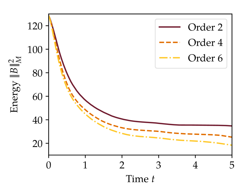
(a) Form 4 (split, central, split), energy.

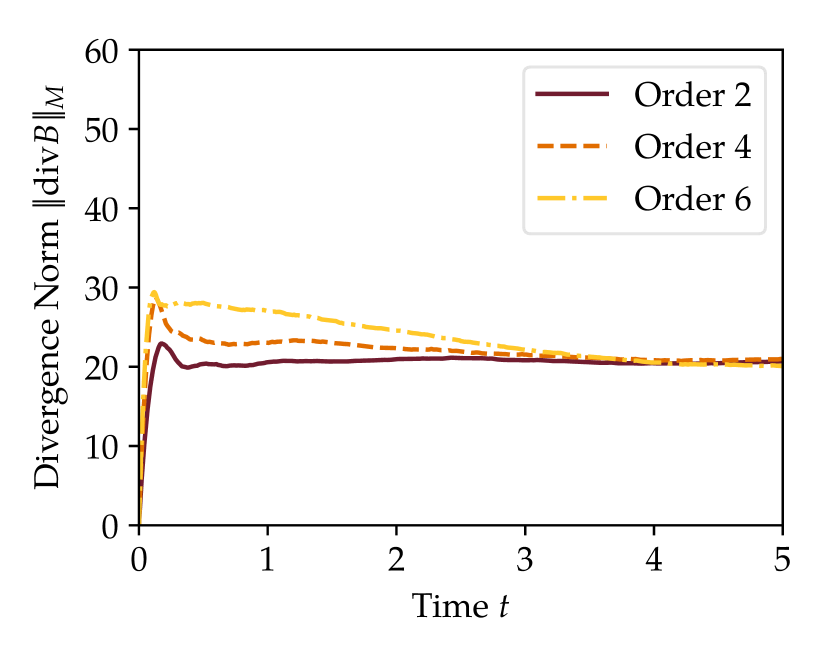
(b) Form 4 (split, central, split), $\mathinner{\!\left\lVert\operatorname{div}B\right\rVert}_{M}$.

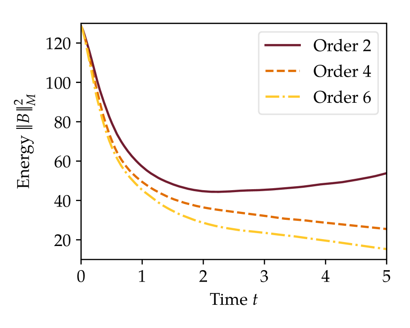
(c) Form 4 (product, central, split), energy.

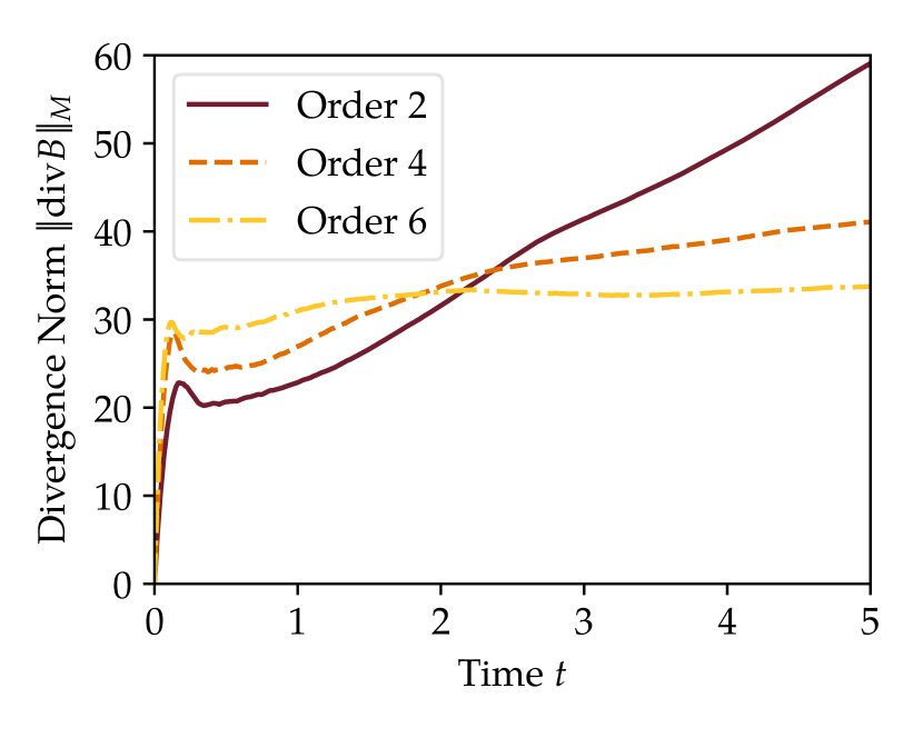
(d) Form 4 (product, central, split), $\mathinner{\!\left\lVert\operatorname{div}B\right\rVert}_{M}$.

Figure 1: Magnetic energy and divergence norms of numerical solutions of the nonlinear induction equation with Hall effect (65) using SBP operators of different order and two choices of forms given in Table 4.

As mentioned in Remark 3.2, the appearance of $u/2$ instead of $u$ in the proposed outflow boundary condition (83) might be irritating. However, simply replacing $u/2$ with $u$ results in schemes with worse performance concerning, e.g. the maximal stable time step. Indeed, maximal CFL numbers such that the numerical solutions do not blow up till the final time $T=1$ are given in Table 5. There, stable time steps are between two and three times as big for the proposed outflow boundary condition compared to the altered one. Note that no energy estimate has been obtained for the latter while the energy remains bounded if the proposed condition is used.

Table 5: Maximal CFL numbers such that numerical solutions of the nonlinear induction equation with Hall effect (65) using SBP operators of different orders and the choice 4 (central, central, central) do not blow up for $N=40$.

	Interior Order 2	Interior Order 4	Interior Order 6
$\frac{u}{2}-\frac{\nabla\times B}{\varrho}\dots$	$\mathrm{cfl}=1.9/N$	$\mathrm{cfl}=1.9/N$	$\mathrm{cfl}=1.5/N$
$u-\frac{\nabla\times B}{\varrho}\dots$	$\mathrm{cfl}=0.7/N$	$\mathrm{cfl}=0.6/N$	$\mathrm{cfl}=0.6/N$

5.5 Divergence Cleaning

In order to test the influence of the divergence cleaning schemes via different projection methods, setups of numerical experiments presented before will be used to compare properties of numerical solutions obtained with or without divergence cleaning.

The six parameter combinations of Table 4 have been used to compute numerical solutions for the test case described in section 5.2. The errors in $B$ and $\operatorname{div}B$ at the final time are given in Table 31 and Table 32 for the SBP operator with order of accuracy two and four, respectively. Both results have been obtained using $N=40$ nodes per space direction. Either no divergence cleaning procedure has been applied or the projection using

• the wide stencil operator with homogeneous Dirichlet boundary conditions (WS, D₀; section 4.3.1),

• the narrow stencil operator with zero Dirichlet boundary conditions (NS, D₀; section 4.3.3),

• the wide stencil operator and the least norm solution (WS, LN; section 4.3.4).

The absolute error threshold for the divergence has been set to $10^{-3}$ and up to $50$ iterations of the CG method have been performed after each time step.

The second order schemes using the same discretisation forms for $\partial_{j}(u_{i}B_{j})$ and $-\partial_{j}(u_{j}B_{i})$ perform already very well for this test case. Since the divergence norm is already negligible, the divergence cleaning procedure does not influence the results in Table 31.

For the other two parameter choices, the wide and narrow stencil discretisation of the Laplace operator with homogeneous Dirichlet boundary conditions yield results that are very similar to the ones without any divergence cleaning procedure at all. The wide stencil operator reduces the error a bit more. Contrary, the least norm solution yields a significant reduction of both the divergence errors and the magnetic energy. Nevertheless, the energy is still ca. 3–4 times larger than for the well-performing parameter combinations and the error in the magnetic field is of course not of the order of machine accuracy.

For the schemes with interior order of accuracy four, there is an initial divergence error of the magnetic field due to the projection of the initial condition onto the grid. Hence, the steady state can be left if divergence cleaning procedures area applied, as can be seen, e.g. in the first and fourth row of Table 32. As before, the least norm solutions performs better than the other divergence projection methods for this test case and the latter two ones perform similar. The trend of the results of the sixth order scheme is similar to the one of the fourth order scheme. Thus, these results are not presented here in greater detail.

Additional tests using the Hall term and outflow boundary conditions as in section 5.4 up to the final time $T=5$ have been performed. The results for the second and fourth order SBP operators are given in Table 33 and Table 34, respectively. As before, the wide stencil least norm approach is the only cleaning procedure resulting in a significant reduction of the divergence norm. The operators with homogeneous boundary conditions can give some stabilisation, e.g. for the (not recommended) choice 4 (central, zero, central) for the second order operator, cf. Table 33. For the other cases, they do not yield results that are significantly better than the ones without divergence cleaning procedure.

The results for the fourth order SBP operator are bit different. There, the wide stencil least norm approach results in a blow-up for three parameter combinations while the other approaches yield a blow-up of the numerical solution only for the choice 4 (central, zero, central). However, the divergence of the numerical solutions is reduced less than an order of magnitude by the operators using homogeneous Dirichlet boundary conditions.

Since the divergence cleaning via projection approach is relatively costly, it might be questionable whether it is worth the effort. In numerical experiments presented here, a desired stabilisation could also be provided by certain choices of the discrete forms given in Table 4. Of course, more detailed investigations studying the influence of the chosen error thresholds and maximum number of iterations could be carried out. However, the general results are not very sensitive to variations of these parameters and other means to control the divergence and stability of numerical solutions will be studied in the future.

6 Summary and Discussion

Building on the approach to stable problems in computational physics provided recently by [54], initial boundary value problems for the magnetic induction equation have been investigated at first at the continuous level. Using the common approach to add a non-conservative source term involving the divergence of the magnetic field, energy estimates have been obtained at first for the linear induction equation. By applying summation by parts operators and simultaneous approximation terms to impose boundary conditions weakly, these results have been transferred to the semidiscrete level. Thus, several different semidiscretisations of the induction equation have been shown to be energy stable (section 2). Additionally, the importance of boundary conditions for the divergence constraint has been demonstrated in section 2.6. Moreover, novel outflow boundary conditions for the nonlinear induction equation with Hall effect have been proposed, resulting in an energy estimate (section 3). Thereafter, divergence cleaning techniques using projections of the magnetic field have been studied. Using SBP operators and paying special attention to the boundaries, the energy of several known approaches has been investigated and a novel scheme with some improved properties has been proposed (section 4).

Finally, all schemes have been compared using several numerical test cases (section 5). In general, schemes using a nonconservative source term allow an energy estimate and perform better than the other ones in most test cases. While there might be some circumstances where the other schemes yield better results, it seems to be preferable to use methods allowing an energy estimate. However, having an energy estimate is not enough to predict the performance of a scheme on a finite grid. Indeed, the choice of the discrete form can influence the results considerably for certain test cases. In particular, preserving the anti-symmetry of $\nabla\times(u\times B)$ with respect to $u$ and $B$ can be very important, as has been demonstrated in numerical experiments. The novel outflow boundary condition for the nonlinear magnetic induction equation with Hall effect results in stable schemes and a decaying magnetic energy, as expected. Together with the other ingredients discussed and developed in this article, it will be tested in more demanding and realistic applications in the future.

The proposed schemes have been implemented in OpenCL and have been published as open source software [73] with Matlab interface via MatCL [29]. Further research will involve the optimisation of the implementation, other kinds of boundary conditions for the nonlinear induction equation with Hall effect, and other means to control divergence errors of the magnetic field.

Appendix A High-Order SBP Operators

Similarly to Example 2.4, there are higher order SBP operators. The following fourth order accurate SBP operators are given in [48]. The lower right corner can be obtained from the upper right corner via $D_{N+1-i,N+1-j}=-D_{i,j}$.

$$\begin{gathered}D=\frac{1}{\Delta x}\begin{pmatrix}\nicefrac{{-24}}{{17}}&\nicefrac{{59}}{{34}}&\nicefrac{{-4}}{{17}}&\nicefrac{{-3}}{{34}}\\ \nicefrac{{-1}}{{2}}&0&\nicefrac{{1}}{{2}}\\ \nicefrac{{4}}{{43}}&\nicefrac{{-59}}{{86}}&0&\nicefrac{{59}}{{86}}&\nicefrac{{-4}}{{43}}\\ \nicefrac{{3}}{{98}}&0&\nicefrac{{-59}}{{98}}&0&\nicefrac{{32}}{{49}}&\nicefrac{{-4}}{{49}}\\ &&\nicefrac{{1}}{{12}}&\nicefrac{{-2}}{{3}}&0&\nicefrac{{2}}{{3}}&\nicefrac{{-1}}{{12}}\\ &&&\ddots&\ddots&\ddots&\ddots&\ddots\\ \end{pmatrix},\\ M=\Delta x\operatorname{diag}\left(\frac{17}{48},\frac{59}{48},\frac{43}{48},\frac{49}{48},1,\dots,1,\frac{49}{48},\frac{43}{48},\frac{59}{48},\frac{17}{48}\right).\end{gathered}$$ (124)

Using the approach of section 4.3.4 for divergence cleaning, the adjoint operator $D^{*}$ and $DD^{*}$ have to be used. Similarly to Example 4.11, they are

$$D^{*}=M^{-1}D^{T}M=-D+M^{-1}E=\frac{1}{\Delta x}\begin{pmatrix}\nicefrac{{-24}}{{17}}&\nicefrac{{-59}}{{34}}&\nicefrac{{4}}{{17}}&\nicefrac{{3}}{{34}}\\ \nicefrac{{1}}{{2}}&0&\nicefrac{{-1}}{{2}}\\ \nicefrac{{-4}}{{43}}&\nicefrac{{59}}{{86}}&0&\nicefrac{{-59}}{{86}}&\nicefrac{{4}}{{43}}\\ \nicefrac{{-3}}{{98}}&0&\nicefrac{{59}}{{98}}&0&\nicefrac{{-32}}{{49}}&\nicefrac{{4}}{{49}}\\ &&\nicefrac{{-1}}{{12}}&\nicefrac{{2}}{{3}}&0&\nicefrac{{-2}}{{3}}&\nicefrac{{1}}{{12}}\\ &&&\ddots&\ddots&\ddots&\ddots&\ddots\\ \end{pmatrix}$$ (125)

and

$$\Delta x^{2}\;DD^{*}=\\ \setcounter{MaxMatrixCols}{11}\begin{pmatrix}\nicefrac{{1756935}}{{608923}}&\nicefrac{{28438}}{{12427}}&\nicefrac{{-17743}}{{14161}}&\nicefrac{{458}}{{12427}}&\nicefrac{{1280}}{{35819}}&\nicefrac{{-6}}{{833}}\\ \nicefrac{{482}}{{731}}&\nicefrac{{885}}{{731}}&\nicefrac{{-2}}{{17}}&\nicefrac{{-283}}{{731}}&\nicefrac{{2}}{{43}}\\ \nicefrac{{-17743}}{{35819}}&\nicefrac{{-118}}{{731}}&\nicefrac{{84428}}{{107457}}&\nicefrac{{-118}}{{2193}}&\nicefrac{{-944}}{{2107}}&\nicefrac{{746}}{{6321}}&\nicefrac{{-1}}{{129}}\\ \nicefrac{{458}}{{35819}}&\nicefrac{{-16697}}{{35819}}&\nicefrac{{-118}}{{2499}}&\nicefrac{{92188}}{{107457}}&\nicefrac{{-698}}{{6321}}&\nicefrac{{-64}}{{147}}&\nicefrac{{16}}{{147}}&\nicefrac{{-1}}{{147}}\\ \nicefrac{{80}}{{6321}}&\nicefrac{{59}}{{1032}}&\nicefrac{{-59}}{{147}}&\nicefrac{{-349}}{{3096}}&\nicefrac{{271403}}{{303408}}&\nicefrac{{-97}}{{882}}&\nicefrac{{-4}}{{9}}&\nicefrac{{1}}{{9}}&\nicefrac{{-1}}{{144}}\\ \nicefrac{{-1}}{{392}}&0&\nicefrac{{373}}{{3528}}&\nicefrac{{-4}}{{9}}&\nicefrac{{-97}}{{882}}&\nicefrac{{2123}}{{2352}}&\nicefrac{{-1}}{{9}}&\nicefrac{{-4}}{{9}}&\nicefrac{{1}}{{9}}&\nicefrac{{-1}}{{144}}\\ 0&0&\nicefrac{{-1}}{{144}}&\nicefrac{{1}}{{9}}&\nicefrac{{-4}}{{9}}&\nicefrac{{-1}}{{9}}&\nicefrac{{65}}{{72}}&\nicefrac{{-1}}{{9}}&\nicefrac{{-4}}{{9}}&\nicefrac{{1}}{{9}}&\nicefrac{{-1}}{{144}}\\ &&&\ddots&\ddots&\ddots&\ddots&\ddots&\ddots&\ddots&\ddots\end{pmatrix}.$$ (126)

This operator is symmetric and positive semidefinite. Coefficients for the derivative operators with interior order of accuracy six can be found in [48]. All coefficients can also be found in [73].

Appendix B Results of Numerical Experiments

Here, additional data from numerical experiments described in section 5 are given.

Table 6: Errors and divergence norms of numerical solutions of the linear induction equation (2) with analytical solution (118) using $N=40$ nodes per direction and the fourth order SBP operator.

$\partial_{j}(u_{i}B_{j})$	source term	$-\partial_{j}(u_{j}B_{i})$	$\varepsilon_{B}$	$\varepsilon_{\operatorname{div}B}$
product	zero	product	1.10e+06	9.18e+06
product	zero	split	1.10e+06	9.18e+06
product	zero	central	1.10e+06	9.18e+06
product	split	product	2.04e-02	8.42e-02
product	split	split	2.04e-02	8.42e-02
product	split	central	2.04e-02	8.42e-02
product	central	product	2.01e-02	5.66e-02
product	central	split	2.01e-02	5.66e-02
product	central	central	2.01e-02	5.66e-02
split	zero	product	2.26e+02	1.43e+03
split	zero	split	2.26e+02	1.43e+03
split	zero	central	2.26e+02	1.43e+03
split	split	product	2.01e-02	5.66e-02
split	split	split	2.01e-02	5.66e-02
split	split	central	2.01e-02	5.66e-02
split	central	product	1.99e-02	2.86e-02
split	central	split	1.99e-02	2.86e-02
split	central	central	1.99e-02	2.86e-02
central	zero	product	1.98e-02	4.87e-03
central	zero	split	1.98e-02	4.87e-03
central	zero	central	1.98e-02	4.87e-03
central	split	product	1.99e-02	2.86e-02
central	split	split	1.99e-02	2.86e-02
central	split	central	1.99e-02	2.86e-02
central	central	product	1.98e-02	3.04e-03
central	central	split	1.98e-02	3.04e-03
central	central	central	1.98e-02	3.04e-03

Table 7: Results of convergence experiments for the linear induction equation (2) with analytical solution (118), SBP operators of different order, and the choice of discrete forms as in 4 (central, zero, central).

	Interior Order $2$					Interior Order $4$					Interior Order $6$
$N$	$\varepsilon_{B}$	EOC	$\varepsilon_{\operatorname{div}B}$	EOC	Runtime	$\varepsilon_{B}$	EOC	$\varepsilon_{\operatorname{div}B}$	EOC	Runtime	$\varepsilon_{B}$	EOC	$\varepsilon_{\operatorname{div}B}$	EOC	Runtime
$40$	1.72e-01		2.77e-02		7.18e-01	1.98e-02		4.87e-03		1.02e+00	3.79e-03		8.51e-03		1.34e+00
$80$	5.37e-02	1.68	7.14e-03	1.95	1.10e+01	1.27e-03	3.96	5.82e-04	3.07	1.62e+01	1.18e-04	5.01	6.87e-04	3.63	2.36e+01
$160$	1.36e-02	1.98	2.02e-03	1.82	1.69e+02	7.88e-05	4.01	8.37e-05	2.80	3.03e+02	4.63e-06	4.67	5.01e-05	3.78	4.20e+02
$320$	3.39e-03	2.01	6.23e-04	1.70	2.92e+03	4.90e-06	4.01	1.35e-05	2.63	5.69e+03	2.39e-07	4.27	3.88e-06	3.69	9.47e+03

Table 8: Results of convergence experiments for the linear induction equation (2) with analytical solution (118), SBP operators of different order, and the choice of discrete forms as in 4 (central, central, central).

	Interior Order $2$					Interior Order $4$					Interior Order $6$
$N$	$\varepsilon_{B}$	EOC	$\varepsilon_{\operatorname{div}B}$	EOC	Runtime	$\varepsilon_{B}$	EOC	$\varepsilon_{\operatorname{div}B}$	EOC	Runtime	$\varepsilon_{B}$	EOC	$\varepsilon_{\operatorname{div}B}$	EOC	Runtime
$40$	1.72e-01		3.74e-02		7.31e-01	1.98e-02		3.04e-03		1.06e+00	3.70e-03		9.83e-03		1.45e+00
$80$	5.37e-02	1.68	7.13e-03	2.39	1.13e+01	1.27e-03	3.96	2.80e-04	3.44	1.67e+01	1.13e-04	5.04	6.56e-04	3.90	2.48e+01
$160$	1.36e-02	1.98	1.99e-03	1.84	1.93e+02	7.89e-05	4.01	3.81e-05	2.88	3.21e+02	4.91e-06	4.52	4.40e-05	3.90	4.40e+02
$320$	3.39e-03	2.01	5.97e-04	1.73	2.95e+03	4.93e-06	4.00	5.42e-06	2.81	5.75e+03	2.68e-07	4.19	3.33e-06	3.73	8.74e+03

Table 9: Results of convergence experiments for the linear induction equation (2) with analytical solution (118), SBP operators of different order, and the choice of discrete forms as in 4 (split, central, split).

	Interior Order $2$					Interior Order $4$					Interior Order $6$
$N$	$\varepsilon_{B}$	EOC	$\varepsilon_{\operatorname{div}B}$	EOC	Runtime	$\varepsilon_{B}$	EOC	$\varepsilon_{\operatorname{div}B}$	EOC	Runtime	$\varepsilon_{B}$	EOC	$\varepsilon_{\operatorname{div}B}$	EOC	Runtime
$40$	1.75e-01		2.99e-01		7.42e-01	1.99e-02		2.86e-02		1.12e+00	3.30e-03		2.03e-02		1.55e+00
$80$	5.41e-02	1.69	7.72e-02	1.95	1.14e+01	1.28e-03	3.96	1.82e-03	3.97	1.74e+01	8.86e-05	5.22	1.20e-03	4.08	2.66e+01
$160$	1.37e-02	1.98	1.94e-02	2.00	1.79e+02	7.91e-05	4.01	1.17e-04	3.96	3.15e+02	3.73e-06	4.57	6.73e-05	4.15	4.69e+02
$320$	3.41e-03	2.01	4.85e-03	2.00	3.12e+03	4.93e-06	4.00	8.82e-06	3.73	5.83e+03	2.04e-07	4.20	5.02e-06	3.74	9.42e+03

Table 10: Results of convergence experiments for the linear induction equation (2) with analytical solution (118), SBP operators of different order, and the choice of discrete forms as in 4 (product, central, product).

	Interior Order $2$					Interior Order $4$					Interior Order $6$
$N$	$\varepsilon_{B}$	EOC	$\varepsilon_{\operatorname{div}B}$	EOC	Runtime	$\varepsilon_{B}$	EOC	$\varepsilon_{\operatorname{div}B}$	EOC	Runtime	$\varepsilon_{B}$	EOC	$\varepsilon_{\operatorname{div}B}$	EOC	Runtime
$40$	1.74e-01		5.69e-01		7.38e-01	2.01e-02		5.66e-02		1.07e+00	3.08e-03		2.09e-02		1.50e+00
$80$	5.49e-02	1.66	1.53e-01	1.89	1.14e+01	1.29e-03	3.96	3.61e-03	3.97	1.72e+01	6.86e-05	5.49	1.01e-03	4.38	2.56e+01
$160$	1.39e-02	1.98	3.85e-02	1.99	1.80e+02	8.01e-05	4.01	2.25e-04	4.00	3.02e+02	2.84e-06	4.59	4.70e-05	4.42	4.53e+02
$320$	3.47e-03	2.01	9.63e-03	2.00	3.09e+03	4.98e-06	4.01	1.46e-05	3.94	5.73e+03	1.62e-07	4.13	2.86e-06	4.04	9.31e+03

Table 11: Results of convergence experiments for the linear induction equation (2) with analytical solution (118), SBP operators of different order, and the choice of discrete forms as in 4 (product, central, split).

	Interior Order $2$					Interior Order $4$					Interior Order $6$
$N$	$\varepsilon_{B}$	EOC	$\varepsilon_{\operatorname{div}B}$	EOC	Runtime	$\varepsilon_{B}$	EOC	$\varepsilon_{\operatorname{div}B}$	EOC	Runtime	$\varepsilon_{B}$	EOC	$\varepsilon_{\operatorname{div}B}$	EOC	Runtime
$40$	1.74e-01		5.69e-01		7.59e-01	2.01e-02		5.66e-02		1.10e+00	3.08e-03		2.09e-02		1.52e+00
$80$	5.49e-02	1.66	1.53e-01	1.89	1.16e+01	1.29e-03	3.96	3.61e-03	3.97	1.73e+01	6.86e-05	5.49	1.01e-03	4.38	2.59e+01
$160$	1.39e-02	1.98	3.85e-02	1.99	1.87e+02	8.01e-05	4.01	2.25e-04	4.00	3.16e+02	2.84e-06	4.59	4.70e-05	4.42	4.39e+02
$320$	3.47e-03	2.01	9.63e-03	2.00	3.03e+03	4.98e-06	4.01	1.46e-05	3.94	5.93e+03	1.62e-07	4.13	2.86e-06	4.04	7.55e+03

Table 12: Results of convergence experiments for the linear induction equation (2) with analytical solution (118), SBP operators of different order, and the choice of discrete forms as in 4 (product, central, central).

	Interior Order $2$					Interior Order $4$					Interior Order $6$
$N$	$\varepsilon_{B}$	EOC	$\varepsilon_{\operatorname{div}B}$	EOC	Runtime	$\varepsilon_{B}$	EOC	$\varepsilon_{\operatorname{div}B}$	EOC	Runtime	$\varepsilon_{B}$	EOC	$\varepsilon_{\operatorname{div}B}$	EOC	Runtime
$40$	1.74e-01		5.69e-01		7.39e-01	2.01e-02		5.66e-02		1.08e+00	3.08e-03		2.09e-02		1.47e+00
$80$	5.49e-02	1.66	1.53e-01	1.89	1.14e+01	1.29e-03	3.96	3.61e-03	3.97	1.72e+01	6.86e-05	5.49	1.01e-03	4.38	2.54e+01
$160$	1.39e-02	1.98	3.85e-02	1.99	1.78e+02	8.01e-05	4.01	2.25e-04	4.00	3.20e+02	2.84e-06	4.59	4.70e-05	4.42	4.41e+02
$320$	3.47e-03	2.01	9.63e-03	2.00	2.81e+03	4.98e-06	4.01	1.46e-05	3.94	5.82e+03	1.62e-07	4.13	2.86e-06	4.04	8.02e+03

Table 13: Errors and divergence norms of numerical solutions of the linear induction equation (2) with analytical solution (120) using $N=40$ nodes per direction and the fourth order SBP operator.

$\partial_{j}(u_{i}B_{j})$	source term	$-\partial_{j}(u_{j}B_{i})$	$\varepsilon_{B}$	$\varepsilon_{\operatorname{div}B}$
product	zero	product	1.55e-12	1.77e-03
product	zero	split	9.32e+03	4.88e+05
product	zero	central	4.63e+09	1.98e+11
product	split	product	2.74e+02	8.81e+02
product	split	split	1.39e+04	9.19e+05
product	split	central	3.07e+09	2.30e+11
product	central	product	6.65e-02	5.66e-01
product	central	split	1.33e+00	4.85e+00
product	central	central	1.64e+03	1.09e+05
split	zero	product	2.88e+05	4.90e+06
split	zero	split	2.98e-17	1.77e-03
split	zero	central	1.44e+03	7.53e+04
split	split	product	6.65e-02	5.66e-01
split	split	split	1.33e+00	4.85e+00
split	split	central	1.64e+03	1.09e+05
split	central	product	3.80e+01	1.17e+02
split	central	split	3.50e-03	2.93e-02
split	central	central	3.75e-01	1.37e+00
central	zero	product	4.03e+07	1.11e+09
central	zero	split	3.20e+01	7.43e+02
central	zero	central	0.00e+00	1.77e-03
central	split	product	3.80e+01	1.17e+02
central	split	split	3.50e-03	2.93e-02
central	split	central	3.75e-01	1.37e+00
central	central	product	2.77e+04	5.72e+05
central	central	split	2.54e-01	1.21e+00
central	central	central	4.09e-03	3.68e-02

Table 14: Results of convergence experiments for the linear induction equation (2) with analytical solution (120), SBP operators of different order, and the choice of discrete forms as in 4 (central, zero, central).

	Interior Order $2$					Interior Order $4$					Interior Order $6$
$N$	$\varepsilon_{B}$	EOC	$\varepsilon_{\operatorname{div}B}$	EOC	Runtime	$\varepsilon_{B}$	EOC	$\varepsilon_{\operatorname{div}B}$	EOC	Runtime	$\varepsilon_{B}$	EOC	$\varepsilon_{\operatorname{div}B}$	EOC	Runtime
$40$	1.87e-30		4.10e-15		6.17e-01	2.73e-30		1.77e-03		8.02e-01	4.33e-30		7.77e-05		1.11e+00
$80$	8.13e-31	1.20	7.28e-15	-0.83	9.33e+00	9.12e-31	1.58	3.04e-04	2.54	1.33e+01	1.21e-30	1.84	3.26e-06	4.57	2.02e+01
$160$	1.18e-30	-0.53	9.24e-15	-0.34	1.53e+02	1.35e-30	-0.56	5.30e-05	2.52	2.70e+02	1.56e-30	-0.37	1.40e-07	4.54	3.66e+02
$320$	2.11e-29	-4.17	2.24e-14	-1.28	2.49e+03	2.58e-29	-4.26	9.29e-06	2.51	4.55e+03	2.76e-29	-4.14	6.12e-09	4.52	8.47e+03

Table 15: Results of convergence experiments for the linear induction equation (2) with analytical solution (120), SBP operators of different order, and the choice of discrete forms as in 4 (central, central, central).

	Interior Order $2$					Interior Order $4$					Interior Order $6$
$N$	$\varepsilon_{B}$	EOC	$\varepsilon_{\operatorname{div}B}$	EOC	Runtime	$\varepsilon_{B}$	EOC	$\varepsilon_{\operatorname{div}B}$	EOC	Runtime	$\varepsilon_{B}$	EOC	$\varepsilon_{\operatorname{div}B}$	EOC	Runtime
$40$	9.74e-16		1.36e-14		6.08e-01	4.09e-03		3.68e-02		8.50e-01	3.55e-04		4.86e-03		1.20e+00
$80$	1.49e-15	-0.61	5.34e-14	-1.98	9.41e+00	6.02e-04	2.76	1.41e-02	1.39	1.39e+01	1.69e-05	4.39	3.42e-04	3.83	2.12e+01
$160$	1.57e-15	-0.08	1.55e-13	-1.54	1.43e+02	6.55e-05	3.20	5.46e-03	1.37	2.74e+02	5.40e-07	4.97	2.85e-05	3.59	3.81e+02
$320$	5.13e-15	-1.70	9.31e-13	-2.59	2.60e+03	7.71e-06	3.09	1.88e-03	1.54	4.87e+03	1.30e-08	5.38	2.45e-06	3.54	8.58e+03

Table 16: Results of convergence experiments for the linear induction equation (2) with analytical solution (120), SBP operators of different order, and the choice of discrete forms as in 4 (split, central, split).

	Interior Order $2$					Interior Order $4$					Interior Order $6$
$N$	$\varepsilon_{B}$	EOC	$\varepsilon_{\operatorname{div}B}$	EOC	Runtime	$\varepsilon_{B}$	EOC	$\varepsilon_{\operatorname{div}B}$	EOC	Runtime	$\varepsilon_{B}$	EOC	$\varepsilon_{\operatorname{div}B}$	EOC	Runtime
$40$	1.48e-15		2.28e-14		5.86e-01	3.50e-03		2.93e-02		9.10e-01	1.17e-04		1.80e-03		1.27e+00
$80$	2.26e-15	-0.61	7.59e-14	-1.74	9.90e+00	5.27e-04	2.73	6.76e-03	2.12	1.47e+01	6.10e-06	4.27	1.14e-04	3.98	2.26e+01
$160$	2.07e-15	0.12	1.91e-13	-1.33	1.51e+02	6.59e-05	3.00	1.45e-03	2.22	2.84e+02	3.02e-07	4.33	7.23e-06	3.98	4.08e+02
$320$	6.84e-15	-1.72	1.10e-12	-2.52	2.57e+03	8.96e-06	2.88	3.08e-04	2.23	5.38e+03	1.19e-08	4.66	4.54e-07	3.99	8.90e+03

Table 17: Results of convergence experiments for the linear induction equation (2) with analytical solution (120), SBP operators of different order, and the choice of discrete forms as in 4 (product, central, product).

	Interior Order $2$					Interior Order $4$					Interior Order $6$
$N$	$\varepsilon_{B}$	EOC	$\varepsilon_{\operatorname{div}B}$	EOC	Runtime	$\varepsilon_{B}$	EOC	$\varepsilon_{\operatorname{div}B}$	EOC	Runtime	$\varepsilon_{B}$	EOC	$\varepsilon_{\operatorname{div}B}$	EOC	Runtime
$40$	7.35e-14		8.21e-13		6.21e-01	6.65e-02		5.66e-01		8.75e-01	1.59e-03		1.41e-02		1.25e+00
$80$	1.86e-13	-1.34	1.28e-12	-0.65	9.76e+00	1.01e-02	2.72	1.68e-01	1.75	1.45e+01	5.99e-05	4.73	8.55e-04	4.04	2.17e+01
$160$	3.89e-13	-1.07	3.09e-12	-1.27	1.59e+02	1.58e-03	2.67	5.48e-02	1.62	2.78e+02	2.76e-06	4.44	5.92e-05	3.85	3.91e+02
$320$	6.36e-13	-0.71	1.34e-11	-2.11	2.62e+03	2.83e-04	2.48	1.75e-02	1.65	5.08e+03	1.37e-07	4.33	4.67e-06	3.66	8.55e+03

Table 18: Results of convergence experiments for the linear induction equation (2) with analytical solution (120), SBP operators of different order, and the choice of discrete forms as in 4 (product, central, split).

	Interior Order $2$					Interior Order $4$					Interior Order $6$
$N$	$\varepsilon_{B}$	EOC	$\varepsilon_{\operatorname{div}B}$	EOC	Runtime	$\varepsilon_{B}$	EOC	$\varepsilon_{\operatorname{div}B}$	EOC	Runtime	$\varepsilon_{B}$	EOC	$\varepsilon_{\operatorname{div}B}$	EOC	Runtime
$40$	8.49e+01		2.86e+02		6.41e-01	1.33e+00		4.85e+00		8.98e-01	1.73e+00		1.23e+01		1.30e+00
$80$	4.05e+01	1.07	1.68e+02	0.77	9.45e+00	1.61e-01	3.04	6.97e-01	2.80	1.44e+01	2.44e-01	2.82	1.22e+00	3.33	2.17e+01
$160$	1.85e+01	1.13	1.08e+02	0.63	1.49e+02	1.95e-02	3.04	1.83e-01	1.93	2.80e+02	3.00e-02	3.02	1.02e-01	3.58	4.02e+02
$320$	8.31e+00	1.16	7.43e+01	0.54	2.62e+03	2.30e-03	3.09	5.61e-02	1.71	5.22e+03	3.61e-03	3.06	7.30e-03	3.80	8.99e+03

Table 19: Results of convergence experiments for the linear induction equation (2) with analytical solution (120), SBP operators of different order, and the choice of discrete forms as in 4 (product, central, central).

	Interior Order $2$					Interior Order $4$					Interior Order $6$
$N$	$\varepsilon_{B}$	EOC	$\varepsilon_{\operatorname{div}B}$	EOC	Runtime	$\varepsilon_{B}$	EOC	$\varepsilon_{\operatorname{div}B}$	EOC	Runtime	$\varepsilon_{B}$	EOC	$\varepsilon_{\operatorname{div}B}$	EOC	Runtime
$40$	3.52e+04		1.68e+06		6.19e-01	1.64e+03		1.09e+05		8.57e-01	8.33e+03		6.43e+05		1.22e+00
$80$	2.36e+04	0.58	2.29e+06	-0.44	9.60e+00	2.61e+02	2.65	3.50e+04	1.63	1.40e+01	1.44e+03	2.53	2.25e+05	1.52	2.10e+01
$160$	1.51e+04	0.65	2.93e+06	-0.36	1.53e+02	4.06e+01	2.68	1.10e+04	1.68	2.75e+02	2.30e+02	2.64	7.24e+04	1.64	4.09e+02
$320$	8.93e+03	0.75	3.49e+06	-0.25	2.63e+03	5.85e+00	2.79	3.17e+03	1.79	5.16e+03	3.38e+01	2.77	2.13e+04	1.76	8.61e+03

Table 20: Results of convergence experiments for the nonlinear induction equation (65) with analytical solution (121), SBP operators of different order, and the choice of discrete forms as in 4 (central, zero, central).

	Interior Order $2$					Interior Order $4$					Interior Order $6$
$N$	$\varepsilon_{B}$	EOC	$\varepsilon_{\operatorname{div}B}$	EOC	Runtime	$\varepsilon_{B}$	EOC	$\varepsilon_{\operatorname{div}B}$	EOC	Runtime	$\varepsilon_{B}$	EOC	$\varepsilon_{\operatorname{div}B}$	EOC	Runtime
$40$	2.02e-02		2.55e-13		5.59e+00	9.98e-05		3.44e-13		6.85e+00	5.27e-07		3.94e-13		8.26e+00
$60$	9.00e-03	1.99	5.76e-13	-2.01	4.18e+01	1.97e-05	4.00	7.78e-13	-2.01	5.34e+01	4.64e-08	5.99	8.83e-13	-1.99	6.65e+01
$80$	5.07e-03	2.00	1.02e-12	-2.00	1.97e+02	6.25e-06	4.00	1.38e-12	-1.99	2.26e+02	8.26e-09	6.00	1.57e-12	-2.00	3.16e+02
$100$	3.24e-03	2.00	1.61e-12	-2.02	5.70e+02	2.56e-06	4.00	2.15e-12	-2.00	7.69e+02	2.17e-09	6.00	2.46e-12	-2.01	9.57e+02

Table 21: Results of convergence experiments for the nonlinear induction equation (65) with analytical solution (121), SBP operators of different order, and the choice of discrete forms as in 4 (central, central, central).

	Interior Order $2$					Interior Order $4$					Interior Order $6$
$N$	$\varepsilon_{B}$	EOC	$\varepsilon_{\operatorname{div}B}$	EOC	Runtime	$\varepsilon_{B}$	EOC	$\varepsilon_{\operatorname{div}B}$	EOC	Runtime	$\varepsilon_{B}$	EOC	$\varepsilon_{\operatorname{div}B}$	EOC	Runtime
$40$	2.02e-02		2.56e-13		5.80e+00	9.98e-05		3.47e-13		6.83e+00	5.27e-07		3.93e-13		8.28e+00
$60$	9.00e-03	1.99	5.76e-13	-2.00	4.39e+01	1.97e-05	4.00	7.76e-13	-1.99	5.19e+01	4.64e-08	5.99	8.82e-13	-1.99	6.61e+01
$80$	5.07e-03	2.00	1.03e-12	-2.02	1.94e+02	6.25e-06	4.00	1.38e-12	-2.00	2.28e+02	8.26e-09	6.00	1.58e-12	-2.02	3.14e+02
$100$	3.24e-03	2.00	1.61e-12	-2.00	5.74e+02	2.56e-06	4.00	2.16e-12	-2.00	7.48e+02	2.17e-09	6.00	2.46e-12	-1.99	9.48e+02

Table 22: Results of convergence experiments for the nonlinear induction equation (65) with analytical solution (121), SBP operators of different order, and the choice of discrete forms as in 4 (split, central, split).

	Interior Order $2$					Interior Order $4$					Interior Order $6$
$N$	$\varepsilon_{B}$	EOC	$\varepsilon_{\operatorname{div}B}$	EOC	Runtime	$\varepsilon_{B}$	EOC	$\varepsilon_{\operatorname{div}B}$	EOC	Runtime	$\varepsilon_{B}$	EOC	$\varepsilon_{\operatorname{div}B}$	EOC	Runtime
$40$	2.02e-02		1.48e-03		5.82e+00	9.98e-05		1.02e-05		7.19e+00	5.27e-07		6.34e-08		9.03e+00
$60$	9.00e-03	2.00	5.30e-04	2.53	4.41e+01	1.98e-05	4.00	1.71e-06	4.40	5.75e+01	4.64e-08	5.99	4.78e-09	6.38	7.50e+01
$80$	5.07e-03	2.00	2.66e-04	2.40	1.87e+02	6.25e-06	4.00	4.76e-07	4.44	2.44e+02	8.26e-09	6.00	7.55e-10	6.41	3.40e+02
$100$	3.24e-03	2.00	1.63e-04	2.21	5.65e+02	2.56e-06	4.00	1.82e-07	4.32	8.63e+02	2.17e-09	6.00	1.88e-10	6.24	1.04e+03

Table 23: Results of convergence experiments for the nonlinear induction equation (65) with analytical solution (121), SBP operators of different order, and the choice of discrete forms as in 4 (product, central, product).

	Interior Order $2$					Interior Order $4$					Interior Order $6$
$N$	$\varepsilon_{B}$	EOC	$\varepsilon_{\operatorname{div}B}$	EOC	Runtime	$\varepsilon_{B}$	EOC	$\varepsilon_{\operatorname{div}B}$	EOC	Runtime	$\varepsilon_{B}$	EOC	$\varepsilon_{\operatorname{div}B}$	EOC	Runtime
$40$	2.03e-02		3.03e-03		5.81e+00	9.99e-05		2.05e-05		6.94e+00	5.27e-07		1.30e-07		8.66e+00
$60$	9.01e-03	2.00	1.07e-03	2.56	4.37e+01	1.98e-05	4.00	3.42e-06	4.42	5.24e+01	4.64e-08	5.99	9.72e-09	6.39	6.90e+01
$80$	5.07e-03	2.00	5.39e-04	2.40	1.93e+02	6.25e-06	4.00	9.58e-07	4.43	2.45e+02	8.26e-09	6.00	1.55e-09	6.38	3.03e+02
$100$	3.25e-03	2.00	3.29e-04	2.21	5.63e+02	2.56e-06	4.00	3.68e-07	4.29	7.64e+02	2.17e-09	6.00	3.87e-10	6.21	9.93e+02

Table 24: Results of convergence experiments for the nonlinear induction equation (65) with analytical solution (121), SBP operators of different order, and the choice of discrete forms as in 4 (product, central, split).

	Interior Order $2$					Interior Order $4$					Interior Order $6$
$N$	$\varepsilon_{B}$	EOC	$\varepsilon_{\operatorname{div}B}$	EOC	Runtime	$\varepsilon_{B}$	EOC	$\varepsilon_{\operatorname{div}B}$	EOC	Runtime	$\varepsilon_{B}$	EOC	$\varepsilon_{\operatorname{div}B}$	EOC	Runtime
$40$	2.03e-02		3.03e-03		5.87e+00	9.99e-05		2.05e-05		7.30e+00	5.27e-07		1.30e-07		9.35e+00
$60$	9.01e-03	2.00	1.07e-03	2.56	4.28e+01	1.98e-05	4.00	3.42e-06	4.42	5.53e+01	4.64e-08	5.99	9.72e-09	6.39	7.23e+01
$80$	5.07e-03	2.00	5.39e-04	2.40	1.91e+02	6.25e-06	4.00	9.58e-07	4.43	2.59e+02	8.26e-09	6.00	1.55e-09	6.38	3.22e+02
$100$	3.25e-03	2.00	3.29e-04	2.21	5.83e+02	2.56e-06	4.00	3.68e-07	4.29	8.29e+02	2.17e-09	6.00	3.87e-10	6.21	1.06e+03

Table 25: Results of convergence experiments for the nonlinear induction equation (65) with analytical solution (121), SBP operators of different order, and the choice of discrete forms as in 4 (product, central, central).

	Interior Order $2$					Interior Order $4$					Interior Order $6$
$N$	$\varepsilon_{B}$	EOC	$\varepsilon_{\operatorname{div}B}$	EOC	Runtime	$\varepsilon_{B}$	EOC	$\varepsilon_{\operatorname{div}B}$	EOC	Runtime	$\varepsilon_{B}$	EOC	$\varepsilon_{\operatorname{div}B}$	EOC	Runtime
$40$	2.03e-02		3.03e-03		5.73e+00	9.99e-05		2.05e-05		6.99e+00	5.27e-07		1.30e-07		8.36e+00
$60$	9.01e-03	2.00	1.07e-03	2.56	4.28e+01	1.98e-05	4.00	3.42e-06	4.42	5.25e+01	4.64e-08	5.99	9.72e-09	6.39	6.49e+01
$80$	5.07e-03	2.00	5.39e-04	2.40	1.90e+02	6.25e-06	4.00	9.58e-07	4.43	2.50e+02	8.26e-09	6.00	1.55e-09	6.38	3.08e+02
$100$	3.25e-03	2.00	3.29e-04	2.21	5.85e+02	2.56e-06	4.00	3.68e-07	4.29	7.81e+02	2.17e-09	6.00	3.87e-10	6.21	9.32e+02

Table 26: Results of numerical experiments for the nonlinear induction equation (65) using SBP operators of different order and the choice of discrete forms as in 4 (central, central, central).

	Interior Order $2$			Interior Order $4$			Interior Order $6$
$N$	$\mathinner{\!\left\lVert B\right\rVert}_{M}^{2}$	$\mathinner{\!\left\lVert D_{i}B_{i}\right\rVert}_{M}$	Runtime	$\mathinner{\!\left\lVert B\right\rVert}_{M}^{2}$	$\mathinner{\!\left\lVert D_{i}B_{i}\right\rVert}_{M}$	Runtime	$\mathinner{\!\left\lVert B\right\rVert}_{M}^{2}$	$\mathinner{\!\left\lVert D_{i}B_{i}\right\rVert}_{M}$	Runtime
$40$	5.68e+01	2.01e+01	3.71e+00	4.88e+01	2.23e+01	5.36e+00	4.51e+01	2.64e+01	7.36e+00
$80$	4.61e+01	2.79e+01	6.88e+01	4.23e+01	3.13e+01	1.16e+02	4.03e+01	3.67e+01	1.70e+02

Table 27: Results of numerical experiments for the nonlinear induction equation (65) using SBP operators of different order and the choice of discrete forms as in 4 (split, central, split).

	Interior Order $2$			Interior Order $4$			Interior Order $6$
$N$	$\mathinner{\!\left\lVert B\right\rVert}_{M}^{2}$	$\mathinner{\!\left\lVert D_{i}B_{i}\right\rVert}_{M}$	Runtime	$\mathinner{\!\left\lVert B\right\rVert}_{M}^{2}$	$\mathinner{\!\left\lVert D_{i}B_{i}\right\rVert}_{M}$	Runtime	$\mathinner{\!\left\lVert B\right\rVert}_{M}^{2}$	$\mathinner{\!\left\lVert D_{i}B_{i}\right\rVert}_{M}$	Runtime
$40$	5.66e+01	2.05e+01	3.48e+00	4.86e+01	2.31e+01	5.00e+00	4.48e+01	2.69e+01	7.15e+00
$80$	4.60e+01	2.88e+01	6.55e+01	4.21e+01	3.28e+01	1.08e+02	4.04e+01	3.78e+01	1.66e+02

Table 28: Results of numerical experiments for the nonlinear induction equation (65) using SBP operators of different order and the choice of discrete forms as in 4 (product, central, product).

	Interior Order $2$			Interior Order $4$			Interior Order $6$
$N$	$\mathinner{\!\left\lVert B\right\rVert}_{M}^{2}$	$\mathinner{\!\left\lVert D_{i}B_{i}\right\rVert}_{M}$	Runtime	$\mathinner{\!\left\lVert B\right\rVert}_{M}^{2}$	$\mathinner{\!\left\lVert D_{i}B_{i}\right\rVert}_{M}$	Runtime	$\mathinner{\!\left\lVert B\right\rVert}_{M}^{2}$	$\mathinner{\!\left\lVert D_{i}B_{i}\right\rVert}_{M}$	Runtime
$40$	5.73e+01	2.28e+01	3.35e+00	4.96e+01	2.69e+01	5.41e+00	4.55e+01	3.11e+01	7.50e+00
$80$	4.64e+01	3.26e+01	6.89e+01	4.27e+01	3.83e+01	1.15e+02	4.08e+01	4.35e+01	1.79e+02

Table 29: Results of numerical experiments for the nonlinear induction equation (65) using SBP operators of different order and the choice of discrete forms as in 4 (product, central, split).

	Interior Order $2$			Interior Order $4$			Interior Order $6$
$N$	$\mathinner{\!\left\lVert B\right\rVert}_{M}^{2}$	$\mathinner{\!\left\lVert D_{i}B_{i}\right\rVert}_{M}$	Runtime	$\mathinner{\!\left\lVert B\right\rVert}_{M}^{2}$	$\mathinner{\!\left\lVert D_{i}B_{i}\right\rVert}_{M}$	Runtime	$\mathinner{\!\left\lVert B\right\rVert}_{M}^{2}$	$\mathinner{\!\left\lVert D_{i}B_{i}\right\rVert}_{M}$	Runtime
$40$	5.72e+01	2.28e+01	3.41e+00	4.95e+01	2.69e+01	5.36e+00	4.56e+01	3.10e+01	7.46e+00
$80$	4.65e+01	3.26e+01	6.93e+01	4.27e+01	3.83e+01	1.16e+02	4.08e+01	4.36e+01	1.79e+02

Table 30: Results of numerical experiments for the nonlinear induction equation (65) using SBP operators of different order and the choice of discrete forms as in 4 (product, central, central).

	Interior Order $2$			Interior Order $4$			Interior Order $6$
$N$	$\mathinner{\!\left\lVert B\right\rVert}_{M}^{2}$	$\mathinner{\!\left\lVert D_{i}B_{i}\right\rVert}_{M}$	Runtime	$\mathinner{\!\left\lVert B\right\rVert}_{M}^{2}$	$\mathinner{\!\left\lVert D_{i}B_{i}\right\rVert}_{M}$	Runtime	$\mathinner{\!\left\lVert B\right\rVert}_{M}^{2}$	$\mathinner{\!\left\lVert D_{i}B_{i}\right\rVert}_{M}$	Runtime
$40$	5.71e+01	2.28e+01	3.36e+00	4.96e+01	2.69e+01	5.59e+00	4.55e+01	3.10e+01	7.71e+00
$80$	4.65e+01	3.26e+01	6.99e+01	4.27e+01	3.83e+01	1.19e+02	4.08e+01	4.36e+01	1.85e+02

Table 31: Errors and divergence norms of numerical solutions of the linear induction equation (2) with analytical solution (120) using $N=40$ nodes per direction, the second order SBP operator, and different divergence cleaning procedures.

$\partial_{j}(u_{i}B_{j})$	source term	$-\partial_{j}(u_{j}B_{i})$	$\mathinner{\!\left\lVert B\right\rVert}_{M}^{2}$	$\varepsilon_{B}$	$\varepsilon_{\operatorname{div}B}$	div. cleaning
central	zero	central	7.49e-01	0.00e+00	2.79e-15	WS, LN
central	zero	central	7.49e-01	0.00e+00	2.79e-15	WS, D0
central	zero	central	7.49e-01	0.00e+00	2.79e-15	NS, D0
central	zero	central	7.49e-01	0.00e+00	2.79e-15	none
central	central	central	7.49e-01	3.97e-16	5.18e-15	WS, LN
central	central	central	7.49e-01	3.97e-16	5.18e-15	WS, D0
central	central	central	7.49e-01	3.97e-16	5.18e-15	NS, D0
central	central	central	7.49e-01	3.97e-16	5.18e-15	none
split	central	split	7.49e-01	3.67e-16	7.72e-15	WS, LN
split	central	split	7.49e-01	3.67e-16	7.72e-15	WS, D0
split	central	split	7.49e-01	3.67e-16	7.72e-15	NS, D0
split	central	split	7.49e-01	3.67e-16	7.72e-15	none
product	central	product	7.49e-01	1.79e-15	3.09e-14	WS, LN
product	central	product	7.49e-01	1.79e-15	3.09e-14	WS, D0
product	central	product	7.49e-01	1.79e-15	3.09e-14	NS, D0
product	central	product	7.49e-01	1.79e-15	3.09e-14	none
product	central	split	2.87e+01	5.30e+00	3.51e-03	WS, LN
product	central	split	3.39e+03	5.82e+01	2.58e+02	WS, D0
product	central	split	3.79e+03	6.15e+01	2.58e+02	NS, D0
product	central	split	7.20e+03	8.49e+01	2.86e+02	none
product	central	central	1.92e+01	4.33e+00	1.09e-04	WS, LN
product	central	central	1.02e+09	3.20e+04	1.54e+06	WS, D0
product	central	central	1.21e+09	3.47e+04	1.67e+06	NS, D0
product	central	central	1.24e+09	3.52e+04	1.68e+06	none

Table 32: Errors and divergence norms of numerical solutions of the linear induction equation (2) with analytical solution (120) using $N=40$ nodes per direction, the fourth order SBP operator, and different divergence cleaning procedures.

$\partial_{j}(u_{i}B_{j})$	source term	$-\partial_{j}(u_{j}B_{i})$	$\mathinner{\!\left\lVert B\right\rVert}_{M}^{2}$	$\varepsilon_{B}$	$\varepsilon_{\operatorname{div}B}$	div. cleaning
central	zero	central	7.50e-01	2.84e-03	3.50e-06	WS, LN
central	zero	central	7.50e-01	2.79e-03	2.39e-03	WS, D0
central	zero	central	7.50e-01	2.75e-03	2.38e-03	NS, D0
central	zero	central	7.50e-01	0.00e+00	1.77e-03	none
central	central	central	7.50e-01	2.82e-03	2.06e-06	WS, LN
central	central	central	7.50e-01	4.62e-03	3.18e-02	WS, D0
central	central	central	7.50e-01	4.73e-03	3.35e-02	NS, D0
central	central	central	7.50e-01	4.09e-03	3.68e-02	none
split	central	split	7.50e-01	6.98e-03	3.62e-05	WS, LN
split	central	split	7.50e-01	1.12e-02	5.37e-02	WS, D0
split	central	split	7.50-01	1.13e-02	4.64e-02	NS, D0
split	central	split	7.50e-01	3.50e-03	2.93e-02	none
product	central	product	5.47e+00	2.17e+00	1.36e-02	WS, LN
product	central	product	1.06e+00	5.56e-01	5.70e+00	WS, D0
product	central	product	1.18e+00	6.58e-01	3.16e+00	NS, D0
product	central	product	7.49e-01	6.65e-02	5.65e-01	none
product	central	split	7.49e-01	2.69e-02	5.62e-05	WS, LN
product	central	split	1.34e+00	7.69e-01	4.44e+00	WS, D0
product	central	split	1.43e+00	8.25e-01	4.04e+00	NS, D0
product	central	split	2.49e+00	1.33e+00	4.85e+00	none
product	central	central	7.61e-01	1.01e-01	6.05e-04	WS, LN
product	central	central	2.02e+06	1.42e+03	9.46e+04	WS, D0
product	central	central	2.60e+06	1.61e+03	1.07e+05	NS, D0
product	central	central	2.68e+06	1.64e+03	1.09e+05	none

Table 33: Errors and divergence norms of numerical solutions of the nonlinear induction equation (65) with outflow boundary conditions (83) using $N=40$ nodes per direction, the second order SBP operator, and different divergence cleaning procedures.

$\partial_{j}(u_{i}B_{j})$	source term	$-\partial_{j}(u_{j}B_{i})$	$\mathinner{\!\left\lVert B\right\rVert}_{M}^{2}$	$\varepsilon_{\operatorname{div}B}$	div. cleaning
central	zero	central	2.35e+01	1.27e-04	WS, LN
central	zero	central	2.90e+01	8.80e+00	WS, D0
central	zero	central	2.94e+01	9.27e+00	NS, D0
central	zero	central	NaN	NaN	none
central	central	central	2.41e+01	8.79e-05	WS, LN
central	central	central	2.40e+01	5.70e+00	WS, D0
central	central	central	2.42e+01	5.63e+00	NS, D0
central	central	central	3.38e+01	1.52e+01	none
split	central	split	2.38e+01	1.38e-04	WS, LN
split	central	split	2.57e+01	5.79e+00	WS, D0
split	central	split	2.57e+01	5.61e+00	NS, D0
split	central	split	3.48e+01	2.07e+01	none
product	central	product	2.59e+01	1.16e-04	WS, LN
product	central	product	3.50e+01	7.42e+00	WS, D0
product	central	product	3.42e+01	7.51e+00	NS, D0
product	central	product	5.25e+01	5.71e+01	none
product	central	split	2.56e+01	1.74e-04	WS, LN
product	central	split	3.32e+01	7.25e+00	WS, D0
product	central	split	3.30e+01	7.41e+00	NS, D0
product	central	split	5.39e+01	5.91e+01	none
product	central	central	2.56e+01	1.46e-04	WS, LN
product	central	central	3.17e+01	7.01e+00	WS, D0
product	central	central	3.30e+01	7.26e+00	NS, D0
product	central	central	5.40e+01	5.90e+01	none

Table 34: Errors and divergence norms of numerical solutions of the nonlinear induction equation (65) with outflow boundary conditions (83) using $N=40$ nodes per direction, the fourth order SBP operator, and different divergence cleaning procedures.

$\partial_{j}(u_{i}B_{j})$	source term	$-\partial_{j}(u_{j}B_{i})$	$\mathinner{\!\left\lVert B\right\rVert}_{M}^{2}$	$\varepsilon_{\operatorname{div}B}$	div. cleaning
central	zero	central	NaN	NaN	WS, LN
central	zero	central	NaN	NaN	WS, D0
central	zero	central	NaN	NaN	NS, D0
central	zero	central	NaN	NaN	none
central	central	central	NaN	NaN	WS, LN
central	central	central	1.95e+01	7.08e+00	WS, D0
central	central	central	1.98e+01	6.83e+00	NS, D0
central	central	central	2.53e+01	1.63e+01	none
split	central	split	NaN	NaN	WS, LN
split	central	split	1.99e+01	6.64e+00	WS, D0
split	central	split	2.04e+01	6.41e+00	NS, D0
split	central	split	2.52e+01	2.10e+01	none
product	central	product	2.10e+01	5.03e-04	WS, LN
product	central	product	2.39e+01	7.60e+00	WS, D0
product	central	product	2.30e+01	6.94e+00	NS, D0
product	central	product	2.57e+01	4.09e+01	none
product	central	split	2.10e+01	3.76e-04	WS, LN
product	central	split	2.37e+01	7.70e+00	WS, D0
product	central	split	2.29e+01	7.08e+00	NS, D0
product	central	split	2.55e+01	4.11e+01	none
product	central	central	2.11e+01	2.20e-04	WS, LN
product	central	central	2.39e+01	7.63e+00	WS, D0
product	central	central	2.30e+01	6.96e+00	NS, D0
product	central	central	2.75e+01	4.12e+01	none

References

- [1] H. Alfvén “Existence of Electromagnetic-Hydrodynamic Waves” In Nature 150 Nature Publishing Group, 1942, pp. 405–406 DOI: 10.1038/150405d0
- [2] Douglas N Arnold, Franco Brezzi, Bernardo Cockburn and L Donatella Marini “Unified analysis of discontinuous Galerkin methods for elliptic problems” In SIAM Journal on Numerical Analysis 39.5 SIAM, 2002, pp. 1749–1779 DOI: 10.1137/S0036142901384162
- [3] Pieter D Boom and David W Zingg “High-order implicit time-marching methods based on generalized summation-by-parts operators” In SIAM Journal on Scientific Computing 37.6 SIAM, 2015, pp. A2682–A2709 DOI: 10.1137/15M1014917
- [4] François Bouchut “Nonlinear Stability of Finite Volume Methods for Hyperbolic Conservation Laws and Well-Balanced Schemes for Sources” Basel: Birkhäuser Verlag, 2004 DOI: 10.1007/b93802
- [5] I.. Boyd “Numerical Simulation of Hall Thruster Plasma Plumes in Space” In IEEE Transactions on Plasma Science 34.5, 2006, pp. 2140–2147 DOI: 10.1109/TPS.2006.879096
- [6] John P Boyd “Two Comments on Filtering (Artificial Viscosity) for Chebyshev and Legendre Spectral and Spectral Element Methods” In Journal of Computational Physics 143.1 Academic Press Professional, Inc., 1998, pp. 283–288 DOI: 10.1006/jcph.1998.5961
- [7] Jeremiah U Brackbill and Daniel C Barnes “The effect of nonzero on the numerical solution of the magnetohydrodynamic equations” In Journal of Computational Physics 35.3 Elsevier, 1980, pp. 426–430 DOI: 10.1016/0021-9991(80)90079-0
- [8] Mark H Carpenter, David Gottlieb and Saul Abarbanel “Time-Stable Boundary Conditions for Finite-Difference Schemes Solving Hyperbolic Systems: Methodology and Application to High-Order Compact Schemes” In Journal of Computational Physics 111.2 Elsevier, 1994, pp. 220–236 DOI: 10.1006/jcph.1994.1057
- [9] Mark H Carpenter, Jan Nordström and David Gottlieb “A Stable and Conservative Interface Treatment of Arbitrary Spatial Accuracy” In Journal of Computational Physics 148.2 Elsevier, 1999, pp. 341–365 DOI: 10.1006/jcph.1998.6114
- [10] Praveen Chandrashekar and Christian Klingenberg “Entropy stable finite volume scheme for ideal compressible MHD on 2-D Cartesian meshes” In SIAM Journal on Numerical Analysis 54.2 SIAM, 2016, pp. 1313–1340 DOI: 10.1137/15M1013626
- [11] Tianheng Chen and Chi-Wang Shu “Entropy stable high order discontinuous Galerkin methods with suitable quadrature rules for hyperbolic conservation laws” In Journal of Computational Physics 345 Elsevier, 2017, pp. 427–461 DOI: 10.1016/j.jcp.2017.05.025
- [12] Paolo Corti and Siddhartha Mishra “Stable finite difference schemes for the magnetic induction equation with Hall effect” In BIT Numerical Mathematics 52.4 Springer, 2012, pp. 905–932 DOI: 10.1007/s10543-012-0383-3
- [13] Andreas Dedner et al. “Hyperbolic divergence cleaning for the MHD equations” In Journal of Computational Physics 175.2 Elsevier, 2002, pp. 645–673 DOI: 10.1006/jcph.2001.6961
- [14] Dominik Derigs et al. “Ideal GLM-MHD: About the entropy consistent nine-wave magnetic field divergence diminishing ideal magnetohydrodynamics equations” In Journal of Computational Physics 364 Elsevier, 2018, pp. 420–467 DOI: 10.1016/j.jcp.2018.03.002
- [15] Suchuan Dong, George E Karniadakis and C Chryssostomidis “A robust and accurate outflow boundary condition for incompressible flow simulations on severely-truncated unbounded domains” In Journal of Computational Physics 261 Elsevier, 2014, pp. 83–105 DOI: 10.1016/j.jcp.2013.12.042
- [16] F Ducros et al. “High-Order Fluxes for Conservative Skew-Symmetric-Like Schemes in Structured Meshes: Application to Compressible Flows” In Journal of Computational Physics 161.1 Elsevier, 2000, pp. 114–139 DOI: 10.1006/jcph.2000.6492
- [17] F. Ebrahimi, B. Lefebvre, C.. Forest and A. Bhattacharjee “Global Hall-MHD simulations of magnetorotational instability in a plasma Couette flow experiment” In Physics of Plasmas 18.6, 2011, pp. 062904 DOI: 10.1063/1.3598481
- [18] David C Del Rey Fernández, Pieter D Boom and David W Zingg “A generalized framework for nodal first derivative summation-by-parts operators” In Journal of Computational Physics 266 Elsevier, 2014, pp. 214–239 DOI: 10.1016/j.jcp.2014.01.038
- [19] David C Del Rey Fernández, Jason E Hicken and David W Zingg “Review of summation-by-parts operators with simultaneous approximation terms for the numerical solution of partial differential equations” In Computers & Fluids 95 Elsevier, 2014, pp. 171–196 DOI: 10.1016/j.compfluid.2014.02.016
- [20] Travis C Fisher and Mark H Carpenter “High-order entropy stable finite difference schemes for nonlinear conservation laws: Finite domains” In Journal of Computational Physics 252 Elsevier, 2013, pp. 518–557 DOI: 10.1016/j.jcp.2013.06.014
- [21] Travis C Fisher et al. “Discretely conservative finite-difference formulations for nonlinear conservation laws in split form: Theory and boundary conditions” In Journal of Computational Physics 234 Elsevier, 2013, pp. 353–375 DOI: 10.1016/j.jcp.2012.09.026
- [22] Franz G Fuchs, Kenneth H Karlsen, Siddharta Mishra and Nils H Risebro “Stable upwind schemes for the magnetic induction equation” In ESAIM: Mathematical Modelling and Numerical Analysis 43.5 EDP Sciences, 2009, pp. 825–852 DOI: 10.1051/m2an/2009006
- [23] Franz G Fuchs, Siddhartha Mishra and Nils Henrik Risebro “Splitting based finite volume schemes for ideal MHD equations” In Journal of Computational Physics 228.3 Elsevier, 2009, pp. 641–660 DOI: 10.1016/j.jcp.2008.09.027
- [24] Gregor J Gassner “A Skew-Symmetric Discontinuous Galerkin Spectral Element Discretization and Its Relation to SBP-SAT Finite Difference Methods” In SIAM Journal on Scientific Computing 35.3 Society for IndustrialApplied Mathematics, 2013, pp. A1233–A1253 DOI: 10.1137/120890144
- [25] Gregor J Gassner, Andrew R Winters and David A Kopriva “A well balanced and entropy conservative discontinuous Galerkin spectral element method for the shallow water equations” In Applied Mathematics and Computation 272 Elsevier, 2016, pp. 291–308 DOI: 10.1016/j.amc.2015.07.014
- [26] Gregor J Gassner, Andrew R Winters and David A Kopriva “Split Form Nodal Discontinuous Galerkin Schemes with Summation-By-Parts Property for the Compressible Euler Equations” In Journal of Computational Physics 327 Elsevier, 2016, pp. 39–66 DOI: 10.1016/j.jcp.2016.09.013
- [27] Sergei Konstantinovich Godunov “Symmetric form of the equations of magnetohydrodynamics” In Numerical Methods for Mechanics of Continuum Medium 1 Citeseer, 1972, pp. 26–34
- [28] Bertil Gustafsson, Heinz-Otto Kreiss and Joseph Oliger “Time-Dependent Problems and Difference Methods” Hoboken: John Wiley & Sons, 2013
- [29] Philip Heinisch and Katharina Ostaszewski “MatCL: A new easy-to use OpenCL toolbox for MathWorks Matlab” https://github.com/MuMPlaCL/MatCL In Proceedings of the International Workshop on OpenCL, IWOCL ’18, May 2018, Oxford (United Kingdom) New York, NY, USA: ACM, 2018, pp. 8:1–8:1 DOI: 10.1145/3204919.3204927
- [30] Jan Hesthaven and Robert Kirby “Filtering in Legendre spectral methods” In Mathematics of Computation 77.263 American Mathematical Society, 2008, pp. 1425–1452 DOI: 10.1090/S0025-5718-08-02110-8
- [31] Z. Huang et al. “Hall effect in the coma of 67P/Churyumov-Gerasimenko” In Monthly Notices of the Royal Astronomical Society 475, 2018, pp. 2835–2841 DOI: 10.1093/mnras/stx3350
- [32] Joseph D Huba “Hall Magnetohydrodynamics - A Tutorial” In Space Plasma Simulation 615, Lecture Notes in Physics Berlin Heidelberg: Springer, 2003, pp. 166–192 DOI: 10.1007/3-540-36530-3_9
- [33] H.. Huynh “A Flux Reconstruction Approach to High-Order Schemes Including Discontinuous Galerkin Methods” In 18th AIAA Computational Fluid Dynamics Conference, 2007 American Institute of AeronauticsAstronautics DOI: 10.2514/6.2007-4079
- [34] H.. Huynh, Zhi J Wang and Peter E Vincent “High-order methods for computational fluid dynamics: A brief review of compact differential formulations on unstructured grids” In Computers & Fluids 98 Elsevier, 2014, pp. 209–220 DOI: 10.1016/j.compfluid.2013.12.007
- [35] Jari Kaipio and Erkki Somersalo “Statistical and Computational Inverse Problems” 160, Applied Mathematical Sciences New York: Springer Science & Business Media, 2005
- [36] Christopher A Kennedy and Mark H Carpenter “Fourth Order 2N-Storage Runge-Kutta Schemes”, 1994
- [37] Christopher A Kennedy and Andrea Gruber “Reduced aliasing formulations of the convective terms within the Navier–Stokes equations for a compressible fluid” In Journal of Computational Physics 227.3 Elsevier, 2008, pp. 1676–1700 DOI: 10.1016/j.jcp.2007.09.020
- [38] C. Koenders et al. “Dynamical features and spatial structures of the plasma interaction region of 67P/Churyumov-Gerasimenko and the solar wind” In Planetary and Space Science 105, 2015, pp. 101–116 DOI: 10.1016/j.pss.2014.11.014
- [39] U Koley, S Mishra, NH Risebro and M Svärd “Higher-order finite difference schemes for the magnetic induction equations with resistivity” In IMA Journal of Numerical Analysis 32.3 Oxford University Press, 2011, pp. 1173–1193 DOI: 10.1093/imanum/drq030
- [40] Ujjwal Koley, Siddhartha Mishra, Nils Henrik Risebro and Magnus Svärd “Higher order finite difference schemes for the magnetic induction equations” In BIT Numerical Mathematics 49.2 Springer, 2009, pp. 375–395 DOI: 10.1007/s10543-009-0219-y
- [41] David A Kopriva and Gregor J Gassner “An Energy Stable Discontinuous Galerkin Spectral Element Discretization for Variable Coefficient Advection Problems” In SIAM Journal on Scientific Computing 36.4 Society for IndustrialApplied Mathematics, 2014, pp. A2076–A2099 DOI: 10.1137/130928650
- [42] David A Kopriva, Jan Nordström and Gregor J Gassner “Error boundedness of discontinuous Galerkin spectral element approximations of hyperbolic problems” In Journal of Scientific Computing 72.1 Springer, 2017, pp. 314–330 DOI: 10.1007/s10915-017-0358-2
- [43] Heinz-Otto Kreiss and Joseph Oliger “Comparison of accurate methods for the integration of hyperbolic equations” In Tellus 24.3 Wiley Online Library, 1972, pp. 199–215 DOI: 10.1111/j.2153-3490.1972.tb01547.x
- [44] Heinz-Otto Kreiss and Godela Scherer “Finite Element and Finite Difference Methods for Hyperbolic Partial Differential Equations” In Mathematical Aspects of Finite Elements in Partial Differential Equations New York: Academic Press, 1974, pp. 195–212
- [45] Peter Lax and Burton Wendroff “Systems of conservation laws” In Communications on Pure and Applied Mathematics 13.2 Wiley Online Library, 1960, pp. 217–237 DOI: 10.1002/cpa.3160130205
- [46] Tomas Lundquist and Jan Nordström “The SBP-SAT technique for initial value problems” In Journal of Computational Physics 270 Elsevier, 2014, pp. 86–104 DOI: 10.1016/j.jcp.2014.03.048
- [47] SM Mahajan and V Krishan “Exact solution of the incompressible Hall magnetohydrodynamics” In Monthly Notices of the Royal Astronomical Society: Letters 359.1 Wiley, 2005 DOI: 10.1111/j.1745-3933.2005.00028.x
- [48] Ken Mattsson and Jan Nordström “Summation by parts operators for finite difference approximations of second derivatives” In Journal of Computational Physics 199.2 Elsevier, 2004, pp. 503–540 DOI: 10.1016/j.jcp.2004.03.001
- [49] Ken Mattsson, Magnus Svärd and Mohammad Shoeybi “Stable and accurate schemes for the compressible Navier–Stokes equations” In Journal of Computational Physics 227.4 Elsevier, 2008, pp. 2293–2316 DOI: 10.1016/j.jcp.2007.10.018
- [50] Siddhartha Mishra and Magnus Svärd “On stability of numerical schemes via frozen coefficients and the magnetic induction equations” In BIT Numerical Mathematics 50.1 Springer, 2010, pp. 85–108 DOI: 10.1007/s10543-010-0249-5
- [51] Yohei Morinishi “Skew-symmetric form of convective terms and fully conservative finite difference schemes for variable density low-Mach number flows” In Journal of Computational Physics 229.2 Elsevier, 2010, pp. 276–300 DOI: 10.1016/j.jcp.2009.09.021
- [52] Claus-Dieter Munz et al. “Divergence correction techniques for Maxwell solvers based on a hyperbolic model” In Journal of Computational Physics 161.2 Elsevier, 2000, pp. 484–511 DOI: 10.1006/jcph.2000.6507
- [53] Hiroyuki Nishida and Ikkoh Funaki “Analysis of Thrust Characteristics of a Magnetic Sail in a Magnetized Solar Wind” In Journal of Propulsion and Power 28.3 American Institute of AeronauticsAstronautics, 2012, pp. 636–641 DOI: 10.2514/1.B34260
- [54] Jan Nordström “A Roadmap to Well Posed and Stable Problems in Computational Physics” In Journal of Scientific Computing 71.1 Springer, 2017, pp. 365–385 DOI: 10.1007/s10915-016-0303-9
- [55] Jan Nordström “Conservative Finite Difference Formulations, Variable Coefficients, Energy Estimates and Artificial Dissipation” In Journal of Scientific Computing 29.3 Springer, 2006, pp. 375–404 DOI: 10.1007/s10915-005-9013-4
- [56] Jan Nordström “Error Bounded Schemes for Time-Dependent Hyperbolic Problems” In SIAM Journal on Scientific Computing 30.1 SIAM, 2007, pp. 46–59 DOI: 10.1137/060654943
- [57] Jan Nordström and Martin Björck “Finite volume approximations and strict stability for hyperbolic problems” In Applied Numerical Mathematics 38.3 Elsevier, 2001, pp. 237–255 DOI: 10.1016/S0168-9274(01)00027-7
- [58] Jan Nordström, Karl Forsberg, Carl Adamsson and Peter Eliasson “Finite volume methods, unstructured meshes and strict stability for hyperbolic problems” In Applied Numerical Mathematics 45.4 Elsevier, 2003, pp. 453–473 DOI: 10.1016/S0168-9274(02)00239-8
- [59] Jan Nordström and Cristina La Cognata “Energy stable boundary conditions for the nonlinear incompressible Navier-Stokes equations” In Mathematics of Computation American Mathematical Society, 2018 DOI: 10.1090/mcom/3375
- [60] Jan Nordström and Tomas Lundquist “Summation-by-parts in time” In Journal of Computational Physics 251 Elsevier, 2013, pp. 487–499 DOI: 10.1016/j.jcp.2013.05.042
- [61] Philipp Öffner and Hendrik Ranocha “Error Boundedness of Flux Reconstruction with Variable Coefficients”, 2018 arXiv:1806.02018 [math.NA]
- [62] Pelle Olsson and Joseph Oliger “Energy and maximum norm estimates for nonlinear conservation laws”, 1994
- [63] Sergio Pirozzoli “Generalized conservative approximations of split convective derivative operators” In Journal of Computational Physics 229.19 Elsevier, 2010, pp. 7180–7190 DOI: 10.1016/j.jcp.2010.06.006
- [64] Kenneth G Powell “An approximate Riemann solver for magnetohydrodynamics (that works in more than one dimension)”, 1994
- [65] Kenneth G Powell et al. “A solution-adaptive upwind scheme for ideal magnetohydrodynamics” In Journal of Computational Physics 154.2 Elsevier, 1999, pp. 284–309 DOI: 10.1006/jcph.1999.6299
- [66] Hendrik Ranocha “Comparison of Some Entropy Conservative Numerical Fluxes for the Euler Equations” In Journal of Scientific Computing, 2017 DOI: 10.1007/s10915-017-0618-1
- [67] Hendrik Ranocha “Generalised Summation-by-Parts Operators and Variable Coefficients” In Journal of Computational Physics 362 Elsevier, 2018, pp. 20–48 DOI: 10.1016/j.jcp.2018.02.021
- [68] Hendrik Ranocha “Mimetic Properties of Difference Operators: Product and Chain Rules as for Functions of Bounded Variation and Entropy Stability of Second Derivatives” Submitted, 2018 arXiv:1805.09126 [math.NA]
- [69] Hendrik Ranocha “Shallow water equations: Split-form, entropy stable, well-balanced, and positivity preserving numerical methods” In GEM – International Journal on Geomathematics 8.1, 2017, pp. 85–133 DOI: 10.1007/s13137-016-0089-9
- [70] Hendrik Ranocha and Philipp Öffner “ Stability of Explicit Runge-Kutta Schemes” In Journal of Scientific Computing 75.2, 2018, pp. 1040–1056 DOI: 10.1007/s10915-017-0595-4
- [71] Hendrik Ranocha, Philipp Öffner and Thomas Sonar “Extended skew-symmetric form for summation-by-parts operators and varying Jacobians” In Journal of Computational Physics 342 Elsevier, 2017, pp. 13–28 DOI: 10.1016/j.jcp.2017.04.044
- [72] Hendrik Ranocha, Philipp Öffner and Thomas Sonar “Summation-by-parts operators for correction procedure via reconstruction” In Journal of Computational Physics 311 Elsevier, 2016, pp. 299–328 DOI: 10.1016/j.jcp.2016.02.009
- [73] Hendrik Ranocha, Katharina Ostaszewski and Philip Heinisch “InductionEq. A set of tools for numerically solving the nonlinear magnetic induction equation with Hall effect in OpenCL.”, https://github.com/MuMPlaCL/InductionEq, 2018 DOI: 10.5281/zenodo.1434408
- [74] Neil D Sandham, Qinling Li and Helen C Yee “Entropy splitting for high-order numerical simulation of compressible turbulence” In Journal of Computational Physics 178.2 Elsevier, 2002, pp. 307–322 DOI: 10.1006/jcph.2002.7022
- [75] Jacob B. Simon et al. “Turbulence in the Outer Regions of Protoplanetary Disks. II. Strong Accretion Driven by a Vertical Magnetic Field” In The Astrophysical Journal 775.1, 2013, pp. 73 URL: http://stacks.iop.org/0004-637X/775/i=1/a=73
- [76] Björn Sjögreen and H C Yee “On Skew-Symmetric Splitting and Entropy Conservation Schemes for the Euler Equations” In Numerical Mathematics and Advanced Applications 2009: Proceedings of ENUMATH 2009, the 8th European Conference on Numerical Mathematics and Advanced Applications, Uppsala, July 2009 Berlin, Heidelberg: Springer, 2010, pp. 817–827 DOI: 10.1007/978-3-642-11795-4_88
- [77] Björn Sjögreen and HC Yee “High order entropy conservative central schemes for wide ranges of compressible gas dynamics and MHD flows” In Journal of Computational Physics 364 Elsevier, 2018, pp. 153–185 DOI: 10.1016/j.jcp.2018.02.003
- [78] Björn Sjögreen, Helen C Yee and Dmitry Kotov “Skew-symmetric splitting and stability of high order central schemes” In Journal of Physics: Conference Series 837.1, 2017, pp. 012019 IOP Publishing DOI: 10.1088/1742-6596/837/1/012019
- [79] Bo Strand “Summation by Parts for Finite Difference Approximations for ” In Journal of Computational Physics 110.1 Elsevier, 1994, pp. 47–67 DOI: 10.1006/jcph.1994.1005
- [80] Magnus Svärd “A note on bounds and convergence rates of summation-by-parts schemes” In BIT Numerical Mathematics 54.3 Springer, 2014, pp. 823–830 DOI: 10.1007/s10543-014-0471-7
- [81] Magnus Svärd and Jan Nordström “On the order of accuracy for difference approximations of initial-boundary value problems” In Journal of Computational Physics 218.1 Elsevier, 2006, pp. 333–352 DOI: 10.1016/j.jcp.2006.02.014
- [82] Magnus Svärd and Jan Nordström “Review of summation-by-parts schemes for initial-boundary-value problems” In Journal of Computational Physics 268 Elsevier, 2014, pp. 17–38 DOI: 10.1016/j.jcp.2014.02.031
- [83] Eitan Tadmor “From Semidiscrete to Fully Discrete: Stability of Runge-Kutta Schemes by the Energy Method II” In Collected Lectures on the Preservation of Stability under Discretization 109, Proceedings in Applied Mathematics Philadelphia: Society for IndustrialApplied Mathematics, 2002, pp. 25–49
- [84] Manuel Torrilhon and Michael Fey “Constraint-preserving upwind methods for multidimensional advection equations” In SIAM Journal on Numerical Analysis 42.4 SIAM, 2004, pp. 1694–1728 DOI: 10.1137/S0036142903425033
- [85] G. Tóth et al. “Space Weather Modeling Framework: A new tool for the space science community” In Journal of Geophysical Research (Space Physics) 110, 2005, pp. A12226 DOI: 10.1029/2005JA011126
- [86] Gábor Tóth “The constraint in shock-capturing magnetohydrodynamics codes” In Journal of Computational Physics 161.2 Elsevier, 2000, pp. 605–652 DOI: 10.1006/jcph.2000.6519
- [87] Gábor Tóth, Yingjuan Ma and Tamas I Gombosi “Hall magnetohydrodynamics on block-adaptive grids” In Journal of Computational Physics 227.14 Elsevier, 2008, pp. 6967–6984 DOI: 10.1016/j.jcp.2008.04.010
- [88] Gábor Tóth et al. “Adaptive numerical algorithms in space weather modeling” In Journal of Computational Physics 231.3 Elsevier, 2012, pp. 870–903 DOI: 10.1016/j.jcp.2011.02.006
- [89] Hervé Vandeven “Family of spectral filters for discontinuous problems” In Journal of Scientific Computing 6.2 Springer, 1991, pp. 159–192 DOI: 10.1007/BF01062118
- [90] Zhi J Wang and Haiyang Gao “A unifying lifting collocation penalty formulation including the discontinuous Galerkin, spectral volume/difference methods for conservation laws on mixed grids” In Journal of Computational Physics 228.21 Elsevier, 2009, pp. 8161–8186 DOI: 10.1016/j.jcp.2009.07.036
- [91] Niklas Wintermeyer, Andrew R Winters, Gregor J Gassner and David A Kopriva “An entropy stable nodal discontinuous Galerkin method for the two dimensional shallow water equations on unstructured curvilinear meshes with discontinuous bathymetry” In Journal of Computational Physics 340 Elsevier, 2017, pp. 200–242 DOI: 10.1016/j.jcp.2017.03.036
- [92] Andrew R Winters and Gregor J Gassner “Affordable, entropy conserving and entropy stable flux functions for the ideal MHD equations” In Journal of Computational Physics 304 Elsevier, 2016, pp. 72–108 DOI: 10.1016/j.jcp.2015.09.055
- [93] Helen C Yee, Marcel Vinokur and M Jahed Djomehri “Entropy Splitting and Numerical Dissipation” In Journal of Computational Physics 162.1 Elsevier, 2000, pp. 33–81 DOI: 10.1006/jcph.2000.6517