WAIC, but Why?
Generative Ensembles for Robust Anomaly Detection

Abstract

Machine learning models encounter Out-of-Distribution (OoD) errors when the data seen at test time are generated from a different stochastic generator than the one used to generate the training data. One proposal to scale OoD detection to high-dimensional data is to learn a tractable likelihood approximation of the training distribution, and use it to reject unlikely inputs. However, likelihood models on natural data are themselves susceptible to OoD errors, and even assign large likelihoods to samples from other datasets. To mitigate this problem, we propose Generative Ensembles, which robustify density-based OoD detection by way of estimating epistemic uncertainty of the likelihood model. We present a puzzling observation in need of an explanation – although likelihood measures cannot account for the typical set of a distribution, and therefore should not be suitable on their own for OoD detection, WAIC performs surprisingly well in practice.

1 Introduction

Knowing when a machine learning (ML) model is qualified to make predictions on an input is critical to safe deployment of ML technology in the real world. When training and test distributions differ, neural networks may provide – with high confidence – arbitrary predictions on inputs that they are unaccustomed to seeing. This is known as the Out-of-Distribution (OoD) problem. In addition to ML safety, identifying OoD inputs (also referred to as anomaly detection) is a crucial feature of many data-driven applications, such as credit card fraud detection and monitoring patient health in medical settings.

A typical OoD scenario is as follows: a machine learning model infers a predictive distribution $p({\textnormal{y}}|{\textnormal{x}})$ from input x, which at training time is sampled from a distribution $p({\textnormal{x}})$. At test-time, $p({\textnormal{y}}|{\textnormal{x}})$ is evaluated on a single input sampled from $q(x)$, and the objective of OoD detection is to infer whether $p({\textnormal{x}})\equiv q({\textnormal{x}})$. This problem may seem ill-posed at first glance, because we wish to compare $p({\textnormal{x}})$ and $q({\textnormal{x}})$ using only a single sample from $q(x)$. Nevertheless, this setup is common when serving ML model predictions over the Internet to anonymous, untrusted users, and is also assumed in adversarial ML literature. Each user generates data from a unique test set $q(x)$ and may only request one prediction.

One approach to OoD detection is to combine a dataset of anomalies with in-distribution data and train a binary classifier to tell them apart, or alternatively, appending a “None of the above” category to a classification model. The classifier then learns a decision boundary, or likelihood ratio, between $p({\textnormal{x}})$ and the anomaly distribution $q({\textnormal{x}})$. However, the discriminative approach to anomaly detection requires $q({\textnormal{x}})$ to be specified at training time; this is a severe flaw when anomalous data is rare (e.g. medical seizures) or not known ahead of time, e.g. generated by an adversary.

On the other hand, density estimation techniques do not assume an anomaly distribution at training time, and can be used to assign lower likelihoods to OoD inputs (Bishop, 1994). However, we present a couple concerns about the appropriateness of likelihood models for OoD detection.

1.1 Counterintuitive Properties of Likelihood Models

When $p(x)$ is unknown, a generative model $p_{\theta}({\textnormal{x}})$, parameterized by $\theta$, can be trained to approximate $p({\textnormal{x}})$ from its samples. Generative modeling algorithms have improved dramatically in recent years, and are capable of learning probabilistic models over massive, high-dimensional datasets such as images, video, and natural language (Kingma & Dhariwal, 2018; Vaswani et al., 2017; Wang et al., 2018). Autoregressive Models and Normalizing Flows (NF) are fully-observed likelihood models that construct a tractable log-likelihood approximation to the data-generating density $p({\textnormal{x}})$ (Uria et al., 2016; Dinh et al., 2014; Rezende & Mohamed, 2015). Variational Autoencoders (VAE) are latent variable models that maximize a variational lower bound on log density (Kingma & Welling, 2014; Rezende et al., 2014). Finally, Generative Adversarial Networks (GAN) are implicit density models that minimize a divergence metric between $p({\textnormal{x}})$ and generative distribution $p_{\theta}({\textnormal{x}})$ (Goodfellow et al., 2014).

Likelihood models implemented using neural networks are susceptible to malformed inputs that exploit idiosyncratic computation within the model (Szegedy et al., 2013). When judging natural images, we assume an OoD input $x\sim q({\textnormal{x}})$ should remain OoD within some $L^{P}$-norm, and yet a Fast Gradient Sign Method (FGSM) attack (Goodfellow et al., 2015) on the predictive distribution can realize extremely high likelihood predictions (Nguyen et al., 2015). Conversely, a FGSM attack in the reverse direction on an in-distribution sample $x\sim p({\textnormal{x}})$ creates a perceptually identical input with low likelihood (Kos et al., 2018).

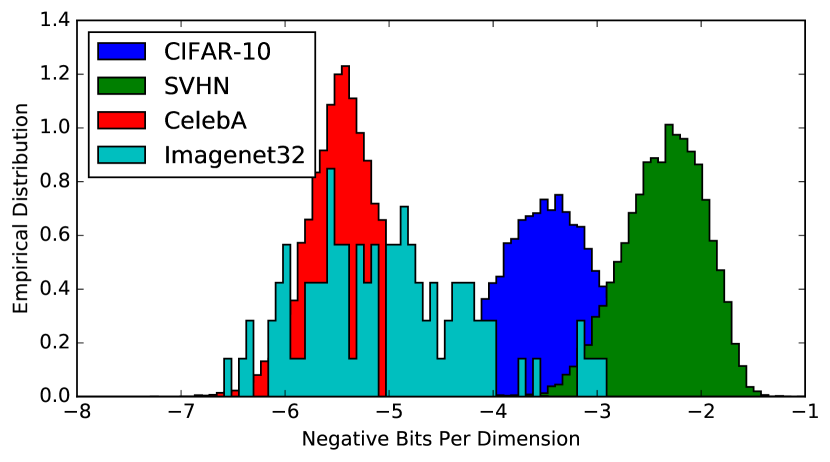
An earlier version of this paper, concurrently with work by Nalisnick et al. (2018), and Hendrycks et al. (2018) showed that likelihood models can be fooled by OoD datasets that are not even adversarial by construction. As shown in Figure 1, a likelihood model trained on the CIFAR-10 dataset yields higher likelihood predictions on SVHN images than the CIFAR-10 training data itself! For a flow-based model with an isotropic Gaussian prior, this implies that SVHN images are systematically projected closer to the origin than the training data (Nalisnick et al., 2018).

Figure 1: Density estimation models are not robust to OoD inputs. A GLOW model (Kingma & Dhariwal, 2018) trained on CIFAR-10 assigns much higher likelihoods to samples from SVHN than samples from CIFAR-10. .

1.2 Likelihood and Typicality

Even if we could compute likelihoods exactly, it may not be a sufficient measure for scoring OoD inputs. It is tempting to suggest a simple one-tailed test in which lower likelihoods are OoD, but the intuition that in-distribution inputs should have the highest likelihoods does not hold in higher dimensions. For instance, consider an isotropic 784-dimensional Gaussian. A data point at the origin has maximum likelihood, and yet it is highly atypical because the vast majority of probability mass lies in an annulus of radius $\sqrt{784}$. Likelihoods can determine whether a point lies in the support of a distribution, but do not reveal where the probability mass is concentrated.

The main contributions of this work are as follows. First, we observe that likelihood models assign higher densities to OoD datasets than the ones they are trained on (SVHN for CIFAR-10 models, and MNIST for Fashion MNIST models). Second, we propose Generative Ensembles, an anomaly detection algorithm that combines density estimation with uncertainty estimation. Generative Ensembles are trained independently of the task model, and can be implemented using exact or approximate likelihood models. We also demonstrate how predictive uncertainty can be applied to robustify implicit GANs and leverage them for anomaly detection. Finally, we present yet another surprising property of deep generative models that warrants further explanation: density estimation should not be able to account for probability mass, and yet Generative Ensembles outperform OoD baselines on the majority of common OoD detection problems, and demonstrate competitive results with discriminative classification approaches on the Kaggle Credit Fraud dataset.

2 Related Work

Anomaly detection methods are closely intertwined with techniques used in uncertainty estimation, adversarial defense literature, and novelty detection.

2.1 Uncertainty Estimation

OoD detection is closely related to the problem of uncertainty estimation, whose goal is to yield calibrated confidence measures for a model’s predictive distribution $p({\textnormal{y}}|{\textnormal{x}})$. Well-calibrated uncertainty estimation integrates several forms of uncertainty into $p({\textnormal{y}}|{\textnormal{x}})$: model mispecification uncertainty (OoD detection of invalid inputs), aleatoric uncertainty (irreducible input noise for valid inputs), and epistemic uncertainty (unknown model parameters for valid inputs). In this paper, we study OoD detection in isolation; instead of considering whether $p({\textnormal{y}}|{\textnormal{x}})$ should be trusted for a given $x$, we are trying to determine whether $x$ should be fed into $p({\textnormal{y}}|{\textnormal{x}})$ at all.

Predictive uncertainty estimation is a model-dependent OoD technique because it depends on task-specific information (such as labels and task model architecture) in order to yield an integrated estimate of uncertainty. ODIN (Liang et al., 2018), MC Dropout (Gal & Ghahramani, 2016) and DeepEnsemble (Lakshminarayanan et al., 2017) model a calibrated predictive distribution for a classification task. Variational information bottleneck (VIB) (Alemi et al., 2018b) performs divergence estimation in latent space to detect OoD, but is technically a model-dependent technique because the latent code is trained jointly with the downstream classification task.

One limitation of model-dependent OoD techniques is that they may discard information about $p({\textnormal{x}})$ in learning the task-specific model $p(y|x)$. Consider a contrived binary classification model on images that learns to solve the task perfectly by discarding all information except the contents of the first pixel (no other information is preserved in the features). Subsequently, the model yields confident predictions on any distribution that happens to preserve identical first-pixel statistics. In contrast, density estimation in data space $x$ considers the structure of the entire input manifold, without bias towards a particular downstream task or task-specific compression.

In our work we estimate predictive uncertainty of the scoring model itself. Unlike predictive uncertainty methods applied to the task model’s predictions, Generative Ensembles do not require task-specific labels to train. Furthermore, model-independent OoD detection aids interpretation of predictive uncertainty by isolating the uncertainty component arising from OoD inputs.

2.2 Adversarial Defense

Although adversarial attack and defense literature usually considers small $L^{p}$-norm modifications to input (demonstrating the alarming sensitivity of neural networks), there is no such restriction in practice to the degree with which an input can be perturbed in a test setting. We consider adversarial inputs in the broader context of the OoD problem, where inputs can be swapped with other datasets, transformed and corrupted (Hendrycks & Dietterich, 2019), or are explicitly designed to fool the model.

Song et al. (2018) observe that adversarial examples designed to fool a downstream task tend to have low likelihoods under an independent generative model. They propose a “data purification” pipeline, where inputs are modified via gradient ascent on model likelihood before being passing to the classifier. Their evaluations are restricted to $L^{p}$-norm attacks on in-distribution inputs on the classifier, and do not take into account that the generative model itself may be susceptible to OoD errors. In fact, gradient ascent on model likelihood has the exact opposite of the desired effect when the input is OoD to begin with. In our experiments we measure the degree to which we can identify adversarially perturbed “rubbish inputs” as anomalies, and also note that adversarial examples for IWAE predictions have high rates under the latent code, making them suitable for anomaly detection.

2.3 Novelty Detection

When learning signals are scarce, such as in reinforcement learning (RL) with sparse rewards, the anomaly detection problem is re-framed as novelty detection, whereby an agent attempts to visit states that are OoD with respect to previous experience (Fu et al., 2017; Marsland, 2003). Anomaly detection algorithms, including our proposed Generative Ensembles, are directly applicable as novelty bonuses for exploration. However, we point out in Section 1.2 that likelihoods are deceiving in high dimensions - the point of highest density under a high-dimensional state distribution may be exceedingly rare.

3 Generative Ensembles

We introduce Generative Ensembles, a novel anomaly detection algorithm that combines likelihood models with predictive uncertainty estimation via ensemble variance. Concretely, an ensemble of generative models that compute exact or approximate likelihoods (autoregressive models, flow-based models, VAEs) are used to estimate the Watanabe-Akaike Information Criterion (WAIC).

3.1 Watanabe Akaike Information Criterion (WAIC)

First introduced in Watanabe (2010), the Watanabe-Akaike Information Criterion (WAIC) gives an asymptotically correct estimate of the gap between the training set and test set expectations. If we had access to samples from the true Bayesian posterior of a model, we could compute a corrected version of the expected log  (Watanabe, 2009):

$$\text{WAIC}(x)=\mathbb{E}_{\theta}[\log p_{\theta}({\textnormal{x}})]-\mathrm{Var}_{\theta}\left[\log p_{\theta}({\textnormal{x}})\right]$$ (1)

The correction term subtracts the variance in likelihoods across independent samples from the posterior. This acts to robustify our estimate, ensuring that points that are sensitive to the particular choice of posterior parameters are penalized.

In this work we do not have exact posterior samples, so we instead utilize independently trained model instances as a proxy for posterior samples, following (Lakshminarayanan et al., 2017). Being trained with Stochastic Gradient Descent (SGD), the independent models in the ensemble act as approximate posterior samples (Mandt et al., 2017).

3.2 Does WAIC Address Typicality?

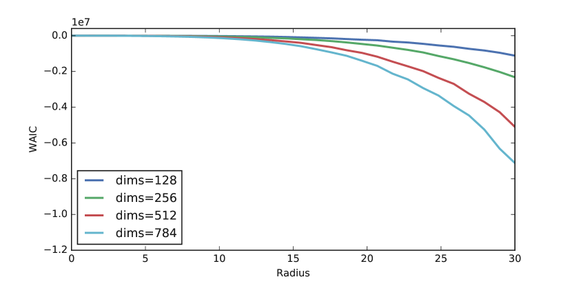
Although WAIC can protect models against likelihood estimation errors, we show via a toy model that it should not be able to distinguish whether a point is in the typical set. We illustrate this phenomena in Figure 2 on ensembles of Gaussians fitted to samples from an isotropic Gaussian with leave-one-out cross validation. Like likelihoods, the WAIC measure also decreases monotonically from the origin.

Figure 2: WAIC estimated using Jackknife resampling of data points drawn from an isotropic Gaussian, for an ensemble of size $N=10$. Lines correspond to a dimensionality of the data.

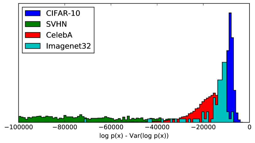
Given that SVHN latent codes lie interior to the CIFAR-10 annulus (Figure 1), WAIC should fail to distinguish SVHN as OoD. To our surprise, we show in Figure 3 and Table 1 that not only does WAIC reject SVHN as OoD, but it outperforms a baseline that does test for typicality by measuring the Euclidean distance to the origin!

Figure 3: We use ensembles of generative models to implement the Watanabe-Akaike Information Criterion (WAIC), which combines density estimation with uncertainty estimation. Histograms correspond to predictions over test sets from each dataset.

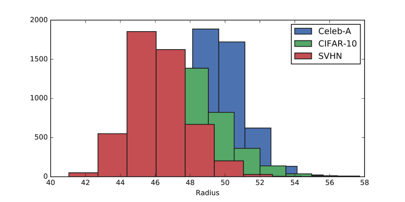
Glow models ought to map the training distribution (CIFAR-10) to a distribution whose probability mass is concentrated in an annulus of radius $\sqrt{3072}(\approx 55.4)$, but as we show in Figure 4, the Glow model actually maps CIFAR, SVHN, and Celeb-A to annuli whose mean radii span the range $42-54$. In our experiments, the variance of radii across models is larger for SVHN and Celeb-A than CIFAR-10, allowing the WAIC metric to correctly identify these as anomalies despite prior hypotheses that WAIC is insufficient.

Figure 4: Histogram of euclidean norms in latent space. Glow models map CIFAR-10, SVHN, and Celeb-A outside of the typical set.

3.3 Generative Ensembles of GANs

We describe how to improve GAN-based anomaly detection with ensembles. Although we cannot readily estimate WAIC with GANs, we can still leverage the principle of epistemic uncertainty to improve a GAN discriminator’s ability to detect OoD inputs.

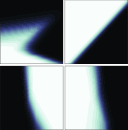
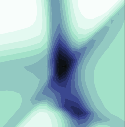
Figure 5b illustrates a simple 2D density modeling task where individual GAN discriminators – when trained to convergence – learn a discriminative boundary that does not adequately capture $p({\textnormal{x}})$. Unsurprisingly, a discriminative model tasked with classifying between $p({\textnormal{x}})$ and $q({\textnormal{x}})$ perform poorly when presented with inputs that belong to neither distribution. Despite this apparent shortcoming, GAN discriminators are still applied to successfully to anomaly detection problems (Schlegl et al., 2017; Deecke et al., 2018; Kliger & Fleishman, 2018).

Unlike discriminative anomaly classifiers, which model $p({\textnormal{x}})/q({\textnormal{x}})$ for a static $q({\textnormal{x}})$, the generative distribution $p_{\theta}({\textnormal{x}})$ of a GAN is trained jointly with the discriminator. The likelihood ratio $p({\textnormal{x}})/p_{\theta}({\textnormal{x}})$ learned by a GAN discriminator is uniquely randomized by GAN training dynamics on $\theta$ (Figure 5b). By training an ensemble of GANs, we can recover an (unnormalized) approximation of $p({\textnormal{x}})$ via decision boundaries between $p({\textnormal{x}})$ and randomly sampled $p_{\theta}({\textnormal{x}})$ (Figure 5c). We implement an anomaly detector using the variance of the discriminator logit, and show that although ensembling GANs lead to far more effective OoD detection than a single GAN (Supplemental Material), it does not outperform our WAIC-based Generative Ensembles.

Figure 5: In this toy example, we learn generative models for a 2D multivariate normal with identity covariance centered at (5, 5). (a) Explicit density models such as Normalizing Flows concentrate probability mass at the data distribution (b) Four independently trained GANs learn random discriminative boundaries, each corresponding to a different implied generator distribution. To ensure that the GAN discriminators form a clear discriminative boundary between $p({\textnormal{x}})$ and $p_{\theta}({\textnormal{x}})$, we train the discriminators an additional 10k steps to convergence. Each of these boundaries fails to enclose the true data distribution. (c) Predictive uncertainty over an ensemble of discriminators “fences in” the shared, low-variance region corresponding to $p({\textnormal{x}})$.

4 Experimental Results

Following the experiments proposed by (Liang et al., 2018) and (Alemi et al., 2018b), we train OoD models on MNIST, Fashion MNIST, CIFAR-10 datasets, and evaluate anomaly detection on test samples from other datasets. Source code for VAE and GAN experiments are located at https://github.com/hschoi1/rich_latent, and code for reproducing ODIN baselines are located at https://github.com/ericjang/odin.

We approximate likelihoods with two kinds of models, which we abbreviate as $p_{\theta}({\textnormal{x}})$ in Table 1. For MNIST and FashionMNIST, we estimate $\log p_{\theta}({\textnormal{x}})$ using a 16-sample Importance-Weighted AutoEncoder (IWAE) bound, and for CIFAR-10, we compute exact densities via Glow (Kingma & Dhariwal, 2018). We follow the protocol as suggested by (Lakshminarayanan et al., 2017) to use 5 models with different parameter initializations, and train them independently on the full training set with no bootstrapping. For VAE architectures we also evaluate the rate term $D_{\mathrm{KL}}(q_{\theta}(z|x)\|p(z))$, which corresponds to information loss between the latent inference distribution and prior (Alemi et al., 2018b). Glow uses a fixed isotropic Gaussian latent distribution, so we also devise a “typicality-aware baseline” that measures the euclidean distance $\left\|d\right\|$ to the closet point on a hypersphere of radius $\sqrt{3072}$. Finally, we report GAN-based anomaly detection in Appendix B. We extend the VAE example code from Tensorflow Probability (Dillon et al., 2017) to use a Masked Autoregressive Flow prior (Papamakarios et al., 2017), and train the model for 5k steps: The encoder consists of 5 convoluton layers. The decoder consists of 6 deconvolution layers followed by a convolution layer, and is trained using maximum likelihood under independent Bernoullis. We use a flexible learned prior $p_{\theta}({\textnormal{z}})$ in our VAE experiments, but did not observe a significant performance difference compared to the default mixture prior in the base VAE code sample. We use an alternating chain of 6 MAF bijectors and 6 random permutation bijectors. Models are trained with Adam ($\alpha=1\mathrm{e}{-3}$) with cosine decay on learning rate. Each Glow model uses the default implementation and training parameters from the Tensor2Tensor project (Vaswani et al., 2018) and is trained for 200k steps on a single GPU.

The baseline methods, ODIN and VIB, are dependent on a classification task and learn from the joint distribution of images and labels, while our methods use only images. For the VIB baseline, we use the rate term as the threshold variable. The experiments in (Alemi et al., 2018b) make use of (28, 28, 5) “location-aware” features concatenated to the model inputs, to assist in distinguishing spatial inhomogeneities in the data. In this work we train vanilla generative models with no special modifications, so we also train VIB without location-aware features. For CIFAR-10 experiments, we train VIB for 26 epochs and converge at 75.7% classification accuracy on the test set. All other experimental parameters for VIB are identical to those in (Alemi et al., 2018b).

Table 1: We train models on MNIST, Fashion MNIST, and CIFAR-10 and compare OoD classification ability to baseline methods using the threshold-independent Area Under ROC curve metric (AUROC). $p_{\theta}({\textnormal{x}})$ is a single-model likelihood approximation (IWAE for VAE, log-density for Glow). WAIC is the Watanabe-Akaike Information Criterion as estimated by the Generative Ensemble. ODIN results reproduced from (Liang et al., 2018). Best results for each task shown in bold.

OoD	ODIN	VIB	Rate	$p_{\theta}({\textnormal{x}})$	WAIC
MNIST	VAE
Omniglot	100	97.1	99.1	97.9	98.5
notMNIST	98.2	98.6	99.9	100	100
FashionMNIST	N/A	85.0	100	100	100
Uniform	100	76.6	100	100	100
Gaussian	100	99.2	100	100	100
HFlip	N/A	63.7	60.0	84.1	85.0
VFlip	N/A	75.1	61.8	80.0	81.3
Adv	N/A	N/A	100	0	100
FashionMNIST	VAE
Omniglot	N/A	94.3	83.2	56.8	79.6
notMNIST	N/A	89.6	92.8	92.0	98.7
MNIST	N/A	94.1	87.1	42.3	76.6
Uniform	N/A	79.6	99.0	100	100
Gaussian	N/A	89.3	100	100	100
HFlip	N/A	66.7	53.4	59.4	62.4
VFlip	N/A	90.2	58.6	66.8	74.0
Adv	N/A	N/A	100	0.1	100
OoD	ODIN	VIB	$\left\|d\right\|$	$p_{\theta}({\textnormal{x}})$	WAIC
CIFAR-10	Glow
CelebA	85.7	73.5	22.9	75.6	99.7
SVHN	89.9	52.8	74.4	7.5	100
ImageNet32	98.5	70.1	12.3	93.8	95.6
Uniform	99.9	54.0	100	100	100
Gaussian	100	45.8	100	100	100
HFlip	50.1	50.6	46.2	50.1	50.0
VFlip	84.2	51.2	44.0	50.6	50.4

Despite being trained without labels, our methods – in particular Generative Ensembles – outperform ODIN and VIB on most OoD tasks. The VAE rate term is robust to adversarial inputs on the IWAE, because the FGSM perturbation primarily minimizes the (larger) distortion component of the variational lower bound. The performance of VAE rate versus VIB also suggests that latent codes learned from generative objectives are more useful for OoD detection that latent codes learned via a classification-specific objective. Surprisingly, despite not being a general estimate of typicality, WAIC dramatically outperforms the $\left\|d\right\|$ baseline.

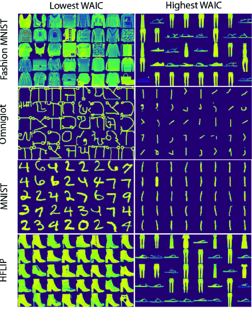
We present in Figure 6 images from OoD datasets with the smallest and largest WAICs, respectively. Models trained on FashionMNIST tend to assign higher likelihoods to straight, vertical objects like “1’s” and pants. It is not altogether surprising that AUROC scores on on the HFlip transformation was low, given that many pants, dresses are symmetric.

Figure 6: Left: lowest WAIC for each evaluation dataset. Right: highest WAIC for each evaluation dataset.

4.1 Credit Card Anomaly Detection

We consider the problem of detecting fraudulent credit card transactions from the Kaggle Credit Fraud Challenge (Dal Pozzolo et al., 2015). A conventional approach to fraud detection is to include a small fraction of fraudulent transactions in the training set, and then learn a discriminative classifier. Instead, we treat fraud detection as an anomaly detection problem where only normal credit card transactions are available at training time. This is motivated by realistic test scenarios, where an adversary is hardly restricted to generating data identically distributed to the training set.

We compare single likelihood models (16-sample IWAE) and Generative Ensembles (ensemble variance of IWAE) to a binary classifier baseline that has access to a training set of fraudulent transactions in Table 2. The classifier baseline is a fully-connected network with 2 hidden ReLU layers of 512 units, and is trained using a weighted sigmoid cross entropy loss (positive weight=580) with Dropout and RMSProp ($\alpha=1\mathrm{e}{-5}$). The VAE encoder and decoder are fully connected networks with single hidden layers (32 and 30 units, respectively) and trained using Adam ($\alpha=1\mathrm{e}{-3}$).

Unsurprisingly, the classifier baseline performs best because fraudulent test samples are distributed identically to fraudulent training samples. Even so, the single-model density estimation and Generative Ensemble achieve reasonable results.

4.2 Failure Analysis

In this section we discuss the experiments in which Generative Ensembles performed poorly, and suggest simple fixes to address these issues.

In our early experiments, we found that a VAE trained on Fashion MNIST performed poorly on all OoD datasets when using $p_{\theta}({\textnormal{x}})$ and WAIC metrics. This was surprising, since the same metrics performed well when the same VAE architecture was trained on MNIST. To explain this phenomenon, we show in Figure 7 inputs and VAE-decoded outputs from Fashion MNIST and MNIST test sets. Fashion MNIST images are reconstructed properly, while MNIST images are are barely recognizable after decoding.

Figure 7: Top: Inputs and decoded outputs from a VAE trained on Fashion MNIST($\beta=1$) for Fashion MNIST (left) and MNIST (right). Although Fashion MNIST inputs appear to be better reconstructed (suggesting higher likelihoods), they have comparable distortions to MNIST. The bottom row shows that Fashion MNIST and MNIST test samples have comparable rate-distortion scatter plots and IWAE histograms. This results in poor OoD detection of MNIST on Fashion MNIST images, which is mitigated by training with $\beta=.1$ to encourage better auto-encoding.

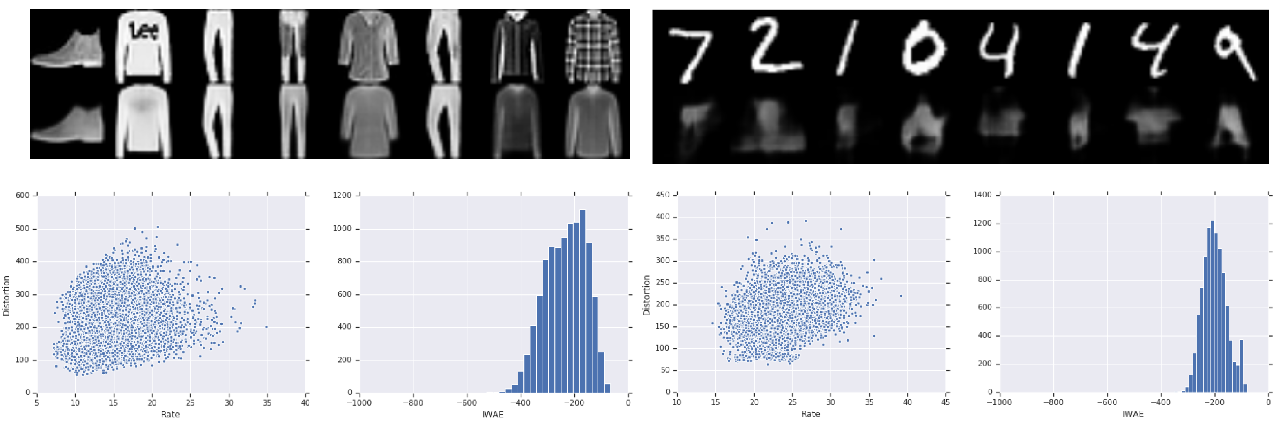
A VAE’s training objective can be interpreted as the sum of a pixel-wise autoencoding loss (distortion) and a “semantic” loss (rate). Even though Fashion MNIST appears to be better reconstructed in a semantic sense, the distortion values between the FashionMNIST and MNIST test datasets are numerically quite similar, as shown in Figure 7. Distortion terms make up the bulk of the IWAE predictions in our models, thus explaining why $p_{\theta}({\textnormal{x}})$ was not very discriminative when classifying OoD MNIST examples.

(Higgins et al., 2017) propose $\beta$-VAE, a simple modification to the standard VAE objective: $p(x|z)+\beta\cdot D_{\mathrm{KL}}(q_{\theta}(z|x)\|p(z))$. $\beta$ controls the relative balance between rate and distortion terms during training. Setting $\beta<1$ is a commonly prescribed fix for encouraging VAEs to approach the “autoencoding limit” and avoid posterior collapse (Alemi et al., 2018a). At test time, this results in higher-fidelity autoencoding at the expense of higher rates, which seems to be a more useful signal for identifying outliers than the total pixel distortion (also suggested by Table 1, column 4). Re-training the ensemble with $\beta=.1$ encourages a higher distortion penalty during training, and thereby fixes the OoD detection model.

Table 2: Comparison of density-based anomaly detection approaches to a classification baseline on the Kaggle Credit Card Fraud Dataset. The test set consists of 492 fraudulent transactions and 492 normal transactions. Threshold-independent metrics include False Positives at 95% True Positives (FPR@95%TPR), Area Under ROC (AUROC), and Average Precision (AP). Density-based models (Single IWAE, WAIC) are trained only on normal credit card transactions, while the classifier is trained on normal and fraudulent transactions. Arrows denote the direction of better scores.

Method	FPR@95%TPR $\downarrow$	AUROC $\uparrow$	AP $\uparrow$
Classifier	4.0	99.1	99.3
Single IWAE	15.7	94.6	92.0
WAIC	15.2	94.7	92.1

5 Discussion and Future Work

Out-of-Distribution (OoD) detection is a critical piece of infrastructure for ML applications where the test data distribution is not known at training time. Our paper has two main contributions. The more straightforward one is a novel technique for OoD detection in which ensembles of generative models can be used to estimate WAIC. We perform a comparison to prior techniques published in OoD literature to show that it is competitive with past models and argue for why OoD detection should be done “model-free”.

The other contribution is the intriguing observation that WAIC shouldn’t work! It has been established in the literature (Nalisnick et al., 2018; Hendrycks et al., 2018) that likelihood alone is not sufficient for determining whether data is out of distribution. Simply put, regions with high likelihood are not necessarily regions with high probability mass. It is premature, however, to invoke this explanation as the sole reason generative models trained on CIFAR-10 fail to identify SVHN as OoD, as we show, e pur si muove, that robust likelihood measures like WAIC can distinguish the samples correctly. As we show in Figure 4, the maximum likelihood objective typically used in flow-based models forces the training distribution (CIFAR-10) towards the region of maximum likelihood in latent space. We hypothesize that these datasets are quite different, different enough that the SVHN images likelihoods can be very sensitive to the initial conditions and architectural hyperparameters of the trained generative models. The surprising effectiveness of WAIC motivates further investigation into robust measures of typicality which incorporate both likelihood as well as some notion of local volume, as it is clear that there is an incomplete theoretical understanding within the research community of the limits of likelihood based OOD detection.

Furthermore, the observation that CIFAR-10 is mapped to an annulus of radius $<\sqrt{3072}$ is in itself quite disturbing, as it suggests that better flow-based generative models (for sampling) can be obtained by encouraging the training distribution to overlap better with the typical set in latent space.

Appendix A Terminology and Abbreviations

$p({\textnormal{x}})$	Training data distribution
$q({\textnormal{x}})$	OoD data distribution
$p_{\theta}({\textnormal{x}})$	Learned approximation of true distribution with parameters $\theta$. May be implicitly specified, i.e. a fully-observed density model
$q_{\theta}({\textnormal{x}})$	Learned approximation of OoD distribution with parameters $\theta$. May be implicitly specified, i.e. via a GAN discriminator that learns $p(x)/q_{\theta}({\textnormal{x}})$
OoD Input	Out-of-Distribution Input. Invalid input to a ML model
Anomaly	Synonym with OoD Input
Epistemic Uncertainty	Variance in a model’s predictive distribution arising from ignorance of true model parameters for a given input
Aleatoric Uncertainty	Variance in a model’s predictive distribution arising from inherent, irreducible noise in the inputs
Predictive Uncertainty	Variance of a model’s predictive distribution, which takes into account all of the above
MNIST	Dataset of handwritten digits (size: 28x28)
FashionMNIST	Dataset of clothing thumbnails (size: 28x28)
CIFAR-10	Dataset of color images (size: 32x32x3)
GAN	Generative Adversarial Network. See (Goodfellow et al., 2014)
FSGM	Fast Sign Gradient Method
WGAN	Wasserstein GAN. See (Arjovsky et al., 2017)
VAE	Variational Autoencoder. See (Kingma & Welling, 2014; Rezende et al., 2014)
Rate	$D_{\mathrm{KL}}(q_{\theta}(z|x)\|p(z))$ term in the VAE objective. Information loss between encoder distribution and prior over latent code
IWAE	Importance Weighted Autoencoder
GLOW	A generative model based on normalizing flows. See (Kingma & Dhariwal, 2018)
ODIN	Out-of-DIstribution detector for Neural networks. See (Liang et al., 2018)
VIB	Variational Information Bottleneck. See (Alemi et al., 2018b)
WAIC	Watanabe-Akaike Information Criterion. See (Watanabe, 2010)
AUROC	Area Under ROC Curve
FPR@95%TPR	False Positives at 95% True Positives
AP	Average Precision

Appendix B OoD Detection with GAN Discriminators

For MNIST, Fashion MNIST, and CIFAR-10 datasets, we train WGANs and fine tune the discriminators on stationary $p({\textnormal{x}})$ and $p_{\theta}({\textnormal{x}})$. Table 3 shows that ensemble variance of the discriminators, $\mathrm{Var}(D)$. Our WGAN model’s generator and discriminator share the same architecture with the VAE decoder and encoder, respectively. The discriminator has an additional linear projection layer to its prediction of the Wasserstein metric. We train all WGAN models for 20k generator updates. To ensure $D$ represents a meaningful discriminative boundary between the two distributions, we freeze the generator and fine-tune the discriminator for an additional 4k steps on stationary $p({\textnormal{x}})$ and $p_{\theta}({\textnormal{x}})$. For CIFAR-10 WGAN experiments, we change the first filter size in the discriminator from 7 to 8.

Table 3: We train models on MNIST, Fashion MNIST, and CIFAR-10 and compare OoD classification ability to one another using the threshold-independent Area Under ROC curve metric (AUROC). $D$ corresponds to single WGAN discriminators with 4k fine-tuning steps on stationary $p({\textnormal{x}})$, $q_{\theta}({\textnormal{x}})$. $\mathrm{Var}(D)$ is uncertainty estimated by an ensemble of discriminators. Rate is the $D_{\mathrm{KL}}$ term in the VAE objective. Best results for each task shown in bold.

OoD	D	Var(D)
MNIST
Omniglot	52.7	81.2
notMNIST	92.7	99.8
Fashion MNIST	81.5	100
Uniform	93.9	100
Gaussian	0.8	100
HFlip	44.5	60.0
VFlip	46.1	61.8
Adv	0.7	100
FashionMNIST
Omniglot	19.1	83.2
notMNIST	17.9	92.8
MNIST	45.1	87.1
Uniform	0	99.0
Gaussian	0	100
HFlip	54.7	53.4
VFlip	67.2	58.6
Adv	0	100
CIFAR-10
CelebA	57.2	74.4
SVHN	68.3	62.3
ImageNet32	49.1	62.6
Uniform	100	100
Gaussian	100	100
HFlip	51.6	51.3
VFlip	59.2	52.8

Appendix C VAE Architectural Details

We use a flexible learned prior $p_{\theta}({\textnormal{z}})$ in our VAE experiments, but did not observe a significant performance difference compared to the default mixture prior in the base VAE code sample. We use an alternating chain of 6 MAF bijectors and 6 random permutation bijectors. Each MAF bijector uses TensorFlow Probability’s default implementation with the following parameter:

⬇

shift_and_log_scale_fn=tfb.masked_autoregressive_default_template(

hidden_layers=(512, 512))

Models are trained with Adam ($\alpha=1\mathrm{e}{-3}$) with cosine decay on learning rate.

References

- Alemi et al. (2018a) Alemi, A., Poole, B., Fischer, I., Dillon, J., Saurous, R. A., and Murphy, K. Fixing a broken elbo. In International Conference on Machine Learning, pp. 159–168, 2018a.
- Alemi et al. (2018b) Alemi, A. A., Fischer, I., and Dillon, J. V. Uncertainty in the variational information bottleneck. arXiv preprint arXiv:1807.00906, 2018b.
- Arjovsky et al. (2017) Arjovsky, M., Chintala, S., and Bottou, L. Wasserstein gan. arXiv preprint arXiv:1701.07875, 2017.
- Bishop (1994) Bishop, C. M. Novelty detection and neural network validation. IEE Proceedings-Vision, Image and Signal processing, 141(4):217–222, 1994.
- Dal Pozzolo et al. (2015) Dal Pozzolo, A., Caelen, O., Johnson, R. A., and Bontempi, G. Calibrating probability with undersampling for unbalanced classification. In Computational Intelligence, 2015 IEEE Symposium Series on, pp. 159–166. IEEE, 2015.
- Deecke et al. (2018) Deecke, L., Vandermeulen, R., Ruff, L., Mandt, S., and Kloft, M. Anomaly detection with generative adversarial networks. 2018. URL https://openreview.net/forum?id=S1EfylZ0Z.
- Dillon et al. (2017) Dillon, J. V., Langmore, I., Tran, D., Brevdo, E., Vasudevan, S., Moore, D., Patton, B., Alemi, A., Hoffman, M., and Saurous, R. A. Tensorflow distributions. arXiv preprint arXiv:1711.10604, 2017.
- Dinh et al. (2014) Dinh, L., Krueger, D., and Bengio, Y. Nice: Non-linear independent components estimation. arXiv preprint arXiv:1410.8516, 2014.
- Fu et al. (2017) Fu, J., Co-Reyes, J., and Levine, S. Ex2: Exploration with exemplar models for deep reinforcement learning. In Advances in Neural Information Processing Systems, pp. 2577–2587, 2017.
- Gal & Ghahramani (2016) Gal, Y. and Ghahramani, Z. Dropout as a bayesian approximation: Representing model uncertainty in deep learning. In international conference on machine learning, pp. 1050–1059, 2016.
- Goodfellow et al. (2014) Goodfellow, I., Pouget-Abadie, J., Mirza, M., Xu, B., Warde-Farley, D., Ozair, S., Courville, A., and Bengio, Y. Generative adversarial nets. In Advances in neural information processing systems, pp. 2672–2680, 2014.
- Goodfellow et al. (2015) Goodfellow, I. J., Shlens, J., and Szegedy, C. Explaining and harnessing adversarial examples. International Conference on Learning Representations, 2015.
- Hendrycks & Dietterich (2019) Hendrycks, D. and Dietterich, T. Benchmarking neural network robustness to common corruptions and perturbations. In International Conference on Learning Representations, 2019.
- Hendrycks et al. (2018) Hendrycks, D., Mazeika, M., and Dietterich, T. G. Deep anomaly detection with outlier exposure. International Conference on Learning Representations, 2018.
- Higgins et al. (2017) Higgins, I., Matthey, L., Pal, A., Burgess, C., Glorot, X., Botvinick, M., Mohamed, S., and Lerchner, A. beta-vae: Learning basic visual concepts with a constrained variational framework. In International Conference on Learning Representations, 2017.
- Kingma & Dhariwal (2018) Kingma, D. P. and Dhariwal, P. Glow: Generative flow with invertible 1x1 convolutions. In Advances in Neural Information Processing Systems 31, pp. 10236–10245, 2018.
- Kingma & Welling (2014) Kingma, D. P. and Welling, M. Auto-encoding variational bayes. In International Conference on Learning Representations, 2014.
- Kliger & Fleishman (2018) Kliger, M. and Fleishman, S. Novelty detection with gan. arXiv preprint arXiv:1802.10560, 2018.
- Kos et al. (2018) Kos, J., Fischer, I., and Song, D. Adversarial examples for generative models. In 2018 IEEE Security and Privacy Workshops (SPW), pp. 36–42. IEEE, 2018.
- Lakshminarayanan et al. (2017) Lakshminarayanan, B., Pritzel, A., and Blundell, C. Simple and scalable predictive uncertainty estimation using deep ensembles. In Advances in Neural Information Processing Systems, pp. 6402–6413, 2017.
- Liang et al. (2018) Liang, S., Li, Y., and Srikant, R. Enhancing the reliability of out-of-distribution image detection in neural networks. In International Conference on Learning Representations, 2018.
- Mandt et al. (2017) Mandt, S., Hoffman, M. D., and Blei, D. M. Stochastic gradient descent as approximate bayesian inference. The Journal of Machine Learning Research, 18(1):4873–4907, 2017.
- Marsland (2003) Marsland, S. Novelty detection in learning systems. Neural computing surveys, 3(2):157–195, 2003.
- Nalisnick et al. (2018) Nalisnick, E., Matsukawa, A., Teh, Y. W., Gorur, D., and Lakshminarayanan, B. Do deep generative models know what they don’t know? In International Conference on Learning Representations, 2018.
- Nguyen et al. (2015) Nguyen, A., Yosinski, J., and Clune, J. Deep neural networks are easily fooled: High confidence predictions for unrecognizable images. In Proceedings of the IEEE Conference on Computer Vision and Pattern Recognition, pp. 427–436, 2015.
- Papamakarios et al. (2017) Papamakarios, G., Murray, I., and Pavlakou, T. Masked autoregressive flow for density estimation. In Advances in Neural Information Processing Systems, pp. 2338–2347, 2017.
- Rezende & Mohamed (2015) Rezende, D. J. and Mohamed, S. Variational inference with normalizing flows. In International Conference on Machine Learning, pp. 1530–1538, 2015.
- Rezende et al. (2014) Rezende, D. J., Mohamed, S., and Wierstra, D. Stochastic backpropagation and approximate inference in deep generative models. In International Conference on Machine Learning, 2014.
- Schlegl et al. (2017) Schlegl, T., Seeböck, P., Waldstein, S. M., Schmidt-Erfurth, U., and Langs, G. Unsupervised anomaly detection with generative adversarial networks to guide marker discovery. In International Conference on Information Processing in Medical Imaging, pp. 146–157. Springer, 2017.
- Song et al. (2018) Song, Y., Kim, T., Nowozin, S., Ermon, S., and Kushman, N. Pixeldefend: Leveraging generative models to understand and defend against adversarial examples. In International Conference on Learning Representations, 2018.
- Szegedy et al. (2013) Szegedy, C., Zaremba, W., Sutskever, I., Bruna, J., Erhan, D., Goodfellow, I., and Fergus, R. Intriguing properties of neural networks. arXiv preprint arXiv:1312.6199, 2013.
- Uria et al. (2016) Uria, B., Côté, M.-A., Gregor, K., Murray, I., and Larochelle, H. Neural autoregressive distribution estimation. The Journal of Machine Learning Research, 17(1):7184–7220, 2016.
- Vaswani et al. (2017) Vaswani, A., Shazeer, N., Parmar, N., Uszkoreit, J., Jones, L., Gomez, A. N., Kaiser, Ł., and Polosukhin, I. Attention is all you need. In Advances in Neural Information Processing Systems, pp. 5998–6008, 2017.
- Vaswani et al. (2018) Vaswani, A., Bengio, S., Brevdo, E., Chollet, F., Gomez, A. N., Gouws, S., Jones, L., Kaiser, L., Kalchbrenner, N., Parmar, N., Sepassi, R., Shazeer, N., and Uszkoreit, J. Tensor2tensor for neural machine translation. CoRR, abs/1803.07416, 2018. URL http://arxiv.org/abs/1803.07416.
- Wang et al. (2018) Wang, T.-C., Liu, M.-Y., Zhu, J.-Y., Tao, A., Kautz, J., and Catanzaro, B. High-resolution image synthesis and semantic manipulation with conditional gans. In IEEE Conference on Computer Vision and Pattern Recognition (CVPR), volume 1, pp. 5, 2018.
- Watanabe (2009) Watanabe, S. Algebraic geometry and statistical learning theory, volume 25. Cambridge University Press, 2009.
- Watanabe (2010) Watanabe, S. Asymptotic equivalence of bayes cross validation and widely applicable information criterion in singular learning theory. Journal of Machine Learning Research, 11(Dec):3571–3594, 2010.