Controlling synchronization in coupled area-preserving maps using stickiness

Abstract

Unidirectionally coupled area-preserving maps with a mixed phase space may show identical synchronization in the sticky neighborhood of the regular islands. We use this fact to devise numerical procedures to control (delay and expedite) the process of synchronization in two standard maps coupled under the Pecora-Carroll coupling scheme. The delay method is based on controlled kicking of trajectories away from synchronization traps for as long as necessary. The method to expedite the process is achieved by a parameter perturbation technique which rapidly drives the chaotic trajectories to synchronization traps in the sticky neighborhoods of regular islands. We also discuss the limitations of these methods.

I Introduction

A low-dimensional Hamiltonian system commonly exhibits a mixed phase space i.e. regular structures and chaotic regions may co-exist at a given degree of nonlinearity. This mixed nature has interesting consequences for the transport properties of such systems, for instance, the existence of anomalous kinetics, Lévy processes and Lévy flights Klafter1994 ; Zaburdaev2015 , power law contributions to recurrence and other statistics, and the existence of dynamical traps Zaslavsky2002a ; Zaslavsky2002b . An intriguing region of a mixed phase space is the interface between regular regions and chaotic sea Mackay1984 ; Easton1993 . The dynamics in these neighborhoods are complex but fairly well understood Meiss2015 for low dimensional systems. The complexity arises from the fact that a chaotic trajectory spends an arbitrary long but finite time at the boundaries of regular islands before exiting to the chaotic sea. The intermittent tendency of chaotic trajectories to stay close to the regular boundaries is called stickiness. A major consequence of the stickiness is the existence of power law in the Poincaré recurrence times indicating algebraic decay for long times rather than exponential decay expected for normal transport. Therefore, due to stickiness, even a small regular island can influence the global transport properties of the system and decay of correlations. The phenomenon has been of great interest and continues to be studied on theoretical level Altmann2006 ; Altmann2010 ; Livorati2012 ; Bunimovich2012 ; Kruger2015 ; Lange2016 . In addition, stickiness has found application in several problems such as particle advection in fluids Babiano1994 ; Tel2005 , transport in plasma fusion devices Szezech2012 ; Martins2014 , celestial mechanics Efthymiopoulos1999 ; Harsoula2010 ; Harsoula2016 .

A surprising feature of stickiness has emerged in our earlier work Mahata2016 , we have looked at the effects of the mixed phase space on the synchronization in a system of two standard maps coupled in unidirectional drive-response configuration. We have shown that synchronization of chaotic trajectories of the drive and response maps typically occurs in the neighborhood of regular inlands as a consequence of stickiness in the region. This is the first instance, as far as we are aware, where stickiness have been found to influence synchronization in coupled chaotic systems. It is important to point out that a possible role of stickiness in Hamiltonian systems for synchronization was already predicted by Zaslavsky Zaslavsky2002b in beginning of the last decade. For a chaotic orbit, synchronization typically happens via an intermittent behavior in the phase difference of the drive and response maps. The sticky neighborhoods of a regular islands temporarily traps chaotic orbits. In such trapping regions in the phase space, parts of a chaotic trajectory are almost regular in time and allow for synchronization to occur. Such traps are characterized using the properties of the finite-time Lyapunov exponent Szezech2005 . In the context of our work, we will refer to these traps as synchronization traps. We further note that the behavior of the synchronization traps can be analyzed in a more quantitative way by analyzing the location and stability properties of the periodic orbits at the locations where synchronization takes place.

Synchronization in coupled chaotic systems, coupled map lattices and networks have been studied in details (for reviews, see Pecora1998 ; Boccaletti2002 ; Pecora2015 ). Coupled Hamiltonian systems are also known to show synchronization such as Measure synchronization Hampton1999 ; Wang2003 ; Vincent2005 ; Gupta2017 and identical synchronization Mahata2016 ; Das2017 . However, the ability to control synchronization based on the dynamics of the process has not been given much attention, until recently Grabow2011 ; Wang2016 . In realistic systems, the speed of synchronization may be significant. For example, in neurosciences, the speed of the visual and olfactory processing are interesting problems Thorpe1996 ; Uchida2003 .

In this paper, we intend to develop a couple of mechanisms to control synchronization process i.e. to increase and to reduce synchronization times based on the location of synchronization traps in the sticky neighborhood of regular islands in the phase space of the area-preserving system of the standard map. Our delay method is based on the knowledge of the sticky neighborhoods of a mixed phase space. A simple kicking mechanism is used to keep the drive trajectory away until the control mechanism is active. The system synchronizes when the control is removed. On the other hand, the method to reduce synchronization times is based on parameter perturbation which is a well-known mechanism for chaos control Boccaletti2000 ; Ott2008 ; Bolotin2009 . Our method may be viewed as an adaptation of the Ott-Grebogi-Yorke (OGY) method Ott1990 suitable for our unidirectionally coupled system. The OGY method is applicable, in principle, to a chaotic system for which a mathematical description is unavailable. This procedure seeks to stabilize a desired low-order unstable periodic orbits embedded in a chaotic attractor via time-dependent parameter perturbations. In another method proposed by Lai and Grebogi Lai1993a ; Lai1994 , two identical systems are synchronized through parameter perturbation. This method introduces coupling in the system only when parameter is perturbed. Another approach Nagai1996 uses an adaptive parameter perturbation at every iteration in order to synchronize two coupled system. However, our technique of perturbation is similar to the one proposed by Aston and Bird and by Lai et. al. Lai1993b . These methods are suitable extensions of the OGY method. In the former work, a parameter perturbation is used for a dissipative system to constrain chaotic trajectories in the vicinity to the synchronous manifold. The later work describes a chaos control method for a Hamiltonian system by stabilizing chaotic orbits around some desired unstable period orbit. The basic idea is to tune the parameter judiciously when a chaotic trajectory visits the neighborhood of a fixed or periodic point embedded in a chaotic attractor so as to restrict it in the vicinity. We also apply the perturbation locally to one of the periodic points which eventually forces the drive trajectory to a synchronization trap.

We demonstrate the mechanism at a specific value of the nonlinearly parameter (see Sec. III) where only two small period 2 islands exist in the phase space.

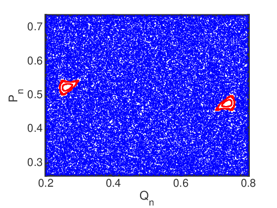
Figure 1: The phase space of the standard map at the parameter value K = 6.0. A couple of regular islands (shown in the color red) and a connected chaotic region (shown in the color blue).

The rest of the paper is organized in the following way: we explain the coupling scheme in Sec. II and the mechanism based on the location of synchronization traps is given in Sec. III. The numerical procedures to delay and advance synchronization times are demonstrated in Sec. IV and Sec. V respectively, and the paper ends with conclusions in Sec. VI including a discussion on limitations and implications.

II The Pecora Carroll’s unidirectional coupling scheme

The standard map is considered to be the prototypical example of a two-dimensional area-preserving map, and is given by:

$${}P_{n+1}=P_{n}+\frac{K}{2\pi}\sin(2\pi Q_{n})$$

$$Q_{n+1}=P_{n+1}+Q_{n}$$ (1)

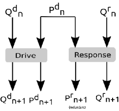
Figure 2: Schematic displaying the Pecora-Carroll method of coupling two standard map as explained in the text.

Here the subscript $n$ denotes the discrete time and $K$ is the nonlinearity parameter. These equations typically describe the evolution of two canonical variables $P$ and $Q$ which correspond to the momentum and co-ordinate in the Poincaré section of a freely moving rotator with interleaved periodic kicks. This system represents the behavior of a variety of systems such as charged particle confinement in mirror magnetic traps, particle dynamics in accelerator, comet dynamics in solar systems etc. Chirikov1960 ; Izraelev1980 ; Chirikov1989 ; Chirikov2008 Two-dimensional phase space plots of the standard map for the parameter value $K=6$ using a chaotic and a few regular initial conditions are shown in Fig. 1.

We now synchronize two standard maps, using the Pecora-Carroll scheme of synchronization using drive-response coupling Pecora1990 ; Pecora2015 . This system was first devised to synchronize the chaotic trajectories dissipative chaotic dynamical systems. Under this unidirectional coupling scheme, we duplicate the given map and couple the original and the duplicated map in a drive-response configuration. This means that the drive map evolves freely but the evolution of the response map is dependent on the drive. In this case, the $P$ value of the response system is set to the $P$ value of the drive system, at each iterate. A schematic is given to demonstrate the coupling scheme in Fig. 2.

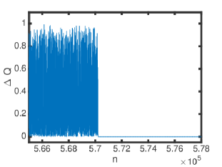
Figure 3: The variation of $\Delta Q=Q^{d}_{n}-Q^{r}_{n}$ of the coupled system at $K=6$ with iterations $n$. Synchronization is considered to be achieved when $\Delta Q<10^{-5}$ and remain so for the rest of the iterations. The iteration step $n$ at which synchronization occurs is called synchronization time $\tau$. For this case, $\tau=570246.$

The initial values of $Q$ in the drive and response maps are chosen arbitrarily, whereas the $P$ values are identical. The system is said to reach complete synchronization when both the $Q$ values of the drive and response systems evolve identically i.e.

$$\lim_{t\rightarrow\infty}(Q^{\textnormal{d}}_{n}-Q^{\textnormal{r}}_{n})=0.$$ (2)

Synchronization time is the least value of the iterate say, $\tau$, where $\Delta Q=Q^{d}-Q^{r}$ vanishes for all subsequent iterations:

$$(Q^{\textnormal{d}}_{n}-Q^{\textnormal{r}}_{n})=0;\hfill n\geq\bf{\tau}$$ (3)

In all of the computations reported in the work, two chaotic trajectories are considered to be synchronized to numerical accuracy, if the Euclidean distance between them is less than $10^{-5}$. An example is shown in Fig. 3. Here, we plot $\Delta Q=Q^{\textnormal{d}}_{n}-Q^{\textnormal{r}}_{n}$ for initial conditions $(P^{\textnormal{d}}_{0},Q^{\textnormal{d}}_{0},Q^{\textnormal{r}}_{0})=(0.569,0.906,0.106)$ at $K=6$. The synchronization time is found to be 5,70,246.

We now analyze synchronization of the coupled system using the master stability function Pecora1998 . Numerical procedures to control synchronization times will be discussed thereafter.

III Locating Synchronization Traps using Master stability function

A general drive-response system coupled unidirectionally may be described by the following set of equations:

$$\frac{d\mkern 1.5mu\overline{\mkern-1.5muX\mkern-1.5mu}\mkern 1.5mu_{\textnormal{d}}}{dt} =\mkern 1.5mu\overline{\mkern-1.5muF\mkern-1.5mu}\mkern 1.5mu(\mkern 1.5mu\overline{\mkern-1.5muX\mkern-1.5mu}\mkern 1.5mu_{\textnormal{d}})$$

$$\frac{d\mkern 1.5mu\overline{\mkern-1.5muX_{\textnormal{r}}\mkern-1.5mu}\mkern 1.5mu}{dt} =\mkern 1.5mu\overline{\mkern-1.5muF\mkern-1.5mu}\mkern 1.5mu(\mkern 1.5mu\overline{\mkern-1.5muX\mkern-1.5mu}\mkern 1.5mu_{\textnormal{r}})+\alpha E(\mkern 1.5mu\overline{\mkern-1.5muX\mkern-1.5mu}\mkern 1.5mu_{\textnormal{d}}-\mkern 1.5mu\overline{\mkern-1.5muX\mkern-1.5mu}\mkern 1.5mu_{\textnormal{r}}).$$ (4)

Here $\mkern 1.5mu\overline{\mkern-1.5muX\mkern-1.5mu}\mkern 1.5mu_{d}$ and $\mkern 1.5mu\overline{\mkern-1.5muX\mkern-1.5mu}\mkern 1.5mu_{r}$ are drive and response variables; the matrix $E$ determines the linear combination of the $\mkern 1.5mu\overline{\mkern-1.5muX\mkern-1.5mu}\mkern 1.5mu$ used in the difference and $\alpha$ is the coupling strength. For the map case, we have the following form

$$\mkern 1.5mu\overline{\mkern-1.5muX\mkern-1.5mu}\mkern 1.5mu^{\textnormal{d}}_{n+1} =\mkern 1.5mu\overline{\mkern-1.5muF\mkern-1.5mu}\mkern 1.5mu(\mkern 1.5mu\overline{\mkern-1.5muX\mkern-1.5mu}\mkern 1.5mu^{\textnormal{d}}_{n})$$

$$\mkern 1.5mu\overline{\mkern-1.5muX\mkern-1.5mu}\mkern 1.5mu^{\textnormal{r}}_{n+1} =\mkern 1.5mu\overline{\mkern-1.5muF\mkern-1.5mu}\mkern 1.5mu(\mkern 1.5mu\overline{\mkern-1.5muX\mkern-1.5mu}\mkern 1.5mu^{\textnormal{r}}_{n})+\alpha E(\mkern 1.5mu\overline{\mkern-1.5muX\mkern-1.5mu}\mkern 1.5mu^{\textnormal{d}}_{n}-\mkern 1.5mu\overline{\mkern-1.5muX\mkern-1.5mu}\mkern 1.5mu^{\textnormal{r}}_{n}).$$ (5)

Therefore, in the case of a general unidirectional coupling of two standard maps, we get

$$P^{\textnormal{d}}_{n+1} =P^{\textnormal{d}}_{n}+\frac{K}{2\pi}\sin(2\pi Q^{\textnormal{d}}_{n})$$

$$Q^{\textnormal{d}}_{n+1} =P^{\textnormal{d}}_{n+1}+Q^{\textnormal{d}}_{n}$$

$$P^{\textnormal{r}}_{n+1} =P^{\textnormal{r}}_{n}+\frac{K}{2\pi}\sin(2\pi Q^{\textnormal{r}}_{n})+\alpha(P^{\textnormal{d}}_{n}-P^{\textnormal{r}}_{n})$$

$$Q^{r}_{n+1} =P^{r}_{n+1}+Q^{r}_{n}.$$ (6)

We have chosen $E$ to be the matrix $\begin{bmatrix}1&0\\ 1&0\end{bmatrix}$.

To find the stability of the synchronous state, we first express Eq.(6) in terms of $P^{\perp}=P^{\textnormal{d}}-P^{\textnormal{r}}$ and $Q^{\perp}=Q^{\textnormal{d}}-Q^{\textnormal{r}}$, as follows

$$P^{\perp}_{n+1} =(1-\alpha)P^{\perp}_{n}+\frac{K}{2\pi}\sin(2\pi Q^{\textnormal{d}}_{n})-\frac{K}{2\pi}\sin(2\pi Q^{\textnormal{r}}_{n})$$

$$Q^{\perp}_{n+1} =(1-\alpha)P^{\perp}_{n}+Q^{\perp}_{n}+\frac{K}{2\pi}\sin(2\pi Q^{\textnormal{d}}_{n})$$ (7)

$$-\frac{K}{2\pi}\sin(2\pi Q^{\textnormal{r}}_{n}).$$

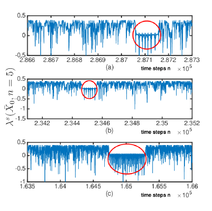
Figure 4: Fluctuations of time-5 FTLEs for three different set of initial conditions – $(P^{d}_{0},Q^{d}_{0},Q^{r}_{0})=(0.466,0.098,0.141)$ in (a), $(0.009,0.026,0.129)$ in (b), and $(0.553,0.554,0.396)$ in (c). The synchronization times in each cases are 287090, 234521, and 164782 respectively. The time scale on the $x$-axis indicates iteration steps $t$ at which time-5 FTLEs have been computed. The drop window in (a), (b), and (c) shown in ellipses in red occur around synchronization times. Synchronization of chaotic trajectories in the coupled system under study typically occurs in one of such traps.

We now write the variational equation for Eq.(III) by linearizing about $(P^{\textnormal{d}}_{n},Q^{\textnormal{d}}_{n})$

$$\left[\begin{array}[]{c}\delta P^{\perp}_{n+1}\\ \delta Q^{\perp}_{n+1}\end{array}\right]=\mathcal{M}(\alpha)\left[\begin{array}[]{c}\delta P^{\perp}_{n}\\ \delta Q^{\perp}_{n}\end{array}\right],$$ (8)

where the matrix $\mathcal{M}(\alpha)$ is given by

$$\mathcal{M}(\alpha)=\begin{bmatrix}1-\alpha&K\cos(2\pi Q^{\textnormal{d}}_{n})\\ 1-\alpha&1+K\cos(2\pi Q^{d}_{n})\end{bmatrix}.$$ (9)

This is the master stability equation for the unidirectionally coupled standard map. The variational equation (8) is the master stability equation for the coupled system under investigation. The associated largest Lyapunov exponent (LE) computed from the master stability equation is the master stability function (MSF) of the system, given by:

$$\lambda=\lim_{n\rightarrow\infty}\lim_{\delta\mkern 1.5mu\overline{\mkern-1.5muX\mkern-1.5mu}\mkern 1.5mu_{0}\rightarrow 0}\frac{1}{n}\sum^{n-1}_{i=0}\ln|JM^{n}(\mkern 1.5mu\overline{\mkern-1.5muX\mkern-1.5mu}\mkern 1.5mu_{i})|.$$ (10)

Here $n$ is a positive integer and $JM^{n}(\mkern 1.5mu\overline{\mkern-1.5muX\mkern-1.5mu}\mkern 1.5mu_{i})$ denotes the Jacobian matrix of the $n$-times iterated map. A negative value of the MSF (the largest non-zero LE) will ensure that $(P^{\perp},Q^{\perp})$ tend to zero indicating that the difference between $P$ and $Q$ will die out and the system will synchronize. Now, for the Pecora-Carroll approach, we set $\alpha=1$. This substitution simplifies the matrix in Eq.(9) which now reads

$$\mathcal{M}(1)=\begin{bmatrix}0&K\cos(2\pi Q^{\textnormal{d}}_{n})\\ 0&1+K\cos(2\pi Q^{d}_{n})\end{bmatrix},$$ (11)

The MSF should then be computed from the eigenvalues of the matrix $\mathcal{M}(1)$. It is easy to see that, for $\alpha=1$, one of the eigenvalues of $\mathcal{M}(1)$ is zero. Therefore, we need to consider only the non-zero eigenvalue which is $1+K\cos(2\pi Q^{d}_{n})$. The corresponding LE is given by

$$\lambda=\lim_{n\rightarrow\infty}\frac{1}{n}\sum^{n-1}_{i=0}\ln|1+K\cos(2\pi Q^{\textnormal{d}}_{i})|.$$ (12)

In general, we define the $kth$ time-$n$ LE associated with an initial point $\mkern 1.5mu\overline{\mkern-1.5muX\mkern-1.5mu}\mkern 1.5mu_{0}=(P_{0},Q_{0})$ for a map $M(P,Q)$ as

$$\lambda_{k}(\mkern 1.5mu\overline{\mkern-1.5muX\mkern-1.5mu}\mkern 1.5mu_{0};n)=\frac{1}{n}\sum^{n-1}_{i=0}\ln|JM^{n}(\mkern 1.5mu\overline{\mkern-1.5muX\mkern-1.5mu}\mkern 1.5mu_{i})|.$$ (13)

Here $n$ is a positive integer and $JM^{n}(\mkern 1.5mu\overline{\mkern-1.5muX\mkern-1.5mu}\mkern 1.5mu_{i})$ denotes the Jacobian matrix of the $n$-times iterated map. We extend this notion to the master stability function defined in the Sec. III i.e. the non-zero LE defined in Eq.(12) which takes the following finite time version

$$\lambda_{1}^{s}(\mkern 1.5mu\overline{\mkern-1.5muX\mkern-1.5mu}\mkern 1.5mu_{0};n)=\frac{1}{n}\sum^{n-1}_{i=0}\ln|1+K\cos(2\pi Q_{i})|.$$ (14)

The subscript ($k=1$) has been dropped hereafter as we have only one exponent to compute.

We plot the variation in the time-5 finite time Lyapunov exponent (FTLE) defined above at $K=6$. At the point of synchronization, the FTLE values attain a set of smaller values consistently in a small window, indicating the existence of a synchronization trap. In Fig. 4 , the three plots show the fluctuations of FTLE near the point of synchronization for three different sets of initial conditions - $(P^{d}_{0},Q^{d}_{0},Q^{r}_{0})=(0.466,0.098,0.141)$ in (a), $(0.009,0.026,0.129)$ in (b), and $(0.553,0.554,0.396)$ in (c) with synchronization times 287090, 234521, and 164782 respectively. The values on the $x$-axis indicate time steps at which averages are computed so that synchronization times and the temporal neighborhood are effectively captured in the plots wherein a temporary drop is clearly visible, indicated by ellipses in red. Synchronization of chaotic trajectories typically occurs in one of such traps. For details for the synchronization process, see  Mahata2016 ; Das2017 .

IV Delayed Synchronization Times

In order to develop a numerical technique to delay synchronization, we first have to identify the vicinity of regular islands in the phase space. A mechanism to suppress stickiness based on the knowledge of hyperbolic and non hyperbolic regions in the phase has been reported recently Kruger2015 . Our method, however, targets the trajectories themselves in the sticky region to delay the process. It is to be noted that the proposed procedure ignores the details of a rather complex hierarchy of structures around regular islands. We employ the edge-detection algorithm due to Benkadda et al. Benkadda1997 to identify the edges of regular islands in phase space. For the numerical procedure, we divide the phase space in $100\times 100$ grid. The edges of both islands are detected by applying the standard map to point initiated in the chaotic sea, for $10^{7}$ times. The edges thus detected is shown in Fig 5. We have chosen the proximity parameter $d=0.02$ i.e. Euclidean distance from points on the edge indicate the extent of the vicinity of the island. This vicinity, therefore, indicate the domain wherein the synchronization traps exist. To demonstrate this explicitly, we compare the phase angles, defined by $\theta=\tan^{-1}(\frac{Q}{P}$), of the points on numerically detected edges and the points of synchronization, as follows.

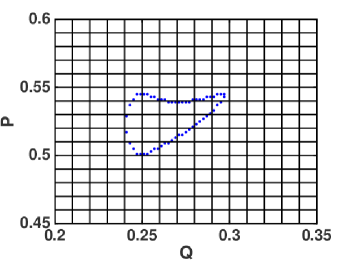
Figure 5: Example to detect the edge of a regular island in the phase space using edge detection algorithm due to Benkadda et al. Benkadda1997 .

In Fig. 6(a), we show the distribution of phase angles of the points on the edges of regular islands determined by the edge-detection algorithm. Bimodality of the distribution is due to the existence of two sharp islands in otherwise chaotic bulk in the phase space. We compare this with the phase angles corresponding to the points in the phase space at which synchronization of the chaotic trajectories occurs.

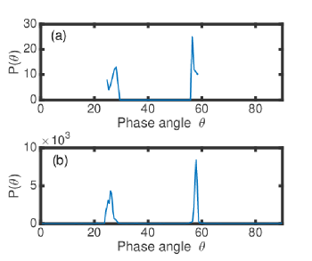
Figure 6: Numerical detection of synchronization traps (a) Distribution of phase angles of the points on the edges of regular islands determined by the edge detection algorithm. (b) Distribution of phase angles for points where synchronization occurs.

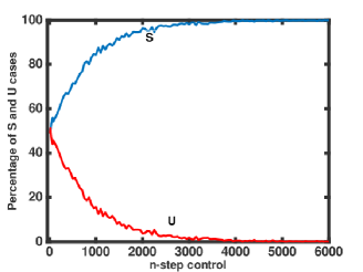
Figure 7: The curves indicate the percentages of (S) successful delays shown as the blue curve, and (U) undesirable fast synchronization shown as the red curve.

Fig. 6(b) shows the distribution of these phase angles for about 50 000 randomly chosen initial conditions for the drive and response maps that lead to synchronization. The locations of the peaks in the distribution shown in  6(a) approximately matches with this in  6(b). It is, therefore, visibly clear that synchronization occurs in the same angular domain of the phase space where the regular islands exist. Our numerically detected edges, thus correctly locate the synchronization traps in the phase space. We now discuss the control mechanism to delay synchronization time.

The proximity parameter $d_{0}=0.02$ defines the region in the neighborhood of the numerically detected edges wherein synchronization traps exist. The basic idea to control synchronization time is to identify the step at which the chaotic trajectory visits the numerically determined sticky neighborhood followed by a slight deflection so that the trajectory restarts at a point outside. Our procedure depends upon how many times we deflect the trajectory which will be referred to as step control. This means that if an $n-$step control is employed then, the trajectory will be kicked away from the domain $n$-times during its first $n$ visits i.e. once per visit. The deflection is achieved by adding a randomly generated fraction below $0.1$ to the point visiting the domain, and therefore the maximum deflection area is roughly $1\%$ of the phase space. This procedure applied on a given set of initial conditions of the drive and response maps, may result in four possibilities of synchronization time – (1) successful delay (S), (2) no delay (N), (3) failed to achieve synchronization (F), and (4) undesirable faster synchronization (U). Clearly, the only first possibility is the aim of the mechanism; the last one constitute a hazard while the other two are trivial.

For numerical implementation of the mechanism, we have considered $1000$ randomly chosen initial conditions from the chaotic sea of the phase space at $K=6$. The maps have been iterated for $10^{7}$ times in each case. The sticky domain is determined by the proximity parameter $d_{0}$ around the numerically detected edges of the regular islands. We demonstrate the effectiveness of the control procedure with respect to several $n-$step controls. The computations have been performed for $n\in\mathbb{A}$, where $\mathbb{A}=\{10,20,30,...,90,100,150,200,...,10000\}$.

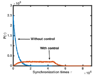
Figure 8: Distribution of synchronization times without n-step control (the blue curve) and with n-step control (the red curve). The control procedure delays synchronization times.

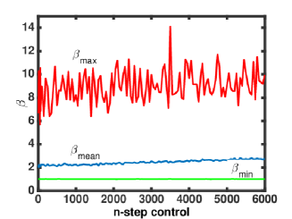
Figure 9: Variation of $\beta$ (maximum, minimum and average) which measures the strength of successful delays i.e. $\beta=\ln(\frac{\tau_{d}}{\tau_{0}}$). $\beta_{max}$ indicates the maximum delay time obtained at a give n-step control while $\beta_{mean}$ stands for the mean value around 2. This means that on an average, synchronization times re delayed by 100 times. The minimum value of $\beta$ remains 1 for the cases when no delay was obtained.

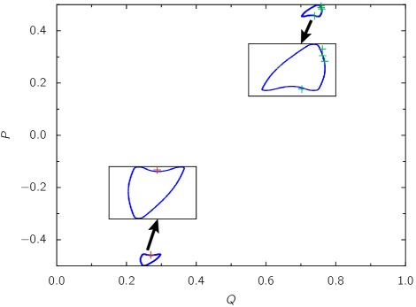
Figure 10: The phase space of a sample drive map at K = 6 (with $\epsilon=0.35$) displaying last 1500 iterates until synchronization takes place. The point of synchronization in the neighborhood of the lower island indicated by the sign ‘+’ in color red. The plot also shows, for illustration, other points of synchronization by the sign ‘+’ in color green for four other sample drive trajectories. The insets are magnified views of the two islands as indicated. Clearly, the parameter perturbation forces trajectories to the neighborhood of the regular islands where synchronization occurs.

Fig. 7 shows the percentage of successful delays (S) (on the y-axis) for a given $n-$step control (on the $x$-axis) up to $n=5500$ after which the successful cases are always $100\%$. We achieve about $50\%$ successful cases for $n=10$, which rises rapidly to $99\%$ for $n=2950$. It is to be noted that the average synchronization time without any control, $\tau_{avg}\sim 10^{5}$. Therefore, the n-steps required to obtain all successful delays is just about $3\%$ of $\tau_{avg}$. We also plot the distribution of synchronization times for successful cases and compare it against that of corresponding times without control in Fig 8. The long-tailed distribution of times without delay crosses over to a distribution which shows large flat region before a tail. The flat region indicate large number of successfully applied control with typical delay times of the order of $10^{6}$. For completeness, we show the decay in the number of undesired cases U in Fig 7. The cases F and N which are largely present for $n<10$, are extremely small in number and are neglected.

The degree of controlled synchronization $\beta$ may be defined as the ratio of synchronization times without numerical control, $\tau_{c}$ to synchronization times $\tau_{0}$ without control, i.e. $\beta=\ln(\frac{\tau_{d}}{\tau_{0}}$). Therefore, for successfully delayed synchronization $\beta>0$ indicating $\tau_{c}>\tau$. The plot in Fig. 9 shows the variation of $\beta$ i.e. $\beta_{min}$, $\beta_{mean}$, and $\beta_{max}$ indicating minimum, mean, and maximum $\beta$ for considered $n-$step controls. Clearly, we are able to attain $\beta_{max}$ values to be in the range $5$ to $14$ while mean values remain $\sim 2$. Therefore, we are successful in achieving significantly large delays in synchronization times.

There are a couple of limitations of the proposed control procedure. The deflection to the trajectory visiting the sticky domain should not insert it inside the regular island. The regular trajectories of the drive and response map are known to synchronize significantly faster and would result in the undesirable possibility (U). Therefore, an estimate of the size of regular islands, in addition to their locations must be known. These may be determined efficiently, as we have shown, using the edge-detection algorithm. The deflection area may then be chosen suitably. Another limitation is that the procedure is unable to impose a pre-determined delay to synchronization times. The random deflections simply keep the trajectories temporarily away from the synchronization traps in the sticky domain and synchronization may eventually occur after the removal of the control.

V Advanced Synchronization Times

We now explore the possibility to reduce synchronization times i.e. to expedite the process of synchronization. Once again, we will make use of the fact that synchronization traps typically exist in the sticky neighborhoods of the regular islands. The procedure is based on a parameter perturbation technique used to generate coherent structures in the phase space of area-preserving maps Gupte2007 . However, the technique may also be used to push chaotic trajectory to the neighborhood of periodic islands where synchronization traps exit. We describe the procedure briefly.

We take the standard map as in Eq. II with a modulo operation such that $-0.5\leq P_{n}\leq 0.5,0\leq Q_{n}\leq 1$. In this form, the standard map has a hyperbolic fixed point at $(P_{\textnormal{f}},Q_{\textnormal{f}})=(0,0)$,$(0,0.5)$. We perturb the parameter $K$ to $K-\epsilon$ if $|P-P_{\textnormal{f}}|<\delta$, $|Q-Q_{\textnormal{f}}|<\delta$. For $P$ and $Q$ outside this $\delta$-strip, $K$ does not change. It may be noted that the perturbed standard map remains to be area-preserving. The Jacobian $J$ is now given by:

$$J=\left(\begin{array}[]{cc}1+(K-\epsilon)\cos(2\pi Q_{n})&1\\ (K-\epsilon)\cos(2\pi Q_{n})&1\end{array}\right),$$

where, $\epsilon\neq 0$ if $|P_{f}-P_{n}|<\delta$, $|Q_{f}-Q_{n}|<\delta$
$\epsilon=0$, otherwise.

The determinant of this matrix $J$ remains 1. The phase space thus obtained for $K=6$ , $\delta=0.4$ and $\epsilon=0.35$ for the fixed point $(P_{\textnormal{f}},Q_{\textnormal{f}})=(0.0,0.0)$ is shown in Fig. 10. We have also performed computation for the other fixed point and with other modulo operations as well and results do not differ significantly. Our choice here of modulo operation and the fixed point $(P_{\textnormal{f}},Q_{\textnormal{f}})$ has some advantage over the others in terms of actual numerical values of synchronization times and the display of locations of the points where synchronization occurs.

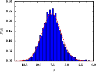
Figure 11: Distribution of degree of controlled synchronization, $P(\beta)$, mean is $-4.69$ and standard deviation $1.72$.

For the computations, we take 5 000 initial conditions chosen randomly from the chaotic region of the unperturbed standard map in the region $P_{0}\in\{-0.4,0.4\}$ and $Q_{0}\in\{0.3,0.7\}$. The total number of iterations used for each initial condition to check for synchronization is $10^{7}$ and threshold of synchronization is $10^{-5}$ as previously. The procedure has been applied to both drive and response map in accordance with our coupling scheme described above. We choose a patch around $(P_{\textnormal{f}},Q_{\textnormal{f}})$ of length $\delta=0.4$ which corresponds to about $16\%$ of the phase space area. We successfully obtain advance synchronization in more than $99\%$ of the cases among which a couple of instances has been shown in Fig. 10 – synchronization occurs in the neighborhood of one of the period 2 islands. The plots show the iterates of a sample drive trajectory until the point of synchronization (indicated by ‘+’ in green) is reached. Other ‘+’ signs in red indicate, for illustration, points of synchronization in four other cases in order to show that it occurs in the sticky neighborhoods.

We again define the degree of controlled synchronization as $\beta=\ln(\frac{\tau_{c}}{\tau}$). For advanced synchronization, $\beta<0$ indicating that synchronization times upon parameter perturbation is smaller than in the normal course (without any perturbation) i.e. $\tau_{c}<\tau$. The normalized probability distribution of $\beta$ in shown in Fig. 11, which may be fit with a Gaussian of the following form:

$$f(\beta)=\frac{1}{\sqrt{2\pi\sigma^{2}}}\exp\Big{(}-\frac{(\beta-\mu)^{2}}{2\sigma^{2}}\Big{)}.$$ (15)

We estimate the mean value $\mu\sim-4.69$ and standard deviation $\sigma\sim 1.72$ which corresponds to the fact that, on an average, advanced synchronization times thus obtained are about $10^{2}$ times smaller than the normal synchronization times with $95.5\%$ values are between $3$ to $3\times 10^{3}$ times smaller. Therefore, the synchronization times we obtained upon parameter perturbation is significantly smaller than the normal synchronization times. We would like to point that for a larger perturbation will be more efficient in reducing synchronization times. For example, at $\epsilon=2.0$ synchronization times are largely from $10$ to $10^{5}$ times smaller.

Thus, this parameter perturbation technique is an efficient way to reduce synchronization times with high efficiency. The value of the perturbation imposed should be chosen suitably as a very small may not have any influence on the synchronization process. The procedure also depends on the size and location of the patch wherein the control is applied.

VI Discussions and Conclusions

To summarize, we have developed numerical procedures to control synchronization in two identical standard maps coupled under the drive-response configuration. The procedure is based on the fact that synchronization in the system typically occurs in the sticky neighborhoods of the regular islands in the phase space. We have shown that a delay in synchronization can be obtained by kicking the trajectories slightly away from the domain temporarily. The efficiency of the procedure depends upon the number of steps employed in control. By applying the procedure to the system on merely $1\%$ of the phase space area (at $K=6$), we have successfully increased synchronization times. The maximum number of control steps that are used is $0.01\%$ of the total of number of iterations used throughout the computation. We showed that the procedure gives variety of delays. The limitations of this procedure are – (a) the deflection may insert the drive trajectory in the regular islands which would lead to undesirable faster synchronization, and (b) a predetermined synchronization time in not obtainable.

Furthermore, we have demonstrated a simple way to reduce synchronization times in the coupled system. Our technique targets the neighborhood of the periodic islands to obtain rapid synchronization. The distribution of degree of controlled synchronization times indicates the efficiency of the procedure – synchronization times are reduced upto a factor of $10^{3}$. We point out that the other techniques Ott1990 ; Lai1993b , in principle, could be applied to obtain synchronization if the trajectory are contained in synchronization traps long enough for synchronization to take place. In both the numerical procedures used in this work, we have ignored the complex hierarchical structures which is the origin of the sticky behavior of chaotic orbits in the phase space.

A possible future direction is to investigate the role of stickiness in phenomenon of measure synchronization (MS) in coupled Hamiltonian systems. We expect that location of sticky neighborhoods in the phase space may have an influence on the transitions involving different partial MS, complete MS, and desynchronization states Gupta2017 . Moreover, we note that the mechanism of parameter perturbation rapidly locates small regular islands in the mixed phase with a large chaotic component. Locations of these rather small periodic structures in a otherwise chaotic sea is thus determined quickly using only a small number of sample trajectories within a few hundred iterations (see Fig. 10). The classical problem of targeting invariant structures in Hamiltonian system Schroer1997 ; Cartwright2002 may be revisited if we understand the mechanism in detail and adapt it appropriately. As far as experimental situations are concerned, the stickiness is a known phenomenon with interesting consequences in a variety of systems such as intramolecular energy redistribution Sethi2012 , microwave ionization of Rydberg atoms Benenti2000 etc. In these contexts, a control method based on the location of the sticky neighborhoods could be useful.

- (1) J. Klafter and G. Zumofen, Lévy statistics in a Hamiltonian system, Phys. Rev. E 49, 4873 (1994).
- (2) V. Zaburdaev, S. Denisov, and J. Klafter, Lévy walks, Rev. Mod. Phys. 87, 483 (2015).
- (3) G. Zaslavsky, Chaos, fractional kinetics, and anomalous transport, Phy. Rep. 371, 461 (2002).
- (4) G. Zaslavsky, Dynamical traps, Physica D: Nonlinear Phenomena 168–169, 292 (2002).
- (5) R. MacKay, J. Meiss, and I. Percival, Transport in Hamiltonian systems, Physica D: Nonlinear Phenomena 13, 55 (1984).
- (6) R. W. Easton, J. D. Meiss, and S. Carver, Exit times and transport for symplectic twist maps, Chaos 3 (1993).
- (7) J. D. Meiss, Thirty years of turnstiles and transport, Chaos 25, 097602 (2015).
- (8) E. G. Altmann, A. E. Motter, and H. Kantz, Stickiness in Hamiltonian systems: From sharply divided to hierarchical phase space, Phys. Rev. E 73, 026207 (2006).
- (9) E. G. Altmann and A. Endler, Noise-enhanced trapping in chaotic scattering, Phys. Rev. Lett. 105, 244102 (2010).
- (10) A. L. P. Livorati, T. Kroetz, C. P. Dettmann, I. L. Caldas, and E. D. Leonel, Stickiness in a bouncer model: A slowing mechanism for Fermi acceleration, Phys. Rev. E 86, 036203 (2012).
- (11) L. A. Bunimovich and L. V. Vela-Arevalo, Many faces of stickiness in Hamiltonian systems, Chaos 22, 026103 (2012).
- (12) T. S. Krüger, P. P. Galuzio, T. d. L. Prado, R. L. Viana, J. D. Szezech, and S. R. Lopes, Mechanism for stickiness suppression during extreme events in Hamiltonian systems, Phys. Rev. E 91, 062903 (2015).
- (13) S. Lange, A. Bäcker, and R. Ketzmerick, What is the mechanism of power-law distributed Poincaré recurrences in higher-dimensional systems?, EPL 116, 30002 (2016).
- (14) A. Babiano, G. Boffetta, A. Provenzale, and A. Vulpiani, Chaotic advection in point vortex models and two‐dimensional turbulence, Phys. Fluids 6 (1994).
- (15) T. Tél, A. de Moura, C. Grebogi, and G. Károlyi, Chemical and biological activity in open flows: A dynamical system approach, Phys. Rep. 413, 91 (2005).
- (16) J. D. Szezech, I. L. Caldas, S. R. Lopes, P. J. Morrison, and R. L. Viana, Effective transport barriers in nontwist systems, Phys. Rev. E 86, 036206 (2012).
- (17) C. G. L. Martins, M. Roberto, and I. L. Caldas, Delineating the magnetic field line escape pattern and stickiness in a poloidally diverted tokamak, Phys. Plasmas 21, 082506 (2014).
- (18) C. Efthymiopoulos, G. Contopoulos, and N. Voglis, Cantori, islands and asymptotic curves in the stickiness region, Celest. Mech. Dyn. Astron. 73, 221 (1999).
- (19) M. Harsoula, C. Kalapotharakos, and G. Contopoulos, Asymptotic orbits in barred spiral galaxies, Mon. Notices Royal Astron. Soc. 411, 1111 (2011).
- (20) M. Harsoula, C. Efthymiopoulos, and G. Contopoulos, Analytical forms of chaotic spiral arms, Mon. Notices Royal Astron. Soc. 459, 3419 (2016).
- (21) S. Mahata, S. Das, and N. Gupte, Synchronization in area-preserving maps: Effects of mixed phase space and coherent structures, Phys. Rev. E 93, 062212 (2016).
- (22) J. Szezech Jr., S. Lopes, and R. Viana, Finite-time lyapunov spectrum for chaotic orbits of non-integrable Hamiltonian systems, Phy. Lett. A 335, 394 (2005).
- (23) L. M. Pecora and T. L. Carroll, Master stability functions for synchronized coupled systems, Phys. Rev. Lett. 80, 2109 (1998).
- (24) S. Boccaletti, J. Kurths, G. Osipov, D. Valladares, and C. Zhou, The synchronization of chaotic systems, Phys. Rep. 366, 1 (2002).
- (25) L. M. Pecora and T. L. Carroll, Synchronization of chaotic systems, Chaos 25, 097611 (2015).
- (26) A. Hampton and D. H. Zanette, Measure synchronization in Coupled Hamiltonian systems, Phys. Rev. Lett. 83, 2179 (1999).
- (27) X. Wang, Z. Ying, and G. Hu, Controlling Hamiltonian systems by using measure synchronization, Phys. Lett. A 298, 383 (2002).
- (28) U. E. Vincent, Measure synchronization in coupled Duffing Hamiltonian systems, New J. Phys. 7, 209 (2005).
- (29) S. Gupta, S. De, M. S. Janaki, and A. N. Sekar Iyengar, Exploring the route to measure synchronization in non-linearly coupled Hamiltonian systems, Chaos 27, 113103 (2017).
- (30) S. Das, S. Mahata, and N. Gupte, Synchronization, phase slips, and coherent structures in area-preserving maps, Proceedings of the Conference on Perspectives in Nonlinear Dynamics - 2016 1, 205 (2017).
- (31) C. Grabow, S. Grosskinsky, and M. Timme, Speed of complex network synchronization, Eur. Phys. J. B 84, 613 (2011).
- (32) S.-J. Wang, R.-H. Du, T. Jin, X.-S. Wu, and S.-X. Qu, Synchronous slowing down in coupled logistic maps via random network topology, Sci. Rep. 6, 1 (2016).
- (33) S. Thorpe, D. Fize, and C. Marlot, Speed of processing in the human visual system, Nature 381, 520 (1996).
- (34) N. Uchida and Z. F. Mainen, Speed and accuracy of olfactory discrimination in the rat, Nature Neuroscience 6, 1224 (2003).
- (35) S. Boccaletti, C. Grebogi, Y.-C. Lai, H. Mancini, and D. Maza, The control of chaos: theory and applications, Phys. Rep. 329, 103 (2000).
- (36) E. Ott, Controlling chaos, Scholarpedia 1, 1699 (2008).
- (37) Y. Bolotin, A. Tur, and V. Yanovsky, Chaos: Concepts, Control and Constructive Use, Understanding Complex Systems, Springer Berlin Heidelberg (2009).
- (38) E. Ott, C. Grebogi, and J. A. Yorke, Controlling chaos, Phys. Rev. Lett. 64, 1196 (1990).
- (39) Y.-C. Lai and C. Grebogi, Synchronization of chaotic trajectories using control, Phys. Rev. E 47, 2357 (1993).
- (40) Y.-C. Lai and C. Grebogi, Synchronization of spatiotemporal chaotic systems by feedback control, Phys. Rev. E 50, 1894 (1994).
- (41) Y. Nagai, X.-D. Hua, and Y.-C. Lai, Controlling on-off intermittent dynamics, Phys. Rev. E 54, 1190 (1996).
- (42) Y.-C. Lai, M. Ding, and C. Grebogi, Controlling Hamiltonian chaos, Phys. Rev. E 47, 86 (1993).
- (43) B. V. Chirikov, Resonance processes in magnetic traps, The Soviet Journal of Atomic Energy 6, 464 (1960).
- (44) F. Izraelev, Nearly linear mappings and their applications, Physica D: Nonlinear Phenomena 1, 243 (1980).
- (45) B. V. Chirikov and V. V. Vecheslavov, Chaotic dynamics of comet Halley, Astron. Astrophys. 221, 146 (1989).
- (46) B. Chirikov and D. Shepelyansky, Chirikov standard map, Scholarpedia 3, 3550 (2008).
- (47) L. M. Pecora and T. L. Carroll, Synchronization in chaotic systems, Phys. Rev. Lett. 64, 821 (1990).
- (48) S. Benkadda, S. Kassibrakis, R. B. White, and G. M. Zaslavsky, Self-similarity and transport in the standard map, Phys. Rev. E 55, 4909 (1997).
- (49) N. Gupte and A. Sharma, Creation of coherent structures in area-preserving maps, Phys. Lett. A 365, 295 (2007).
- (50) C. G. Schroer and E. Ott, Targeting in Hamiltonian systems that have mixed regular/chaotic phase spaces, Chaos: An Interdisciplinary Journal of Nonlinear Science 7, 512 (1997).
- (51) J. H. E. Cartwright, M. O. Magnasco, and O. Piro, Bailout embeddings, targeting of invariant tori, and the control of Hamiltonian chaos, Phys. Rev. E 65, 045203 (2002).
- (52) A. Sethi and S. Keshavamurthy, Driven coupled morse oscillators: visualizing the phase space and characterizing the transport, Mol. Phys. 110, 717 (2012).
- (53) G. Benenti, G. Casati, G. Maspero, and D. L. Shepelyansky, Quantum Poincaré Recurrences for a hydrogen atom in a microwave field, Phys. Rev. Lett. 84, 4088 (2000).