The Star Formation Reference Survey III: A Multi-wavelength View of Star Formation in Nearby Galaxies

Abstract

We present multi-wavelength global star formation rate (SFR) estimates for 326 galaxies from the Star Formation Reference Survey (SFRS) in order to determine the mutual scatter and range of validity of different indicators. The widely used empirical SFR recipes based on 1.4 GHz continuum, 8.0 $\mu$m polycyclic aromatic hydrocarbons (PAH), and a combination of far-infrared (FIR) plus ultraviolet (UV) emission are mutually consistent with scatter of $\la$0.3 dex. The scatter is even smaller, $\la$0.24 dex, in the intermediate luminosity range $9.3<\log(L_{60\,\micron}/{\mbox{L${}_{\odot}$}})<10.7$. The data prefer a non-linear relation between 1.4 GHz luminosity and other SFR measures. PAH luminosity underestimates SFR for galaxies with strong UV emission. A bolometric extinction correction to far-ultraviolet luminosity yields SFR within $0.2$ dex of the total SFR estimate, but extinction corrections based on UV spectral slope or nuclear Balmer decrement give SFRs that may differ from the total SFR by up to 2 dex. However, for the minority of galaxies with UV luminosity ${>}5\times 10^{9}$ L_⊙ or with implied far-UV extinction $<$1 mag, the UV spectral slope gives extinction corrections with 0.22 dex uncertainty.

1 Introduction

Star formation is critical for galaxy evolution. Stars have created almost all the elements heavier than helium in the Universe and play a key role in recycling dust and metals in galaxies. Hence the rate at which a galaxy forms stars is one of the most important drivers of its evolution. Understanding global trends in star formation rate (SFR henceforth) among different galaxy populations is required for interpreting the ‘Hubble sequence,’ which is a representation of not just the evolutionary trend in galaxy morphology but also gas content, mass, bars, dynamical structure, and environment, all of which influence the SFR (Kennicutt, 1998, and references therein). SFR measurements and the star formation rate density are therefore essential for constraining the models of structure formation in the Universe. However, until a few years ago, accurate measurements of SFR even in nearby galaxies were difficult owing to lack of knowledge of the effect of dust on different SFR tracers.

In addition to the standard optical spectral lines (e.g., H$\alpha$, [O ii]), the indicators most commonly used to quantify star formation in a galaxy are the global radio continuum, mid- and far-infrared (MIR and FIR), and ultraviolet (UV) emission. Different wavelengths trace stellar populations at different stages of evolution as well as different galaxy components. For instance, stars more massive than $\sim$8 M_⊙ produce the core-collapse supernovae whose remnants (SNRs) accelerate relativistic electrons, which have lifetimes $\la$100 Myr (Condon, 1992). The resulting non-thermal radio synchrotron emission, which dominates a galaxy’s radio luminosity at low frequencies ($\la$5 GHz), is therefore a measure of past formation of massive stars. Thermal radio emission, which dominates at high radio frequencies ($\ga$10 GHz; e.g., Klein & Emerson, 1981; Gioia et al., 1982; Tabatabaei et al., 2017) is a measure of current production of ionizing photons. The massive stars producing such photons have lifetimes of order 10 Myr, and high-frequency radio observations thus probe very recent SFR in star-forming and normal galaxies.

UV light is emitted predominantly by stars younger than around $200$ Myr and is therefore a good measure of SFR over time-scales of tens of Myr. But the interpretation of this indicator is hampered by the presence of dust clouds enshrouding young star-forming regions. Dust absorbs UV photons and reemits their energy at FIR wavelengths, making FIR luminosity a more reliable SFR indicator. For most star-forming galaxies, a combination of UV and FIR luminosity accounts for a major fraction of the galaxy’s bolometric luminosity.

Generally the FIR emission from any galaxy has at least two components, one originating from the interstellar dust heated by the diffuse radiation field and a second contribution from star formation activity in and near the H ii regions (Soifer et al., 1987, and references therein). If the second component can be measured, its FIR luminosity can be converted to an SFR measure.

Numerous attempts have been made to utilize the FIR–UV energy budget to quantify dust attenuation in various samples of galaxies selected at different wavelengths (e.g., Xu & Buat, 1995; Meurer et al., 1999; Buat et al., 2002, 2005; Cortese et al., 2006; da Cunha et al., 2010). One approach is to use the FIR/UV flux ratio (or the infrared excess IRX as it is more popularly known, e.g., Meurer et al., 1999; Kong et al., 2004; Seibert et al., 2005). An alternative is to use reddening inferred from the Balmer decrement (e.g., Buat et al., 2002; Gilbank et al., 2010) or from UV colour (e.g., Meurer et al., 1999; Lee et al., 2009; Gilbank et al., 2010). The reddening measure is then combined with an assumed extinction curve to yield extinction at UV wavelengths. The problem is understanding both random and systematic errors for the derived extinction values for different galaxy populations.

In order to understand the relation between indicators of star formation and dust extinction, the different SFR and extinction indicators need to be quantified and compared for a statistical sample of galaxies covering a wide range in physical and intrinsic properties and having known biases. This idea motivated the Star Formation Reference Survey (SFRS; Ashby et al., 2011, Paper I henceforth). Which SFR indicators can be used to estimate the global SFR of a galaxy? When are multi-wavelength data required? How closely does any single SFR indicator measure a galaxy’s ‘total’ SFR? Is the relation between individual SFR indicators universal for all types of star-forming galaxies? What are the advantages and disadvantages of different extinction indicators?

The primary purpose of this work is to present GALEX ultraviolet photometry for SFRS galaxies. By combining GALEX photometry with photometry at other wavelengths, we test and mutually calibrate widely used empirical formulas to calculate global SFRs for galaxies using tracers spanning all available wavelengths. In choosing among the many calibrations available in the literature, we have preferred those that give mutually consistent results. The wide ranges of morphologies, luminosities, sizes, SFRs, and stellar masses spanned by the SFRS galaxies, together with the sample’s well-defined selection criteria, makes it an ideal sample to quantify the relation between different SFR measures in nearby galaxies and hence a benchmark for comparing the SFR measures of high redshift galaxies. Studies such as this one have been performed elsewhere (e.g., Hopkins et al., 2001; Bell, 2003; Schmitt et al., 2006; Johnson et al., 2007; Zhu et al., 2008; Davies et al., 2016; Wang et al., 2016) but on samples often small or chosen without well-defined criteria or with narrow sample boundaries, where systematic deviations from the underlying correlations cannot be well explored. A recent study by Brown et al. (2017) used GALEX photometry as a SFR tracer, but their sample was restricted to galaxies with strong emission lines, and they did not use FIR at all.

This paper is organized as follows. §2 describes the datasets used in this paper, and §3 describes and compares the star formation tracers. §4 investigates extinction indicators and whether they can give useful measures of SFR. These are followed by a discussion of our findings in the context of the existing literature in §5, followed by a summary of our results in §6. Throughout this paper, star formation rates are based on a Salpeter IMF in the range 0.1–100 M_⊙.

2 The data

2.1 Sample selection

The SFRS (Paper I) is a statistically robust, representative sample of 367 star-forming galaxies in the local Universe. The sample selection criteria were defined objectively to guarantee that the SFRS has known biases and selection weights, making it possible to relate conclusions from the SFRS to magnitude-limited or volume-limited FIR-selected samples. Moreover, the SFRS spans the full ranges of properties exhibited by FIR-selected star-forming galaxies in the nearby Universe. While much larger galaxy samples exist, for huge samples it is difficult to obtain the complete data sets needed to explore multi-wavelength correlations. The SFRS is therefore an ideal tool for understanding the global properties of nearby ($z\la 0.1$) star-forming galaxies.

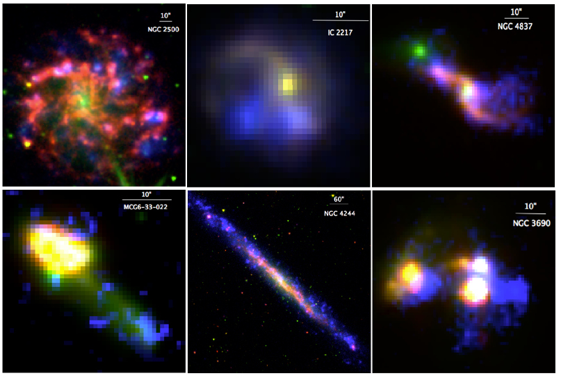
Figure 1: Six SFRS galaxies showing some of the variety in galaxy properties covered by this sample. colours represent IRAC 8.0 µm (red), 3.6 µm (green), and GALEX FUV (blue). Scale bars in each panel indicate angular sizes, which correspond to linear sizes of 0.72 kpc for NGC 2500, 3.7 kpc for IC 2217, 6.4 kpc for NGC 4837, 9.4 kpc for MCG 6-33-022, 1.25 kpc for NGC 4244, and 2.6 kpc for NGC 3690.

The SFRS was drawn from the PSC$z$ catalog (Saunders et al., 2000), an all-sky redshift survey of 15,000 galaxies observed by IRAS and brighter than 0.6 Jy at 60 µm. From this was drawn a representative subsample spanning the entire three-dimensional space formed by the 60 µm luminosity $L_{60}$, flux ratio $F_{60}/K_{s}$, and the IRAS flux density ratio $F_{100}/F_{60}$. $L_{60}$ is a proxy for the SFR, $F_{60}/K_{s}$ for specific star formation rate (sSFR), and $F_{100}/F_{60}$ measures FIR colour temperature ($T_{d}$) and thus heating intensity within star formation regions (Paper I). $T_{d}$ increases with increasing far infrared luminosity (Sanders & Mirabel, 1996), and thus $T_{d}$ may be related to the mode (‘normal’ or ‘starburst’ as described for example by Daddi et al. 2010, Rodighiero et al. 2011, or Elbaz et al. 2011) of star formation. Although the SFRS sample was drawn from FIR observations, it was constructed to include representative numbers of galaxies with $L_{60}\la 10^{6.5}$ L_⊙. Full details of the SFRS sample selection including distance estimates are given in Paper I. Figure 1 gives a glimpse of the wide range in galaxy sizes and morphologies covered by the SFRS. Metallicities (expressed as $\rm\log[O/H]+12$) range from 8.0 to 9.3 as measured by the ‘N2’ method (Maragkoudakis et al., 2018).

Because the SFRS sample was constructed to span the known ranges of galaxy SFR, sSFR, and $T_{d}$, uncommon types of galaxies (including, for example, edge-on galaxies) are over-represented in the sample. Galaxies with AGN are also included in the SFRS. In fact, the quasar 3C 273 and blazar OJ 287 were selected by the SFRS criteria, where each occupies its own unique cell in the selection matrix. Because these objects are dominated by luminous AGNs, they are not relevant to studies of local star formation and are excluded from this paper (decreasing the sample size to 367 galaxies). Other AGNs would not be as easily recognizable absent spectroscopic information. For example, SFRS 263 (=IRAS 13218+0552) is a Type-1 AGN (Maragkoudakis et al., 2018), and SFRS 270 (=IRAS 13349+2438) is a QSO (e.g., Lee et al., 2013). These are retained in our sample and will add to the observed scatter.

Paper I gives weights for SFRS galaxies which, if applied, make the sample proportional to the Saunders et al. (2000) PSC$z$ catalog. However, because the purpose of this paper is to test how well empirical SFR metrics work for all types of star-forming galaxies found in the local Universe, we have not applied these weights for the numerical calculations. This will make the derived scatter larger than would be the case for an unweighted sample, but the scatter will indicate the range that galaxies can occupy.

2.2 Ultraviolet data

The ultraviolet images for SFRS galaxies were retrieved from data releases 4/5 and 6 of the Galaxy Evolution EXplorer (GALEX; Martin et al., 2005; Morrissey et al., 2005). GALEX conducted an all-sky imaging survey along with targeted programs in two photometric bands: 1516 Å (‘far ultraviolet’ or FUV) and 2267 Å (‘near ultraviolet’ or NUV). The bulk of the SFRS sample consists of bright, nearby galaxies, and therefore no exposure time or brightness limit constraints were imposed while looking for a GALEX detection. Almost three quarters of the UV imaging data used in this paper were taken as part of the GALEX’s primary All-Sky Imaging Survey (AIS) with an effective exposure time of ${\sim}0.1$ ks. Most of the rest of the data come from the Nearby Galaxies Survey (NGS) with an effective exposure time of ${\sim}1.5$ ks. The remainder were observed as a part of other GALEX surveys as well as individual guest investigator programs. We imposed no constraint on the location of galaxy in the 1$\aas@@fstack{\circ}$2 GALEX field of view even though the point spread function varies across GALEX images, thus requiring non-negligible aperture corrections for faint sources detected away from the image centre. Whenever possible, we chose images where the target galaxy was closer to the centre of the field of view. Whenever a galaxy was observed as a part of more than one program, we chose the deepest observations. In total, GALEX imaging data were available for 326/367 (89 per cent) of the sample galaxies in at least one waveband. These 326 galaxies form the sample for this paper. The unobserved galaxies are mostly those near bright, blue stars that precluded GALEX imaging. Because this is a purely local effect, it should not bias our conclusions. Adopted distances and UV photometry for the sample galaxies are given in Table 1.

Table 1: GALEX data for SFRS galaxies (complete table available in appendix).

SFRS1	Name	$D$ (Mpc)1	FUV2	$\Delta$FUV	NUV2	$\Delta$NUV	$E(B-V)^{3}$
1	IC 486	114.4	18.179	0.029	17.575	0.014	0.040
2	IC 2217	76.1	16.434	0.013	15.939	0.006	0.041
3	NGC 2500	15.0	13.925	0.004	13.785	0.002	0.040
5	MCG 6-18-009	164.4	17.890	0.026	17.064	0.011	0.052
8	NGC 2532	77.6	15.417	0.008	14.862	0.004	0.054
9	UGC 4261	93.2	16.485	0.014	16.159	0.007	0.055
10	NGC 2535	61.6	15.708	0.010	15.290	0.004	0.043
11	NGC 2543	26.3	15.986	0.011	15.516	0.005	0.069
12	NGC 2537	15.0	14.964	0.007	14.752	0.003	0.054
13	IC 2233	13.7	15.000	0.007	14.805	0.004	0.052
14	IC 2239	88.5	19.177	0.046	18.041	0.016	0.053

Notes: 1. distances from Paper I based on $H_{0}=73$ km s^-1 Mpc^-1
2. AB magnitude
3. Milky Way colour excess in magnitudes from Schlegel, Finkbeiner, & Davis (1998).

2.3 Infrared, Radio, and Visible data

The Two Micron All Sky Survey (2MASS), Infrared Astronomical Satellite IRAS, and Spitzer/Infrared Array Camera (IRAC) imaging data are described in Paper I. In this paper we follow Helou et al. (1988) and calculate the FIR flux of galaxies as:

$$F_{\rm FIR}=1.26\times 10^{-14}(2.58f_{60}+f_{100})\quad\rm(Wm^{-2})$$ (1)

where $f_{60}$ and $f_{100}$ are the IRAS 60 and 100 µm flux densities in units of Jy. Equation 1 is based directly on observed flux densities with no extrapolation and represents flux emerging between 42 and 122 µm (Helou et al., 1988). The two shortest-wavelength WISE bands are close to Spitzer/IRAC bands, and WISE band 3 is close to IRAS 12 µm, so we expect our results to be directly applicable to SFR measurements from WISE. WISE band 4 is close to Spitzer/MIPS 24 µm, both interesting for SFR measurements but complicated by the presence of AGN. The SFRS will be useful for future investigation of this wavelength.

The 1.4 GHz radio data are all from Paper I. For most galaxies the data come from the NVSS (Condon et al., 1998) or from deeper observations taken with the same VLA configuration (D).

The visible spectroscopic data used in this paper were taken from the Data Release 13 (DR13) of the Sloan Digital Sky Survey (SDSS; Albareti et al., 2017) or from the central pixels of long-slit spectra (Maragkoudakis et al., 2018). The SDSS spectra were obtained using two fiber-fed double spectrographs covering a wavelength range of 3800–9200 Å with spectral resolving power varying between $1850<\lambda/\Delta\lambda<2200$. The 3″ fiber spectra are available for 189 SFRS galaxies, of which 187 have detectable H$\alpha$ line emission. The long-slit data refer to regions 3$\aas@@fstack{\prime\prime}$5 by 3″ in size and spectral resolving power $\sim$1000. Full details are given by Maragkoudakis et al. (2018).

2.4 Photometry and aperture corrections

The UV and NIR photometry were measured consistently using SExtractor (Bertin & Arnouts, 1996). The two GALEX images and the four IRAC mosaics were first registered using swarp (Bertin et al., 2002) to bring all six images to a common WCS and pixel size of 0$\aas@@fstack{\prime\prime}$867. SExtractor was then run in dual-image mode with objects detected on the 3.6 µm IRAC image (see §2.3). The 3.6 µm image was chosen for the initial reference because this band is most sensitive to galaxy starlight. All images were inspected to check whether tidal features visible in UV and/or IR were included in estimating the total magnitudes. If not, the relevant processes above were repeated with a more suitable detection image. For the excessively UV-bright (XUV) galaxies (Gil de Paz et al., 2007; Thilker et al., 2007) such as NGC 4395, the NUV image was used for aperture selection and for total flux estimates via SExtractor ‘MAG_AUTO’.

Next we applied the extended-source correction to the UV fluxes. Figure 4 of Morrissey et al. (2007) shows that the aperture correction for apertures of radius $<$3$\aas@@fstack{\prime\prime}$8 and $>$6″ are approximately linear. Hence, following Figure 4 of Morrissey et al. (2007) we binned our data into three sets with $r<3\aas@@fstack{\prime\prime}8$, $3\aas@@fstack{\prime\prime}8<r<6\arcsec$, and $r>6\arcsec$, where $r$ is the half-light radius from the 2MASS catalog (§2.3). To the first set we applied a linear correction of the form $Ar+B$, where $A=-0.5608(-0.6521)$ and $B=2.4912(3.0682)$ respectively in FUV(NUV). To the second set we applied the corrections suggested by Morrissey et al. (2007) for the 6″ radius aperture. To the third set we applied the linear correction by approximating the curve of growth from 6″ onwards such that $A=-0.0016(-0.0028)$ and $B=0.14(0.2128)$ respectively for FUV(NUV).

A recent catalog of GALEX measurements for 4138 nearby galaxies (Bai, Zou, Liu, & Wang, 2015) includes FUV measurements for 42 and NUV measurements for 73 SFRS galaxies. For the galaxies in common, the FUV magnitudes presented here are in the median 0.03 mag brighter than the Bai et al. D25 magnitudes and 0.07 mag fainter than their asymptotic magnitudes. Corresponding values for NUV are 0.02 mag brighter and 0.10 mag fainter respectively. The agreement in the medians shows that our calibration is on the same scale as that of Bai et al. Individual galaxies, however, show differences between our magnitudes and the Bai et al. D25 magnitudes with standard deviations of 0.29 and 0.23 mag in the FUV and NUV bands, respectively. These dispersions represent the effect of different choices of aperture and perhaps also subtraction of sky background and contaminating sources. We also compared the UV fluxes obtained for the SFRS galaxies with those of Dale et al. (2007) for six galaxies in common with the SINGS sample (Kennicutt et al., 2003) and found them to agree within the uncertainties.

2.5 Milky Way Extinction

Dust in the Milky Way attenuates light from external galaxies. The degree of extinction depends on position and may require a large correction in the UV wavebands. We applied a correction of $A_{\rm FUV}=8.29\times E(B-V)$ and $A_{\rm NUV}=8.18\times E(B-V)$ (Seibert et al., 2005), where the adopted colour excess values $E(B-V)$ come from the dust reddening maps of Schlegel, Finkbeiner, & Davis (1998). These reddening maps are based on the reprocessed composite of the COBE/DIRBE and IRAS/ISSA maps at 100 µm with the zodiacal foreground and confirmed point sources removed. For the SFRS galaxies, colour excesses are in the range $0.007\leq E(B-V)\leq 0.164$ with a median of $0.023$ mag and are listed in Table 1. For the subsample of SFRS galaxies analysed here, 95 per cent of the FUV corrections are less than 0.45 mag. Recent work (Lenz, Hensley, & Doré, 2017) confirms that the uncertainties in the corrections are generally negligible for current purposes.

3 Star Formation Rate indicators

3.1 Individual Star Formation Indicators

A measure of SFR wholly independent of emission at any other wavelength comes from the 1.4 GHz radio emission. This radio emission (Condon, 1992) comes mainly from non-thermal synchrotron radiation from the relativistic electrons in the remnants of core collapse supernovae. There is also a small contribution from thermal bremsstrahlung from H ii regions (Condon, 1992; Schmitt et al., 2006; Tabatabaei et al., 2017) and potentially from an active galactic nucleus. Unfortunately the theoretical ratio of radio emission to SFR depends on the uncertain mass cutoff for Type II supernovae (Sullivan et al., 2001). Therefore the calibration usually is taken from an empirical comparison in the local universe (e.g., Yun et al., 2001, Eq. 13) of the SFR density $\rho_{\rm SFR}$ to radio power density $U_{\rm SF}$ related to star formation (i.e., subtracting radio emission from active galactic nuclei):

$$({\rm SFR}_{\rm 1.4\,GHz}/{\mbox{M${}_{\odot}$}}\,{\rm yr^{-1}})=(5.9\pm 1.8)(L_{\rm 1.4\,GHz}/{10^{22}\rm\,W\,Hz^{-1}})\quad.$$ (2)

This relation was derived by combining an integrated 1.4 GHz luminosity density $U_{\rm SF}=2.4\times 10^{19}$ W Hz^-1 Mpc^-3 with $\rho_{\rm SFR}=0.014\pm 0.005$ M_⊙ yr^-1Mpc^-3 (both corrected to $H_{0}=73$ km s^-1 Mpc^-1). These values were derived for the IRAS 2 Jy sample of galaxies with $L_{\rm 1.4\,GHz}<10^{24}$ W Hz^-1. More recent values are $U_{\rm SF}=(2.17\pm 0.10)\times 10^{19}$ (Mauch & Sadler, 2007) and $\rho_{\rm SFR}=0.012\pm 0.001$ (González Delgado et al., 2016), which give almost the same ratio. Other estimates of the $\rho_{\rm SFR}$ differ by factors of 0.87–2.25 (Gilbank et al., 2010) depending on method. Tabatabaei et al. (2017) compared radio SFR to a range of other indicators and found calibrations of 0.94–2.0 times that of Equation 2. Purely theoretical calculations give SFRs 1.4 times (Schmitt et al., 2006) or 2 times (Tabatabaei et al., 2017) higher than Equation 2. The differences in calibration methods are the main uncertainty in Equation 2. We adopted the value shown because of its wide use and scaling consistent with other indicators.

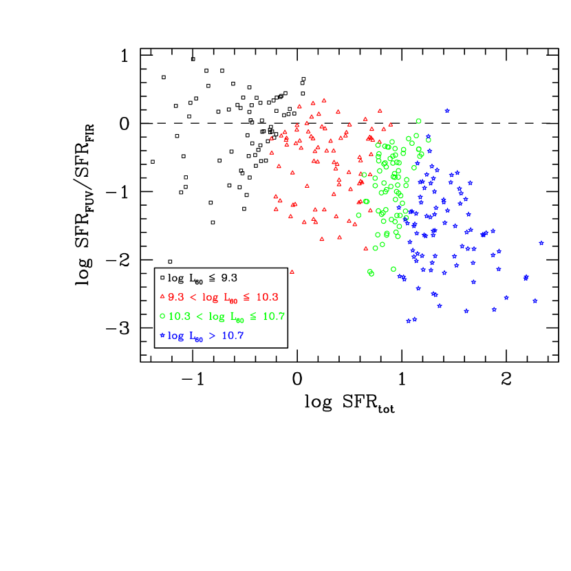
Figure 2: Ratio of SFRs calculated solely from FUV photometry to those derived solely from FIR photometry as a function of their sum. The symbols indicate individual galaxies coded by quartiles of $L_{60\,\micron}$: black squares for $L_{60\,\micron}<10^{9}$ L_⊙, red triangles for $10^{9}<L_{60\,\micron}<10^{10}$ L_⊙, green circles for $10^{10}<L_{60\,\micron}<10^{10.5}$ L_⊙, and blue stars for $L_{60\,\micron}>10^{10.5}$ L_⊙. The abscissa is SFR_tot from Equation 7, and the ordinate is the ratio of SFRs given by Equations 4 and 6.

A problem with the linear SFR${}_{\rm 1.4\,GHz}$ (Eq. 2) is that it tends to be too low at low SFR and too high at high SFR. Chi & Wolfendale (1990) and Bell (2003) among others have suggested that in low-luminosity (or low-SFR) galaxies, a fraction of the cosmic rays accelerated by SNRs may escape from the galaxy. This scenario might explain the underestimated SFR${}_{\rm 1.4\,GHz}$ of some low-luminosity galaxies in our sample. Tabatabaei et al. (2017) suggested that galaxies with high SFR might have stronger magnetic fields and a flatter energy distribution of relativistic electrons. This would imply stronger radio emission for a given SFR at high SFR. Davies et al. (2017) suggested a non-linear relation based on an essentially radio-selected sample of nearby galaxies:

$$({\rm SFR2}_{\rm 1.4\,GHz}/{\mbox{M${}_{\odot}$}}\,{\rm yr^{-1}})=5.25(L_{\rm 1.4\,GHz}/{10^{22}\,\rm W\,Hz^{-1}})^{0.75}\quad,$$ (3)

and Brown et al. (2017) found a nearly identical relation. A non-linear relation as in Equation 3 could compensate for cosmic ray escape at low SFR and increased radio emission at high SFR. Both the linear and non-linear relations are examined below.

An inevitable output of recent star formation is UV continuum emission from 1200–3200 Å. UV continuum can be therefore be used as an SFR indicator. We used the prescriptions provided by Iglesias-Páramo et al. (2006):

$$\log({\rm\mbox{SFR${}_{\rm FUV}$}/{\mbox{M${}_{\odot}$}}\,yr^{-1})}=\log(L_{\rm FUV}/{\mbox{L${}_{\odot}$}})-9.51\quad,$$ (4)

and

$$\log({\rm\mbox{SFR${}_{\rm NUV}$}/{\mbox{M${}_{\odot}$}}\,yr^{-1}})=\log(L_{\rm NUV}/{\mbox{L${}_{\odot}$}})-9.33\quad,$$ (5)

where $L_{\rm FUV}$ and $L_{\rm NUV}$ are the intrinsic FUV and NUV luminosities. Iglesias-Páramo et al. (2006) derived their calibrations from Starburst99 (Leitherer et al., 1999) assuming a solar metallicity. Hao et al. (2011) found SFR 20 per cent larger than given by Equation 4, and McQuinn, Skillman, Dolphin, & Mitchell (2015) suggested increasing the SFR_FUV calibration by a factor of 1.53. Neither will change our results because for the SFRS sample, the measured UV output represents only a small part of the total SFR measurement. The SFR could be overestimated if an old stellar population contributes significant UV emission. Indeed some elliptical galaxies, which have low SFR, show a ‘UV upturn’ (O’Connell, 1999). In most galaxies, this is due to residual star formation (Yi et al., 2011), but in a small fraction the UV emission can come from horizontal branch stars (e.g., Kjaergaard, 1987). While such emission will add slightly to the observed scatter in SFR relations, the small size of the effect even in elliptical galaxies shows that it will be negligible for most of the SFRS galaxies because the SFRS selection requires dust emission.

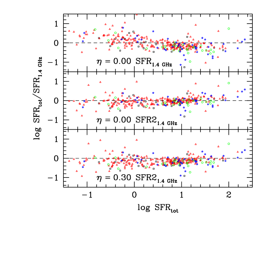
Figure 3: Ratio of SFR_tot (Eq. 7) to radio SFR as a function of SFR_tot. (top) Linear SFR${}_{\rm 1.4\,GHz}$ (Eq. 2) and $\eta=0$. (middle) Non-linear SFR2${}_{\rm 1.4\,GHz}$ (Eq. 3) and $\eta=0.0$. (bottom) Non-linear SFR2${}_{\rm 1.4\,GHz}$ and $\eta=0.3$. The abscissa for all panels uses $\eta=0$. Black squares, red triangles, green circles, and blue stars represent the four quartiles of 60 µm luminosity as indicated in the Figure 2 legend. Dashed lines show equality of the SFR measures being compared.

For all but the least dusty galaxies, most of the UV radiation emitted by young stars is absorbed by dust and reemitted in the FIR. Therefore, in order to use the measures in Equations 4 or 5, the observed UV emission has to be corrected for extinction by one of the methods discussed in Section 4. Alternatively, the reemitted FIR radiation itself can be used as the SFR tracer (Kennicutt, 1998). Here we adopt the estimate from Iglesias-Páramo et al. (2006):

$$\log{\rm(\mbox{SFR${}_{\rm FIR}$}}/{\rm{\mbox{M${}_{\odot}$}}\,yr^{-1}})=\log(L_{\rm FIR}/{\mbox{L${}_{\odot}$}})-9.75\quad,$$ (6)

where $L_{\rm FIR}$ is based on Equation 1 and the galaxy distance.

For the SFRS sample, the observed SFR_FUV is usually but not always negligible compared to SFR_FIR. This is evident from Figure 2, which also shows that the SFR_FUV/SFR_FIR ratio is a strong function of SFR_tot. Of our 326 galaxies with UV photometry, only 47 have $\mbox{SFR${}_{\rm FUV}$}>\mbox{SFR${}_{\rm FIR}$}$. This is not surprising because the SFRS sample is based on IRAS FIR detections. Despite that, UV-bright galaxies are represented in the SFRS sample because of its selection criteria.

$L_{\rm FIR}$ derived from Equation 1 differs from ‘Total Infrared Luminosity’ ($L_{\rm TIR}$), which takes into account all flux from 3 to 1100 µm. $L_{\rm TIR}$ has sometimes been used to derive SFR. $F_{\rm TIR}$ can be extrapolated from $F_{\rm FIR}$ and $f_{60}/f_{100}$ (Eq. 3 of Dale et al., 2001) or can be directly measured if Herschel/PACS data are available (Galametz et al., 2013). For galaxies in our sample, the IRAS extrapolation gives $1.38\leq F_{\rm TIR}/F_{\rm FIR}\leq 11$ with median 2.26 and standard deviation 0.26. Only 56 SFRS galaxies have any Herschel/PACS data available. For a few, the PACS 70 or 100 µm flux densities are more than a factor of 2 below the corresponding IRAS flux density. These galaxies are all notably extended in the IRAC images, and presumably the smaller Herschel beam is not picking up all the flux that IRAS saw. For the 38 SFRS galaxies having 160 µm PACS data and with PACS 70 or 100 µm data in agreement with IRAS, the median $F_{\rm TIR}$ is 0.10 dex higher than the IRAS extrapolation, and the dispersion of the ratio is 0.08 dex. This limited evidence suggests that extrapolating IRAS flux densities to derive $L_{\rm TIR}$ is reasonable, but $L_{\rm TIR}$ is not used here except where needed to compare with previous results.

The SFR_FIR measure suffers from two complications: some of the UV emission escapes from the galaxy without heating dust, and the FIR emission includes a contribution from dust heated by older stars (Sauvage & Thuan, 1992). Therefore an improved estimate is often assumed to be (Hirashita et al., 2003)

$$\rm\mbox{SFR${}_{\rm tot}$}=SFR_{\rm FUV}+(1-\eta)\mbox{SFR${}_{\rm FIR}$}$$ (7)

where SFR_FUV is calculated from the observed FUV emission, uncorrected for dust extinction, using Equation 4. The first term accounts for UV radiation that escapes without heating dust, and $\eta$ in the second term is the fraction of FIR luminosity produced by dust heated by old stellar populations. (Kennicutt & Evans 2012 and Calzetti 2013 have reviewed this subject.) Using $L_{\rm FIR}$ instead of $L_{\rm TIR}$ decreases the effect of dust heated by older stars because such dust is generally cooler than dust within star formation regions (Helou, 1986). Omitting the $\lambda>122$ µm radiation leads to smaller values of $\eta$.

The fraction $\eta$ of dust luminosity coming from old stars can be estimated using evolutionary synthesis models. Earlier studies involving starburst and luminous IR galaxies found $\eta\sim 0.6$ (e.g., Buat et al., 1999; Meurer et al., 1999; Gordon et al., 2000), but empirical values for normal star-forming galaxies are much lower (Bell, 2003; Hirashita et al., 2003; Buat et al., 2005; Kong et al., 2004; Hao et al., 2011), even though most studies have used TIR to derive $\eta$. For a diverse sample, Bell (2003) estimated the contribution of old stellar populations to IR luminosity to be 32$\pm$16 per cent for galaxies with $L_{\rm TIR}<10^{11}$L_⊙ and 9$\pm$5 per cent for LIRGs. Hirashita et al. (2003) found $\eta=0.40\pm 0.06$ for a sample of spiral and irregular galaxies in nearby galaxy clusters but $\eta=-0.04\pm 0.09$ (i.e., $\eta\approx 0$) for a sample of starburst galaxies selected at $\sim$1900 Å. For AKARI/FIS galaxies observed by SDSS/DR7 and GALEX, Buat et al. (2011) found $\eta=0.17\pm 0.10$. More recently, Boquien et al. (2016) studied galaxy regions $\sim$1 kpc in size and found $\eta=0.42$ for the luminosity-weighted average but ranging from $\sim$0.15 to $\sim$0.7 for different regions. Our results presented below are roughly equivalent to basing SFR on $L_{\rm TIR}$ and using $\eta=0.56$, the median value of $L_{\rm TIR}$/$L_{\rm FIR}$. However, using $L_{\rm TIR}$ would require either additional data beyond 100 µm or an uncertain extrapolation. As will be seen below, our choice to use $L_{\rm FIR}$ rather than $L_{\rm TIR}$ is justified by its success.

Table 2: SFR measures for SFRS galaxies (complete table available in appendix).

SFRS	SFRFUV	SFRNUV	SFR${}_{\rm 1.4\,GHz}$	SFR2${}_{\rm 1.4\,GHz}$	SFRFIR	SFRPAH	SFRtot
1	$-$0.18	0.06	0.97	0.81	0.57	0.74	0.64
2	0.16	0.36	0.89	0.76	0.65	0.84	0.78
3	$-$0.25	$-$0.19	$-$0.63	$-$0.25	$-$0.69	$-$0.53	$-$0.11
5	0.29	0.61	1.53	1.18	1.14	1.22	1.20
8	0.63	0.85	1.30	1.03	0.92	1.31	1.10
9	0.37	0.49	0.70	0.63	0.45	0.45	0.71
10	0.28	0.44	0.69	0.63	0.48	0.68	0.69
11	$-$0.49	$-$0.30	$-$0.22	0.02	$-$0.19	0.03	$-$0.01
12	$-$0.62	$-$0.54	$-$0.78	$-$0.34	$-$0.66	$-$0.77	$-$0.34
13	$-$0.72	$-$0.64	$-$1.58	$-$0.87	$-$1.30	$-$1.77	$-$0.61
14	$-$0.76	$-$0.31	0.84	0.73	0.85	0.66	0.86

Notes: 1. SFRs in units of $\rm\log(SFR/{\mbox{M${}_{\odot}$}}\,yr^{-1})$.
2. Paper I
3. $\log{\rm(\mbox{SFR${}_{\rm FIR}$}+\mbox{SFR${}_{\rm FUV}$})}$

Comparing the bottom two panels of Figure 3 shows that the main effect of varying $\eta$ is to change the scaling between SFR${}_{\rm 1.4\,GHz}$ (or SFR2${}_{\rm 1.4\,GHz}$) and SFR_tot and that the adopted calibration of Equation 3 gives a preference for $\eta\ll 0.3$. Adopting $\eta=0.3$ in place of $\eta=0$ would require decreasing the constant in Equation 3 by 0.12 dex. This is within the uncertainties of the calibration of SFR${}_{\rm 1.4\,GHz}$ (e.g., Yun et al., 2001; Hopkins et al., 2003; Schmitt et al., 2006; Gilbank et al., 2010; Davies et al., 2017). Using any SFR calibration to estimate $\eta$ is of limited use because the relative calibrations of different SFR indicators can always be adjusted (within limits) to make the sample median SFRs agree. As shown in the top two panels of Figure 3, the non-linear prescription for SFR${}_{\rm 1.4\,GHz}$ is strongly preferred because it removes the tendency for radio luminosity to underestimate SFR at low SFR values (Bell, 2003). Leaving aside the overall calibrations, in principle the scatter in the SFR_tot/SFR2${}_{\rm 1.4\,GHz}$  ratio can be used to estimate $\eta$. The dispersion of $\mbox{SFR2${}_{\rm 1.4\,GHz}$}/\mbox{SFR${}_{\rm tot}$}$ is smallest for $\eta=0$ (0.24 dex) but nearly constant with $\eta$ (0.25 dex for $\eta=0.3$). If we restrict the sample to the central two quartiles of 60 µm luminosity, the scatter is 0.16 dex for $\eta=0$ and 0.17 dex for $\eta=0.3$.

Table 3: Correlation ($y_{i}=a+bx_{i}$) comparing different log SFR distributions

SFR pairs ($x_{i}$–$y_{i}$)	Regression of $y_{i}$ on $x_{i}$						Regression of $x_{i}$ on $y_{i}$
	$-$$a_{1}$	$b_{1}$	$\sigma_{a}$	$\sigma_{b}$	$\sigma_{1}$		$-$$a_{2}$	$b_{2}$	$\sigma_{a}$	$\sigma_{b}$	$\sigma_{2}$
1.4 GHzNL–Total	$-$0.006	0.970	0.017	0.017	0.236		0.060	0.935	0.016	0.017	0.232
PAH–Total	0.148	0.830	0.018	0.018	0.284		$-$0.086	1.042	0.022	0.023	0.318
FIR–Total	0.198	0.863	0.008	0.008	0.127		$-$0.212	1.127	0.010	0.010	0.145
PAH–1.4 GHzNL	0.182	0.811	0.019	0.019	0.289		$-$0.118	1.055	0.023	0.024	0.330
PAH–FIR	$-$0.057	0.962	0.019	0.019	0.293		0.109	0.925	0.018	0.018	0.287
1.4 GHzNL–FIR	$-$0.233	1.118	0.017	0.018	0.243		0.237	0.827	0.013	0.013	0.209
1.4 GHz–Total	0.132	0.727	0.015	0.013	0.236		-0.109	1.247	0.021	0.022	0.309
PAH–1.4 GHz	0.054	1.081	0.025	0.025	0.386		0.031	0.791	0.021	0.018	0.330
1.4 GHz–FIR	-0.074	0.839	0.016	0.013	0.243		0.128	1.102	0.017	0.018	0.279
FUV–Total	0.848	0.673	0.041	0.053	0.633		$-$0.695	0.494	0.037	0.039	0.542
NUV–Total	0.711	0.841	0.033	0.052	0.576		$-$0.470	0.532	0.032	0.033	0.458
1.4 GHzNL–FUV	$-$0.691	0.467	0.039	0.041	0.560		0.848	0.614	0.042	0.054	0.642
1.4 GHz–FUV	$-$0.625	0.350	0.036	0.031	0.560		0.941	0.819	0.056	0.072	0.856
1.4 GHzNL–NUV	$-$0.470	0.510	0.034	0.035	0.478		0.724	0.778	0.034	0.053	0.591
1.4 GHz–NUV	$-$0.398	0.383	0.031	0.026	0.478		0.776	1.037	0.045	0.071	0.787
PAH–FUV	$-$0.631	0.429	0.035	0.035	0.549		0.811	0.733	0.047	0.060	0.718
PAH–NUV	$-$0.403	0.464	0.030	0.030	0.466		0.661	0.920	0.038	0.059	0.657
FUV–NUV	0.209	0.909	0.008	0.010	0.125		$-$0.237	1.055	0.008	0.012	0.135
FUV–FIR	0.701	0.653	0.050	0.065	0.771		$-$0.572	0.367	0.036	0.036	0.578
NUV–FIR	0.573	0.851	0.041	0.064	0.712		$-$0.345	0.413	0.031	0.031	0.496

¹Uncertainty in $a_{1}$ ($1\sigma$)
²Uncertainty in $b_{1}$ ($1\sigma$)
³Dispersion of sample from best fit relation (dex)
⁴Uncertainty in $a_{2}$ ($1\sigma$)
⁵Uncertainty in $b_{2}$ ($1\sigma$)
⁶Non-linear relation given by Eq. 3

The $\eta=0$ value implied by the scatter in SFR_tot/SFR2${}_{\rm 1.4\,GHz}$ differs from previous results. Our use of FIR rather than TIR is a principal but probably not the only reason for this: using the colour-dependent values of $\eta$ suggested by Boquien et al. (2016, their Fig. 6 and any of several colours from FUV to 3.6 µm) does not decrease the observed scatter. In fact, the calculated rms scatter in $\log{\rm(TIR/FIR)}$ for our sample is only 0.11 dex (Sec. 2.3). The real scatter is probably higher because the TIR/FIR ratio is based on an extrapolation using simple dust models (Dale et al., 2001), but the true TIR/FIR ratio cannot be evaluated without more observations at wavelengths longer than 100 µm. Better estimates of $\eta$ will require either much larger samples, better theoretical knowledge of the relative calibrations of SFR measures, or a new way of estimating values of $\eta$ for individual galaxies. In the following we use $\eta=0$ and non-linear SFR2${}_{\rm 1.4\,GHz}$ (Eq. 3) because these minimize both the observed scatter and the calibration offsets.

The last SFR measure we consider here is polycyclic aromatic hydrocarbon (PAH) molecular emission features. (See Calzetti 2011 for a review.) PAHs can form in galaxies from evolved stars, stellar mass loss, gas cloud collisions, or cooling flows and are excited by UV emission over a wide range of wavelengths. The PAH emission arises from photo-dissociation regions, which often surround (Helou et al., 2004) the H ii regions that mark the locations of massive stars. This makes PAH emission an indirect but still useful SFR tracer. The 8.0 µm IRAC band detects a complex of PAH features in low-redshift galaxies, and Wu et al. (2005) showed that the 8.0 µm dust luminosity correlates well with the 1.4 GHz and the 24 µm luminosity, both of which are star formation tracers. The 8.0 µm dust luminosity also correlates linearly with the MIPS 160 µm luminosity (Zhu et al., 2008) and non-linearly with the extinction-corrected Paschen-$\alpha$ luminosity (Calzetti et al., 2007). Calzetti et al. (2007), Zhu et al. (2008), Kennicutt et al. (2009), Shipley et al. (2016), and Maragkoudakis et al. (2017) among others have used PAH emission to estimate the SFR for galaxies, and Shipley et al. showed that of the various PAH features, the one at 7.7 µm correlates best with SFR as measured by their combination of 24 µm and H$\alpha$ emission.

For a majority of local galaxies seen by IRAC, the PAH emission dominates the 8.0 µm band (Pahre et al., 2004). However, a stellar continuum is still present especially in the early-type galaxies (Helou et al., 2004; Wu et al., 2005; Huang et al., 2007). To correct for this, we subtracted 0.227 times the 3.6 µm flux density from the observed 8.0 µm flux density to yield the 8.0 µm flux density attributable to dust (Huang et al., 2007). To convert the 8.0 µm dust luminosity to SFR, we have used the prescription of Wu et al. (2005) (also see Zhu et al., 2008):

$${\rm SFR_{\rm PAH}}/{\mbox{M${}_{\odot}$}}\,{\rm yr^{-1}}=\frac{\nu L_{\nu}{\rm[8.0\,\micron,dust]}}{1.57\times 10^{9}\,{\rm L_{\odot}}}\quad$$ (8)

with $L_{\nu}{\rm[8.0\,\micron,dust]}$ derived from the IRAC 8 µm flux density attributable to dust. Brown et al. (2017) found a non-linear relation between SFR and $L_{\rm PAH}$ (analogous to Equation 3 for 1.4 GHz). That would give a small overall decrease in dispersion (from 0.32 dex to 0.28 dex), improving the fit mainly for $\mbox{SFR${}_{\rm tot}$}\la 0.5$ M_⊙ yr^-1.

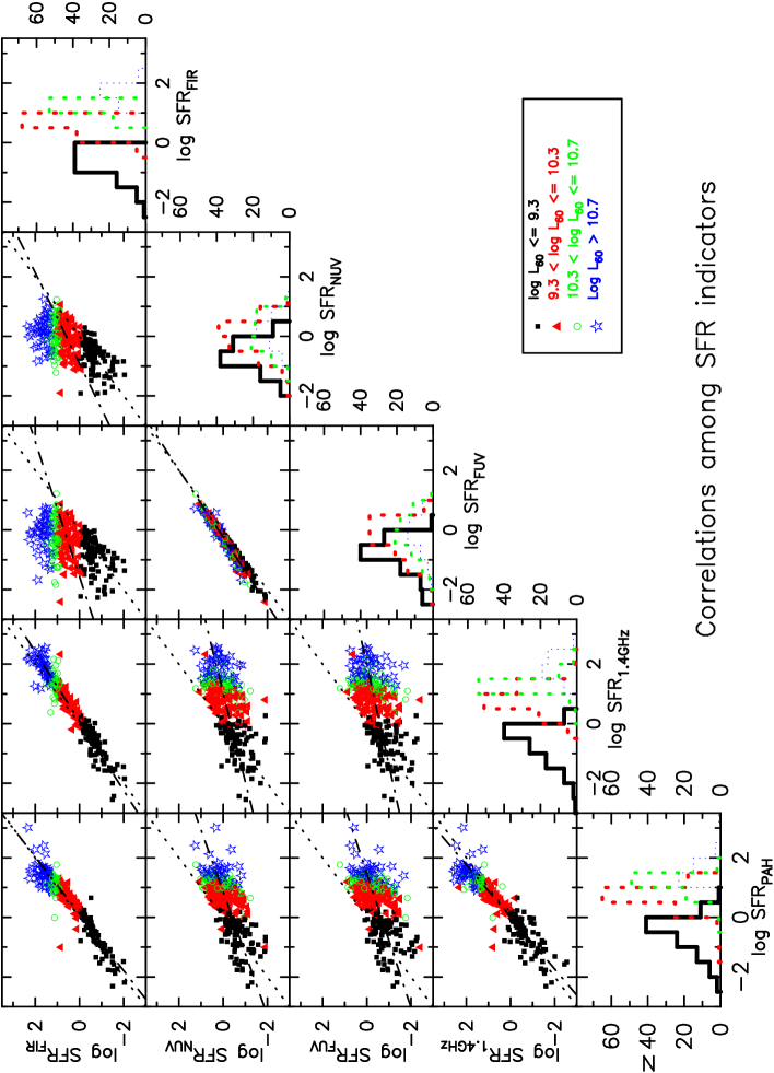
Figure 4: Comparison of SFR measures. Points represent SFRS galaxies with point types indicating quartiles of 60 µm luminosity as indicated in the legend. Dotted lines show equality of the respective SFR measures. Dot-dash lines show the best-fit relations. Histograms show the distribution of each SFR measure as indicated under the respective histogram with colours indicating the four quartiles of 60 µm luminosity.

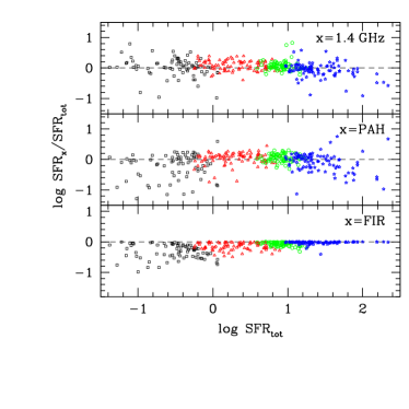
Figure 5: The ratio of SFR measured using (top to bottom) 1.4 GHz radio (non-linear measure as given by Eq. 3), PAH (Eq. 8), and FIR (Eq. 6) to the total SFR (Eq. 7) respectively. Symbols represent the four quartiles of 60 µm luminosity as indicated in the Figure 2 legend, and the dashed line corresponds to equality.

Table 4: Statistical properties of SFR distributions of SFRS galaxies using different SFR measures (all in $\log[{\rm SFR}/{\mbox{M${}_{\odot}$}}\,\rm yr^{-1}]$)

SFR	Mean	Std. deviation	Skewness	Median
FUV	$-$0.42	0.67	$-$0.57	$-$0.36
NUV	$-$0.17	0.62	$-$0.56	$-$0.12
U	0.19	0.97	$-$1.14	0.34
PAH	0.51	0.87	$-$0.75	0.77
FIR	0.43	0.88	$-$0.43	0.65
1.4 GHz	0.60	1.01	$-$0.54	0.88
1.4 GHzNL	0.59	0.76	$-$0.54	0.80
Total	0.57	0.77	$-$0.33	0.76

¹Linear relation given by Eq. 2
²Non-linear relation given by Eq. 3

Table 5: Results for statistical tests between different SFR distributions

SFR	$F$			Student’s $t$			K-S			Pearson’s $r$
Distributions	$F$	prob		$t$	prob		$D$	prob		$r$	prob
1.4 GHzNL–Total	1.337	0.009		$-$0.023	0.982		0.089	0.144		0.952	0.000
PAH–Total	1.261	0.037		$-$0.922	0.357		0.056	0.679		0.933	0.000
FIR–Total	1.307	0.016		$-$2.144	0.032		0.107	0.043		0.986	0.000
PAH–1.4 GHzNL	1.687	0.000		$-$0.956	0.339		0.100	0.074		0.927	0.000
PAH–FIR	1.036	0.751		1.164	0.245		0.079	0.247		0.945	0.000
1.4 GHzNL–FIR	1.748	0.000		2.250	0.025		0.156	0.001		0.961	0.000
1.4 GHz–Total	1.717	0.000		0.485	0.628		0.126	0.010		0.952	0.000
PAH–1.4 GHz	1.361	0.006		$-$1.266	0.206		0.127	0.009		0.927	0.000
1.4 GHz–FIR	1.314	0.014		2.332	0.020		0.156	0.001		0.961	0.000
FUV–Total	1.326	0.011		$-$17.460	0.000		0.540	0.000		0.565	0.000
NUV–Total	1.546	0.000		$-$13.400	0.000		0.479	0.000		0.657	0.000
1.4 GHzNL–FUV	1.008	0.939		18.844	0.000		0.546	0.000		0.526	0.000
1.4 GHz–FUV	2.276	0.000		15.220	0.000		0.546	0.000		0.526	0.000
1.4 GHz–NUV	2.654	0.000		11.706	0.000		0.506	0.000		0.621	0.000
1.4 GHzNL–NUV	1.156	0.191		14.536	0.000		0.506	0.000		0.621	0.000
PAH–FUV	1.673	0.000		15.280	0.000		0.553	0.000		0.573	0.000
PAH–NUV	1.951	0.000		11.420	0.000		0.485	0.000		0.667	0.000
FUV–NUV	1.166	0.167		$-$5.008	0.000		0.181	0.000		0.980	0.000
FUV–FIR	1.733	0.000		$-$13.840	0.000		0.503	0.000		0.478	0.000
NUV–FIR	2.021	0.000		$-$9.974	0.000		0.433	0.000		0.581	0.000

Notes–‘prob’ is the probability of the data under the null hypothesis.
¹The statistic $F\!=\!\sigma_{1}^{2}/\sigma_{2}^{2}$ where $\sigma_{i}^{2}$ is the variance.
²The statistic $t\!=\!(\overline{x_{1}}\!-\!\overline{x_{2}})/\sqrt{(\sigma_{1}^{2}/n_{1})\!+\!(\sigma_{2}^{2}/n_{2})}$ where $\overline{x_{i}}$ is the mean of a distribution of $n_{i}$ data points and variance $\sigma_{i}^{2}$.
³Non-linear relation given by Eq. 3
⁴Linear relation given by Eq. 2

All the SFR measures examined here are given in Table 1. For the majority of the sample, the statistical measurement uncertainty (i.e., from photon and detector noise) is below the systematic errors. For radio continuum imaging the calibration uncertainty is 3 per cent while the systematics add a further uncertainty of $0.45\sqrt{n}$ mJy to extended sources, where $n$ is the number of beams, each 45″ in diameter, covering the source. For the SFRS galaxies, $n\leq 5.7$ (Condon et al., 1991). The IRAS survey includes a uniform calibration for point sources of better than 10 per cent over nearly the entire sky (Soifer et al., 1987). For the IRAC and GALEX data, the calibration uncertainty is of the order of 3 per cent or better. Despite our efforts to choose apertures so as to give consistent total magnitudes, aperture uncertainties are probably at least 0.1 mag. As will be seen in Section 3.2, the uncertainties in the empirical relations used to convert luminosity to SFR are larger than these observational uncertainties.

3.2 Calibration of Individual SFR Tracers

The global radio and infrared SFR measures are in agreement with each other as shown in Figure 4. This is the case despite the prescriptions being based on very different underlying physics and their calibrations having been established from different samples. The uncorrected UV measures correlate with the others but are too low, especially at large SFR, as expected when extinction is ignored. The respective correlations, the standard deviation in fitted parameters, and the goodness of fit parameter $\chi^{2}$ are listed in Table 3. Table 4 lists some statistical properties of the different SFR distributions, and Table LABEL:tabstats gives results of statistical tests comparing them.

Figure 5 compares the indicators that are unaffected by extinction. The non-linear SFR2${}_{\rm 1.4\,GHz}$ shows an overall slope that would become steeper if the exponent in Equation 3 were made smaller (such as 0.66 in Eq. 2 of Bai, Zou, Liu, & Wang 2015). SFR_PAH is in good agreement with SFR_tot for most galaxies, but about 18 per cent of galaxies are outliers (8 with $\log(\mbox{SFR${}_{\rm PAH}$})-\log(\mbox{SFR${}_{\rm tot}$})>0.3$ and 51 with $\log(\mbox{SFR${}_{\rm PAH}$})-\log(\mbox{SFR${}_{\rm tot}$})<-0.3$). SFR_FIR is in good agreement with SFR_tot at high SFR, but it is up to $\sim$1 dex low at low SFR because this measure neglects UV light that escapes the galaxy without heating dust. This light is most important in low-SFR galaxies (Fig. 2).

Table 4 confirms that the SFR2${}_{\rm 1.4\,GHz}$, SFR_PAH, SFR_tot distributions are comparable in mean and median. This is also consistent with the $t$-test (Table LABEL:tabstats), which checks against the hypothesis that two distributions with different variances have the same mean. The K-S statistic (Table LABEL:tabstats) is consistent with all three being drawn from the same parent distribution. The mean and median for SFR_FIR are a little lower than the previous three because SFR_FIR neglects escaping UV light. Nevertheless, SFR_FIR is consistent with having been drawn from the same distribution of SFRs.

The ranges of SFR indicated by SFR_FIR, SFR_PAH, and SFR_tot are also similar as indicated by the respective sample standard deviations. The $F$-test measures the probability that two samples drawn from a single population would have variances differing by as much as the observed amount. The statistic $F$ (Table LABEL:tabstats) is the ratio of the two variances, and hence a value $\ll$1 or $\gg$1 indicates significantly different variances. Table LABEL:tabstats shows that the differences are at most marginally significant. In contrast, the linear SFR${}_{\rm 1.4\,GHz}$ shows a wider range than SFR_tot, consistent with its underestimating low SFR and overestimating high SFR. SFR2${}_{\rm 1.4\,GHz}$ compensates for that (and would overcompensate if the exponent in Equation 3 were made smaller).

As expected, the distributions of the UV SFRs differ from all others because the UV has not been corrected for extinction. Table 4 confirms that the mean of the UV SFRs is significantly below the monochromatic SFRs estimated at longer wavelengths.

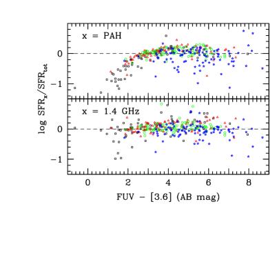
Figure 6: Ratio of inferred SFRs as a function of emerging UV radiation. The abscissa is the FUV to 3.6 µm colour as measured by IRAC in the same aperture used for the FUV magnitude. Upper panel shows SFR_PAH (Eq. 8, and lower panel shows non-linear SFR2${}_{\rm 1.4\,GHz}$ (Eq. 3). Point types show quartiles of 60 µm luminosity as indicated in the Figure 2 legend.

The good agreement between SFR_PAH and SFR_tot was also reported by Maragkoudakis et al. (2017). As noted above, most large deviations are in the sense that PAH underestimates the SFR, and most deviant galaxies are at the extreme ends of the luminosity distribution. The lack of PAH emission in low-luminosity galaxies has been documented previously (Boselli et al., 1998; Hogg et al., 2005) and attributed to lack of PAH grains (Wang & Heckman, 1996; Hopkins et al., 2001; Buat et al., 2005, among others). The low-luminosity galaxies can have deficient PAH emission if the galaxies are low in metallicity, i.e., lack the raw material to form PAHs, or if they are too young to have formed PAH yet. However, given that the shallow potential wells in these galaxies are unable to retain SNe ejecta for a prolonged duration, low metallicity might seem to be the most likely cause for the underestimated SFR_PAH for these galaxies (e.g., Leroy et al., 2006), and indeed Shipley et al. (2016) confirmed that galaxies with low metallicity have low PAH emission. However, Figure 6 shows that PAH deficiency is greatest in galaxies exhibiting strong UV radiation fields, suggesting that PAH destruction may be important. However, low metallicity could still be the underlying cause if the reason for the strong UV radiation field is low dust abundance. The high-luminosity galaxies may have a relatively intense radiation field that destroys the PAHs (e.g., Condon, 1992), but there is no evidence for that in the emerging UV radiation as seen in Figure 6. Because of dust extinction, however, the emerging UV radiation may not be characteristic of the local radiation fields where stars are forming.

The bottom panel of Figure 5 also shows the correlation between SFR_FIR and SFR_tot. As SFR_tot increases, the fraction of SFR traced by SFR_FIR increases markedly. For galaxies in the top luminosity quartile of the SFRS, virtually all the star formation is traced by FIR emission. For galaxies in the lowest luminosity quartile, SFR_FIR can underestimate SFR_tot by almost an order of magnitude for some galaxies, but for other galaxies with the same SFR, the SFR_FIR is the dominant contributor. Figure 2 is a more direct demonstration of the importance of escaping UV radiation as a function of luminosity or SFR.

4 Extinction Indicators

For a galaxy forming stars, the intrinsic UV luminosity is proportional to the SFR (Kennicutt 1998 and references therein). Dust, depending on its amount and distribution, absorbs some fraction of the UV and reradiates the energy in the FIR. If the extinction could be measured, the corrected UV flux would measure the total SFR.

In general, there are two types of extinction indicators for galaxies. One type is based on the ratio of FIR to UV luminosity ($\equiv$IRX). Such a ‘bolometric’ extinction indicator in effect gives a measure of total SFR as in Equation 7 but with a different formula to translate from observed flux densities to SFR. As for any method involving FIR emission, the measure is imperfect because older stars can also heat dust and also because our specific line of sight to a star forming region may not represent the average over all directions around that region because of both galaxy inclination and morphology of the dust distribution. The second type of method uses visible or UV spectral slope ($\beta$) (e.g., Meurer et al., 1999; Kong et al., 2004; Cortese et al., 2006; Gilbank et al., 2010; Overzier et al., 2011), Balmer decrement, or a similar measure of reddening, which is translated to extinction by means of a chosen reddening curve. Such ‘colour-excess’ (or ‘reddening’) methods are the only choice when FIR data are not available. A major problem is that colour excess depends critically on the dust geometry relative to the emitting stars (i.e., ‘foreground screen’ or ‘mixed slab’ approximations or ‘discrete clouds’ or a combination—see Charlot & Fall 2000 for discussion and modeling). Despite the complications, Meurer et al. (1999) (also see Cortese et al., 2006; Overzier et al., 2011) found an empirical relation between UV colour $\beta$ and IRX that gave rms scatter 0.3 dex in IRX in their UV-selected sample of local galaxies. The SFRS allows us to test how well such colour-excess methods work in a more representative sample.

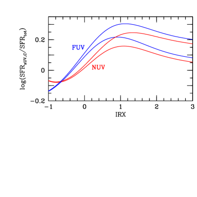
Figure 7: Ratio of SFR as calculated by empirical prescriptions (Buat et al., 2005) to SFR_tot. The abscissa IRX is the observed total infrared $F_{\rm TIR}$ to UV $\nu F_{\nu}$ flux ratio, making the ordinate depend on $F(60)/F(100)$. Blue curves show the ratio for FUV (Eq. 9) and the red curves for NUV (text footnote 12) for the 16th and 84th percentiles of $F(60)/F(100)$ of sample galaxies.

An empirical prescription (Buat et al., 2005) for the bolometric extinction $A_{\rm FUV}({\rm IRX})$ derived from IRX is

$$A_{\rm FUV}({\rm IRX})=-0.0333p^{3}+0.3522p^{2}+1.1960p+0.4967~{}~{},$$ (9)

where $p\equiv\log(L_{\rm TIR}/L_{\rm FUV})$. Figure 7 shows how this empirical prescription translates to SFR_tot for different values of IRX, and Figure 8 (upper panel) shows that SFR_FUV corrected for extinction by a bolometrically derived factor is close to $\rm SFR_{tot}$ for the SFRS sample, showing the ${\approx}0.2$ dex over-correction expected from Figure 7. The more luminous galaxies, those with $L_{60}>10^{10.5}$ L_⊙, tend to have larger IRX (as expected from Fig. 2) and therefore larger bolometric extinction. Figure 8 (lower panel) illustrates this relationship.

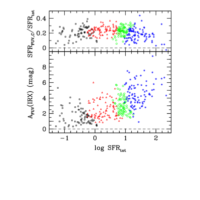
Figure 8: FUV extinction and resulting SFR as a function of SFR_tot. (Bottom:) FUV bolometric extinction $A_{\rm FUV}(IRX)$ (Eq. 9, original source Buat et al., 2005). Dashed line shows zero extinction. (Top:) Ratio of SFR computed from FUV corrected by bolometric extinction (Eq. 9) to SFR_tot. Dashed line shows equality.

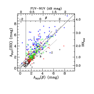
Figure 9: Bolometric versus colour-excess FUV extinctions for SFRS galaxies. Measured values of $\rm FUV-NUV$ GALEX colours and $\beta$ are shown on the upper axes. The abscissa is the resulting colour-excess extinction derived from the Seibert et al. (2005) relation. The ordinate is $A_{\rm FUV}(IRX)$ (Eq. 9, original source Buat et al., 2005); corresponding values of IRX_FUV are shown on the right. The solid line shows equality between the two $A_{\rm FUV}$ measures. The short-dashed diagonal line shows the empirical relation from Seibert et al. (2005), the long-dashed line shows the Kong et al. (2004) relation (which is almost the same as the Meurer et al. 1999 relation), the dotted line shows the Cortese et al. (2006) relation, and the dash-dot line shows the Casey et al. (2014) relation. Lines extend over the range of the respective samples. Point types show quartiles of 60 µm luminosity as indicated in the Figure 2 legend. The horizontal solid line indicates zero bolometric extinction, which occurs at $\log(\rm IRX)\approx-0.49$. The vertical solid line indicates $\beta=-1.5$, which corresponds to $A_{\rm FUV}(\beta)=1.05$.

An empirical expression for FUV extinction based on UV reddening of a diverse, UV-selected sample of 200 galaxies (Seibert et al., 2005) is

$$A_{\rm FUV}(\beta)=3.978(m_{\rm FUV}-m_{\rm NUV})+0.143~{}~{},$$ (10)

where $m_{\rm FUV}$ and $m_{\rm NUV}$ are the respective GALEX AB magnitudes. The equation is similar to relations derived by others (e.g., Hao et al., 2011). Figure 9 shows the SFRS galaxies in the IRX–$(m_{\rm FUV}-m_{\rm NUV})$ (or equivalently IRX–$\beta$) space. There is a correlation between $A_{\rm FUV}(\beta)$ and $A_{\rm FUV}({\rm IRX})$ with Pearson correlation coefficient $r=0.71$ and mean $\langle A_{\rm FUV}(\beta)-A_{\rm FUV}({\rm IRX})\rangle=0.33$ mag, but the rms scatter in $A_{\rm FUV}({\rm IRX})$ as derived from $A_{\rm FUV}(\beta)$ is 0.44 dex. Galaxies with $A_{\rm FUV}(\beta)\la 2$ can have bolometric extinctions as high as 6 mag, and $A_{\rm FUV}(\beta)$ applied to $L_{\rm FUV}$ greatly underestimates their FIR luminosity and therefore SFR. This is consistent with other results (e.g., Kong et al., 2004; Johnson et al., 2006, 2007), which have shown that galaxies having higher current SFR relative to their past averaged SFR are likely to deviate above the IRX–$\beta$ relation, i.e., have larger $A_{\rm FUV}({\rm IRX})$ for a given $A_{\rm FUV}(\beta)$. Despite this qualitative agreement, the Kong et al. mean numerical relation for their UV-selected sample of $50$ local starbursts is not a good fit to the FIR-selected SFRS data as shown in Figure 9. Regardless of numerical values, all these studies agree that galaxies with higher SFR are more obscured at fixed $\beta$ (also see Cortese et al., 2006; Moore et al., 2010; Iglesias-Páramo et al., 2004). At the low SFR end, galaxies with $L_{60}<10^{9.3}$ L_⊙, which at $z\approx 0$ are mostly early-type cluster galaxies, form two groups. Around 75 per cent of them are near the mean IRX–$\beta$ relation, but the rest show $A_{\rm FUV}({\rm IRX})\ll A_{\rm FUV}(\beta)$. One possibility is that these galaxies have older stellar populations with intrinsically high values of $\beta$. In the middle range $10^{9.3}<L_{60}<10^{10.7}$ L_⊙, there is a general trend for $A_{\rm FUV}({\rm IRX})$ to follow $A_{\rm FUV}(\beta)$ but with rms scatter $\sim$0.34 dex. At $L_{60}>10^{10.7}$ L_⊙, the scatter is $\sim$0.56 dex.

Some of the scatter in Figure 9 can be attributed to intrinsic dispersion in the SFHs and metallicity of individual galaxies (Cortese et al., 2006; Kong et al., 2004; Johnson et al., 2007; Wilkins et al., 2012; Grasha et al., 2013). It is therefore not surprising that the best-fit relation between $A_{\rm FUV}(\beta)$ and $A_{\rm FUV}({\rm IRX})$ matches well with the one derived for a UV-selected sample of galaxies with $IRAS$ counterparts (Seibert et al., 2005), similar to the SFRS sample used here, but is significantly different from the one proposed by Salim et al. (2007) for an optically-selected $z\sim 0.1$ sample of galaxies. Using a sample of galaxies from the SDSS and GALEX, Treyer et al. (2007) have also confirmed that UV-based extinction corrections (Seibert et al., 2005; Salim et al., 2007; Johnson et al., 2007) over (under) estimate the corrected UV luminosity for the lowest (highest) emission-line SFR galaxies. In that context, it is remarkable that Casey et al. (2014) found qualitatively the same results we do despite having selected 5/6 of their sample galaxies in the UV. (The other 1/6 of their sample was selected in the FIR, but most of those galaxies have $\mbox{$L_{\rm FIR}$}>10^{11}$ L_⊙.) The similarity of our results implies that they are not strongly biased by sample selection.

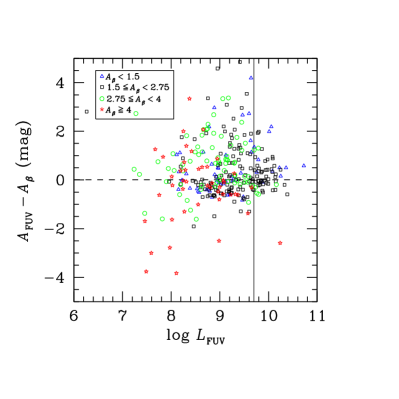
Figure 10: Difference between bolometric extinction $A_{\rm FUV}({\rm IRX})$ and colour-excess extinction $A_{\rm FUV}(\beta)$ as a function of observed FUV luminosity. Point types indicate $A_{\rm FUV}(\beta)$ as indicated in the legend. Dashed line indicates equality of the two extinction measures, i.e., for galaxies near the line, $A_{\rm FUV}(\beta)$ is a good predictor of $A_{\rm FUV}$ and therefore of SFR. The solid line marks $L_{\rm FUV}=5\times 10^{9}$ L_⊙.

The geometry of dust and stars in a galaxy is a crucial element in determining the attenuation at any given wavelength. However, while the relation between FUV attenuation and IRX is almost independent of dust geometry (Witt & Gordon, 2000), the relation between $\beta$ and IRX depends strongly on geometry of stars, gas, and dust (probably the main effect according to Casey et al. 2014), on dust grain properties, and on dust clumpiness (Witt & Gordon, 2000; Charlot & Fall, 2000; Meurer et al., 1999). For example, if young stars and dust are well mixed in an optically thick cloud, the extinction is high, but the UV light will emerge only from a layer near the surface and will show small $\beta$. Small $\beta$ can also be seen if our line of sight happens to pass through a low-extinction ‘tunnel’ to the young stars while their light emitted in other lines of sight is mostly absorbed. These considerations probably explain much of the scatter in using $\beta$ as an extinction indicator (Figure 9). Figure 10 further illustrates the problem of using UV data alone to estimate SFR. Ignorance of the actual FIR emission gives a median (mean) error in SFR of 0.22 (0.34) dex and maximum error 1.9 dex. There is no obvious way to know which galaxies will have deviant SFRs, though there are some clues. For 62 galaxies with $L_{\rm FUV}>5\times 10^{9}$ L_⊙ (and excluding two Seyfert galaxies SFRS 263/270—Maragkoudakis et al. 2018), the median deviation is 0.16 dex, and the maximum is 0.87 dex. Similarly, for 20 galaxies with $\beta<-1.5$ (or equivalently $A_{\rm FUV}(\beta)<1.05$ mag, the median deviation is 0.15 dex, and only one galaxy deviates by more than 0.4 dex (though the deviation for that galaxy is 1.7 dex). Thus for $\sim$1/4 of the SFRS sample and presumably a larger fraction of UV-selected samples, FIR estimates based on UV data are not bad. For the other $\sim$3/4 of the galaxies, however, the median deviation is 0.26 dex, and 28 per cent of the galaxies show deviations $>$0.5 dex.

In retrospect, it should not be surprising that $A_{\rm FUV}(\beta)$ gives a reasonable estimate of $A_{\rm FUV}$ when $A_{\rm FUV}(\beta)$ is small enough. When $A_{\rm FUV}<1$ mag, of order half or more of the UV light escapes, and the UV colour can indicate extinction. When extinction is larger, however, little light from stars suffering high absorption escapes. The light that does escape comes only from stars in lines of sight that have low absorption, and only this low extinction is measured. Figure 11(a) of Charlot & Fall (2000) illustrates the effect for a simple mixed-slab model. Real galaxies are even more complicated: Goldader et al. (2002) showed that the emerging UV light is often displaced from the main luminosity sources. Figure 1 shows some striking examples in the SFRS sample. Under these conditions, the colour of the emerging light cannot indicate whether there are many or few stars hidden by dust.

Another colour-excess extinction measure is the Balmer decrement, the H$\alpha$/H$\beta$ flux ratio measured spectroscopically. Maragkoudakis et al. (2018) gave nuclear Balmer decrements for the SFRS sample, most coming from SDSS fiber spectra. However, H$\alpha$/H$\beta$ used here has an inherent bias because the line ratio was measured from apertures 3″–3.5″ in diameter centred on each galaxy’s nucleus. This introduces biases in two ways:
(i) galaxies must have significant Balmer emission and therefore high nuclear star formation activity in order for emission lines to be measureable, and
(ii) the circumnuclear regions of galaxies are dustier than the outer disc (e.g., Popescu et al., 2005; Prescott et al., 2007), and hence for the nearby galaxies in the SFRS sample the nuclear obscuration could exceed the galaxy’s average value. Therefore, the results are only a rough indicator of the bolometric $A_{\rm FUV}$. A full analysis requires optical spectra covering a larger fraction of the galaxies’ areas (e.g., Cortese et al., 2006).

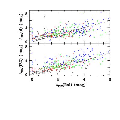
Figure 11: Measures of FUV extinction as a function of observed Balmer decrement. (Top) FUV colour-excess extinction $A_{\rm FUV}(\beta)$ (Eq. 10). (bottom) FUV bolometric extinction $A_{\rm FUV}({\rm IRX})$ (Eq. 9). Abscissa comes from Eq. 12. Point types indicate quartiles of 60 µm luminosity as indicated in the Figure 2 legend, and the dashed lines mark equal values of extinction on both axes.

To compute the FUV extinction implied by the Balmer decrements, we followed Domínguez et al. (2013):

$$E(B-V)=1.97\,\rm log\bigg{[}\frac{(H\alpha/H\beta)_{obs}}{2.86}\bigg{]}$$ (11)

where (H$\alpha$/H$\beta$)_obs is the observed Balmer decrement. The adopted reddening curve (Calzetti et al., 2000) translates the Equation 11 colour excess to

$$A_{\rm FUV}({\rm Bal})=10.27\cdot 0.44\cdot E(B-V)\quad,$$ (12)

where the factor 0.44 accounts for lower extinction to stars than to ionized gas. Figure 11 compares $A_{\rm FUV}(\rm Bal)$ with other extinction measures for the SFRS galaxies. $A_{\rm FUV}(\rm Bal)$ is correlated with $A_{\rm FUV}({\rm IRX})$, but the scatter is 0.60 dex rms. Galaxies with $L_{60}>10^{10.5}$ L_⊙ have even more scatter, 0.66 dex. For galaxies with $L_{60}<10^{10.5}$ L_⊙, the scatter is 0.51 dex, and $A_{\rm FUV}(\rm Bal)$ overestimates $A_{\rm FUV}({\rm IRX})$ (and hence SFR) by a median of 0.12 dex. Using a factor of 0.40 insted of 0.44 for the ratio of stellar to gas extinction increases the median overestimate to 0.17 dex but decreases the rms scatter to 0.48 dex. A factor of 0.48 gives median overestimate 0.04 dex but increases the scatter to 0.55 dex. These values represent a plausible range, but no fixed ratio will make the nuclear Balmer decrement a good predictor of $A_{\rm FUV}({\rm IRX})$. $A_{\rm FUV}(\beta)$ does a little better: for the whole sample, the scatter between $A_{\rm FUV}(\beta)$ and $A_{\rm FUV}({\rm IRX})$ is 0.49 dex and only 0.37 dex when $L_{60}<10^{10.5}$ L_⊙. Despite that, the averages of the estimates agree reasonably well: $A_{\rm FUV}(\beta)$ underestimates $A_{\rm FUV}({\rm IRX})$ by 0.15 dex for the whole sample and overestimates by 0.03 dex for $L_{60}<10^{10.5}$ L_⊙. There is little correlation between $A_{\rm FUV}(\rm Bal)$ and $A_{\rm FUV}(\beta)$, which relation shows rms scatter 0.63 dex. These results are in broad agreement with Wijesinghe et al. (2011), who used multi-wavelength data for a volume-limited sample of nearby galaxies to show that there is a stronger correlation between $\beta$ and IRX than between H$\alpha$/H$\beta$ and IRX but with a large scatter in both (Figures 9 and 11). Some of the scatter seen in Figure 11 may be attributed to the fact that $\beta$ depends not only on the distribution of dust and young stars but also on the age of that stellar population (Grasha et al., 2013), the contribution from older stellar populations, metallicity, and the slope of the IMF.

The inability of reddening based on H$\alpha$/H$\beta$ to correct $L_{\rm FUV}$ in a way that determines FIR luminosity has previously been reported by several authors (e.g., Wang & Heckman, 1996; Buat et al., 1999, 2002). In particular, Buat et al. (2002) showed that the correlation between dust extinction and $L_{\rm FIR}$ is weak but gets worse for $B$-band, H$\alpha$, or UV luminosities. While colour-excess extinction corrections may yield statistically useful SFRs for normal galaxies, especially for low-dust samples selected at blue wavelengths, identifying which galaxies are $L_{\rm FIR}\gtrsim 10^{10.5}$ L_⊙ starburst galaxies requires data at longer wavelengths.

5 Comparison with previous results

Using a heterogeneous sample of 249 galaxies from the literature, Bell (2003) presented a study similar to the present one. Our data confirm Bell’s principal conclusion: while FIR reliably represents the star formation in ${\sim}L^{*}$ galaxies, it represents only a fraction of it in lower-luminosity (${\sim}$0.01 L^∗) galaxies. Another of Bell (2003)’s suggestions was that radio emission also underestimates the SFR in low-luminosity galaxies, and that these corresponding underestimates are responsible for the observed FIR–radio correlation. Figure 3 confirms that result and Bell’s inference that the observed linear radio–FIR correlation is a coincidence of both indicators underestimating the SFR at low luminosities. The remedy is a non-linear relation between $L_{\rm 1.4GHz}$ and SFR, as suggested by Davies et al. (2017) and shown in Equation 3.

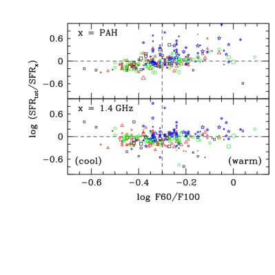
Figure 12: SFR_FIR relative to two other SFR measures as a function of dust temperature. The ratios on the ordinates are SFR_PAH (upper) and non-linear SFR2${}_{\rm 1.4\,GHz}$ (lower). The abscissa is the ratio of IRAS 60 to 100 µm flux densities. Symbol areas are proportional to weights in the SFRS sample (Paper I), and galaxies with $\rm weight<3$ (galaxies with uncommon properties) are not shown. Point types indicate quartiles of 60 µm luminosity as indicated in the Figure 2 legend. Horizontal dashed lines show equality, and the vertical dashed line marks $F_{60}/F_{100}=0.5$.

Bell (2003) also suggested a correlation between FIR dust temperature $T_{d}$ and $\eta$. In their picture, hotter dust would imply that active star formation is more important for dust heating, i.e., $\eta$ is smaller. Indeed, galaxies with $F_{60}/F_{100}>0.5$ are generally termed starbursts (Rowan-Robinson & Crawford, 1989), and 146 of our sample galaxies fit this criterion. However, as shown in Figure 12, contrary to the expectation, SFR_tot/SFR2${}_{\rm 1.4\,GHz}$ shows no correlation with $T_{d}$, and SFR_tot/SFR_PAH shows if anything an opposite correlation. That is, if cool dust were being heated by an old stellar population, SFR_tot would over-estimate SFR, contrary to the trend seen.

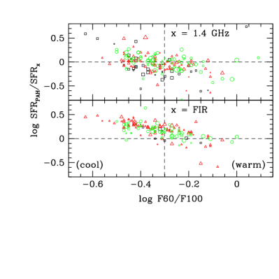
Figure 13: Ratio of SFR_FIR to SFR_PAH as a function of dust temperature. The abscissa is the ratio of IRAS 60 to 100 µm flux densities. Point areas are proportional to weights in the SFRS sample (Paper I), and points with $\rm weight<3$ are not shown. Point types indicate quartiles of 60 µm luminosity as indicated in the Figure 2 legend. The horizontal dashed line shows equality, and the vertical dashed line marks $F_{60}/F_{100}=0.5$. Points in the highest quartile of $L_{60}$ are omitted because SFR_PAH has large scatter for them as shown in Figs. 5 and 12.

The trend in SFR_tot/SFR_PAH in Figure 12 hints that $T_{d}$ may have some relation to PAH emission. That is confirmed by Figure 13, which shows that relative SFR_PAH is anti-correlated with $T_{d}$. The strongest negative correlation is with SFR_FIR, but the unweighted SFRS sample does not show a correlation of SFR_FIR with $T_{d}$ because the SFRS was constructed to cover the full range of $T_{d}$ uniformly at each value of $L_{\rm FIR}$. SFR_FIRwould correlate with $T_{d}$ for the SFRS if the galaxies were properly weighted. Numerous studies have shown associations between high SFR, high sSFR, high sSFR relative to the galaxy main sequence (‘starburstiness’), warm $T_{d}$, and low PAH emission (e.g., Elbaz et al., 2011; Nordon et al., 2012; Díaz-Santos et al., 2013; Stierwalt et al., 2014). What the SFRS sample shows is that at fixed $L_{\rm FIR}$ (or SFR), higher $T_{d}$ is associated with relatively smaller $L_{\rm PAH}$. We suggest that warm dust is associated with a relative deficiency of photo-dissociation regions, where the PAH emission originates. The most straightforward physical reason is high dust content in H ii regions of some galaxies. Such dust grains, being relatively near the heating sources, would reach relatively high temperatures, and the energy they absorb could not escape to excite PAH molecules in surrounding PDRs. This mechanism was suggested (Murata et al., 2014) to explain the PAH deficit in galaxies with high sSFR relative to their stellar masses. Whether this explanation is correct could perhaps be elucidated by spatially resolved observations.

Davies et al. (2017) used galaxies from the GAMA survey to derive conversions (linear and non-linear) from $L_{\rm 1.4\,GHz}$ to SFR. These authors found a non-linear relation with slope 0.66 and 0.4 dex scatter between $L_{\rm 1.4\,GHz}$ and their calculation of SFR_tot. For the SFRS sample, the scatter between SFR2${}_{\rm 1.4\,GHz}$ and our SFR_tot is only 0.25 dex. The SFRS data prefer a steeper slope $\sim$0.72 of the SFR–$L_{\rm 1.4\,GHz}$ relation, nearly equal to the slope of 0.75 found by Davies et al. using the MAGPHYS (da Cunha, Charlot, & Elbaz, 2008) estimate of SFR instead of their SFR_tot.

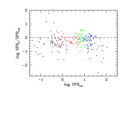
Figure 14: Ratio of $u$-band SFR (Hopkins et al., 2003, Eq. B8) to SFR_tot. Point types indicate quartiles of 60 µm luminosity as indicated in the Figure 2 legend, and the dashed line shows equality between the two measures. SFRS 17 (=NGC 2552) is omitted because it is very faint at $u=22.581$ mag.

Another common SFR indicator is the ground-based $u$-band (${\sim}3500$ Å in SDSS and similar data sets) luminosity. Hopkins et al. (2003) used a sample of 3079 galaxies observed at 1.4 GHz by FIRST and by SDSS to compare SFR indicators based on H$\alpha$, [O ii], $u$-band (here denoted SFR_U), and FIR luminosities against SFR${}_{\rm 1.4\,GHz}$. A critical element of the Hopkins et al. SFR calculation (their Eq. B8) was the $u$-band extinction correction, which they derived from each galaxy’s Balmer decrement. Davies et al. (2016) used the same SFR_U metric (among 12 that they examined) in a sample of morphologically selected spiral galaxies ($0<z<0.13$) from the Galaxy and Mass Assembly (GAMA) survey (Driver et al., 2016). One key difference is that Davies et al. derived the $u$-band extinction from fitting each galaxy’s spectral energy distribution, and they also put in a correction, based on $u-g$ colour, for $u$-band radiation from older stars. Figure 14 compares SFR_U to SFR_tot for 218 SFRS galaxies where SDSS data are available. The derived values of SFR_U are a factor of two lower than SFR_tot on average, and the rms scatter is 0.6 dex. This applies even for low-luminosity galaxies, despite SFR_FUV often being dominant over SFR_FIR (Fig. 2). Correcting for $u$-band emission by old stars (Davies et al., 2016, Eq. 12) would make the discrepancy worse, increasing the median SFR_U deficit to 0.5 dex and the scatter to 0.67 dex. The systematic errors and large scatter make $u$-band luminosity an unreliable SFR indicator for galaxies with dust such as the SFRS sample.

Bell (2003) showed that the H$\alpha$ and FUV extinctions loosely correlate with each other, with the former being around half of the latter. Our observations (Figure 11) agree with the correlation, but neither indicator is a reliable measure of bolometric extinction (Figure 9). Wang et al. (2016) similarly studied a subsample of 745 galaxies from the GAMA and Herschel Astrophysical Terahertz Large Area Survey (H-ATLAS) to test correlations between multi-wavelength SFR tracers. Wang et al. (2016) derived SFRs using FIR, sub-mm, dust-corrected UV photometric data, and H$\alpha$ emission line luminosities, the last two corrected for attenuation using the Balmer decrement. Wang et al. found that UV data can be reconciled with the attenuation-corrected H$\alpha$ SFR and their version of SFR_tot (computed assuming $\eta=0.54$; Eq. 7) after applying an attenuation correction based on IRX. In agreement with our results, Wang et al. showed that the UV spectral slope $\beta$ is not a reliable attenuation indicator on its own. Wang et al. also found that the attenuation correction factor depends on stellar mass, redshift, and dust temperature but is independent of the H$\alpha$ equivalent width and Sérsic index. To summarize, none of the colour-excess indicators we have tested can be considered reliable for general galaxy samples.

6 Summary and prospects

The main conclusion of our work is that for local galaxies, global SFRs can be derived consistently from radio continuum, FIR+UV, or 8.0 µm PAH emission with scatter ${\la}0.3$ dex in SFR over four orders of magnitude in galaxy luminosity. In particular, the SFRS results confirm and quantify:

• For measuring SFR from 1.4 GHz radio observations, the preferred calibration is non-linear with a slope near the 0.75 value found also by Davies et al. (2017).

• The distributions of SFR_tot, non-linear SFR2${}_{\rm 1.4\,GHz}$, and SFR_PAH show similar statistical properties. We have presented mutually consistent (within 5 per cent) calibrations for these measures of SFR.

• $L_{\rm FIR}$ captures most of the emergent luminosity for most luminous ($\log L_{60}\geq 10.5$ L_⊙) galaxies and is therefore a good measure of their SFR. Lower-luminosity galaxies tend to have more of their emission in the UV, which is therefore needed to estimate their SFR. Different numerical prescriptions, such as adding SFR_FUV or SFR_NUV or using a bolometric extinction correction for the UV light, give statistically similar results.

• SFR estimates obtained from UV data alone are subject to large uncertainties in the extinction corrections. At fixed UV colour or spectral slope $\beta$, galaxies with $L_{\rm FUV}<5\times 10^{9}$ L_⊙ show a broad range in $A_{\rm FUV}$. Therefore the UV spectral slope is not a good measure of the correction needed, and extinction corrections based on UV colour may yield SFR_FUV differing from the total SFR by up to 2 dex. In contrast, for galaxies with $L_{\rm FUV}>5\times 10^{9}$ L_⊙ or $\beta<-1.5$, $L_{\rm FUV}$ corrected by extinction based on UV spectral slope ($A_{\rm FUV}(\beta)$) can measure SFR with rms scatter $\sim$0.24 dex.

The SFRS data also reveal:

• For galaxies with ${\rm FUV}-[3.6]\la 2$, PAH luminosity underestimates SFR by up to $\sim$1 dex.

• The FIR-selected SFRS sample shows a surprising preference for $\eta=0$ for obtaining SFR_tot. In other words, when using $L_{\rm FIR}$ to deduce SFR, accounting for dust heating by an older stellar population unrelated to current star formation is unimportant. The existence of the star-forming-galaxy main sequence and the sub-galactic main sequence (Maragkoudakis et al., 2017, and references therein) suggests that at least part of the explanation is the close association between current star formation and the pre-existing stellar population. Much larger samples or better theoretical understanding of the SFR tracers will be needed for accurate measurements of $\eta$.

• Dust temperature does not correlate with most measures of SFR, but there is a close relation between dust temperature and SFR_PAH/SFR_FIR. This needs to be explored in spatially resolved galaxies.

Consistency of various SFR indicators does not prove they are correct. Some authors (e.g., Boquien, Buat, & Perret, 2014; da Silva, Fumagalli, & Krumholz, 2014) have suggested that bursty star formation histories can cause measured SFRs to deviate from the true values. We have not examined that suggestion because the purpose of this paper is to inter-compare empirical SFR indicators, but future work should investigate this possibility. Future work should also include better decomposition of the SFRS galaxies into AGN and star-forming components and the correlations of SFR indicators with each component. Additional SFR indicators such as H$\alpha$ line flux, full SED fitting with derivation of reddening and corrected UV flux, and Spitzer/MIPS 24 µm or WISE 25 µm should also be examined.

Table A6: GALEX data for SFRS galaxies

SFRSa	Name	$D$(Mpc)a	FUVb	$\Delta$FUV	NUVb	$\Delta$NUV	$E(B-V)$c
1	IC 486	114.4	18.179	0.029	17.575	0.014	0.040
2	IC 2217	76.1	16.434	0.013	15.939	0.006	0.041
3	NGC 2500	15.0	13.925	0.004	13.785	0.002	0.040
5	MCG 6-18-009	164.4	17.890	0.026	17.064	0.011	0.052
8	NGC 2532	77.6	15.417	0.008	14.862	0.004	0.054
9	UGC 4261	93.2	16.485	0.014	16.159	0.007	0.055
10	NGC 2535	61.6	15.708	0.010	15.290	0.004	0.043
11	NGC 2543	26.3	15.986	0.011	15.516	0.005	0.069
12	NGC 2537	15.0	14.964	0.007	14.752	0.003	0.054
13	IC 2233	13.7	15.000	0.007	14.805	0.004	0.052
14	IC 2239	88.5	19.177	0.046	18.041	0.016	0.053
15	UGC 4286	75.1	17.372	0.020	16.945	0.009	0.047
16	UGC 4306	36.0	18.679	0.036	18.131	0.019	0.069
17	NGC 2552	11.4	14.736	0.006	14.587	0.003	0.047
18	IC 2339	79.3	17.100	0.018	16.702	0.009	0.047
19	IRAS 08234+1054	272.6	19.653	0.055	18.961	0.028	0.050
20	IRAS 08269+1514	134.5	20.736	0.074	19.758	0.028	0.033
21	NGC 2604	36.3	15.008	0.007	14.506	0.003	0.041
22	NGC 2608	36.3	16.004	0.011	15.414	0.006	0.039
24	NGC 2623	81.6	17.512	0.022	16.861	0.009	0.041
25	CGCG 120-018	107.9	20.649	0.078	19.397	0.026	0.034
29	IRAS 08512+2727	265.3	18.413	0.032	17.805	0.014	0.034
31	IRAS 08538+4256	121.2	19.898	0.062	18.661	0.022	0.024
32	IRAS 08550+3908	367.8	19.943	0.063	19.615	0.032	0.029
33	NGC 2718	57.4	15.772	0.010	15.298	0.005	0.071
34	NGC 2712	30.9	15.372	0.008	15.045	0.004	0.020
35	NGC 2719	51.1	16.235	0.012	15.759	0.005	0.033
36	IRAS 08572+3915NW	244.3	20.653	0.054	20.212	0.026	0.027
37	IRAS 08579+3447	273.5	19.027	0.042	18.260	0.017	0.028
38	NGC 2731	35.0	16.621	0.014	16.099	0.007	0.065
39	NGC 2730	58.9	15.753	0.010	15.390	0.005	0.027
40	IC 2431	209.0	18.787	0.038	18.173	0.017	0.050
41	NGC 2750	37.0	14.993	0.007	14.637	0.004	0.036
42	IC 2434	104.5	17.590	0.022	17.041	0.010	0.020
43	NGC 2761	125.0	18.753	0.037	17.851	0.014	0.036
44	NGC 2773	80.4	18.353	0.031	17.646	0.013	0.048
45	NGC 2776	36.0	14.520	0.006	14.089	0.003	0.014
46	NGC 2789	93.6	18.281	0.031	17.218	0.011	0.026
48	NGC 2824	42.5	19.236	0.047	17.950	0.015	0.032
49	IRAS 09184+4356	170.1	20.281	0.073	19.564	0.032	0.015
50	CGCG 238-041	131.5	18.122	0.022	17.627	0.010	0.015
51	UGC 4985	143.4	19.735	0.057	19.442	0.033	0.036
52	NGC 2854	25.0	16.742	0.015	16.210	0.007	0.018
53	UGC 5046	64.9	17.862	0.025	17.020	0.010	0.034
54	UGC 5055	110.6	16.568	0.014	16.112	0.007	0.034
55	NGC 2893	24.0	16.229	0.012	15.674	0.005	0.023
56	MCG 3-24-062	66.3	18.404	0.032	18.130	0.017	0.045
57	CGCG 238-066	147.0	19.008	0.042	18.281	0.018	0.012
58	UGC 5097	72.5	16.210	0.012	15.841	0.006	0.039
59	CGCG 289-012	172.5	17.394	0.020	16.948	0.009	0.020
60	MCG 8-18-013	110.9	18.171	0.029	17.572	0.013	0.024
61	CGCG 181-068	100.6	20.206	0.070	19.396	0.032	0.014
62	NGC 2936	100.5	16.655	0.015	16.210	0.007	0.034
63	NGC 2955	103.5	16.395	0.013	15.853	0.006	0.011
64	CGCG 182-010	175.1	18.727	0.037	18.102	0.016	0.012
65	UGC 5228	28.2	16.937	0.017	16.440	0.009	0.164
67	NGC 3015	108.8	17.958	0.026	17.232	0.011	0.084
68	MCG 2-25-039	77.6	18.050	0.027	17.468	0.012	0.031
69	NGC 3020	18.3	14.492	0.005	14.200	0.003	0.038
70	NGC 3049	18.3	15.477	0.009	15.122	0.004	0.038
71	NGC 3055	25.0	15.203	0.008	14.744	0.004	0.052
72	IC 2520	26.4	16.496	0.014	16.171	0.007	0.021
73	UGC 5403	33.0	18.118	0.028	17.502	0.012	0.031
74	UGC 5459	25.8	15.529	0.009	14.508	0.003	0.007
75	MCG 5-24-022	92.1	19.488	0.150	18.203	0.016	0.022
76	IC 2551	94.9	17.990	0.027	17.004	0.010	0.036
77	IRAS 10106+2745	215.6	21.136	0.087	19.952	0.030	0.054
78	NGC 3162	26.4	14.479	0.005	14.129	0.003	0.023
79	IRAS 10120+1653	517.2	23.088	0.158	21.807	0.069	0.036
80	NGC 3190	26.4	17.508	0.022	16.277	0.007	0.025
81	IC 602	57.6	15.492	0.009	15.184	0.004	0.026
82	NGC 3191	134.0	16.243	0.012	15.834	0.006	0.012
83	NGC 3206	25.8	14.391	0.005	14.098	0.003	0.014
84	UGC 5613	139.8	17.585	0.022	16.605	0.008	0.014
85	UGC 5644	137.6	17.328	0.020	16.889	0.010	0.042
86	NGC 3245	20.9	17.745	0.024	16.343	0.009	0.025
88	MCG 7-22-012	66.0	18.827	0.039	18.130	0.016	0.011
89	IRAS 10276+1119	271.3	18.174	0.029	17.905	0.015	0.033
90	NGC 3265	21.8	17.273	0.019	16.784	0.009	0.024
91	UGC 5713	95.0	18.375	0.032	18.009	0.018	0.019
93	UGC 5720	20.0	15.071	0.007	14.831	0.004	0.012
92	NGC 3274	10.0	14.687	0.006	14.479	0.003	0.024
95	NGC 3306	46.6	16.448	0.013	16.073	0.006	0.025
96	NGC 3323	79.5	16.081	0.011	15.677	0.005	0.024
97	IC 2598	89.1	18.408	0.032	17.619	0.013	0.029
98	NGC 3338	21.4	14.300	0.005	13.847	0.003	0.031
99	NGC 3353	16.0	14.868	0.006	14.667	0.003	0.007
100	UGC 5881	93.0	18.495	0.033	17.688	0.014	0.030
101	NGC 3370	20.9	14.845	0.006	14.441	0.003	0.031
102	NGC 3381	25.7	15.116	0.007	14.728	0.004	0.020
103	UGC 5941	107.0	19.109	0.044	17.918	0.015	0.012
104	NGC 3413	16.2	15.493	0.009	15.109	0.004	0.023
105	NGC 3408	138.0	16.989	0.017	16.448	0.007	0.012
106	NGC 3430	28.4	20.146	0.069	19.361	0.028	0.024
107	CGCG 95-055	25.7	14.602	0.006	14.168	0.003	0.031
109	UGC 6074	38.0	18.289	0.031	17.441	0.012	0.015
110	NGC 3495	17.5	15.291	0.008	14.726	0.004	0.046
111	UGC 6103	91.7	16.208	0.012	15.676	0.005	0.009
112	MCG 7-23-019	150.6	17.344	0.020	16.920	0.009	0.009
113	UGC 6135	90.9	16.551	0.014	15.941	0.006	0.008
114	CGCG 241-078	110.9	20.440	0.215	19.183	0.025	0.009
115	IRAS 11069+2711	296.4	19.304	0.036	19.241	0.021	0.021
116	IC 676	26.9	17.796	0.025	16.839	0.009	0.025
117	IRAS 11102+3026	129.6	22.427	0.135	20.895	0.042	0.021
118	IC 2637	128.2	17.409	0.021	16.695	0.008	0.022
119	MCG 9-19-013	201.8	19.958	0.063	19.265	0.028	0.016
120	7Zw 384	340.4	18.649	0.028	18.004	0.012	0.008
121	IRAS 11167+5351	447.3	20.357	0.053	20.003	0.027	0.014
122	NGC 3633	30.0	18.619	0.036	17.779	0.014	0.062
124	NGC 3656	37.0	17.272	0.020	16.487	0.008	0.015
126	NGC 3664	26.9	14.685	0.006	14.441	0.003	0.045
127	NGC 3666	16.3	15.532	0.009	15.020	0.004	0.033
128	IC 691	16.0	16.560	0.014	16.251	0.007	0.014
129	NGC 3686	21.0	14.432	0.005	13.890	0.003	0.024
130	UGC 6469	102.6	16.334	0.013	15.909	0.006	0.037
131	NGC 3690	52.6	15.996	0.008	15.511	0.004	0.017
132	IC 698	96.8	18.445	0.033	17.421	0.013	0.043
133	IRAS 11267+1558	736.6	22.046	0.090	21.665	0.045	0.045
134	NGC 3705	16.3	15.009	0.007	14.517	0.003	0.046
135	MCG 3-29-061	67.5	18.785	0.038	18.054	0.016	0.022
136	NGC 3720	89.8	16.934	0.012	15.922	0.005	0.029
137	NGC 3729	17.1	15.626	0.009	15.068	0.004	0.011
139	NGC 3758	131.6	17.700	0.023	16.834	0.020	0.025
140	UGC 6583	93.2	16.851	0.016	16.291	0.007	0.026
142	NGC 3769	17.1	15.163	0.007	14.752	0.003	0.023
143	NGC 3773	16.3	15.240	0.008	14.963	0.004	0.027
144	NGC 3781	103.5	20.374	0.076	18.764	0.021	0.026
145	UGC 6625	158.2	16.260	0.012	15.778	0.005	0.026
146	NGC 3808	107.2	18.376	0.032	17.644	0.013	0.026
148	NGC 3822	94.6	17.915	0.026	16.914	0.009	0.056
149	UGC 6665	85.0	15.735	0.010	15.322	0.004	0.025
150	MCG 3-30-051	90.4	17.574	0.022	17.173	0.010	0.020
152	UGC 6732	53.6	19.415	0.050	17.479	0.012	0.020
153	IC 730	93.1	18.778	0.038	18.039	0.015	0.021
155	NGC 3912	22.5	16.286	0.012	15.621	0.005	0.021
156	NGC 3928	16.9	15.658	0.009	15.220	0.004	0.020
157	NGC 3934	61.6	19.687	0.059	18.745	0.023	0.055
158	UGC 6865	91.2	18.342	0.031	17.340	0.011	0.020
159	UGC 6901	107.6	18.684	0.036	17.456	0.012	0.015
160	CGCG 013-010	172.3	19.818	0.060	18.646	0.023	0.016
161	NGC 3991	55.6	14.581	0.006	14.449	0.003	0.022
162	NGC 4004	57.9	15.813	0.010	15.454	0.005	0.025
163	NGC 4014	62.6	17.129	0.018	16.448	0.008	0.065
164	NGC 4010	17.1	16.142	0.012	15.608	0.005	0.025
165	NGC 4018	72.6	18.075	0.028	17.290	0.011	0.021
166	NGC 4020	14.3	15.458	0.009	15.122	0.004	0.017
167	IRAS 11571+3003	218.6	21.136	0.095	20.257	0.038	0.018
169	UGC 7016	110.3	18.982	0.042	17.906	0.016	0.038
168	UGC 7017	55.3	16.731	0.015	16.387	0.007	0.019
170	MCG 3-31-030	13.1	16.820	0.016	16.406	0.007	0.030
171	NGC 4062	16.3	14.937	0.007	14.360	0.003	0.025
172	NGC 4064	8.5	17.034	0.018	15.889	0.006	0.021
173	CGCG 098-059	102.3	19.226	0.046	18.020	0.017	0.049
174	NGC 4116	16.0	14.278	0.005	14.068	0.003	0.022
175	NGC 4136	16.3	14.049	0.005	13.741	0.003	0.018
176	NGC 4150	13.7	17.726	0.024	16.326	0.007	0.018
177	IRAS 12086+1441	13.1	21.100	0.068	20.507	0.032	0.036
178	NGC 4162	42.5	15.549	0.009	14.938	0.004	0.035
179	NGC 4178	16.8	14.115	0.005	13.734	0.002	0.028
181	NGC 4189	16.8	15.325	0.008	14.798	0.004	0.033
183	NGC 4204	10.0	15.188	0.008	14.946	0.004	0.034
184	NGC 4207	16.8	17.284	0.019	16.604	0.008	0.017
185	UGC 7286	115.4	19.081	0.043	18.184	0.016	0.020
186	NGC 4234	30.0	15.426	0.008	15.011	0.004	0.018
187	NGC 4237	16.8	16.249	0.012	15.316	0.005	0.030
188	NGC 4244	4.3	13.045	0.003	12.546	0.001	0.021
189	NGC 4253	64.9	17.589	0.022	16.839	0.009	0.020
190	MCG 3-32-005	13.1	18.598	0.035	17.720	0.013	0.028
191	NGC 4290	37.0	15.859	0.027	15.346	0.005	0.014
192	NGC 4294	16.8	14.544	0.006	14.165	0.003	0.034
193	NGC 4314	16.3	15.848	0.010	14.951	0.004	0.025
194	NGC 4385	29.0	15.574	0.009	15.213	0.004	0.025
196	NGC 4396	16.8	15.137	0.007	14.790	0.004	0.026
197	NGC 4412	30.6	15.367	0.008	14.971	0.004	0.018
199	NGC 4420	17.6	15.005	0.007	14.484	0.003	0.018
200	NGC 4424	6.0	16.296	0.013	15.418	0.005	0.021
201	NGC 4435	16.7	18.515	0.035	16.763	0.009	0.030
202	NGC 4438	16.8	15.844	0.010	15.241	0.004	0.028
203	NGC 4448	16.3	16.310	0.013	15.585	0.006	0.024
205	NGC 4470	16.8	15.238	0.008	14.868	0.004	0.024
207	NGC 4491	16.8	17.596	0.023	16.903	0.009	0.042
209	NGC 4495	74.2	17.244	0.019	16.646	0.008	0.021
210	IC 3476	16.8	15.077	0.007	14.497	0.003	0.036
211	NGC 4509	11.1	15.412	0.008	15.238	0.004	0.012
212	NGC 4519	16.8	14.309	0.005	13.955	0.002	0.020
213	NGC 4548	16.2	14.973	0.007	14.462	0.003	0.038
214	IRAS 12337+5044	172.5	18.230	0.073	17.693	0.013	0.012
216	NGC 4592	11.1	14.177	0.005	13.840	0.003	0.022
217	NGC 4607	16.8	17.943	0.027	17.202	0.011	0.032
218	NGC 4625	9.2	15.283	0.008	14.986	0.004	0.018
219	NGC 4630	15.6	15.493	0.009	15.123	0.004	0.030
222	MCG 5-30-069	74.0	20.277	0.073	18.822	0.022	0.015
223	IC 3721	98.5	17.723	0.024	17.014	0.010	0.019
224	NGC 4670	14.3	14.313	0.005	14.115	0.003	0.015
226	MCG 7-26-051	146.9	19.704	0.057	18.889	0.024	0.022
228	NGC 4688	15.6	14.740	0.006	14.625	0.004	0.031
229	NGC 4704	122.8	16.979	0.017	16.555	0.008	0.017
231	IRAS 12468+3436	498.3	24.890	0.281	22.798	0.075	0.014
233	MCG 8-23-097	131.2	19.748	0.058	18.866	0.023	0.013
234	NGC 4747	14.3	16.444	0.013	16.179	0.008	0.010
235	UGC 8017	107.1	17.548	0.022	17.087	0.010	0.010
236	NGC 4765	15.6	15.199	0.008	14.776	0.004	0.040
237	VCC2096	13.1	18.511	0.033	17.828	0.014	0.051
238	UGC 8041	23.0	14.962	0.007	14.636	0.003	0.022
240	NGC 4837	132.5	16.658	0.015	16.204	0.007	0.014
241	UM530	282.7	18.851	0.027	18.506	0.013	0.021
242	NGC 4861	18.5	14.628	0.006	14.430	0.003	0.010
244	NGC 4922	107.2	19.225	0.046	18.509	0.019	0.011
245	UGC 8179	222.1	17.509	0.022	17.152	0.011	0.013
246	NGC 5001	134.8	18.223	0.030	17.100	0.010	0.016
247	IC 856	64.3	17.795	0.024	17.235	0.010	0.035
248	UGC 8269	124.1	20.814	0.091	19.745	0.034	0.012
250	NGC 5012	40.2	15.090	0.007	14.512	0.003	0.014
249	NGC 5014	18.5	16.779	0.015	16.143	0.007	0.008
251	IRAS 13116+4508	258.3	22.285	0.126	21.000	0.047	0.016
252	IC 860	54.5	20.272	0.306	18.316	0.019	0.013
253	IRAS 13144+4508	381.8	18.892	0.029	18.605	0.015	0.018
254	NGC 5060	97.4	17.122	0.018	16.433	0.007	0.034
255	UGC 8357	146.9	17.289	0.019	16.680	0.008	0.026
256	UGC 8361	106.3	18.921	0.040	18.137	0.016	0.038
257	IC 883	104.7	17.703	0.024	16.939	0.010	0.013
258	NGC 5100	142.2	18.101	0.028	17.289	0.011	0.029
259	NGC 5104	87.8	18.082	0.028	17.534	0.013	0.023
260	NGC 5107	18.5	15.420	0.008	15.063	0.004	0.011
262	NGC 5123	123.4	16.085	0.011	15.604	0.005	0.013
263	IRAS 13218+0552	850.44	20.564	0.049	21.164	0.037	0.031
264	IRAS 13232+1731	331.8	18.034	0.027	17.443	0.012	0.021
265	NGC 5147	18.0	14.293	0.005	13.938	0.002	0.027
266	NGC 5204	3.3	13.167	0.003	13.014	0.002	0.013
267	UGC 8502	149.9	15.943	0.010	15.709	0.005	0.011
268	UGC 8561	107.5	15.819	0.010	15.455	0.005	0.011
269	NGC 5230	105.6	15.235	0.008	14.753	0.003	0.025
270	IRAS 13349+2438	453.5	18.660	0.029	17.344	0.009	0.012
272	UGC 8626	108.8	17.820	0.025	17.193	0.010	0.028
271	NGC 5256	125.2	16.806	0.016	16.292	0.009	0.013
273	NGC 5263	77.5	16.838	0.016	16.394	0.007	0.013
274	MCG 1-35-028	105.1	18.506	0.034	17.683	0.014	0.030
275	IC 910	120.3	18.354	0.031	17.684	0.013	0.017
276	Mrk 268	173.7	19.024	0.042	18.390	0.018	0.016
277	NGC 5278	114.4	16.357	0.013	15.864	0.006	0.009
278	NGC 5273	16.5	17.496	0.022	16.620	0.009	0.010
279	UGC 8685	152.6	16.693	0.015	16.302	0.007	0.014
280	UGC 8686	105.4	17.119	0.018	16.884	0.009	0.026
281	UGC 8696	163.0	18.377	0.032	17.562	0.012	0.008
283	Mrk 796	98.5	18.253	0.023	17.494	0.010	0.026
282	NGC 5297	30.9	14.892	0.007	14.468	0.003	0.014
284	IRAS 13446+1121	104.6	20.637	0.085	19.222	0.029	0.035
285	NGC 5303	23.0	15.486	0.009	15.092	0.004	0.014
286	NGC 5313	30.9	15.799	0.010	15.240	0.004	0.008
287	MCG 3-35-034	178.6	19.052	0.043	18.283	0.018	0.023
288	NGC 5347	39.0	16.295	0.012	15.883	0.006	0.021
289	NGC 5350	30.9	14.834	0.006	14.541	0.003	0.011
291	UGC 8827	85.4	17.459	0.021	16.715	0.009	0.023
293	UGC 8856	137.9	18.939	0.040	18.398	0.019	0.016
294	NGC 5374	68.9	15.673	0.009	15.214	0.004	0.027
295	UGC 8902	114.4	16.935	0.017	16.423	0.008	0.022
296	NGC 5403	37.0	17.581	0.022	17.015	0.011	0.009
297	MCG 7-29-036	144.6	19.870	0.061	19.449	0.030	0.011
299	MCG 5-33-046	116.4	20.712	0.088	19.157	0.029	0.014
300	NGC 5474	5.6	14.318	0.005	14.191	0.003	0.011
302	MCG 6-31-070	155.8	18.301	0.103	18.040	0.016	0.016
303	CGCG 074-129	76.5	20.453	0.274	19.101	0.027	0.024
305	NGC 5515	114.1	17.681	0.023	16.830	0.009	0.008
304	NGC 5520	30.5	15.876	0.010	15.272	0.004	0.018
306	NGC 5526	27.9	17.716	0.024	16.861	0.009	0.012
307	NGC 5522	72.1	17.442	0.021	16.723	0.009	0.024
308	NGC 5541	115.4	16.548	0.014	15.914	0.006	0.011
309	IC 4395	160.5	17.640	0.023	16.684	0.008	0.017
310	UGC 9165	81.3	18.758	0.038	18.123	0.016	0.017
311	Mrk 1490	116.2	20.862	0.093	19.271	0.026	0.018
312	NGC 5585	5.6	13.318	0.003	13.142	0.002	0.016
313	IC 4408	134.9	18.451	0.033	17.681	0.013	0.021
314	NGC 5584	23.1	14.304	0.005	13.926	0.002	0.039
315	NGC 5633	36.5	15.711	0.010	15.130	0.004	0.017
316	NGC 5660	38.9	14.274	0.005	13.868	0.002	0.021
317	NGC 5656	53.7	15.916	0.011	15.337	0.005	0.015
318	NGC 5657	64.4	17.256	0.019	16.935	0.010	0.018
319	CGCG 133-083	190.6	19.039	0.042	18.354	0.017	0.048
320	MCG 7-30-028	116.1	17.796	0.024	17.330	0.011	0.012
321	MCG 6-32-070	127.1	17.141	0.018	16.332	0.007	0.010
322	UGC 9412	138.7	14.825	0.006	14.778	0.003	0.007
324	NGC 5691	19.8	15.272	0.008	14.797	0.004	0.037
325	MCG 9-24-035	137.4	19.059	0.043	17.988	0.017	0.022
326	MCG 9-24-038	166.6	19.254	0.046	18.422	0.018	0.016
327	UGC 9560	23.0	15.360	0.008	15.323	0.004	0.012
328	IC 1076	92.6	16.879	0.016	16.289	0.007	0.031
329	IRAS 14538+1730	432.9	21.043	0.101	19.689	0.032	0.027
330	NGC 5795	38.2	17.965	0.026	17.229	0.011	0.019
331	UGC 9618	145.8	19.178	0.045	18.582	0.019	0.042
332	UGC 9639	157.7	18.082	0.028	17.166	0.011	0.018
333	MCG 6-33-022	194.5	18.685	0.036	18.114	0.017	0.016
334	NGC 5879	15.5	14.598	0.006	14.289	0.003	0.012
335	MCG 9-25-036	160.1	20.680	0.073	19.776	0.029	0.018
336	NGC 5899	43.5	16.323	0.013	15.679	0.006	0.034
337	NGC 5905	58.7	15.358	0.008	15.155	0.005	0.015
338	Mrk 848	173.9	17.811	0.024	17.115	0.010	0.026
339	IC 4553	83.5	17.962	0.026	17.175	0.013	0.051
340	UGC 9922	86.7	16.585	0.014	16.325	0.007	0.017
341	IC 4567	88.6	16.502	0.014	15.888	0.006	0.029
342	MCG 4-37-016	102.9	17.952	0.026	17.238	0.011	0.047
343	NGC 5975	69.3	19.005	0.042	18.201	0.020	0.063
344	NGC 5980	65.2	16.422	0.013	15.844	0.006	0.035
345	NGC 5992	140.2	16.574	0.014	16.112	0.006	0.020
346	NGC 5996	54.0	14.836	0.006	14.475	0.003	0.034
347	IRAS 15519+3537	354.1	20.629	0.062	20.026	0.028	0.025
348	UGC 10099	152.2	16.371	0.013	16.034	0.006	0.018
349	MCG 5-38-006	69.6	18.674	0.036	17.973	0.015	0.051
351	NGC 6027A	70.6	20.475	0.081	19.600	0.031	0.055
350	UGC 10120	138.9	16.570	0.014	16.153	0.007	0.025
352	NGC 6040	177.0	17.108	0.018	16.715	0.010	0.044
353	UGC 10200	31.2	15.086	0.007	14.906	0.004	0.010
354	IRAS 16052+5334	366.1	22.846	0.154	21.821	0.060	0.012
355	IRAS 16053+1836	161.4	20.857	0.093	19.589	0.036	0.043
356	NGC 6090	131.2	16.472	0.013	15.871	0.006	0.020
357	UGC 10273	111.3	17.265	0.019	16.978	0.009	0.051
358	IRAS 16150+2233	278.1	21.368	0.092	20.510	0.043	0.112
359	UGC 10322	69.1	17.798	0.024	17.457	0.013	0.090
360	NGC 6120	134.9	17.360	0.020	16.749	0.009	0.018
361	MCG 3-42-004	171.9	18.171	0.029	17.619	0.014	0.066
362	UGC 10407	124.7	15.789	0.010	15.471	0.005	0.008
363	IRAS 16320+3922	139.4	17.012	0.017	16.610	0.008	0.010
364	NGC 6186	162.8	16.912	0.016	16.223	0.008	0.047
366	UGC 10514	100.5	17.248	0.019	16.882	0.009	0.051
367	IRAS 16435+2154	142.3	20.367	0.076	19.604	0.036	0.047
368	IC 4623	138.5	19.026	0.042	18.568	0.021	0.064
369	IRAS 16516+3030	306.1	21.397	0.085	20.554	0.037	0.034
aAshby et al. 2011; distances based on $H_{0}=73$ km s-1 Mpc-1
bAB magnitude
cMilky Way colour excess in magnitudes from Schlegel, Finkbeiner, & Davis (1998)

Table A7: SFR measures^a for SFRS galaxies

SFRSb	SFRFUV	SFRNUV	SFR${}_{\rm 1.4\,GHz}$	SFR2${}_{\rm 1.4\,GHz}$	SFRFIR	SFRPAH	SFRtotc
1	$-$0.18	0.06	0.97	0.87	0.57	0.74	0.64
2	0.16	0.36	0.89	0.81	0.65	0.84	0.78
3	$-$0.25	$-$0.19	$-$0.63	$-$0.33	$-$0.69	$-$0.53	$-$0.11
5	0.29	0.61	1.53	1.29	1.14	1.22	1.20
8	0.63	0.85	1.30	1.11	0.92	1.31	1.10
9	0.37	0.49	0.70	0.67	0.45	0.45	0.71
10	0.28	0.44	0.69	0.66	0.48	0.68	0.69
11	$-$0.49	$-$0.30	$-$0.22	$-$0.03	$-$0.19	0.03	$-$0.01
12	$-$0.62	$-$0.54	$-$0.78	$-$0.44	$-$0.66	$-$0.77	$-$0.34
13	$-$0.72	$-$0.64	$-$1.58	$-$1.04	$-$1.30	$-$1.77	$-$0.61
14	$-$0.76	$-$0.31	0.84	0.77	0.85	0.66	0.86
15	$-$0.20	$-$0.04	0.19	0.29	0.20	0.48	0.35
16	$-$1.29	$-$1.08	0.39	0.44	0.16	0.35	0.18
17	$-$0.79	$-$0.73	$-$2.44	$-$1.68	$-$1.56	$-$1.58	$-$0.72
18	$-$0.05	0.11	0.43	0.46	0.50	0.36	0.60
19	0.01	0.29	1.67	1.39	1.61	1.14	1.62
20	$-$1.09	$-$0.70	0.92	0.83	0.74	0.71	0.75
21	0.09	0.29	$-$0.06	0.10	$-$0.24	$-$0.09	0.26
22	$-$0.31	$-$0.08	0.15	0.25	0.04	0.31	0.20
24	$-$0.21	0.05	1.65	1.38	1.63	1.02	1.63
25	$-$1.24	$-$0.74	1.00	0.90	1.01	0.81	1.02
29	0.43	0.67	1.60	1.35	1.24	1.48	1.30
31	$-$0.87	$-$0.38	1.34	1.15	1.28	0.86	1.28
32	0.09	0.22	2.36	1.91	1.65	1.43	1.66
33	0.28	0.47	0.84	0.77	0.60	0.78	0.77
34	$-$0.26	$-$0.14	$-$0.08	0.08	$-$0.14	0.21	0.10
35	$-$0.13	0.06	0.74	0.70	0.13	$-$0.39	0.32
36	$-$0.56	$-$0.38	1.26	1.09	2.00	2.27	2.00
37	0.19	0.50	2.11	1.72	1.80	1.37	1.81
38	$-$0.51	$-$0.30	0.32	0.38	0.05	0.23	0.16
39	0.17	0.31	0.34	0.40	0.00	0.33	0.39
40	0.13	0.37	2.51	2.02	1.76	1.23	1.77
41	0.10	0.24	0.38	0.43	0.23	0.45	0.47
42	$-$0.09	0.12	1.21	1.05	0.78	0.80	0.83
43	$-$0.35	0.01	1.49	1.26	1.29	1.35	1.30
44	$-$0.53	$-$0.25	1.01	0.90	0.75	0.96	0.78
45	0.19	0.36	0.45	0.48	0.21	0.60	0.50
46	$-$0.45	$-$0.02	1.05	0.93	0.82	1.01	0.85
48	$-$1.49	$-$0.98	0.06	0.18	$-$0.23	$-$0.42	$-$0.20
49	$-$0.76	$-$0.48	1.30	1.12	1.10	1.19	1.11
50	$-$0.12	0.07	1.01	0.90	0.63	0.58	0.70
51	$-$0.62	$-$0.51	0.95	0.85	0.81	0.92	0.83
52	$-$1.00	$-$0.79	$-$0.08	0.08	$-$0.45	$-$0.10	$-$0.34
53	$-$0.57	$-$0.24	0.82	0.75	0.58	0.69	0.61
54	0.41	0.59	0.99	0.89	0.78	0.92	0.94
55	$-$0.82	$-$0.60	$-$0.52	$-$0.25	$-$0.38	$-$0.30	$-$0.24
56	$-$0.73	$-$0.63	0.55	0.56	0.31	0.58	0.35
57	$-$0.39	$-$0.10	1.13	0.99	1.02	1.03	1.03
58	0.20	0.35	1.01	0.90	0.65	0.72	0.78
59	0.42	0.60	1.46	1.23	1.17	1.25	1.24
60	$-$0.26	$-$0.02	1.47	1.25	1.31	1.33	1.32
61	$-$1.19	$-$0.87	0.95	0.86	0.65	0.77	0.66
62	0.29	0.47	1.32	1.13	0.87	1.07	0.97
63	0.35	0.56	0.99	0.88	0.81	1.15	0.94
64	$-$0.13	0.12	1.42	1.21	1.25	1.33	1.27
65	$-$0.49	$-$0.30	$-$0.11	0.06	$-$0.36	$-$0.14	$-$0.12
67	0.01	0.29	1.23	1.07	0.91	1.15	0.96
68	$-$0.50	$-$0.27	0.80	0.74	0.47	0.71	0.51
69	$-$0.31	$-$0.19	0.02	0.15	$-$0.70	$-$0.82	$-$0.16
70	$-$0.70	$-$0.56	$-$0.67	$-$0.36	$-$0.58	$-$0.44	$-$0.33
71	$-$0.27	$-$0.10	0.21	0.30	$-$0.08	0.18	0.13
72	$-$0.85	$-$0.72	0.07	0.20	$-$0.12	0.18	$-$0.05
73	$-$1.27	$-$1.03	$-$0.04	0.11	$-$0.07	0.04	$-$0.04
74	$-$0.53	$-$0.12	$-$0.11	0.06	$-$0.31	$-$0.11	$-$0.10
75	$-$0.96	$-$0.44	0.53	0.54	0.48	0.56	0.50
76	$-$0.28	0.11	1.22	1.05	0.95	1.06	0.97
77	$-$0.77	$-$0.30	1.42	1.21	1.14	1.29	1.15
78	$-$0.03	0.10	$-$0.05	0.10	$-$0.17	0.21	0.21
79	$-$0.85	$-$0.34	2.26	1.84	1.88	1.20	1.88
80	$-$1.24	$-$0.75	$-$0.61	$-$0.31	$-$0.05	0.18	$-$0.02
81	0.25	0.37	0.84	0.77	0.48	0.61	0.68
82	0.64	0.80	1.21	1.05	1.01	1.17	1.16
83	$-$0.05	0.07	$-$1.42	$-$0.93	$-$0.64	$-$0.78	0.05
84	0.14	0.53	1.84	1.52	1.42	1.54	1.44
85	0.32	0.50	1.24	1.07	0.60	0.91	0.79
86	$-$1.54	$-$0.98	$-$0.68	$-$0.37	$-$0.60	$-$0.63	$-$0.55
88	$-$1.02	$-$0.74	0.57	0.57	0.35	0.58	0.37
89	0.55	0.65	1.48	1.25	1.41	1.32	1.47
90	$-$1.31	$-$1.12	$-$0.47	$-$0.21	$-$0.52	$-$0.41	$-$0.46
91	$-$0.49	$-$0.35	$-$0.20	0.00	0.34	0.65	0.40
92	$-$0.96	$-$0.88	$-$1.52	$-$1.00	$-$1.51	$-$1.78	$-$0.85
93	$-$0.55	$-$0.45	$-$0.33	$-$0.10	$-$0.30	$-$0.33	$-$0.11
95	$-$0.32	$-$0.17	0.55	0.56	0.28	0.50	0.38
96	0.29	0.44	0.78	0.72	0.50	0.65	0.71
97	$-$0.53	$-$0.22	1.18	1.03	0.88	1.02	0.90
98	$-$0.12	0.06	0.14	0.25	$-$0.21	0.24	0.14
99	$-$0.68	$-$0.60	$-$0.55	$-$0.27	$-$0.45	$-$0.58	$-$0.25
100	$-$0.52	$-$0.20	0.82	0.75	0.62	0.67	0.65
101	$-$0.36	$-$0.20	$-$0.11	0.06	$-$0.26	0.08	$-$0.01
102	$-$0.32	$-$0.17	$-$0.45	$-$0.20	$-$0.46	$-$0.15	$-$0.08
103	$-$0.71	$-$0.23	1.00	0.90	0.95	0.93	0.96
104	$-$0.86	$-$0.71	$-$1.02	$-$0.63	$-$1.07	$-$0.86	$-$0.65
105	0.36	0.58	0.91	0.83	0.71	1.04	0.87
106	$-$2.23	$-$1.92	0.27	0.34	$-$0.05	$-$0.79	$-$0.05
107	$-$0.08	0.09	$-$0.31	$-$0.09	$-$0.52	0.65	0.06
109	$-$1.27	$-$0.93	$-$0.05	0.11	0.14	$-$0.03	0.16
110	$-$0.64	$-$0.42	$-$0.25	$-$0.05	$-$0.43	$-$0.15	$-$0.22
111	0.31	0.52	0.94	0.85	0.79	0.96	0.91
112	0.29	0.45	1.77	1.47	1.62	1.36	1.64
113	0.16	0.40	1.01	0.90	0.74	1.00	0.84
114	$-$1.22	$-$0.72	1.15	1.01	0.92	0.80	0.92
115	0.13	0.15	1.17	1.02	1.77	1.02	1.78
116	$-$1.34	$-$0.96	$-$0.30	$-$0.09	$-$0.20	$-$0.06	$-$0.17
117	$-$1.84	$-$1.23	1.10	0.96	1.06	0.65	1.06
118	0.16	0.45	1.69	1.41	0.99	1.27	1.05
119	$-$0.48	$-$0.21	1.25	1.08	1.13	1.26	1.14
120	0.47	0.72	2.16	1.76	1.58	1.42	1.61
121	0.04	0.18	2.36	1.91	1.92	1.83	1.93
122	$-$1.45	$-$1.12	0.09	0.21	$-$0.08	0.20	$-$0.06
124	$-$0.88	$-$0.57	0.28	0.35	0.04	0.12	0.09
126	$-$0.03	0.07	$-$0.32	$-$0.10	$-$0.68	$-$0.80	0.06
127	$-$0.84	$-$0.64	$-$0.50	$-$0.23	$-$0.52	$-$0.29	$-$0.35
128	$-$1.33	$-$1.21	$-$0.17	0.02	$-$0.60	$-$0.57	$-$0.53
129	$-$0.21	0.00	$-$0.31	$-$0.09	$-$0.21	0.23	0.09
130	0.45	0.62	1.13	0.99	0.72	0.84	0.91
131	$-$0.06	0.13	2.12	1.73	1.87	1.43	1.87
132	$-$0.42	$-$0.02	1.31	1.13	1.04	1.23	1.05
133	$-$0.10	0.05	2.07	1.70	2.18	1.53	2.19
134	$-$0.59	$-$0.40	$-$0.41	$-$0.17	$-$0.43	$-$0.03	$-$0.20
135	$-$0.94	$-$0.65	0.42	0.46	0.54	0.45	0.55
136	0.07	0.47	0.80	0.74	0.85	$-$1.01	0.92
137	$-$0.91	$-$0.69	$-$0.36	$-$0.13	$-$0.52	$-$0.23	$-$0.37
139	0.08	0.42	1.09	0.96	0.87	1.22	0.93
140	0.12	0.34	1.06	0.94	0.76	0.91	0.85
142	$-$0.68	$-$0.52	$-$0.39	$-$0.15	$-$0.57	$-$0.29	$-$0.32
143	$-$0.74	$-$0.64	$-$0.96	$-$0.58	$-$0.97	$-$0.96	$-$0.54
144	$-$1.20	$-$0.55	1.58	1.33	1.32	0.91	1.32
145	0.82	1.01	1.49	1.26	1.06	1.29	1.25
146	$-$0.37	$-$0.08	1.32	1.13	1.02	0.95	1.04
148	$-$0.19	0.21	1.33	1.14	0.98	1.31	1.01
149	0.49	0.65	1.22	1.06	0.87	0.71	1.02
150	$-$0.21	$-$0.06	0.85	0.78	0.70	0.94	0.75
152	$-$1.40	$-$0.63	0.01	0.15	0.05	0.21	0.07
153	$-$0.67	$-$0.37	1.14	1.00	0.93	1.06	0.94
155	$-$0.90	$-$0.64	$-$0.12	0.05	$-$0.27	$-$0.10	$-$0.18
156	$-$0.90	$-$0.73	$-$0.61	$-$0.31	$-$0.61	$-$0.36	$-$0.43
157	$-$1.27	$-$0.90	0.88	0.80	0.40	0.49	0.41
158	$-$0.51	$-$0.11	1.06	0.93	0.80	1.12	0.82
159	$-$0.52	$-$0.03	1.14	1.00	0.92	1.20	0.94
160	$-$0.56	$-$0.10	1.91	1.58	1.52	1.49	1.52
161	0.57	0.62	0.88	0.80	0.39	0.68	0.79
162	0.12	0.26	0.84	0.77	0.58	0.63	0.71
163	$-$0.20	0.06	0.74	0.70	0.54	0.90	0.61
164	$-$1.07	$-$0.86	$-$0.38	$-$0.14	$-$0.59	$-$0.31	$-$0.47
165	$-$0.60	$-$0.29	1.05	0.93	0.68	0.85	0.70
166	$-$0.98	$-$0.85	$-$1.01	$-$0.61	$-$1.15	$-$0.93	$-$0.75
167	$-$0.88	$-$0.53	0.67	0.65	1.14	0.84	1.14
168	$-$0.31	$-$0.17	0.88	0.81	0.56	0.77	0.62
169	$-$0.54	$-$0.12	1.01	0.90	0.79	0.94	0.81
170	$-$1.55	$-$1.39	$-$1.48	$-$0.97	$-$1.37	$-$1.13	$-$1.15
171	$-$0.63	$-$0.40	$-$0.86	$-$0.51	$-$0.50	$-$0.02	$-$0.26
172	$-$2.05	$-$1.59	$-$1.32	$-$0.85	$-$1.12	$-$0.92	$-$1.07
173	$-$0.67	$-$0.19	1.13	0.99	1.07	1.14	1.08
174	$-$0.39	$-$0.31	$-$0.50	$-$0.24	$-$0.73	$-$0.49	$-$0.23
175	$-$0.30	$-$0.18	$-$0.56	$-$0.28	$-$0.70	$-$0.47	$-$0.15
176	$-$1.92	$-$1.36	$-$1.58	$-$1.04	$-$1.13	$-$1.08	$-$1.06
177	$-$3.25	$-$3.01	$-$1.12	$-$0.70	$-$1.22	$-$1.31	$-$1.22
178	$-$0.01	0.23	0.64	0.62	0.21	0.52	0.42
179	$-$0.26	$-$0.11	$-$0.22	$-$0.02	$-$0.41	$-$0.17	$-$0.03
181	$-$0.73	$-$0.52	$-$0.45	$-$0.20	$-$0.47	$-$0.13	$-$0.28
183	$-$1.12	$-$1.03	$-$2.55	$-$1.77	$-$1.49	$-$1.50	$-$0.97
184	$-$1.57	$-$1.30	$-$0.43	$-$0.18	$-$0.52	$-$0.25	$-$0.48
185	$-$0.60	$-$0.25	0.44	0.47	0.56	0.61	0.59
186	$-$0.32	$-$0.15	$-$0.51	$-$0.24	$-$0.29	$-$0.05	0.00
187	$-$1.11	$-$0.74	$-$0.92	$-$0.55	$-$0.49	$-$0.17	$-$0.40
188	$-$1.05	$-$0.85	$-$1.44	$-$0.94	$-$1.99	$-$1.48	$-$1.00
189	$-$0.51	$-$0.21	1.05	0.93	0.64	0.57	0.67
190	$-$2.27	$-$1.92	$-$0.51	$-$0.24	$-$0.82	$-$0.67	$-$0.81
191	$-$0.32	$-$0.12	0.26	0.34	0.25	0.36	0.35
192	$-$0.42	$-$0.27	$-$0.38	$-$0.14	$-$0.60	$-$0.51	$-$0.20
193	$-$0.99	$-$0.64	$-$0.61	$-$0.32	$-$0.53	$-$0.54	$-$0.40
194	$-$0.38	$-$0.24	$-$0.11	0.06	0.03	0.09	0.17
196	$-$0.68	$-$0.54	$-$0.39	$-$0.15	$-$0.85	$-$0.60	$-$0.46
197	$-$0.28	$-$0.12	$-$0.02	0.13	$-$0.05	0.14	0.15
199	$-$0.61	$-$0.41	$-$1.06	$-$0.65	$-$0.52	$-$0.22	$-$0.26
200	$-$2.05	$-$1.71	$-$2.00	$-$1.36	$-$1.49	$-$1.31	$-$1.38
201	$-$2.02	$-$1.33	$-$1.53	$-$1.01	$-$0.86	$-$0.84	$-$0.83
202	$-$0.96	$-$0.72	0.10	0.22	$-$0.41	$-$0.34	$-$0.30
203	$-$1.18	$-$0.89	$-$1.02	$-$0.62	$-$0.77	$-$0.50	$-$0.63
205	$-$0.73	$-$0.58	$-$0.51	$-$0.24	$-$0.74	$-$0.50	$-$0.43
207	$-$1.61	$-$1.34	$-$1.05	$-$0.64	$-$0.70		$-$0.65
209	$-$0.25	$-$0.01	1.07	0.94	0.77	0.98	0.81
210	$-$0.62	$-$0.39	$-$0.83	$-$0.48	$-$0.89		$-$0.44
211	$-$1.20	$-$1.13	$-$1.60	$-$1.06	$-$1.50	$-$2.31	$-$1.02
212	$-$0.37	$-$0.23	$-$0.29	$-$0.08	$-$0.49	$-$0.33	$-$0.13
213	$-$0.61	$-$0.40	$-$1.03	$-$0.63	$-$0.49	$-$0.04	$-$0.24
214	0.06	0.27	1.44	1.22	1.14	1.19	1.18
216	$-$0.67	$-$0.54	$-$1.23	$-$0.78	$-$1.05	$-$1.05	$-$0.52
217	$-$1.78	$-$1.49	$-$0.34	$-$0.11	$-$0.53	$-$0.26	$-$0.51
218	$-$1.29	$-$1.17	$-$1.48	$-$0.96	$-$1.39	$-$1.08	$-$1.03
219	$-$0.87	$-$0.73	$-$0.66	$-$0.36	$-$0.70	$-$0.46	$-$0.48
222	$-$1.48	$-$0.90	0.58	0.58	0.69	0.65	0.70
223	$-$0.20	0.08	1.21	1.05	0.80	0.94	0.84
224	$-$0.53	$-$0.45	$-$0.70	$-$0.39	$-$0.83	$-$0.92	$-$0.35
226	$-$0.64	$-$0.31	1.68	1.40	1.31	1.43	1.32
228	$-$0.57	$-$0.53	$-$1.35	$-$0.87	$-$1.10	$-$1.15	$-$0.46
229	0.28	0.45	1.02	0.91	0.85	0.92	0.95
231	$-$1.68	$-$0.84	1.95	1.61	1.89	1.40	1.89
233	$-$0.78	$-$0.43	1.56	1.31	1.41	1.05	1.41
234	$-$1.40	$-$1.29	$-$0.97	$-$0.59	$-$0.85	$-$0.89	$-$0.74
235	$-$0.09	0.09	1.37	1.17	0.91	1.18	0.95
236	$-$0.72	$-$0.56	$-$0.52	$-$0.25	$-$0.77	$-$0.86	$-$0.45
237	$-$2.16	$-$1.89	$-$0.62	$-$0.32	$-$1.15	$-$1.14	$-$1.11
238	$-$0.35	$-$0.22	$-$1.25	$-$0.80	$-$0.73	$-$0.57	$-$0.20
240	0.47	0.65	1.50	1.27	1.05	1.24	1.15
241	0.27	0.41	1.38	1.18	1.27	1.05	1.31
242	$-$0.45	$-$0.37	$-$0.46	$-$0.20	$-$0.75	$-$1.34	$-$0.27
244	$-$0.75	$-$0.47	1.50	1.27	1.29	1.11	1.29
245	0.57	0.71	1.76	1.46	1.20	1.45	1.29
246	$-$0.14	0.31	1.50	1.27	1.22	1.36	1.24
247	$-$0.55	$-$0.33	0.57	0.57	0.35	0.50	0.40
248	$-$1.26	$-$0.83	1.31	1.12	1.16	0.81	1.16
249	$-$1.31	$-$1.06	$-$0.56	$-$0.28	$-$0.62	$-$0.47	$-$0.54
250	0.06	0.29	0.53	0.54	0.24	0.65	0.46
251	$-$1.20	$-$0.69	0.37	0.42	1.30	1.04	1.30
252	$-$1.76	$-$0.98	0.81	0.75	1.12	$-$0.01	1.12
253	0.50	0.62	1.78	1.48	1.53	2.13	1.57
254	0.08	0.35	1.04	0.92	0.99	1.04	1.04
255	0.34	0.58	1.49	1.26	1.22	1.33	1.28
256	$-$0.55	$-$0.24	1.14	1.00	0.96	0.98	0.98
257	$-$0.16	0.14	1.91	1.57	1.68	1.44	1.69
258	0.00	0.32	2.16	1.77	1.16	1.32	1.18
259	$-$0.43	$-$0.21	1.34	1.14	1.22	1.17	1.23
260	$-$0.76	$-$0.62	$-$0.96	$-$0.58	$-$1.03	$-$1.41	$-$0.57
262	0.63	0.82	1.30	1.12	1.01	1.33	1.16
263	0.57	0.33	2.16	1.76	2.33	3.01	2.34
264	0.74	0.97	1.94	1.60	1.46	1.66	1.53
265	$-$0.28	$-$0.14	$-$0.24	$-$0.04	$-$0.49	$-$0.26	$-$0.07
266	$-$1.36	$-$1.30	$-$1.85	$-$1.25	$-$2.04	$-$2.19	$-$1.28
267	0.85	0.94	1.09	0.96	1.04	1.01	1.25
268	0.61	0.75	1.38	1.18	1.06	1.26	1.19
269	0.88	1.06	1.06	0.94	0.84	1.20	1.16
270	0.73	1.25	2.45	1.98	1.60	2.41	1.66
271	0.35	0.56	2.15	1.75	1.53	1.39	1.56
272	$-$0.12	0.12	0.72	0.68	0.68	0.76	0.75
273	$-$0.08	0.10	1.21	1.05	0.85	1.02	0.90
274	$-$0.42	$-$0.09	1.09	0.96	0.93	0.89	0.95
275	$-$0.29	$-$0.02	1.60	1.34	1.29	1.03	1.30
276	$-$0.24	0.01	1.96	1.61	1.06	1.03	1.08
277	0.44	0.64	1.33	1.14	0.88	0.99	1.01
278	$-$1.69	$-$1.34	$-$1.17	$-$0.74	$-$1.21	$-$1.20	$-$1.09
279	0.58	0.73	1.40	1.19	1.26	1.22	1.34
280	0.12	0.21	1.06	0.94	0.86	0.95	0.93
281	$-$0.06	0.26	2.47	2.00	2.19	1.62	2.19
282	$-$0.09	0.08	0.19	0.28	$-$0.04	0.32	0.24
283	$-$0.39	$-$0.09	2.12	1.73	0.96	0.93	0.98
284	$-$1.26	$-$0.70	1.20	1.04	0.98	1.00	0.98
285	$-$0.59	$-$0.43	$-$0.03	0.12	$-$0.27	$-$0.02	$-$0.10
286	$-$0.47	$-$0.25	0.48	0.50	0.09	0.46	0.20
287	$-$0.20	0.10	1.67	1.39	1.12	1.22	1.14
288	$-$0.43	$-$0.27	$-$0.22	$-$0.02	$-$0.17	0.10	0.02
289	$-$0.08	0.04	0.05	0.18	0.00	0.38	0.27
291	$-$0.21	0.09	1.07	0.95	0.91	0.90	0.94
293	$-$0.41	$-$0.19	1.46	1.24	1.10	1.16	1.12
294	0.34	0.52	0.91	0.82	0.67	0.93	0.84
295	0.25	0.46	1.06	0.94	0.77	0.98	0.89
296	$-$1.03	$-$0.80	0.56	0.56	0.24	0.45	0.26
297	$-$0.75	$-$0.59	0.88	0.81	1.19	0.89	1.19
299	$-$1.27	$-$0.65	1.00	0.89	1.02	0.86	1.02
300	$-$1.35	$-$1.30	$-$1.54	$-$1.01	$-$1.61	$-$1.88	$-$1.16
302	$-$0.04	0.06	1.49	1.26	1.29	1.27	1.31
303	$-$1.50	$-$0.96	0.50	0.51	0.71	0.60	0.71
304	$-$0.48	$-$0.24	$-$0.01	0.13	$-$0.12	0.15	0.04
305	$-$0.09	0.25	1.42	1.21	0.93	1.19	0.97
306	$-$1.32	$-$0.98	$-$0.06	0.10	$-$0.24	$-$0.09	$-$0.20
307	$-$0.34	$-$0.06	0.81	0.75	0.54	0.68	0.59
308	0.38	0.63	1.49	1.26	1.03	1.20	1.12
309	0.25	0.63	1.61	1.35	1.37	1.35	1.40
310	$-$0.79	$-$0.54	1.16	1.01	0.85	1.04	0.86
311	$-$1.32	$-$0.68	1.28	1.11	1.36	1.10	1.36
312	$-$0.94	$-$0.87	$-$1.38	$-$0.89	$-$1.71	$-$1.73	$-$0.87
313	$-$0.21	0.09	1.41	1.20	1.08	1.29	1.10
314	$-$0.03	0.12	$-$0.14	0.04	$-$0.32	$-$0.06	0.15
315	$-$0.26	$-$0.04	0.42	0.46	0.14	0.49	0.28
316	0.38	0.54	0.55	0.56	0.32	0.58	0.65
317	$-$0.02	0.21	0.63	0.61	0.48	0.77	0.60
318	$-$0.39	$-$0.26	0.48	0.50	0.28	0.51	0.37
319	$-$0.06	0.21	1.45	1.23	1.40	1.35	1.41
320	$-$0.11	0.07	1.08	0.95	0.95	1.03	0.99
321	0.22	0.54	1.40	1.19	1.17	1.39	1.22
322	1.22	1.23	1.18	1.03	1.03	1.77	1.44
324	$-$0.55	$-$0.37	$-$0.28	$-$0.07	$-$0.37	$-$0.22	$-$0.15
325	$-$0.44	$-$0.01	1.19	1.03	1.20	0.97	1.21
326	$-$0.37	$-$0.04	1.43	1.22	1.11	1.33	1.12
327	$-$0.54	$-$0.53	$-$0.66	$-$0.35	$-$0.92	$-$1.53	$-$0.39
328	0.12	0.36	1.10	0.97	0.67	0.89	0.78
329	$-$0.22	0.32	2.21	1.80	1.92	1.74	1.93
330	$-$1.12	$-$0.83	0.28	0.35	0.15	0.38	0.17
331	$-$0.37	$-$0.13	2.15	1.75	1.68	1.67	1.68
332	0.06	0.42	1.80	1.49	1.30	1.53	1.33
333	0.00	0.22	2.55	2.06	1.50	1.54	1.51
334	$-$0.58	$-$0.46	$-$0.48	$-$0.22	$-$0.53	$-$0.16	$-$0.25
335	$-$0.97	$-$0.61	0.96	0.86	0.81	0.89	0.81
336	$-$0.30	$-$0.05	0.75	0.70	0.42	0.79	0.49
337	0.28	0.36	0.69	0.66	0.53	1.17	0.72
338	0.28	0.56	2.03	1.67	1.86	1.59	1.87
339	$-$0.33	$-$0.02	2.21	1.80	2.27	1.30	2.28
340	0.14	0.24	1.07	0.94	0.73	0.79	0.83
341	0.23	0.47	1.12	0.98	0.81	1.11	0.92
342	$-$0.16	0.12	1.18	1.02	0.81	0.59	0.85
343	$-$0.87	$-$0.56	0.87	0.80	0.76	0.77	0.77
344	0.01	0.24	0.88	0.80	0.71	1.00	0.79
345	0.57	0.75	1.35	1.15	1.05	1.26	1.17
346	0.48	0.62	0.78	0.73	0.57	0.71	0.83
347	$-$0.23	0.01	2.00	1.64	1.57	1.62	1.58
348	0.71	0.85	1.38	1.18	1.12	1.18	1.27
349	$-$0.78	$-$0.50	0.57	0.57	0.57	0.61	0.59
350	0.58	0.74	0.87	0.80	0.60	1.00	0.89
351	$-$1.47	$-$1.13	0.60	0.59	0.23	0.11	0.24
352	0.64	0.79	2.33	1.89	0.86	1.00	1.06
353	$-$0.17	$-$0.10	$-$0.11	0.06	$-$0.42	$-$0.58	0.02
354	$-$1.13	$-$0.73	1.98	1.63	1.62	1.71	1.62
355	$-$0.95	$-$0.44	1.41	1.20	1.20	1.29	1.21
356	0.55	0.79	1.77	1.47	1.51	1.51	1.55
357	0.19	0.31	1.29	1.11	0.89	0.76	0.97
358	$-$0.45	$-$0.11	1.33	1.14	1.50	1.10	1.50
359	$-$0.30	$-$0.17	0.91	0.83	0.55	0.80	0.61
360	0.21	0.46	1.64	1.37	1.37	1.52	1.40
361	0.26	0.48	1.33	1.14	1.12	1.20	1.18
362	0.74	0.87	1.31	1.12	0.92	0.96	1.14
363	0.36	0.51	0.95	0.85	0.70	0.80	0.86
364	0.65	0.92	1.51	1.28	1.41	1.58	1.48
366	0.11	0.26	1.36	1.16	0.90	0.97	0.97
367	$-$0.85	$-$0.54	1.22	1.06	1.11	1.02	1.12
368	$-$0.28	$-$0.10	1.17	1.02	1.01	1.07	1.04
369	$-$0.64	$-$0.30	1.94	1.60	1.69	1.69	1.69
ain units of $\rm\log(SFR/{\mbox{M${}_{\odot}$}}\,yr^{-1})$
bAshby et al. 2011
c$\log{\rm[SFR(FIR)+SFR(FUV)]}$

References

- Albareti et al. (2017) Albareti F. D., et al., 2017, ApJS, 233, 25
- Ashby et al. (2011) Ashby, M. L. N., Mahajan, S., Smith, H. A., et al. 2011, PASP, 123, 1011 (Paper I)
- Bai, Zou, Liu, & Wang (2015) Bai, Y., Zou, H., Liu, J., & Wang, S. 2015, ApJS, 220, 6
- Bell (2003) Bell, E. F. 2003, ApJ, 586, 794
- Bertin & Arnouts (1996) Bertin, E., & Arnouts, S. 1996, A&AS, 117, 393
- Bertin et al. (2002) Bertin, E., Mellier, Y., Radovich, M., Missonnier, G., Didelon, P., & Morin, B. 2002, Astronomical Data Analysis Software and Systems XI, 281, 228
- Boquien, Buat, & Perret (2014) Boquien, M., Buat, V., & Perret, V. 2014, A&A, 571, A72
- Boquien et al. (2016) Boquien, M., Kennicutt, R., Calzetti, D., et al. 2016, A&A, 591, A6
- Boselli et al. (1998) Boselli, A., Lequeux, J., Sauvage, M., et al. 1998, A&A, 335, 53
- Brown et al. (2017) Brown, M. J. I., Moustakas, J., Kennicutt, R. C., et al. 2017, ApJ, 847, 136
- Buat et al. (1999) Buat, V., Donas, J., Milliard, B., & Xu, C. 1999, A&A, 352, 371
- Buat et al. (2002) Buat, V., Boselli, A., Gavazzi, G., & Bonfanti, C. 2002, A&A, 383, 801
- Buat et al. (2005) Buat, V., Iglesias-Páramo, J., Seibert, M., et al. 2005, ApJ, 619, L51
- Buat et al. (2011) Buat, V., Giovannoli, E., Takeuchi, T. T., et al. 2011, A&A, 529, A22
- Calzetti (2013) “Star Formation Rate Indicators” in Secular Evolution of Galaxies eds. J. Falcón-Barroso and J. H. Knapen, Cambridge, UK: Cambridge University Press, 2013, p.419
- Calzetti (2011) Calzetti, D. 2011, EAS Publications Series, 46, 133
- Calzetti et al. (2000) Calzetti, D., Armus, L., Bohlin, R. C., et al. 2000, ApJ, 533, 682
- Calzetti et al. (2007) Calzetti, D., Kennicutt, R. C., Engelbracht, C. W., et al. 2007, ApJ, 666, 870
- Casey et al. (2014) Casey, C. M., Scoville, N. Z., Sanders, D. B., et al. 2014, ApJ, 796, 95
- Charlot & Fall (2000) Charlot, S., & Fall, S. M. 2000, ApJ, 539, 718
- Chi & Wolfendale (1990) Chi, X., & Wolfendale, A. W. 1990, MNRAS, 245, 101
- Condon (1992) Condon, J. J. 1992, ARA&A, 30, 575
- Condon et al. (1991) Condon, J. J., Anderson, M. L., & Helou, G. 1991, ApJ, 376, 95
- Condon et al. (1998) Condon, J. J., Cotton, W. D., Greisen, E. W., Yin, Q. F., Perley, R. A., Taylor, G. B., & Broderick, J. J. 1998, AJ, 115, 1693
- Cortese et al. (2006) Cortese, L., Boselli, A., Buat, V., et al. 2006, ApJ, 637, 242
- da Cunha, Charlot, & Elbaz (2008) da Cunha, E., Charlot, S., & Elbaz, D. 2008, MNRAS, 388, 1595
- da Cunha et al. (2010) da Cunha, E., Eminian, C., Charlot, S., & Blaizot, J. 2010, MNRAS, 403, 1894
- Dale et al. (2007) Dale, D. A., Gil de Paz, A., Gordon, K. D., et al. 2007, ApJ, 655, 863
- Daddi et al. (2010) Daddi, E., Elbaz, D., Walter, F., et al. 2010, ApJ, 714, L118
- Dale et al. (2001) Dale, D. A., Helou, G., Contursi, A., Silbermann, N. A., & Kolhatkar, S. 2001, ApJ, 549, 215
- da Silva, Fumagalli, & Krumholz (2014) da Silva, R. L., Fumagalli, M., & Krumholz, M. R. 2014, MNRAS, 444, 3275
- Davies et al. (2017) Davies, L. J. M., Huynh, M. T., Hopkins, A. M., et al. 2017, MNRAS, 466, 2312
- Davies et al. (2016) Davies, L. J. M., Driver, S. P., Robotham, A. S. G., et al. 2016, MNRAS, 461, 458
- Díaz-Santos et al. (2013) Díaz-Santos, T., Armus, L., Charmandaris, V., et al. 2013, ApJ, 774, 68
- Domínguez et al. (2013) Domínguez, A., Siana, B., Henry, A. L., et al. 2013, ApJ, 763, 145
- Driver et al. (2016) Driver, S. P., Wright, A. H., Andrews, S. K., et al. 2016, MNRAS, 455, 3911
- Elbaz et al. (2011) Elbaz, D., Dickinson, M., Hwang, H. S., et al. 2011, A&A, 533, A119
- Galametz et al. (2013) Galametz, M., Kennicutt, R. C., Calzetti, D., et al. 2013, MNRAS, 431, 1956
- Gilbank et al. (2010) Gilbank, D. G., Baldry, I. K., Balogh, M. L., Glazebrook, K., & Bower, R. G. 2010, MNRAS, 405, 2594
- Gil de Paz et al. (2007) Gil de Paz, A., Boissier, S., Madore, B. F., et al. 2007, ApJS, 173, 185
- Gioia et al. (1982) Gioia, I. M., Gregorini, L., & Klein, U. 1982, A&A, 116, 164
- Goldader et al. (2002) Goldader, J. D., Meurer, G., Heckman, T. M., Seibert, M., Sanders, D. B., Calzetti, D., & Steidel, C. C. 2002, ApJ, 568, 651
- González Delgado et al. (2016) González Delgado, R. M., Cid Fernandes, R., Pérez, E., et al. 2016, A&A, 590, A44
- Gordon et al. (2000) Gordon, K. D., Clayton, G. C., Witt, A. N., & Misselt, K. A. 2000, ApJ, 533, 236
- Grasha et al. (2013) Grasha, K., Calzetti, D., Andrews, J. E., et al. 2013, ApJ, 773, 174.
- Hao et al. (2011) Hao, C.-N., Kennicutt, R. C., Johnson, B. D., et al. 2011, ApJ, 741, 124
- Helou (1986) Helou, G. 1986, ApJ, 311, L33
- Helou et al. (1988) Helou, G., Khan, I. R., Malek, L., & Boehmer, L. 1988, ApJS, 68, 151
- Helou et al. (2004) Helou, G., Roussel, H., Appleton, P., et al. 2004, ApJS, 154, 253 ApJS, 154, 253
- Hirashita et al. (2003) Hirashita, H., Buat, V., & Inoue, A. K. 2003, A&A, 410, 83
- Hogg et al. (2005) Hogg, D. W., Tremonti, C. A., Blanton, M. R., Finkbeiner, D. P., Padmanabhan, N., Quintero, A. D., Schlegel, D. J., & Wherry, N. 2005, ApJ, 624, 162
- Hopkins et al. (2001) Hopkins, A. M., Connolly, A. J., Haarsma, D. B., & Cram, L. E. 2001, AJ, 122, 288
- Hopkins et al. (2003) Hopkins, A. M., Miller, C. J., Nichol, R. C., et al. 2003, ApJ, 599, 971
- Huang et al. (2007) Huang, J.-S., Ashby, M. L. N., Barmby, P., et al. 2007, ApJ, 664, 840
- Hummer & Storey (1987) Hummer, D. G., & Storey, P. J. 1987, MNRAS, 224, 801
- Iglesias-Páramo et al. (2004) Iglesias-Páramo, J., Buat, V., Donas, J., Boselli, A., & Milliard, B. 2004, A&A, 419, 109
- Iglesias-Páramo et al. (2006) Iglesias-Páramo, J., Buat, V., Takeuchi, T. T., et al. 2006, ApJS, 164, 38
- Johnson et al. (2006) Johnson, B. D., Schiminovich, D., Seibert, M., et al. 2006, ApJ, 644, L109
- Johnson et al. (2007) Johnson, B. D., Schiminovich, D., Seibert, M., et al. 2007, ApJS, 173, 377
- Kennicutt (1998) Kennicutt, R. C., Jr. 1998, ARA&A, 36, 189
- Kennicutt et al. (2003) Kennicutt, R. C., Jr., Armus, L., Bendo, G., et al. 2003, PASP, 115, 928
- Kennicutt et al. (2009) Kennicutt, R. C., Jr., Hao, C.-N., Calzetti, D., et al. 2009, ApJ, 703, 1672
- Kennicutt & Evans (2012) Kennicutt, R. C., & Evans, N. J. 2012, ARA&A, 50, 531
- Kjaergaard (1987) Kjaergaard, P. 1987, A&A, 176, 210
- Klein & Emerson (1981) Klein, U., & Emerson, D. T. 1981, A&A, 94, 29
- Kong et al. (2004) Kong, X., Charlot, S., Brinchmann, J., & Fall, S. M. 2004, MNRAS, 349, 769
- Lee et al. (2009) Lee, J. C., Gil de Paz, A., Tremonti, C., et al. 2009, ApJ, 706, 599
- Lee et al. (2013) Lee, J. C., Kriss, G. A., Chakravorty, S., et al. 2013, MNRAS, 430, 2650
- Leitherer et al. (1999) Leitherer, C., Schaerer, D., Goldader, J. D., et al. 1999, ApJS, 123, 3
- Lenz, Hensley, & Doré (2017) Lenz, D., Hensley, B. S., & Doré, O. 2017, ApJ, 846, 38
- Leroy et al. (2006) Leroy, A., Bolatto, A., Walter, F., & Blitz, L. 2006, ApJ, 643, 825
- Madau & Dickinson (2014) Madau, P., & Dickinson, M. 2014, ARA&A, 52, 415
- Mauch & Sadler (2007) Mauch, T., & Sadler, E. M. 2007, MNRAS, 375, 931
- Maragkoudakis et al. (2017) Maragkoudakis, A., Zezas, A., Ashby, M. L. N., & Willner, S. P. 2017, MNRAS, 466, 1192
- Maragkoudakis et al. (2018) Maragkoudakis, A., Zezas, A., Ashby, M. L. N., & Willner, S. P. 2018, MNRAS, 475, 1485
- Marble et al. (2010) Marble, A. R., Engelbracht, C. W., van Zee, L., et al. 2010, ApJ, 715, 506
- Martin et al. (2005) Martin, D. C., Fanson, J., Schiminovich, D., et al. 2005, ApJ, 619, L1
- McQuinn, Skillman, Dolphin, & Mitchell (2015) McQuinn, K. B. W., Skillman, E. D., Dolphin, A. E., & Mitchell, N. P. 2015, ApJ, 808, 109
- Meurer et al. (1999) Meurer, G. R., Heckman, T. M., & Calzetti, D. 1999, ApJ, 521, 64
- Moore et al. (2010) Moore, C. A., Dale, D. A., Barlow, R. J., et al. 2010, AJ, 140, 253
- Morrissey et al. (2005) Morrissey, P., Schiminovich, D., Barlow, T. A., et al. 2005, ApJ, 619, L7
- Morrissey et al. (2007) Morrissey, P., Conrow, T., Barlow, T. A., et al. 2007, ApJS, 173, 682
- Murata et al. (2014) Murata, K., Matsuhara, H., Inami, H., et al. 2014, A&A, 566, A136
- Nordon et al. (2012) Nordon, R., Lutz, D., Genzel, R., et al. 2012, ApJ, 745, 182
- O’Connell (1999) O’Connell, R. W. 1999, ARA&A, 37, 603
- Overzier et al. (2011) Overzier, R. A., Heckman, T. M., Wang, J., et al. 2011, ApJ, 726, L7
- Pahre et al. (2004) Pahre, M. A., Ashby, M. L. N., Fazio, G. G., & Willner, S. P. 2004, ApJS, 154, 235
- Popescu et al. (2005) Popescu, C. C., Tuffs, R. J., Madore, B. F., et al. 2005, ApJ, 619, L75
- Prescott et al. (2007) Prescott, M. K. M., Kennicutt, R. C., Jr., Bendo, G. J., et al. 2007, ApJ, 668, 182
- Rodighiero et al. (2011) Rodighiero, G., Daddi, E., Baronchelli, I., et al. 2011, ApJ, 739, L40
- Rowan-Robinson & Crawford (1989) Rowan-Robinson, M., & Crawford, J. 1989, MNRAS, 238, 523
- Salim et al. (2007) Salim, S., Rich, R. M., Charlot, S., et al. 2007, ApJS, 173, 267
- Sanders & Mirabel (1996) Sanders, D. B., & Mirabel, I. F. 1996, ARA&A, 34, 749
- Saunders et al. (2000) Saunders, W., Sutherland, W. J., Maddox, S. J., et al. 2000, MNRAS, 317, 55
- Schlegel, Finkbeiner, & Davis (1998) Schlegel, D. J., Finkbeiner, D. P., & Davis, M. 1998, ApJ, 500, 525
- Schmitt et al. (2006) Schmitt, H. R., Calzetti, D., Armus, L., et al. 2006, ApJ, 643, 173
- Seibert et al. (2005) Seibert, M., Martin, D. C., Heckman, T. M., et al. 2005, ApJ, 619, L55
- Shipley et al. (2016) Shipley, H. V., Papovich, C., Rieke, G. H., Brown, M. J. I., & Moustakas, J. 2016, ApJ, 818, 60
- Soifer et al. (1987) Soifer, B. T., Neugebauer, G., & Houck, J. R. 1987, ARA&A, 25, 187
- Stierwalt et al. (2014) Stierwalt, S., Armus, L., Charmandaris, V., et al. 2014, ApJ, 790, 124
- Sullivan et al. (2001) Sullivan, M., Mobasher, B., Chan, B., Cram, L., Ellis, R., Treyer, M., & Hopkins, A. 2001, ApJ, 558, 72
- Sauvage & Thuan (1992) Sauvage, M., & Thuan, T. X. 1992, ApJ, 396, L69
- Tabatabaei et al. (2017) Tabatabaei, F. S., Schinnerer, E., Krause, M., et al. 2017, ApJ, 836, 185
- Thilker et al. (2007) Thilker, D. A., Boissier, S., Bianchi, L., et al. 2007, ApJS, 173, 572
- Treyer et al. (2007) Treyer, M., Schiminovich, D., Johnson, B., et al. 2007, ApJS, 173, 256
- Wang & Heckman (1996) Wang, B., & Heckman, T. M. 1996, ApJ, 457, 645
- Wang et al. (2016) Wang, L., Norberg, P., Gunawardhana, M. L. P., et al. 2016, MNRAS, 461, 1898
- White, Becker, Helfand, & Gregg (1997) White, R. L., Becker, R. H., Helfand, D. J., & Gregg, M. D. 1997, ApJ, 475, 479
- Wijesinghe et al. (2011) Wijesinghe, D. B., da Cunha, E., Hopkins, A. M., et al. 2011, MNRAS, 415, 1002
- Wilkins et al. (2012) Wilkins, S. M., Gonzalez-Perez, V., Lacey, C. G., & Baugh, C. M. 2012, MNRAS, 427, 1490
- Witt & Gordon (2000) Witt, A. N., & Gordon, K. D. 2000, ApJ, 528, 799
- Wu et al. (2005) Wu, H., Cao, C., Hao, C.-N., Liu, F.-S., Wang, J.-L., Xia, X.-Y., Deng, Z.-G., & Young, C. K.-S. 2005, ApJ, 632, L79
- Yi et al. (2011) Yi, S. K., Lee, J., Sheen, Y.-K., Jeong, H., Suh, H., & Oh, K. 2011, ApJS, 195, 22
- Yun et al. (2001) Yun, M. S., Reddy, N. A., & Condon, J. J. 2001, ApJ, 554, 803
- Xu & Buat (1995) Xu, C., & Buat, V. 1995, A&A, 293, L65
- Zhu et al. (2008) Zhu, Y.-N., Wu, H., Cao, C., & Li, H.-N. 2008, ApJ, 686, 155