Learning with Random Learning Rates

Abstract

In neural networks, the learning rate of the gradient descent strongly affects performance. This prevents reliable out-of-the-box training of a model on a new problem. We propose the All Learning Rates At Once (Alrao) algorithm: each unit or feature in the network gets its own learning rate sampled from a random distribution spanning several orders of magnitude, in the hope that enough units will get a close-to-optimal learning rate. Perhaps surprisingly, stochastic gradient descent (SGD) with Alrao performs close to SGD with an optimally tuned learning rate, for various network architectures and problems. In our experiments, all Alrao runs were able to learn well without any tuning.

1 Introduction

Deep learning models often require delicate hyperparameter tuning (Zoph and Le, 2016): when facing new data or new model architectures, finding a configuration that makes a model learn can require both expert knowledge and extensive testing. These and other issues largely prevent deep learning models from working out-of-the-box on new problems, or on a wide range of problems, without human intervention (AutoML setup, Guyon et al. 2016). One of the most critical hyperparameters is the learning rate of the gradient descent (Theodoridis, 2015, p. 892). With too large learning rates, the model does not learn; with too small learning rates, optimization is slow and can lead to local minima and poor generalization (Jastrzebski et al., 2017; Kurita, 2018; Mack, 2016; Surmenok, 2017).

Efficient methods with no learning rate tuning would be one step towards more robust learning algorithms, ideally working out-of-the-box. Over the years, many works have tried to directly set optimal per-parameter learning rates, often inspired from a second-order, arguably asymptotically optimal analysis using the Hessian matrix (LeCun et al., 1998), or the Fisher information matrix (Amari, 1998) based on squared gradients. The latter are a key ingredient in the popular Adam (Kingma and Ba, 2015) optimizer.

Popular optimizers like Adam (Kingma and Ba, 2015) come with default hyperparameters that reach good performance on many problems and architectures. Yet fine-tuning and scheduling of the Adam learning rate is still frequently needed (Denkowski and Neubig, 2017), and we suspect the default setting might be somewhat specific to current problems and architecture sizes. Indeed we have found Adam with its default hyperparameters to be somewhat unreliable over a variety of setups. This would make it unfit in an out-of-the-box scenario if the right hyperparameters cannot be predicted in advance.

We propose All Learning Rates At Once (Alrao), a gradient descent method for deep learning models. Alrao uses multiple learning rates at the same time in the same network, spread across several orders of magnitude. This creates a mixture of slow and fast learning units, with little added computational burden.

Alrao departs from the usual philosophy of trying to find the “right” learning rates; instead we leverage the redundancy of network-based models to produce a diversity of behaviors from which good network outputs can be built. However, “wasting” networks units with unsuited learning rates might be a concern, a priori resulting in fewer useful units; so we tested Alrao both with or without increasing network size. Surprisingly, performance was largely satisfying even without increasing size.

Overall, Alrao’s performance was always close to that of SGD with the optimal learning rate. Importantly, Alrao was found to combine performance with robustness: not a single run failed to learn, provided a large enough range of admissible learning rates are included. In contrast, Adam with its default hyperparameters sometimes just fails to learn at all, and often exhibits instabilities over the course of learning even when its peak performance is good.

Thus, in our experiments, we will try to focus not just on performance (which for an SGD algorithm without learning rate tuning, should ideally be close to that of optimally-tuned SGD), but also on reliability or robustness, both during the course of optimization and across different problems and architectures.

Contributions.

• We introduce Alrao, a gradient descent method with close-to-optimal performance without learning rate tuning. Alrao is found to be reliable over a range of problems and architectures including convolutional networks, LSTMs, or reinforcement learning.

• We compare Alrao to the current default optimizer, Adam with its default hyperparameters. While Adam sometimes outperforms Alrao, it is not reliable across the board when varying architectures or during training.

2 Related Work

Automatically using the “right” learning rate for each parameter was one motivation behind “adaptive” methods such as RMSProp (Tieleman and Hinton, 2012), AdaGrad (Duchi et al., 2011) or Adam (Kingma and Ba, 2015). Adam with its default setting is currently considered the default method in many works (Wilson et al., 2017), and we use it as a baseline. However, further global adjustement of the Adam learning rate is common (Liu et al., 2017).

Other heuristics for setting the learning rate have been proposed, e.g., (Schaul et al., 2013); these heuristics usually start with the idea of approximating a second-order Newton step to define an optimal learning rate (LeCun et al., 1998). Indeed, asymptotically, an arguably optimal preconditioner is either the Hessian of the loss (Newton method) or the Fisher information matrix (Amari, 1998).

Such methods directly set per-direction learning rates, equivalent to preconditioning the gradient descent with a (diagonal or non-diagonal) matrix. From this viewpoint, Alrao just replaces these preconditioners with a random diagonal matrix whose entries span several orders of magnitude.

Another approach to optimize the learning rate is to perform a gradient descent on the learning rate itself through the whole training procedure (for instance (Maclaurin et al., 2015)). This can be applied online to avoid backpropagating through multiple training rounds (Massé and Ollivier, 2015). This idea has a long history, see, e.g., (Schraudolph, 1999; Mahmood et al., 2012). Some training algorithms depart from gradient descent altogether, and become learning rate-free, such as (Orabona and Tommasi, 2017) using betting strategies to simulate gradient descent.

The learning rate can also be optimized within the framework of architecture search, exploring both the architecture and learning rate at the same time (e.g., (Real et al., 2017)). The methods range from reinforcement learning (Zoph and Le, 2016; Baker et al., 2016; Li et al., 2017), evolutionary algorithms (e.g., (Stanley and Miikkulainen, 2002; Jozefowicz et al., 2015; Real et al., 2017)), Bayesian optimization (Bergstra et al., 2013) or differentiable architecture search (Liu et al., 2018). These methods are resource-intensive and do not allow for finding a good learning rate in a single run.

3 Motivation

Alrao was inspired by the intuition that not all units in a neural network end up being useful. Hopefully, in a large enough network, a sub-network made of units with a good learning rate could learn well, and hopefully the units with a wrong learning rate will just be ignored. (Units with a too large learning rate may produce large activation values, so this assumes the model has some form of protection against those, such as BatchNorm or sigmoid/tanh activations.)

Several lines of work support the idea that not all units of a network are useful or need to be trained. First, it is possible to prune a trained network without reducing the performance too much (e.g., LeCun et al. 1990; Han et al. 2015a, b; See et al. 2016). Second, training only some of the weights in a neural network while leaving the others at their initial values performs reasonably well (see experiments in Appendix G). So in Alrao, units with a very small learning rate should not hinder training. (Li et al., 2018) even show that performance is reasonable if learning only within a very small-dimensional affine subspace of the parameters, chosen in advance at random rather than post-selected.

Alrao is consistent with the lottery ticket hypothesis, which posits that “large networks that train successfully contain subnetworks that—when trained in isolation—converge in a comparable number of iterations to comparable accuracy” (Frankle and Carbin, 2018). This subnetwork is the lottery ticket winner: the one which had the best initial values. Arguably, given the combinatorial number of subnetworks in a large network, with high probability one of them is able to learn alone, and will make the whole network converge. Viewing the per-feature learning rates of Alrao as part of the initialization, this hypothesis suggests there might be enough sub-networks whose initialization leads to good convergence.

Alrao specifically exploits the network-type structure of deep learning models, with their potential excess of parameters compared to more traditional, lower-dimensional optimization. That Alrao works at all might already be informative about some phenomena at play in deep neural networks, relying on the overall network approach of combining a large number of features built for diversity of behavior.

4 All Learning Rates At Once: Description

Figure 1: Alrao version of a standard fully connected network for a classification task with three classes. The classifier layer is replaced with a set of parallel copies of the original classifier, averaged with a model averaging method. Each unit uses its own learning rate for its incoming weights (represented by the styles of the arrows).

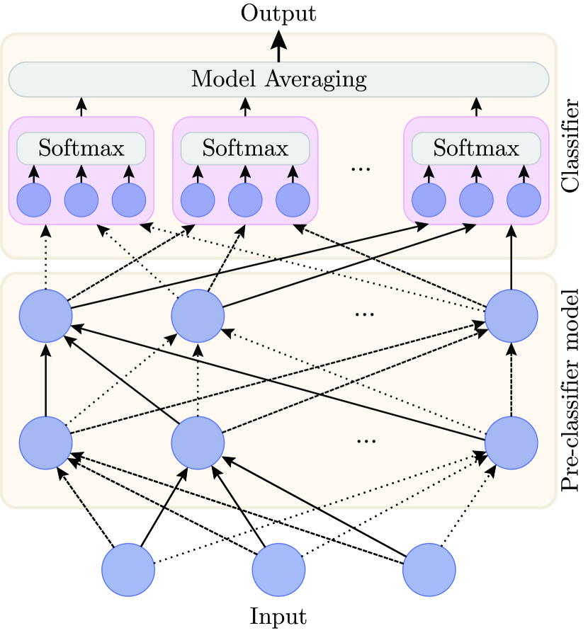
Principle.

Alrao starts with a standard optimization method such as SGD, and a range of possible learning rates $(\eta_{\min},\eta_{\max})$. Instead of using a single learning rate, we sample once and for all one learning rate for each feature, randomly sampled log-uniformly in $(\eta_{\min},\eta_{\max})$. Then these learning rates are used in the usual optimization update:

$$\theta_{l,i}\leftarrow\theta_{l,i}-\eta_{l,i}\cdot\nabla_{\theta_{l,i}}\ell(\Phi_{\theta}(x),y)$$ (1)

where $\theta_{l,i}$ is the set of parameters used to compute the feature $i$ of layer $l$ from the activations of layer $l-1$ (the incoming weights of feature $i$). Thus we build “slow-learning” and “fast-learning” features, in the hope to get enough features in the “Goldilocks zone”.

What constitutes a feature depends on the type of layers in the model. For example, in a fully connected layer, each component of a layer is considered as a feature: all incoming weights of the same unit share the same learning rate. On the other hand, in a convolutional layer we consider each convolution filter as constituting a feature: there is one learning rate per filter (or channel), thus keeping translation-invariance over the input image. In LSTMs, we apply the same learning rate to all components in each LSTM unit (thus in the implementation, the vector of learning rates is the same for input gates, for forget gates, etc.).

However, the update (1) cannot be used directly in the last layer. For instance, for regression there may be only one output feature. For classification, each feature in the final classification layer represents a single category, and so using different learning rates for these features would favor some categories during learning. Instead, on the output layer we chose to duplicate the layer using several learning rate values, and use a (Bayesian) model averaging method to obtain the overall network output (Fig. 1). Appendix B contains a proof (under convexity assumptions) that this mechanism works, given the initial layers.

We set a learning rate per feature, rather than per parameter. Otherwise, every feature would have some parameters with large learning rates, and we would expect even a few large incoming weights to be able to derail a feature. So having diverging parameters within a feature is hurtful, while having diverging features in a layer is not necessarily hurtful since the next layer can choose to disregard them.

Definitions and notation.

We now describe Alrao more precisely for deep learning models with softmax output, on classification tasks (the case of regression is similar).

Let $\mathcal{D}=\{(x_{1},y_{1}),...,(x_{N},y_{N})\}$, with $y_{i}\in\{1,...,K\}$, be a classification dataset. The goal is to predict the $y_{i}$ given the $x_{i}$, using a deep learning model $\Phi_{\theta}$. For each input $x$, $\Phi_{\theta}(x)$ is a probability distribution over $\{1,...,K\}$, and we want to minimize the categorical cross-entropy loss $\ell$ over the dataset: $\frac{1}{N}\sum_{i}\ell(\Phi_{\theta}(x_{i}),y_{i})$.

A deep learning model for classification $\Phi_{\theta}$ is made of two parts: a pre-classifier $\phi_{\theta^{\mathrm{pc}}}$ which computes some quantities fed to a final classifier layer $C_{\theta^{\mathrm{cl}}}$, namely, $\Phi_{\theta}(x)=C_{\theta^{\mathrm{cl}}}(\phi_{\theta^{\mathrm{pc}}}(x))$. The classifier layer $C_{\theta^{\mathrm{cl}}}$ with $K$ categories is defined by $C_{\theta^{\mathrm{cl}}}=\mathrm{softmax}\circ\left(W^{T}x+b\right)$ with $\theta^{\mathrm{cl}}=(W,b)$, and $\mathrm{softmax}(x_{1},...,x_{K})_{k}={e^{x_{k}}}/\left({\sum_{i}e^{x_{i}}}\right).$The pre-classifier is a computational graph composed of any number of layers, and each layer is made of multiple features.

We denote $\operatorname*{log-{\cal U}}(\cdot;\eta_{\min},\eta_{\max})$ the log-uniform probability distribution on an interval $(\eta_{\min},\eta_{\max})$: namely, if $\eta\sim\operatorname*{log-{\cal U}}(\cdot;\eta_{\min},\eta_{\max})$, then $\log\eta$ is uniformly distributed between $\log\eta_{\min}$ and $\log\eta_{\max}$. Its density function is

$$\operatorname*{log-{\cal U}}(\eta;\eta_{\min},\eta_{\max})=\frac{\mathbbm{1}_{\eta_{\min}\leq\eta\leq\eta_{\max}}}{\log(\eta_{\max})-\log(\eta_{\min})}\times\frac{1}{\eta}$$ (2)

Algorithm 1 Alrao for model $\Phi_{\theta}=C_{\theta^{\mathrm{cl}}}\circ\phi_{\theta^{\mathrm{pc}}}$ with $N_{\mathrm{cl}}$ classifiers and learning rates in $[\eta_{\min},\eta_{\max}]$

1:  $a_{j}\leftarrow 1/N_{\mathrm{cl}}$ for each $1\leq j\leq N_{\mathrm{cl}}$ // Initialize the $N_{\mathrm{cl}}$ model averaging weights $a_{j}$

2:  $\Phi^{\text{Alrao}}_{\theta}(x):=\sum_{j=1}^{N_{\mathrm{cl}}}a_{j}\,C_{\theta^{\mathrm{cl}}_{j}}(\phi_{\theta^{\mathrm{pc}}}(x))$ // Define the Alrao architecture

3:  for layers $l$, for all feature $i$ in layer $l$ do

4:     Sample $\eta_{l,i}\sim\operatorname*{log-{\cal U}}(.;\eta_{\min},\eta_{\max})$. // Sample a learning rate for each feature

5:  end for

6:  for classifiers $j$, $1\leq j\leq N_{\mathrm{cl}}$ do

7:     Define $\log\eta_{j}=\log\eta_{\min}+\frac{j-1}{N_{\mathrm{cl}}-1}\log\frac{\eta_{\max}}{\eta_{\min}}$. // Set a learning rate for each classifier $j$

8:  end for

9:  while stopping criterion is false do

10:     $z_{t}\leftarrow\phi_{\theta^{\mathrm{pc}}}(x_{t})$ // Store the pre-classifier output

11:     for layers $l$, for all feature $i$ in layer $l$ do

12:        $\theta_{l,i}\leftarrow\theta_{l,i}-\eta_{l,i}\cdot\nabla_{\theta_{l,i}}\ell(\Phi^{\text{Alrao}}_{\theta}(x_{t}),y_{t})$ // Update the pre-classifier weights

13:     end for

14:     for Classifier $j$ do

15:        $\theta^{\mathrm{cl}}_{j}\leftarrow\theta^{\mathrm{cl}}_{j}-\eta_{j}\cdot\nabla_{\theta^{\mathrm{cl}}_{j}}\,\ell(C_{\theta^{\mathrm{cl}}_{j}}(z_{t}),y_{t})$ // Update the classifiers’ weights

16:     end for

17:     $a\leftarrow\mathtt{ModelAveraging}(a,(C_{\theta^{\mathrm{cl}}_{i}}(z_{t}))_{i},y_{t})$ // Update the model averaging weights.

18:     $t\leftarrow t+1$ mod $N$

19:  end while

Alrao for the pre-classifier: A random learning rate for each feature.

In the pre-classifier, for each feature $i$ in each layer $l$, a learning rate $\eta_{l,i}$ is sampled from the probability distribution $\operatorname*{log-{\cal U}}(.;\eta_{\min},\eta_{\max})$, once and for all at the beginning of training. Then the incoming parameters of each feature in the preclassifier are updated in the usual way with this learning rate (Eq. 5).

Alrao for the classifier layer: Model averaging from classifiers with different learning rates.

In the classifier layer, we build multiple clones of the original classifier layer, set a different learning rate for each, and then use a model averaging method from among them. The averaged classifier and the overall Alrao model are:

$$C^{\text{Alrao}}_{\theta^{\mathrm{cl}}}(z)\mathrel{\mathop{:}}=\sum_{j=1}^{N_{\mathrm{cl}}}a_{j}\,C_{\theta^{\mathrm{cl}}_{j}}(z)$$ (3)

$$\Phi^{\text{Alrao}}_{\theta}(x)\mathrel{\mathop{:}}=C^{\text{Alrao}}_{\theta^{\mathrm{cl}}}(\phi_{\theta^{\mathrm{pc}}}(x))$$ (4)

where the $C_{\theta^{\mathrm{cl}}_{j}}$ are copies of the original classifier layer, with non-tied parameters, and $\theta^{\mathrm{cl}}\mathrel{\mathop{:}}=(\theta^{\mathrm{cl}}_{1},...,\theta^{\mathrm{cl}}_{N_{\mathrm{cl}}})$. The $a_{j}$ are the parameters of the model averaging, and are such that for all $j$, $0\leq a_{j}\leq 1$, and $\sum_{j}a_{j}=1$. These are not updated by gradient descent, but via a model averaging method from the literature (see below).

For each classifier $C_{\theta^{\mathrm{cl}}_{j}}$, we set a learning rate $\eta_{j}$ defined by $\log\eta_{j}=\log\eta_{\min}+\frac{j-1}{N_{\mathrm{cl}}-1}\log\left(\frac{\eta_{\max}}{\eta_{\min}}\right)$, so that the classifiers’ learning rates are log-uniformly spread on the interval $[\eta_{\min},\eta_{\max}]$.

Thus, the original model $\Phi_{\theta}(x)$ leads to the Alrao model $\Phi^{\text{Alrao}}_{\theta}(x)$. Only the classifier layer is modified, the pre-classifier architecture being unchanged.

Update rule.

Alg. 1 presents the full Alrao algorithm. The updates for the pre-classifier, classifier, and model averaging weights are as follows.

• The update rule for the pre-classifier is the usual SGD one, with per-feature learning rates. For each feature $i$ in each layer $l$, its incoming parameters are updated as:

  $$\theta_{l,i}\leftarrow\theta_{l,i}-\eta_{l,i}\cdot\nabla_{\theta_{l,i}}\ell(\Phi^{\text{Alrao}}_{\theta}(x),y)$$ (5)

• The parameters $\theta^{\mathrm{cl}}_{j}$ of each classifier clone $j$ on the classifier layer are updated as if this classifier alone was the only output of the model:

  $$\theta^{\mathrm{cl}}_{j}\leftarrow \;\theta^{\mathrm{cl}}_{j}-\eta_{j}\cdot\nabla_{\theta^{\mathrm{cl}}_{j}}\,\ell(C_{\theta^{\mathrm{cl}}_{j}}(\phi_{\theta^{\mathrm{pc}}}(x)),y)$$ (6)

  (still sharing the same pre-classifier $\phi_{\theta^{\mathrm{pc}}}$). This ensures classifiers with low weights $a_{j}$ still learn, and is consistent with model averaging philosophy. Algorithmically this requires differentiating the loss $N_{\mathrm{cl}}$ times with respect to the last layer (but no additional backpropagations through the preclassifier).

• To set the weights $a_{j}$, several model averaging techniques are available, such as Bayesian Model Averaging (Wasserman, 2000). We decided to use the Switch model averaging (Van Erven et al., 2012), a Bayesian method which is both simple, principled and very responsive to changes in performance of the various models. After each sample or mini-batch, the switch computes a modified posterior distribution $(a_{j})$ over the classifiers. This computation is directly taken from (Van Erven et al., 2012) and explained in Appendix A. The observed evolution of this posterior during training is commented upon in Appendix C.

Table 1: Performance of Alrao, of SGD with optimal learning rate from $\{10^{-5},10^{-4},10^{-3},10^{-2},10^{-1},1.,10.\}$, and of Adam with its default setting. Three convolutional models are reported for image classification on CIFAR10, three others for ImageNet, one recurrent model for character prediction (Penn Treebank), and two experiments on RL problems. The Alrao learning rates have been taken in wide a priori reasonable intervals, $[\eta_{\min};\eta_{\max}]=[10^{-5};10]$ for CNNs (CIFAR10 and ImageNet) and RL, and $[10^{-3};10^{2}]$ for RNNs (PTB). Each experiment is run 10 times (CIFAR10 and RL), 5 times (PTB) or 1 time (ImageNet); the confidence intervals report the standard deviation over these runs.

Model	SGD with optimal LR			Adam - Default		Alrao
	LR	Loss	Top1 (%)	Loss	Top1 (%)	Loss	Top1 (%)
CIFAR10
MobileNet	$1e$-1	$0.37\pm 0.01$	$90.2\pm 0.3$	$1.01\pm 0.95$	$78\pm 11$	$0.42\pm 0.02$	$88.1\pm 0.6$
MobileNet, width*3	-	-	-	$0.32\pm 0.02$	$90.8\pm 0.4$	$0.35\pm 0.01$	$89.0\pm 0.6$
GoogLeNet	$1e$-2	$0.45\pm 0.05$	$89.6\pm 1.0$	$0.47\pm 0.04$	$89.8\pm 0.4$	$0.47\pm 0.03$	$88.9\pm 0.8$
GoogLeNet, width*3	-	-	-	$0.41\pm 0.02$	$88.6\pm 0.6$	$0.37\pm 0.01$	$89.8\pm 0.8$
VGG19	$1e$-1	$0.42\pm 0.02$	$89.5\pm 0.2$	$0.43\pm 0.02$	$88.9\pm 0.4$	$0.45\pm 0.03$	$87.5\pm 0.4$
VGG19, width*3	-	-	-	$0.37\pm 0.01$	$89.5\pm 0.8$	$0.381\pm 0.004$	$88.4\pm 0.7$
ImageNet
AlexNet	$1e$-2	$2.15$	$53.2$	$6.91$	$0.10$	$2.56$	$43.2$
Densenet121	$1$	$1.35$	$69.7$	$1.39$	$67.9$	$1.41$	$67.3$
ResNet50	$1$	$1.49$	$67.4$	$1.39$	$67.1$	$1.42$	$67.5$
ResNet50, width*3	-	-	-	$1.99$	$60.8$	$1.33$	$70.9$
Penn Treebank
LSTM	$1$	$1.566\pm 0.003$	$66.1\pm 0.1$	$1.587\pm 0.005$	$65.6\pm 0.1$	$1.67\pm 0.01$	$64.1\pm 0.2$
Reinforcement Learning		Return		Return		Return
Pendulum	$1e-4$	$-372\pm 24$		$-414\pm 64$		$-371\pm 36$
LunarLander	$1e-1$	$188\pm 23$		$155\pm 23$		$186\pm 45$

Implementation.

We release along with this paper a Pytorch (Paszke et al., 2017) implementation of this method. It can be used on an existing model with little modification. A short tutorial is given in Appendix H. Features (sets of weights sharing the same learning rate) need to be specified for each layer type: for now this has been done for linear, convolutional, and LSTMs layers.

5 Experimental Setup

We tested Alrao on various convolutional networks for image classification (Imagenet and CIFAR10), on LSTMs for text prediction, and on Reinforcement Learning problems. The baselines are SGD with an optimal learning rate, and Adam with its default setting, arguably the current default method (Wilson et al., 2017).

Image classification on ImageNet and CIFAR10.

For image classification, we used the ImageNet (Deng et al., 2009) and CIFAR10 (Krizhevsky, 2009) datasets. The ImageNet dataset is made of 1,283,166 training and 60,000 testing data; we split the training set into a smaller training set and a validation set with 60,000 samples. We do the same on CIFAR10: the 50,000 training samples are split into 40,000 training samples and 10,000 validation samples.

For each architecture, training on the smaller training set was stopped when the validation loss had not improved for 20 epochs. The epoch with best validation loss was selected and the corresponding model tested on the test set. The inputs are normalized, and training used data augmentation: random cropping and random horizontal flipping (see Appendix D for details). For CIFAR10, each setting was run 10 times: the confidence intervals presented are the standard deviation over these runs. For ImageNet, because of high computation time, we performed only a single run per experiment.

We tested Alrao on several standard architectures for these tasks. On ImageNet, we tested Resnet50 (He et al., 2016), Densenet121 (Huang et al., 2017) and Alexnet (Krizhevsky, 2014), with the default Pytorch implementation. On CIFAR10, we tested GoogLeNet (Szegedy et al., 2015), VGG19 (Simonyan and Zisserman, 2014) and MobileNet (Howard et al., 2017) implemented by (Kianglu, 2018).

The Alrao learning rates were sampled log-uniformly from $\eta_{\min}=10^{-5}$ to $\eta_{\max}=10$. For the output layer we used 10 classifiers with switch model averaging (Appendix A); the learning rates of the output classifiers are deterministic and log-uniformly spread in $[\eta_{\min},\eta_{\max}]$.

In addition, each model was trained with SGD for every learning rate in the set $\{10^{-5},10^{-4},10^{-3},10^{-2},10^{-1},1.,10.\}$. The best SGD learning rate is selected on the validation set, then reported in Table 1. We also compare to Adam with its default hyperparameters ($\eta=10^{-3},\beta_{1}=0.9,\beta_{2}=0.999$).

Finally, since Alrao may waste units with unsuitable learning rates, we also tested architectures with increased width ($3$ times as many units) with Alrao and Adam on ImageNet and CIFAR10. On these larger models, systematic SGD learning rate grid search was not performed due to the time required.

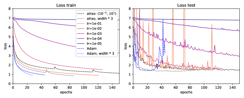
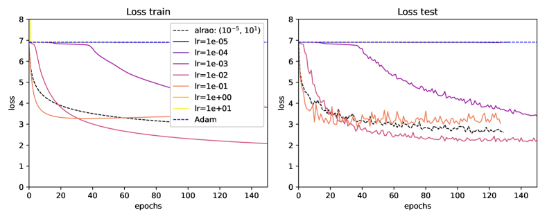
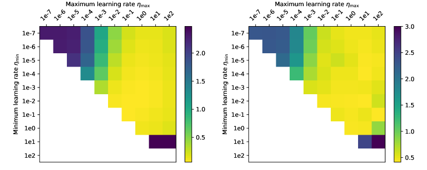
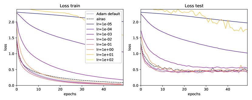
The results are presented in Table 1. Learning curves with various SGD learning rates, Adam and Alrao are presented in Fig. 2. Fig. 3 tests the influence of $\eta_{\min}$ and $\eta_{\max}$.

(a) Resnet50 on ImageNet.

(b) AlexNet on ImageNet

Figure 2: Learning curves for SGD with various learning rates, Alrao, and Adam with its default setting, with the Resnet50 architecture on ImageNet and the MobileNetV2 architecture on CIFAR10. Left: training loss; right: test loss. While Alrao uses learning rates from the entire range, its performance is comparable to the optimal learning rate.

Recurrent learning on Penn Treebank.

To test Alrao on a different kind of architecture, we used a recurrent neural network for text prediction on the Penn Treebank (Marcus et al., 1993) dataset. The experimental procedure is the same, with $(\eta_{\min},\eta_{\max})=(0.001,100)$ and $6$ output classifiers for Alrao. The results appear in Table 1, where the loss is given in bits per character and the accuracy is the proportion of correct character predictions.

The model was trained for character prediction rather than word prediction. This is technically easier for Alrao implementation: since Alrao uses copies of the output layer, memory issues arise for models with most parameters on the output layer. Word prediction (10,000 classes on PTB) requires more output parameters than character prediction; see Section 7 and Appendix F.

The model is a two-layer LSTM (Hochreiter and Schmidhuber, 1997) with an embedding size of 100 and 100 hidden features. A dropout layer with rate $0.2$ is included before the decoder. The training set is divided into 20 minibatchs. Gradients are computed via truncated backprop through time (Werbos, 1990) with truncation every 70 characters.

Reinforcement Learning.

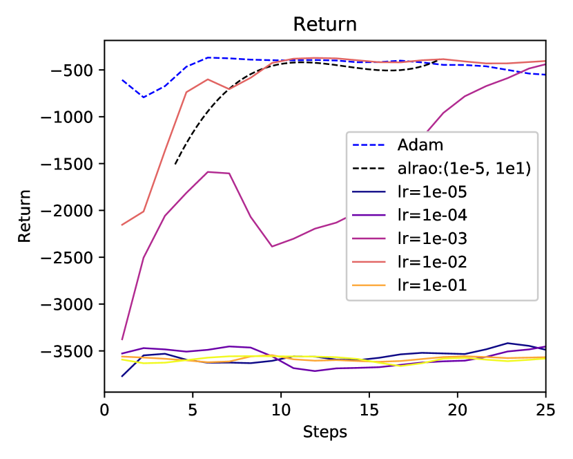
We tested Alrao on two standard Reinforcement Learning problems: the Pendulum and Lunar Lander environments from OpenAI Gym (Brockman et al., 2016). We use standard Deep Q-learning (Mnih et al., 2015). The $Q$-network is a standard MLP with 2 hidden layers. The experimental setting to compare Alrao, Adam and SGD is the same as above, with $\eta_{\min}=10^{-5}$ to $\eta_{\max}=10$. Alrao uses 10 output layers (which are not classifiers in that case but regressors). More details on the Q-learning implementation are given in Appendix D. For each environment, we selected the best epoch on evaluation runs, and then reported the return of the selected model on new runs in that environment.

6 Performance and Robustness of Alrao

Performance of Alrao compared to SGD with the optimal learning rate.

As expected, Alrao usually performs slightly worse than the best learning rate with SGD.

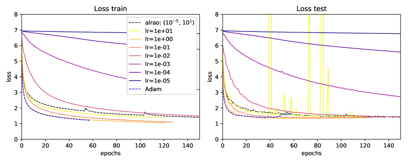
Still, even with wide intervals $(\eta_{\min},\eta_{\max})$, Alrao comes reasonably close to the best learning rate, across every setup. Notably, this occurs even though SGD achieves good performance only for a few learning rates within the interval $(\eta_{\min},\eta_{\max})$. With our setting for image classification and RL ($\eta_{\min}=10^{-5}$ and $\eta_{\max}=10$), among the $7$ learning rates used with SGD (${10^{-5},10^{-4},10^{-3},10^{-2},10^{-1},1,10}$), only 3 are able to learn with AlexNet (and only one is better than Alrao, see Fig. 2b), only 3 are able to learn with ResNet50 (and only two of them achieve performance similar to Alrao, see Fig. 2a), and only 2 are able to learn on the pendulum environment (and only one of them converges as fast as Alrao, Fig. 6 in Appendix D). More examples are in Appendix D. It is surprising that Alrao manages to learn even though most of the units in the network would have learning rates unsuited for SGD.

Robustness of Alrao compared to default Adam.

Overall, Alrao learns reliably in every setup. Performance is close to optimal SGD in all cases (Table 1) with a somewhat larger gap in one case (AlexNet on ImageNet). This observation is quite stable over the course of learning, with Alrao curves shadowing optimal SGD curves over time (Fig. 2).

Often, Adam with its default parameters almost matches optimal SGD, but this is not always the case. Over the 13 setups in Table 1, default Adam gives a significantly poor performance in three cases. One of those is a pure optimization issue: with AlexNet on ImageNet, optimization does not start (Fig. 2b) with default parameters. The other two cases are due to strong overfit despite good train performance: MobileNet on CIFAR (Fig. 5c in Appendix D) and ResNet with increased width on ImageNet (Fig. 2a).

In two further cases, Adam achieves good validation performance but overfits shortly thereafter: ResNet (Fig. 2a)and DenseNet (Fig. 5b in Appendix D), both on ImageNet). On the whole, this confirms a known risk of overfit with Adam (Wilson et al., 2017).

Overall, default Adam tends to give slightly better results than Alrao when it works, but does not learn reliably with its default hyperparameters. It can exhibit two kinds of lack of robustness: optimization failure, and overfit or non-robustness over the course of learning. On the other hand, every single run of Alrao reached reasonably close-to-optimal performance. Alrao also exhibits a steady performance over the course of learning (Fig. 2).

7 Limitations and Perspectives

Figure 3: Performance of Alrao with a GoogLeNet model on CIFAR10, depending on the interval $(\eta_{\min},\eta_{\max})$. Left: loss on the train set; right: on the test set. Each point with coordinates $(\eta_{\min},\eta_{\max})$ above the diagonal represents the loss after 30 epochs for Alrao with this interval. Points $(\eta,\eta)$ on the diagonal represent standard SGD with learning rate $\eta$ after 50 epochs. Standard SGD with $\eta=10^{2}$ is left blank to due numerical divergence (NaN). Alrao works as soon as $(\eta_{\min},\eta_{\max})$ contains at least one suitable learning rate.

Increased number of parameters for the classification layer.

Alrao modifies the output layer of the optimized model. The number of parameters for the classification layer is multiplied by the number of classifier copies used (the number of parameters in the pre-classifier is unchanged). On CIFAR10 (10 classes), the number of parameters increased by less than 5% for the models used. On ImageNet (1000 classes), it increases by 50–100% depending on the architecture. On Penn Treebank, the number of parameters increased by $15\%$ in our setup (working at the character level); working at word level it would have increased threefold (Appendix F). Still, models with a very large number of output classes usually rely on other parameterizations than a direct softmax, such as a hierarchical softmax (see references in (Jozefowicz et al., 2016)); Alrao can be used in conjunction with such methods.

This would clearly be a limitation of Alrao for models with most parameters in the classifier layer and without existing methods to streamline this layer. For such models, this could be mitigated by handling the copies of the classifiers on distinct computing units: in Alrao these copies work in parallel given the pre-classifier.

Adding two hyperparameters.

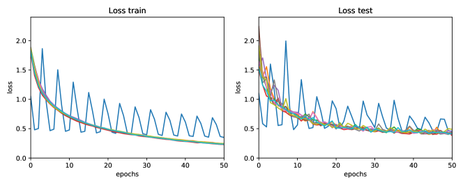
We claim to remove a hyperparameter, the learning rate, but replace it with two hyperparameters $\eta_{\min}$ and $\eta_{\max}$. Formally, this is true. But a systematic study of the impact of these two hyperparameters (Fig. 3) shows that the sensitivity to $\eta_{\min}$ and $\eta_{\max}$ is much lower than the original sensitivity to the learning rate. In our experiments, convergence happens as soon as $(\eta_{\min};\eta_{\max})$ contains a reasonable learning rate (Fig. 3).

A wide range of values of $(\eta_{\min};\eta_{\max})$ will contain one good learning rate and achieve close-to-optimal performance (Fig. 3). Typically, we recommend to just use an interval containing all the learning rates that would have been tested in a grid search, e.g., $10^{-5}$ to $10$.

So, even if the choice of $\eta_{\min}$ and $\eta_{\max}$ is important, the results are much more stable to varying these two hyperparameters than to the original learning rate. For instance, standard SGD fails due to numerical issues for $\eta=100$ while Alrao with $\eta_{\max}=100$ works with any $\eta_{\min}\leq 1$ (Fig. 3), and is thus stable to relatively large learning rates. We would still expect numerical issues with very large $\eta_{\max}$, but this has not been observed in our experiments.

Increasing network size.

With Alrao, neurons with unsuitable learning rates will not learn: those with a too large learning rate might learn nothing, while those with too small learning rates will learn too slowly to be used. Thus, Alrao may reduce the effective size of the network to only a fraction of the actual architecture size, depending on $(\eta_{\min},\eta_{\max})$. Our first intuition was that increasing the width of the network was going to be necessary with Alrao, to avoid wasting too many units.

Tests of Alrao with increased width are reported in Table 1 and Fig. 2a.Incidentally, these tests show that width was a limiting factor of the models used for both Alrao and SGD. Still, to our surprise, Alrao worked well even without width augmentation.

Other optimizers, other hyperparameters, learning rate schedulers…

Using a learning rate schedule instead of a fixed learning rate is often effective (Bengio, 2012). We did not use learning rate schedulers here; this may partially explain why the results in Table 1 are worse than the state-of-the-art. Nothing prevents using such a scheduler within Alrao, e.g., by dividing all Alrao learning rates by a time-dependent constant; we did not experiment with this yet. One might have hoped that Alrao would match good stepsize schedules thanks to the diversity of learning rates, but our results do not currently support this.

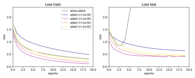
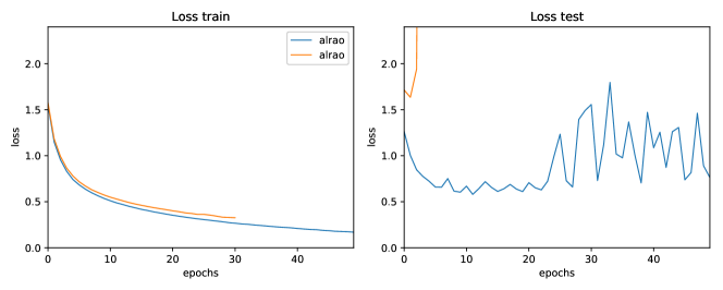
The Alrao idea can also be used with other optimizers than SGD, such as Adam. We tested combining Alrao and Adam, and found the combination less reliable than standard Alrao (Appendix E, Fig. 7). This occurs mostly for test performance, while training curves mostly look good (Fig. 7). The stark train/test discrepancy suggests that Alrao combined with Adam may perform well as a pure optimization method but exacerbates the underlying risk of overfit of Adam (Wilson et al., 2017; Keskar and Socher, 2017).

The Alrao idea could be used on other hyperparameters as well, such as momentum. However, if more hyperparameters are initialized randomly for each feature, the fraction of features having all their hyperparameters in the “Goldilocks zone” will quickly decrease.

8 Conclusion

Applying stochastic gradient descent with multiple learning rates for different features is surprisingly resilient in our experiments, and provides performance close enough to SGD with an optimal learning rate, as soon as the range of random learning rates contains a suitable one. The same resilience is not observed with default Adam. Alrao could save time when testing deep learning models, opening the door to more out-of-the-box uses of deep learning.

Appendix A Model Averaging with the Switch

As explained is Section 4, we use a model averaging method on the classifiers of the output layer. We could have used the Bayesian Model Averaging method [Wasserman, 2000]. But one of its main weaknesses is the catch-up phenomenon [Van Erven et al., 2012]: plain Bayesian posteriors are slow to react when the relative performance of models changes over time. Typically, for instance, some larger-dimensional models need more training data to reach good performance: at the time they become better than lower-dimensional models for predicting current data, their Bayesian posterior is so bad that they are not used right away (their posterior needs to “catch up” on their bad initial performance). This leads to very conservative model averaging methods.

The solution from [Van Erven et al., 2012] against the catch-up phenomenon is to switch between models. It is based on previous methods for prediction with expert advice (see for instance [Herbster and Warmuth, 1998, Volf and Willems, 1998] and the references in [Koolen and De Rooij, 2008, Van Erven et al., 2012]), and is well rooted in information theory. The switch method maintains a Bayesian posterior distribution, not over the set of models, but over the set of switching strategies between models. Intuitively, the model selected can be adapted online to the number of samples seen.

We now give a quick overview of the switch method from [Van Erven et al., 2012]: this is how the model averaging weights $a_{j}$ are chosen in Alrao.

Assume that we have a set of prediction strategies $\mathcal{M}=\{p^{j},j\in\mathcal{I}\}$. We define the set of switch sequences, $\mathbb{S}=\{((t_{1},j_{1}),...,(t_{L},j_{L})),1=t_{1}<t_{2}<...<t_{L}\;,\;j\in\mathcal{I}\}$. Let $s=((t_{1},j_{1}),...,(t_{L},j_{L}))$ be a switch sequence. The associated prediction strategy $p_{s}(y_{1:n}|x_{1:n})$ uses model $p^{j_{i}}$ on the time interval $[t_{i};t_{i+1})$, namely

$$p_{s}(y_{1:i+1}|x_{1:i+1},y_{1:i})=p^{K_{i}}(y_{i+1}|x_{1:i+1},y_{1:i})$$ (7)

where $K_{i}$ is such that $K_{i}=j_{l}$ for $t_{l}\leq i<t_{l+1}$. We fix a prior distribution $\pi$ over switching sequences. In this work, ${\cal I}=\{1,...,N_{C}\}$ the prior is, for a switch sequence $s=((t_{1},j_{1}),...,(t_{L},j_{L}))$:

$$\pi(s)=\pi_{L}(L)\pi_{K}(j_{1})\prod_{i=2}^{L}\pi_{T}(t_{i}|t_{i}>t_{i-1})\pi_{K}(j_{i})$$ (8)

with $\pi_{L}(L)=\frac{\theta^{L}}{1-\theta}$ a geometric distribution over the switch sequences lengths, $\pi_{K}(j)=\frac{1}{N_{C}}$ the uniform distribution over the models (here the classifiers) and $\pi_{T}(t)=\frac{1}{t(t+1)}$.

This defines a Bayesian mixture distribution:

$$p_{sw}(y_{1:T}|x_{1:T})=\sum_{s\in\mathbb{S}}\pi(s)p_{s}(y_{1:T}|x_{1:T})$$ (9)

Then, the model averaging weight $a_{j}$ for the classifier $j$ after seeing $T$ samples is the posterior of the switch distribution: $\pi(K_{T+1}=j|y_{1:T},x_{1:T})$.

$$a_{j} =p_{sw}(K_{T+1}=j|y_{1:T},x_{1:T})$$ (10)

$$=\frac{p_{sw}(y_{1:T},K_{T+1}=j|x_{1:T})}{p_{sw}(y_{1:T}|x_{1:T})}$$ (11)

These weights can be computed online exactly in a quick and simple way [Van Erven et al., 2012], thanks to dynamic programming methods from hidden Markov models.

The implementation of the switch used in Alrao exactly follows the pseudo-code from [Van Erven et al., 2008], with hyperparameter $\theta=0.999$ (allowing for many switches a priori). It can be found in the accompanying online code.

Appendix B Convergence result in a simple case

We prove a convergence result on Alrao in a simplified case: we assume that the loss is convex, that the pre-classifier is fixed, that we work with full batch gradients rather than stochastic gradient descent, and that the Alrao model averaging method is standard Bayesian model averaging. The convexity and fixed classifier assumptions cover, for instance, standard logistic regression: in that case the Alrao output layer contains copies of a logistic classifier with various learning rates, and the Alrao pre-classifier is the identity (or any fixed linear pre-classifier).

For each Alrao classifier $j$, for simplicity we denote its parameters by $\theta_{j}$ instead of $\theta_{j}^{\text{cl}}$ (there is no more ambiguity since the pre-classifier is fixed).

The loss of some classifier $C$ on a dataset with features $(x_{i})$ and labels $(y_{i})$ is $L(C)\mathrel{\mathop{:}}=\frac{1}{N}\sum_{i}\ell(C(x_{i}),y_{i})$, where for each input $x_{i}$, $(C(x_{i})_{y})_{y\in{\cal Y}}$ is a probability distribution over the possible labels $y\in{\cal Y}$, and we use the log-loss $\ell(C(x_{i}),y_{i})\mathrel{\mathop{:}}=-\log C(x_{i})_{y_{i}}$.

For a classifier $C_{\theta}$ with parameter $\theta$, let us abbreviate $L(\theta)\mathrel{\mathop{:}}=L(C_{\theta})$. We assume that $L(\theta)$ is a non-negative convex function, with $\nabla^{2}L(\theta)\preceq\lambda I$ for all $\theta$. Let $L^{*}$ be its global infimum; we assume $L^{*}$ is a minimum, reached at some point $\theta^{*}$, namely $L(\theta^{*})=L^{*}$. Moreover we assume that $L$ is locally strongly convex at its minimum $\theta^{*}$: $\nabla^{2}L(\theta^{*})\succ 0$.

The Alrao architecture for such a classifier $C_{\theta}$ uses $N_{\text{cl}}$ copies of the same classifier, with different parameter values:

$$\Phi^{\operatorname*{Alrao}}_{\theta_{\operatorname*{Alrao}}}(x)=\sum_{j=1}^{N_{\text{cl}}}a_{j}C_{\theta_{j}}$$ (12)

where $\theta_{\operatorname*{Alrao}}\mathrel{\mathop{:}}=(\theta_{1},...,\theta_{N_{\text{cl}}})$, and where the $(a_{j})_{j}$ are the weights given by the model averaging method. We abbreviate $L(\theta_{\operatorname*{Alrao}})\mathrel{\mathop{:}}=L(\Phi^{\operatorname*{Alrao}}_{\theta_{\operatorname*{Alrao}}})$.

The Alrao classification layer uses a set of learning rates $(\eta_{j})_{j\in J}$, and starting points $(\theta_{j}^{(0)})_{j\in J}$. Using full-batch (non stochastic) Alrao updates we have

$$\theta_{j}^{(t+1)} =\theta_{j}^{(t)}-\eta_{j}\nabla L(\theta_{j}^{(t)})$$ (13)

$$a^{(t+1)} =\mathtt{ModelAveraging}(a^{(t)},(C_{\theta_{i}}(x_{1:N}))_{i},y_{1:N})$$ (14)

We assume that the model averaging method is Bayesian Model Averaging.

We have assumed that the Hessian of the loss of the model satisfies $\nabla^{2}L(\theta)\preceq\lambda I$. Under this condition, the standard theory of gradient descent for convex functions requires that the learning rate be less than $1/\lambda$, otherwise the gradient descent might diverge. Therefore, for Alrao we assume that at least one of the learning rates considered by Alrao is below this threshold.

Theorem 1.

Assume that at least one of the Alrao learning rates $\eta_{j}$ satisfies $\eta_{j}<1/\lambda$, with $\lambda$ as above. Then, under the assumptions above, the Alrao loss is at most the optimal loss when $t\to\infty$:

$$\limsup_{t}L(\theta_{\operatorname*{Alrao}}^{(t)})\leq L^{*}$$ (15)

Proof.

Let us analyze the dynamics of the different models in the model averaging method. Let us split the set of Alrao classifiers in two categories according to whether their sum of errors is finite or infinite, namely,

$$A \mathrel{\mathop{:}}=\left\{j\in J\text{ such that }\sum_{t\geq 0}\left(L(\theta_{j}^{(t)})-L^{*}\right)<\infty\right\},$$ (16)

$$B \mathrel{\mathop{:}}=\left\{j\in J\text{ such that }\sum_{t\geq 0}\left(L(\theta_{j}^{(t)})-L^{*}\right)=\infty\right\}$$ (17)

and in particular, for any $j\in A$, $\lim_{t}L(\theta_{j}^{(t)})=L^{*}$.

The proof is organized as follows: We first show that $A$ is not empty. Then, we show that $\lim_{t\rightarrow\infty}a_{j}^{(t)}=0$ for all $j\in B$: these models are eliminated by the model averaging method. Then we will be able to conclude.

First, we show that $A$ is not empty: namely, that there is least one $j$ such that $\sum_{t\geq 0}(L(\theta_{j}^{(t)})-L^{*})<\infty$. We know that there is $j$ such that $\eta_{j}<\frac{2}{\lambda}$. Hence, the standard theory of gradient descent for convex functions shows that this particular classifier converges (e.g., [Tibshirani and Marchetti-Bowick, 2013]), namely, the loss $(L(\theta_{j}^{(t)}))_{t}$ converges to $L^{*}$. Moreover, since $L$ is localy stricly convex around $\theta^{*}$, this implies that $\lim_{t}\theta_{j}^{(t)}=\theta^{*}$.

We now show that the sum of errors for this specific $j$ converges. We assumed that $L(\theta)$ is locally strongly convex in $\theta^{*}$. Let $\mu>0$ such that $\nabla^{2}L(\theta^{*})\succeq\mu I$. Since $L$ is $C^{2}$, there is $\varepsilon^{\prime}$ such that for any $\theta$ such that $\|\theta-\theta^{*}\|\leq\varepsilon^{\prime}$, then $\nabla^{2}L(\theta)\succeq\frac{\mu}{2}I$. Let $\tau\in\mathbb{N}$ such that $\|\theta_{j}^{(\tau)}-\theta^{*}\|<\varepsilon^{\prime}$. Then, from the theory of gradient descent for strongly convex functions [Tibshirani and Marchetti-Bowick, 2013], we know there is some $\gamma<1$ such that for $t>\tau$, $L(\theta_{j}^{(t)})-L^{*}\leq C\|\theta_{j}^{(\tau)}-\theta^{*}\|\gamma^{t}$. We have:

$$\sum_{s=1}^{t} \left(L(\theta_{j}^{(s)})-L^{*}\right)=$$ (18)

$$=\sum_{s=1}^{\tau}\left(L(\theta_{j}^{(s)})-L^{*}\right)+\sum_{s=\tau}^{t}\left(L(\theta_{j}^{(s)})-L^{*}\right)$$ (19)

$$\leq\sum_{s=1}^{\tau}\left(L(\theta_{j}^{(s)})-L^{*}\right)+C\|\theta_{j}^{(\tau)}-\theta^{*}\|\gamma^{\tau}\frac{1}{1-\gamma}$$ (20)

Thus $\sum_{t\geq 0}\left(L(\theta_{j}^{(t)})-L^{*}\right)<\infty$. Therefore, $A$ is not empty.

We now show that the weights $a_{j}^{(t)}$ tend to $0$ for any $j\in B$, namely, $\lim_{t\rightarrow\infty}a_{j}^{(t)}=0$. Let $j\in B$ and take some $i\in A$. In Bayesian model averaging, the weights are

$$a_{j}^{(t)}{} =\frac{\prod_{s=1}^{t}p_{\theta_{j}^{(s)}}(y_{1:N}|x_{1:N})}{\sum_{k}\prod_{s=1}^{t}p_{\theta_{k}^{(s)}}(y_{1:N}|x_{1:N})}$$ (21)

$$\leq\prod_{s=1}^{t}\frac{p_{\theta_{j}^{(s)}}(y_{1:N}|x_{1:N})}{p_{\theta_{i}^{(s)}}(y_{1:N}|x_{1:N})}$$ (22)

$$=\prod_{s=1}^{t}\frac{\exp(-NL(\theta_{j}^{(s)}))}{\exp(-NL(\theta_{i}^{(s)}))}$$ (23)

$$\begin{split}{}&=\exp\Big{(}-N\sum_{s=1}^{t}\left(L(\theta_{j}^{(s)})-L^{*}\right)+\\ &N\sum_{s=1}^{t}\left(L(\theta_{i}^{(s)})-L^{*}\right)\Big{)}\end{split}$$ (24)

Since $i\in A$ and $j\in B$, by definition of $A$ and $B$ this tends to $0$. Therefore, $\lim_{t}a_{j}^{(t)}=0$ for all $j\in B$.

We now prove the statement of the theorem. We have:

$$\begin{split}L(\theta_{\operatorname*{Alrao}}^{(t)})={}&\frac{1}{N}\sum_{i}-\log\Big{(}\sum_{j\in A}a_{j}e^{-\ell(C_{\theta_{j}^{(t)}}(x_{i}),y_{i})}+\\ &\sum_{j\in B}a_{j}e^{-\ell(C_{\theta_{j}^{(t)}}(x_{i}),y_{i})}\Big{)}\end{split}$$ (25)

$$\leq\frac{1}{N}\sum_{i}-\log\left(\sum_{j\in A}a_{j}e^{-\ell(C_{\theta_{j}^{(t)}}(x_{i}),y_{i})}\right)$$ (26)

For all $i\in A$, set $\tilde{a}_{i}^{(t)}\mathrel{\mathop{:}}=\frac{a_{i}^{(t)}}{\sum_{j\in A}a_{j}^{(t)}}=\frac{a_{i}^{(t)}}{1-\sum_{j\in B}a_{j}^{(t)}}$. Then

$$\begin{split}L(\theta_{\operatorname*{Alrao}}^{(t)})\leq{}&-\log\left(1-\sum_{j\in B}a_{j}^{(t)}\right)\\ &+\frac{1}{N}\sum_{i}-\log\left(\sum_{j\in A}\tilde{a}_{j}e^{-\ell(C_{\theta_{j}^{(t)}}(x_{i}),y_{i})}\right)\end{split}$$ (27)

$$\leq\frac{1}{N}\sum_{i}\sum_{j\in A}\tilde{a}_{j}\ell(C_{\theta_{j}^{(t)}}(x_{i}),y_{i})+o(1)$$ (28)

$$=\sum_{j\in A}\tilde{a}_{j}L(\theta_{j}^{(t)})+o(1)$$ (29)

$$=L^{*}+o(1)$$ (30)

thanks to Jensen’s inequality for $-\log$, then because $\lim_{t}a_{j}^{(t)}=0$ for $j\in B$, and finally because $\lim_{t}L(\theta_{j}^{(t)})=L^{*}$ for $j\in A$. Taking the $\limsup$, we have:

$$\limsup_{t}L(\theta_{\operatorname*{Alrao}}^{(t)})\leq L^{*}$$ (31)

which ends the proof.∎

Appendix C Evolution of the Posterior

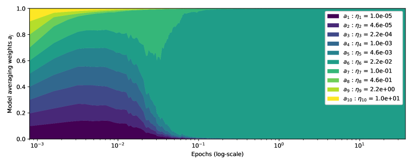
The evolution of the model averaging weights can be observed during training. In Figure 4, we can see their evolution during the training of the GoogLeNet model with Alrao on CIFAR10, 10 classifiers, with $\eta_{\min}=10^{-5}$ and $\eta_{\max}=10^{1}$.

We can make several observations. First, after only a few gradient descent steps, the model averaging weights corresponding to the three classifiers with the largest learning rates go to zero. This means that their parameters are moving too fast, and their loss is getting very large.

Next, for a short time, a classifier with a moderately large learning rate gets the largest posterior weight, presumably because it is the first to learn a useful model.

Finally, after the model has seen approximately 4,000 samples, a classifier with a slightly smaller learning rate is assigned a posterior weight $a_{j}$ close to 1, while all the others go to 0. This means that after a number of gradient steps, the model averaging method acts like a model selection method.

Figure 4: Model averaging weights during training. During the training of the GoogLeNet model with Alrao on CIFAR10, 10 classifiers, with $\eta_{\min}=10^{-5}$ and $\eta_{\max}=10^{1}$, we represent the evolution of the model averaging weights $a_{j}$, depending on the corresponding classifier’s learning rate.

Appendix D Additional Experimental Details and Results

In the case of CIFAR-10 and ImageNet, we normalize each input channel $x_{i}$ ($1\leq i\leq 3$), using its mean and its standard deviation over the training set. Let $\mu_{i}$ and $\sigma_{i}$ be respectively the mean and the standard deviation of the $i$-th channel. Then each input $(x_{1},x_{2},x_{3})$ is transformed into $(\frac{x_{1}-\mu_{1}}{\sigma_{1}},\frac{x_{2}-\mu_{2}}{\sigma_{2}},\frac{x_{3}-\mu_{3}}{\sigma_{3}})$. This operation is done over all the data (training, validation and test).

Moreover, we use data augmentation: every time an image of the training set is sent as input of the NN, this image is randomly cropped and and randomly flipped horizontally. Cropping consists in filling with black a band at the top, bottom, left and right of the image. The size of this band is randomly chosen between 0 and 4 in our experiments.

On CIFAR10 and PTB, the batch size was 32 for every architecture. On ImageNet, the batch-size is 256 for Alexnet and ResNet50, and 128 for Densenet121.

On the Reinforcement Learning environments, we used vanilla Q-learning [Mnih et al., 2015] with a soft target update as in [Lillicrap et al., 2015] $\tau=0.9$, and a memory buffer of size 1,000,000. The architecture for the Q network is a MLP with $2$ hidden layers. The learning curves are in Fig. 6. For the optimisation, the switch was used with 10 output layers. An output layer is a linear layer. Since the switch is a probability model averaging method, we consider each output layer as a probabilistic model, defined as a Normal distribution with variance 1 and mean the predicted value by the output layer. The loss for the Alrao model is the negative log-likelihood of the model mixture.

(a) GoogLeNet on CIFAR10 (Average on three runs)

(b) Densenet121 trained on ImageNet

(c) MobileNetV2 on Cifar10 (average over 3 runs)

Figure 5: Additional learning curves for SGD with various learning rates, Alrao, and Adam with its default setting, with the Densenet121 and Alexnet architectures on ImageNet and the GoogLeNet architecture on CIFAR10. Left: training loss; right: test loss.

Figure 6: Learning curves for the Reinforcement Learning environment in the pendulum environment in Q-learning, for SGD with various learning rates, Alrao, and Adam with its default setting

Appendix E Alrao with Adam

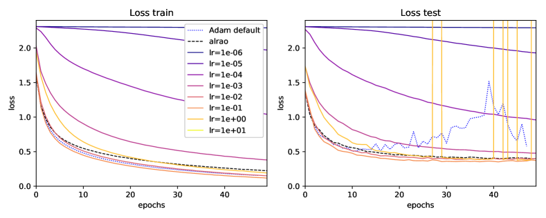
In Figure 7, we report our experiments with Alrao-Adam on CIFAR10. As explained in Section 7, Alrao is much less reliable with Adam than with SGD.

This is especially true for the test performance, which can even diverge while training performance remains either good or acceptable (Fig. 7). Thus Alrao-Adam seems to send the model into atypical regions of the search space.

We have no definitive explanation for this at present. It might be that changing Adam’s learning rate requires changing its momentum parameters accordingly. It might be that Alrao does not work on Adam because Adam is more sensitive to its hyperparameters.

(a) Alrao-Adam with GoogLeNet on CIFAR10: Alrao-Adam compared with standard Adam with various learning rates. Alrao uses 10 classifiers and learning rates in the interval $(10^{-6},1)$. Each plot is averaged on 10 experiments. We observe that optimization with Alrao-Adam is efficient, since train loss is comparable to the usual Adam methods. But the model starkly overfits, as the test loss diverges.

(b) Alrao-Adam with MobileNet on CIFAR10: Alrao-Adam with two different learning rate intervals, $(10^{-6},10^{-2})$ for the first one, $(10^{-6},10^{-1})$ for the second one, with 10 classifiers each. The first one is with $\eta_{\min}=10^{-6}$. Each plot is averaged on 10 experiments. Exactly as with GoogLeNet model, optimization itself is efficient (for both intervals). For the interval with the smallest $\eta_{\max}$, the test loss does not converge and is very unstable. For the interval with the largest $\eta_{\max}$, the test loss diverges.

(c) Alrao-Adam with VGG19 on CIFAR10: Alrao-Adam on the interval $(10^{-6},1)$, with 10 classifiers. The 10 plots are 10 runs of the same experiments. While 9 of them do converge and generalize, the last one exhibits wide oscillations, both in train and test.

Figure 7: Alrao-Adam: Experiments with the VGG19, GoogLeNet and MobileNet networks on CIFAR10.

Appendix F Number of Parameters

As explained in Section 7, Alrao increases the number of parameters of a model, due to output layer copies. The additional number of parameters is approximately equal to $(N_{\mathrm{cl}}-1)\times K\times d$ where $N_{\mathrm{cl}}$ is the number of classifier copies used in Alrao, $d$ is the dimension of the output of the pre-classifier, and $K$ is the number of classes in the classification task (assuming a standard softmax output; classification with many classes often uses other kinds of output parameterization instead).

Table 2: Comparison between the number of parameters in models used without and with Alrao. LSTM (C) is a simple LSTM cell used for character prediction while LSTM (W) is the same cell used for word prediction.

Model	Number of parameters
	Without Alrao	With Alrao
GoogLeNet	6.166M	6.258M
VGG	20.041M	20.087M
MobileNet	2.297M	2.412M
LSTM (C)	0.172M	0.197M
LSTM (W)	2.171M	7.221M

The number of parameters for the models used, with and without Alrao, are in Table 2. We used 10 classifiers in Alrao for convolutional neural networks, and 6 classifiers for LSTMs. Using Alrao for classification tasks with many classes, such as word prediction (10,000 classes on PTB), increases the number of parameters noticeably.

For those model with significant parameter increase, the various classifier copies may be done on parallel GPUs.

Appendix G Frozen Features Do Not Hurt Training

Figure 8: Loss of a model where only a random fraction $p$ of the features are trained, and the others left at their initial value, as a function of $p$. The architecture is GoogLeNet, trained on CIFAR10.

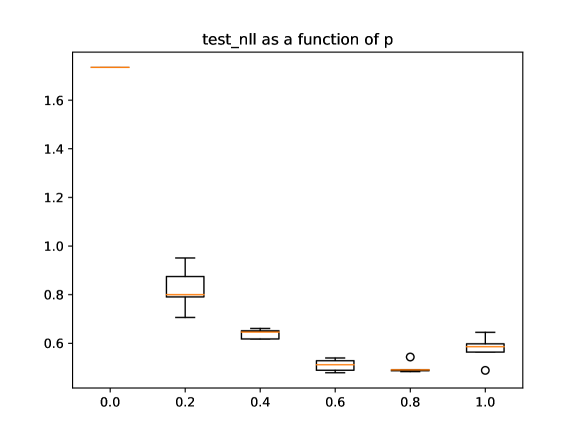
As explained in the introduction, several works support the idea that not all units are useful when learning a deep learning model. Additional results supporting this hypothesis are presented in Figure 8. We trained a GoogLeNet architecture on CIFAR10 with standard SGD with learning rate $\eta_{0}$, but learned only a random fraction $p$ of the features (chosen at startup), and kept the others at their initial value. This is equivalent to sampling each learning rate $\eta$ from the probability distribution $P(\eta=\eta_{0})=p$ and $P(\eta=0)=1-p$.

We observe that even with a fraction of the weights not being learned, the model’s performance is close to its performance when fully trained.

When training a model with Alrao, many features might not learn at all, due to too small learning rates. But Alrao is still able to reach good results. This could be explained by the resilience of neural networks to partial training.

Appendix H Tutorial

In this section, we briefly show how Alrao can be used in practice on an already implemented method in Pytorch. The full code will be available once the anonymity constraint is lifted.

The first step is to build the preclassifier. Here, we use the VGG19 architecture. The model is built without a classifier. Nothing else is required for Alrao at this step.

⬇

class VGG(nn.Module):

def __init__(self, cfg):

super(VGG, self).__init__()

self.features = self._make_layers(cfg)

# The dimension of the preclassier’s output need to be specified.

self.linearinputdim = 512

def forward(self, x):

out = self.features(x)

out = out.view(out.size(0), -1)

# The model do not contain a classifier layer.

return out

def _make_layers(self, cfg):

layers = []

in_channels = 3

for x in cfg:

if x == ’M’:

layers += [nn.MaxPool2d(kernel_size=2, stride=2)]

else:

layers += [nn.Conv2d(in_channels, x, kernel_size=3, padding=1),

nn.BatchNorm2d(x),

nn.ReLU(inplace=True)]

in_channels = x

layers += [nn.AvgPool2d(kernel_size=1, stride=1)]

return nn.Sequential(*layers)

preclassifier = VGG([64, 64, ’M’, 128, 128, ’M’, 256, 256, 256, 256, ’M’, \

512, 512, 512, 512, ’M’, 512, 512, 512, 512, ’M’])

Then, we can build the Alrao-model with this preclassifier, sample the learning rates for the model, and define the Alrao optimizer

⬇

# We define the interval in which the learning rates are sampled

minlr = 10 ** (-5)

maxlr = 10 ** 1

# nb_classifiers is the number of classifiers averaged by Alrao.

nb_classifiers = 10

nb_categories = 10

net = AlraoModel(preclassifier, nb_categories, preclassifier.linearinputdim, nb_classifiers)

# We spread the classifiers learning rates log-uniformly on the interval.

classifiers_lr = [np.exp(np.log(minlr) + \

k /(nb_classifiers-1) * (np.log(maxlr) - np.log(minlr)) \

) for k in range(nb_classifiers)]

# We define the sampler for the preclassifier’s features.

lr_sampler = lr_sampler_generic(minlr, maxlr)

lr_preclassifier = generator_randomlr_neurons(net.preclassifier, lr_sampler)

# We define the optimizer

optimizer = SGDAlrao(net.parameters_preclassifier(),

lr_preclassifier,

net.classifiers_parameters_list(),

classifiers_lr)

Finally, we can train the model. The only differences here with the usual training procedure is that each classifier needs to be updated as if it was alone, and that we need to update the model averaging weights, here the switch weights.

⬇

def train(epoch):

for batch_idx, (inputs, targets) in enumerate(trainloader):

# We update the model averaging weights in the optimizer

optimizer.update_posterior(net.posterior())

optimizer.zero_grad()

# Forward pass of the Alrao model

outputs = net(inputs)

loss = nn.NLLLoss(outputs, targets)

# We compute the gradient of all the model’s weights

loss.backward()

# We reset all the classifiers gradients, and re-compute them with

# as if their were the only output of the network.

optimizer.classifiers_zero_grad()

newx = net.last_x.detach()

for classifier in net.classifiers():

loss_classifier = criterion(classifier(newx), targets)

loss_classifier.backward()

# Then, we can run an update step of the gradient descent.

optimizer.step()

# Finally, we update the model averaging weights

net.update_switch(targets, catch_up=False)

References

- Amari [1998] Shun-ichi Amari. Natural gradient works efficiently in learning. Neural Comput., 10:251–276, February 1998. ISSN 0899-7667. doi: 10.1162/089976698300017746.
- Baker et al. [2016] Bowen Baker, Otkrist Gupta, Nikhil Naik, and Ramesh Raskar. Designing neural network architectures using reinforcement learning. arXiv preprint arXiv:1611.02167, 2016.
- Bengio [2012] Yoshua Bengio. Practical recommendations for gradient-based training of deep architectures. In Neural networks: Tricks of the trade, pages 437–478. Springer, 2012.
- Bergstra et al. [2013] James Bergstra, Daniel Yamins, and David Daniel Cox. Making a science of model search: Hyperparameter optimization in hundreds of dimensions for vision architectures. 2013.
- Brockman et al. [2016] Greg Brockman, Vicki Cheung, Ludwig Pettersson, Jonas Schneider, John Schulman, Jie Tang, and Wojciech Zaremba. Openai gym, 2016.
- Deng et al. [2009] J. Deng, W. Dong, R. Socher, L.-J. Li, K. Li, and L. Fei-Fei. ImageNet: A Large-Scale Hierarchical Image Database. In CVPR09, 2009.
- Denkowski and Neubig [2017] Michael Denkowski and Graham Neubig. Stronger baselines for trustable results in neural machine translation. arXiv preprint arXiv:1706.09733, 2017.
- Duchi et al. [2011] John Duchi, Elad Hazan, and Yoram Singer. Adaptive subgradient methods for online learning and stochastic optimization. The Journal of Machine Learning Research, 12:2121–2159, 2011.
- Frankle and Carbin [2018] Jonathan Frankle and Michael Carbin. The Lottery Ticket Hypothesis: Finding Small, Trainable Neural Networks. arXiv preprint arXiv:1704.04861, mar 2018.
- Guyon et al. [2016] Isabelle Guyon, Imad Chaabane, Hugo Jair Escalante, Sergio Escalera, Damir Jajetic, James Robert Lloyd, Núria Macià, Bisakha Ray, Lukasz Romaszko, Michèle Sebag, et al. A brief review of the ChaLearn AutoML challenge: any-time any-dataset learning without human intervention. In Workshop on Automatic Machine Learning, pages 21–30, 2016.
- Han et al. [2015a] Song Han, Huizi Mao, and William J. Dally. Deep Compression: Compressing Deep Neural Networks with Pruning, Trained Quantization and Huffman Coding. arXiv preprint arXiv:1510.00149, 2015a.
- Han et al. [2015b] Song Han, Jeff Pool, John Tran, and William J. Dally. Learning both Weights and Connections for Efficient Neural Networks. In Advances in Neural Information Processing Systems, 2015b.
- He et al. [2016] Kaiming He, Xiangyu Zhang, Shaoqing Ren, and Jian Sun. Deep residual learning for image recognition. In Proceedings of the IEEE conference on computer vision and pattern recognition, pages 770–778, 2016.
- Herbster and Warmuth [1998] Mark Herbster and Manfred K Warmuth. Tracking the best expert. Machine learning, 32(2):151–178, 1998.
- Hochreiter and Schmidhuber [1997] Sepp Hochreiter and Jürgen Schmidhuber. Long short-term memory. Neural computation, 9(8):1735–1780, 1997.
- Howard et al. [2017] Andrew G Howard, Menglong Zhu, Bo Chen, Dmitry Kalenichenko, Weijun Wang, Tobias Weyand, Marco Andreetto, and Hartwig Adam. Mobilenets: Efficient convolutional neural networks for mobile vision applications. arXiv preprint arXiv:1704.04861, 2017.
- Huang et al. [2017] Gao Huang, Zhuang Liu, Laurens Van Der Maaten, and Kilian Q Weinberger. Densely connected convolutional networks. In CVPR, volume 1, page 3, 2017.
- Jastrzebski et al. [2017] Stanislaw Jastrzebski, Zachary Kenton, Devansh Arpit, Nicolas Ballas, Asja Fischer, Yoshua Bengio, and Amos Storkey. Three factors influencing minima in sgd. arXiv preprint arXiv:1711.04623, 2017.
- Jozefowicz et al. [2015] Rafal Jozefowicz, Wojciech Zaremba, and Ilya Sutskever. An empirical exploration of recurrent network architectures. In International Conference on Machine Learning, pages 2342–2350, 2015.
- Jozefowicz et al. [2016] Rafal Jozefowicz, Oriol Vinyals, Mike Schuster, Noam Shazeer, and Yonghui Wu. Exploring the limits of language modeling. arXiv preprint arXiv:1602.02410, 2016.
- Keskar and Socher [2017] Nitish Shirish Keskar and Richard Socher. Improving generalization performance by switching from Adam to SGD. arXiv preprint arXiv:1712.07628, 2017.
- Kianglu [2018] Kianglu. pytorch-cifar, 2018. URL https://github.com/kuangliu/pytorch-cifar.
- Kingma and Ba [2015] Diederik P. Kingma and Jimmy Ba. Adam: A Method for Stochastic Optimization. In International Conference on Learning Representations, 2015.
- Koolen and De Rooij [2008] Wouter Koolen and Steven De Rooij. Combining expert advice efficiently. arXiv preprint arXiv:0802.2015, 2008.
- Krizhevsky [2009] Alex Krizhevsky. Learning Multiple Layers of Features from Tiny Images. 2009.
- Krizhevsky [2014] Alex Krizhevsky. One weird trick for parallelizing convolutional neural networks. arXiv preprint arXiv:1404.5997, 2014.
- Kurita [2018] Keita Kurita. Learning Rate Tuning in Deep Learning: A Practical Guide — Machine Learning Explained, 2018. URL http://mlexplained.com/2018/01/29/learning-rate-tuning-in-deep-learning-a-practical-guide/.
- LeCun et al. [1990] Yann LeCun, John S. Denker, and Sara A. Solla. Optimal brain damage. In D. S. Touretzky, editor, Advances in Neural Information Processing Systems 2, pages 598–605. Morgan-Kaufmann, 1990.
- LeCun et al. [1998] Yann LeCun, Leon Bottou, Genevieve B Orr, and Klaus-Robert Müller. Efficient backprop. In Neural Networks: Tricks of the Trade, pages 9–50. Springer, 1998.
- Li et al. [2018] Chunyuan Li, Heerad Farkhoor, Rosanne Liu, and Jason Yosinski. Measuring the Intrinsic Dimension of Objective Landscapes. arXiv preprint arXiv:1804.08838, apr 2018.
- Li et al. [2017] Lisha Li, Kevin Jamieson, Giulia DeSalvo, Afshin Rostamizadeh, and Ameet Talwalkar. Hyperband: A novel bandit-based approach to hyperparameter optimization. The Journal of Machine Learning Research, 18(1):6765–6816, 2017.
- Lillicrap et al. [2015] Timothy P. Lillicrap, Jonathan J. Hunt, Alexander Pritzel, Nicolas Heess, Tom Erez, Yuval Tassa, David Silver, and Daan Wierstra. Continuous control with deep reinforcement learning. CoRR, abs/1509.02971, 2015. URL http://arxiv.org/abs/1509.02971.
- Liu et al. [2017] Chenxi Liu, Barret Zoph, Jonathon Shlens, Wei Hua, Li-Jia Li, Li Fei-Fei, Alan Yuille, Jonathan Huang, and Kevin Murphy. Progressive neural architecture search. arXiv preprint arXiv:1712.00559, 2017.
- Liu et al. [2018] Hanxiao Liu, Karen Simonyan, and Yiming Yang. Darts: Differentiable architecture search. arXiv preprint arXiv:1806.09055, 2018.
- Mack [2016] David Mack. How to pick the best learning rate for your machine learning project, 2016. URL https://medium.freecodecamp.org/how-to-pick-the-best-learning-rate-for-your-machine-learning-project-9c28865039a8.
- Maclaurin et al. [2015] Dougal Maclaurin, David Duvenaud, and Ryan Adams. Gradient-based hyperparameter optimization through reversible learning. In International Conference on Machine Learning, pages 2113–2122, 2015.
- Mahmood et al. [2012] Ashique Rupam Mahmood, Richard S Sutton, Thomas Degris, and Patrick M Pilarski. Tuning-free step-size adaptation. In Acoustics, Speech and Signal Processing (ICASSP), 2012 IEEE International Conference on, pages 2121–2124. IEEE, 2012.
- Marcus et al. [1993] Mitchell P. Marcus, Mary Ann Marcinkiewicz, and Beatrice Santorini. Building a large annotated corpus of english: The penn treebank. Comput. Linguist., 19(2):313–330, June 1993. ISSN 0891-2017.
- Massé and Ollivier [2015] Pierre-Yves Massé and Yann Ollivier. Speed learning on the fly. arXiv preprint arXiv:1511.02540, 2015.
- Mnih et al. [2015] Volodymyr Mnih, Koray Kavukcuoglu, David Silver, Andrei A Rusu, Joel Veness, Marc G Bellemare, Alex Graves, Martin Riedmiller, Andreas K Fidjeland, Georg Ostrovski, et al. Human-level control through deep reinforcement learning. Nature, 518(7540):529, 2015.
- Orabona and Tommasi [2017] Francesco Orabona and Tatiana Tommasi. Training deep networks without learning rates through coin betting. In Advances in Neural Information Processing Systems, pages 2160–2170, 2017.
- Paszke et al. [2017] Adam Paszke, Sam Gross, Soumith Chintala, Gregory Chanan, Edward Yang, Zachary DeVito, Zeming Lin, Alban Desmaison, Luca Antiga, and Adam Lerer. Automatic differentiation in pytorch. In NIPS-W, 2017.
- Real et al. [2017] Esteban Real, Sherry Moore, Andrew Selle, Saurabh Saxena, Yutaka Leon Suematsu, Jie Tan, Quoc Le, and Alex Kurakin. Large-scale evolution of image classifiers. arXiv preprint arXiv:1703.01041, 2017.
- Schaul et al. [2013] Tom Schaul, Sixin Zhang, and Yann LeCun. No more pesky learning rates. In International Conference on Machine Learning, pages 343–351, 2013.
- Schraudolph [1999] Nicol N Schraudolph. Local gain adaptation in stochastic gradient descent. 1999.
- See et al. [2016] Abigail See, Minh-Thang Luong, and Christopher D Manning. Compression of Neural Machine Translation Models via Pruning. arXiv preprint arXiv:1606.09274, 2016.
- Simonyan and Zisserman [2014] K. Simonyan and A. Zisserman. Very deep convolutional networks for large-scale image recognition. CoRR, abs/1409.1556, 2014.
- Stanley and Miikkulainen [2002] Kenneth O Stanley and Risto Miikkulainen. Evolving neural networks through augmenting topologies. Evolutionary computation, 10(2):99–127, 2002.
- Surmenok [2017] Pavel Surmenok. Estimating an Optimal Learning Rate For a Deep Neural Network, 2017. URL https://towardsdatascience.com/estimating-optimal-learning-rate-for-a-deep-neural-network-ce32f2556ce0.
- Szegedy et al. [2015] Christian Szegedy, Wei Liu, Yangqing Jia, Pierre Sermanet, Scott Reed, Dragomir Anguelov, Dumitru Erhan, Vincent Vanhoucke, and Andrew Rabinovich. Going deeper with convolutions. In Proceedings of the IEEE conference on computer vision and pattern recognition, pages 1–9, 2015.
- Theodoridis [2015] Sergios Theodoridis. Machine learning: a Bayesian and optimization perspective. Academic Press, 2015.
- Tibshirani and Marchetti-Bowick [2013] Ryan Tibshirani and Micol Marchetti-Bowick. Gradient descent: Convergence analysis, 2013. URL http://www.stat.cmu.edu/~ryantibs/convexopt-F13/scribes/lec6.pdf.
- Tieleman and Hinton [2012] Tijmen Tieleman and Geoffrey Hinton. Lecture 6.5-rmsprop: Divide the gradient by a running average of its recent magnitude. COURSERA: Neural networks for machine learning, 4(2):26–31, 2012.
- Van Erven et al. [2008] Tim Van Erven, Steven D. Rooij, and Peter Grünwald. Catching up faster in Bayesian model selection and model averaging. In J. C. Platt, D. Koller, Y. Singer, and S. T. Roweis, editors, Advances in Neural Information Processing Systems 20, pages 417–424. Curran Associates, Inc., 2008.
- Van Erven et al. [2012] Tim Van Erven, Peter Grünwald, and Steven De Rooij. Catching up faster by switching sooner: A predictive approach to adaptive estimation with an application to the AIC-BIC dilemma. Journal of the Royal Statistical Society: Series B (Statistical Methodology), 74(3):361–417, 2012.
- Volf and Willems [1998] Paul AJ Volf and Frans MJ Willems. Switching between two universal source coding algorithms. In Data Compression Conference, 1998. DCC’98. Proceedings, pages 491–500. IEEE, 1998.
- Wasserman [2000] Larry Wasserman. Bayesian Model Selection and Model Averaging. Journal of Mathematical Psychology, 44, 2000.
- Werbos [1990] Paul J Werbos. Backpropagation through time: what it does and how to do it. Proceedings of the IEEE, 78(10):1550–1560, 1990.
- Wilson et al. [2017] Ashia C Wilson, Rebecca Roelofs, Mitchell Stern, Nati Srebro, and Benjamin Recht. The marginal value of adaptive gradient methods in machine learning. In Advances in Neural Information Processing Systems, pages 4148–4158, 2017.
- Zoph and Le [2016] Barret Zoph and Quoc V Le. Neural architecture search with reinforcement learning. arXiv preprint arXiv:1611.01578, 2016.