Automated detection of small-scale magnetic flux ropes in the solar wind: First results from the Wind spacecraft measurements

Abstract

We have developed a new automated small-scale magnetic flux rope (SSMFR) detection algorithm based on the Grad-Shafranov (GS) reconstruction technique. We have applied this detection algorithm to the Wind spacecraft in-situ measurements during 1996 - 2016, covering two solar cycles, and successfully detected a total number of 74,241 small-scale magnetic flux rope events with duration from 9 to 361 minutes. This large number of small-scale magnetic flux ropes has not been discovered by any other previous studies through this unique approach. We perform statistical analysis of the small-scale magnetic flux rope events based on our newly developed database, and summarize the main findings as follows. (1) The occurrence of small-scale flux ropes has strong solar cycle dependency with a rate of a few hundreds per month on average. (2) The small-scale magnetic flux ropes in the ecliptic plane tend to align along the Parker spiral. (3) In low speed ($<$ 400 km/s) solar wind, the flux ropes tend to have lower proton temperature and higher proton number density, while in high speed ($\geq$ 400 km/s) solar wind, they tend to have higher proton temperature and lower proton number density. (4) Both the duration and scale size distributions of the small-scale magnetic flux ropes obey a power law. (5) The waiting time distribution of small-scale magnetic flux ropes can be fitted by an exponential function (for shorter waiting times) and a power law function (for longer waiting times). (6) The wall-to-wall time distribution obeys double power laws with the break point at 60 minutes (corresponding to the correlation length). (7) The small-scale magnetic flux ropes tend to accumulate near the heliospheric current sheet (HCS). The entire database is available at http://fluxrope.info and in machine readable format in this article.

1 Introduction

Magnetic flux ropes, a type of space plasma structures, characterized by their spiral magnetic field line configurations, have long been studied in heliophysics. In particular, the relatively large-scale flux rope structures, known as magnetic clouds (MCs), have been well identified and modeled from in-situ spacecraft measurements. They are generally believed to correspond to coronal mass ejections (CMEs), originating from the Sun. On the other hand, the relatively small-scale magnetic flux ropes (SSMFRs) of duration ranging from tens of minutes to a few hours in the solar wind at 1 astronomical unit (AU), have also been identified and shown to have different occurrence rates and possibly different origination mechanism from their large-scale counterparts, i.e., MCs. As we will review below, focusing on well-recognized efforts in building event databases, a number of studies concerning the identification and characterization of these structures in the solar wind, most were based on manual operations and simplified models. We present our latest effort in employing a totally different approach, based on the state-of-the-art flux rope model, in an automated manner, to detect and analyze the flux rope structures in the solar wind of a wide range of duration/sizes. The purpose is to formally publish the extensive event database, summarize the main findings, and to stimulate further studies.

Cartwright & Moldwin (2010) carried out an earlier study of identifying and characterizing the small-scale flux ropes in the solar wind with duration $\geq$ 10 minutes, similar to the range of duration we have examined. They surveyed small-scale flux ropes between heliocentric distances 0.3 and 5.5 AU, from 1974 to 2007. They found that the occurrence rate of small-scale magnetic flux ropes has a negative solar cycle dependency. More events tend to occur during solar minimum rather than solar maximum. They found that the averaged monthly occurrence counts of small-scale flux ropes had a negative correlation with the average annual sunspot number. However, significant uncertainty or variability existed in that correlation study. Although their database included small-scale flux rope events from multiple spacecraft missions with heliocentric distances ranging from 0.3 to 5 AU, the event occurrence rate was still very low, about 1 per month. The total number of events in Cartwright and Moldwin’s database is far too few.

Feng et al. (2007, 2008) investigated the small to intermediate size magnetic flux ropes that had duration beyond the range we have examined. They suggested that the small-scale flux ropes are interplanetary manifestations of small CMEs, originating from weak solar eruptions and forming in the solar corona, just like magnetic clouds. Feng et al. (2008) found a positive correlation between the occurrence rate of small- and intermediate-scale magnetic flux ropes and the occurrence rate of magnetic clouds from 1995 to 2005. Therefore, they called these small- and intermediate-scale magnetic flux ropes as small magnetic clouds (SMCs). However, the occurrence trend of SMCs shown by Feng et al. (2008) (Figure 4 in their paper) is not consistent with the trend of sunspot numbers. Additionally, as pointed out by Cartwright & Moldwin (2010), Feng et al. (2008) did not exclude the Alfvénic waves or structures in their database. Another caveat weakening their conclusion is that the total number of events in their database is also very small.

Yu et al. (2014, 2016) performed careful analysis of small transients (STs) at 1 AU, based on certain criteria, using both Wind and STEREO spacecraft measurements. They identified events with duration between 0.5 and 12 hours, which include flux rope type based on minimum variance analysis on the magnetic field (MVAB; see, e.g., Sonnerup & Scheible, 1998), a traditional and simple way of identifying flux ropes. The event occurrence rate was found to be no more than 100 a year for solar cycles 23 and 24. They also found that such occurrence rate of STs anti-correlates with the sunspot number and these structures occurred more often (over 80%) in the slow wind (with speed $<$ 450 km/s). Traditionally it has long been shown (e.g., Gopalswamy et al., 2015) that there is a positive correlation between the annual number of magnetic clouds events and the the sunspot numbers. It is because that the magnetic clouds originate from solar eruptions, as is widely accepted. One important conclusion from the studies on STs is that the plasma $\beta$ value is not always negligible for these events, especially during solar minimum years. In addition, no significant enhancement of iron charge states was found. Lately, Higginson & Lynch (2018) attempted the global numerical simulation study of the generation of flux rope type and pseudo-flux rope (torsional Alfvén wave) structures directly from the Sun. The former was primarily released from streamer belts in the heliospheric current sheet (HCS), while the latter from polar regions in that study. Since that simulation was still confined to low corona near the Sun, the direct relation between these structures and in-situ spacecraft measurements, e.g., out at 1 AU, has yet to be established. As discussed in length in that study, these two types of structures can be distinguished based on in-situ plasma and magnetic field measurements, as we will describe below, which constitutes a critical criterion for our flux rope event detection.

The solar cycle dependency of small-scale flux rope occurrence rate provides weak support for the hypothesis that both small-scale flux ropes and magnetic cloud are created by solar eruptions. In the following analysis, we are going to investigate more comprehensive statistical characteristics of the small-scale flux ropes, and seek for more clues on their origination and formation mechanism. We would like to stress that what distinguishes our analysis from all previous studies is that we have far more number of flux rope events, about a few hundreds per month as opposed to about $\sim$1 per month, on average. Therefore, our analysis results will be based on much better statistics with a significantly large sample of events. We will use the in-situ measurements of interplanetary magnetic field and plasma parameters from the Wind spacecraft, the flagship mission of the International Solar Terrestrial Physics (ISTP) program. Specifically for years 1996-2016, we use the 1-minute cadence datasets from the Magnetic Field Investigation (MFI) (Lepping et al., 1995) and the Solar Wind Experiment (SWE) (Ogilvie et al., 1995) instruments. All data are accessed via the NASA Coordinated Data Analysis Web (CDAWeb) including the electron temperature measurements from SWE when available.

Additionally, a highly relevant study by Borovsky (2008) analyzed the properties of 65,860 “flux tubes” bounded by boundaries/discontinuities identified from 1998 to 2004 observed by the ACE spacecraft. The wall-to-wall distances of their flux tubes were ranging from about $10^{5}$ km to about $10^{7}$ km, which is similar to the scale size range of the small-scale flux ropes in our database. They found that most flux tubes tend to align their axial directions with the Parker spiral. In general, the small-scale flux ropes may be considered equivalent to or to be a subset of the flux tubes. Given that the number of events identified by Borovsky (2008) is of the same order of magnitude as ours but via a totally different approach without explicit identification of flux ropes, we discuss the relevance of their results in the last section.

This report is organized as follows. A brief description of the GS reconstruction technique is given in Section 2, in which the emphasis is put on the basic features of the GS equation and its relation to a cylindrical flux rope configuration. Detailed descriptions about the applications of the technique are provided elsewhere (especially for a recent comprehensive review, see Hu (2017)). Section 3 provides the technical details of the automated detection algorithm, including a flowchart illustrating the essential elements and a detailed description of the core procedures. This serves, to certain extent, as a detailed recipe, for interested readers to be able to implement their own code, following these technical descriptions. Sections 4 and 5 present the database and associated statistical results derived from the database built from the Wind spacecraft measurements. While the former presents a generic set of histograms for various bulk parameters, the latter singles out the waiting time distribution that can be related to other relevant studies. Various elements of the database are readily available and mostly self-explanatory at http://fluxrope.info. Section 6 discusses a simple timing analysis of the occurrence of SSMFR events with respect to the heliospheric current sheet, which may have implications for their generation mechanism. The last section summarizes our findings and attempts at an initial discussion about the origination of SSMFRs based on our results.

2 The Grad-Shafranov Reconstruction Technique

The Grad-Shafranov (GS) reconstruction technique, based on the plane GS equation, represents a unique method in characterizing space plasma structures from in-situ spacecraft measurements (Sonnerup & Guo, 1996; Hau & Sonnerup, 1999; Hu & Sonnerup, 2000, 2001, 2002). The GS equation describes two-dimensional (2D) configuration in magnetohydrostatic equilibrium, reduced from the equation $\nabla p=\mathbf{J}\times\mathbf{B}$, where the plasma pressure ($p$) gradient is balanced by the usual Lorentz force. The magnetic induction $\mathbf{B}$ satisfies the solenoidal condition and the current density is given by the Ampère’s law, $\mu_{0}\mathbf{J}=\nabla\times\mathbf{B}$. In a Cartesian coordinate system, $(x,y,z)$, the GS equation is written, with $z$ being the ignorable coordinate, i.e., $\partial/\partial z=0$ (e.g., being the axis of a cylindrical flux rope),

$$\frac{\partial^{2}A}{\partial x^{2}}+\frac{\partial^{2}A}{\partial y^{2}}=-\mu_{0}\frac{d}{dA}(p+\frac{B_{z}^{2}}{2\mu_{0}})=-\mu_{0}J_{z}(A).$$ (1)

The cross section of a cylindrical flux rope is therefore fully characterized by the scalar flux function $A(x,y)$, varying on the $x$-$y$ plane. The equi-value contours of $A$ represent the transverse magnetic field lines on the $x$-$y$ plane, because it can be shown $\nabla A\cdot\mathbf{B}_{t}=0$ with the transverse field $\mathbf{B}_{t}=(\partial A/\partial y,-\partial A/\partial x)$. Although all physical quantities are functions of $(x,y)$, there are a number of field-line invariants which are single-variable functions of $A$ only. Namely they include the axial field $B_{z}$, the plasma pressure $p$, the axial current density $J_{z}$, and subsequently the transverse pressure, $P_{t}=p+B_{z}^{2}/2\mu_{0}$. Thus a typical magnetic flux rope configuration is characterized by nested iso-surfaces of $A$ with the field lines spiraling on the distinct surfaces. The set of field-line invariants also varies among these surfaces while remaining constant on each distinct surface with a distinct $A$ value.

This important feature of the 2D configuration composed of nested cylindrical flux surfaces enables the development of the GS reconstruction technique, using the single-spacecraft measurements. A single path across such a configuration enables the sampling of such a set of nested flux surfaces or a set of closed loops as viewed on the 2D $x$-$y$ plane, and the evaluation of associated field-line invariants, based on quantitative spacecraft measurements, including both magnetic field and plasma parameters. The critical steps are to obtain the values of $A$ along the spacecraft path, and the trial-and-error procedure to determine the optimal $z$ axis orientation. Both steps are to be described in Section 3.1. A comprehensive review on the development and application of the GS reconstruction method, including a set of metrics in assessing the satisfaction of model assumptions, was given by Hu (2017). In the current analysis, we follow the same well-established procedures in determining the flux rope interval and the optimal $z$ axis orientation, but without carrying out the final step of solving the GS equation to obtain the solution of the cross section for each flux rope interval identified.

3 Automated Detection Algorithm Based on the GS Method

Hu & Sonnerup (2002) developed the approach to determine the flux rope axial orientation base on the GS equation, i.e., the requirement that the function $P_{t}$ versus $A$ be single-valued and double-folded through a flux rope interval. In such a configuration of nested flux surfaces as described before, the flux function $A$ usually reaches an extremum near the center along the single spacecraft path, while each flux surface is crossed twice, along the path toward and away from the center, resulting in two halves (or so-called “branches”) of the $P_{t}(A)$ plot. Since the quantity $P_{t}$ is a single-variable function of $A$, each pair of the same $A$ values from the crossings of the same flux surface ought to correspond to a pair of the same $P_{t}$ values. This feature requires a double folding behavior of $P_{t}$ versus $A$ plot, i.e., one branch of $P_{t}(A)$ folds back and overlaps with the other branch. In this approach, a residue is defined to assess the goodness of the aforementioned double-folding behavior of $P_{t}(A)$, in order to determine an optimal $z$-axis orientation through a trial-and-error process. If a trial $z$-axis deviates from the optimal axis, the two branches of $P_{t}$ versus $A$ will not be overlapping, and the corresponding residue will be larger than a threshold value. In short, a trial-and-error process was devised to search for the optimal $z$ axis orientation in the whole parameter space. An appropriately spaced search grid is constructed on the upper-half hemisphere of a unit sphere in a spherical coordinate system, on which each grid point represents one trial $z$-axis orientation (represented by the polar angle $\theta$ and the azimuthal angle $\phi$). All grid points are traversed to find the $z$-axis orientation with the minimum residue of $P_{t}(A)$, which is usually taken as the optimal flux rope $z$-axis orientation. This forms the basis for our automated detection algorithm of SSMFRs.

In our flux rope detecting algorithm, we extend the usage of Hu and Sonnerup’s approach. This approach is not only used for determining the optimal $z$ axis of a flux rope, but also used for checking flux rope candidacy. Since in the case of a locally cylindrical flux rope, an optimal $z$-axis with a reasonably small residue will surely be found. Conversely, small residue of $P_{t}$ versus $A$ is taken as a main criterion for identifying flux rope candidates, together with additional criteria to be presented in the following subsections.

3.1 Automated Flux Rope Detection Algorithm

In the present study, we detect flux ropes with duration from about 10 minutes to 360 minutes. We split this task into multiple iterations separated by different-width search windows applied to the time-series data with 1-minute cadence. These iterations are: 10-15 minutes, 15-20 minutes, 20-25 minutes, …, and 355-360 minutes. Each iteration identifies flux rope candidates with the duration falling in the time range specified. For example, when we run the 10-15 minutes iteration, we set a sliding window width to 15 minutes, and the lower limit of flux rope duration to 10 minutes. With this setting, the program checks the data segment in a sliding 15-minute window, and if the data segment corresponding to the double folded part of $P_{t}(A)$ is shorter than 10 minutes, the program will discard it. When this iteration is done, the flux ropes with duration longer than 10 minutes and shorter than 15 minutes will be discovered and recorded. After all the given data is scanned by the 15-minute window, we rewind and start the next iteration to find flux ropes with other sizes. In practice, we extend the boundaries of each iteration by 1 minute to make them overlap with two adjacent iterations. Then the iterations become: 9-16 minutes, 14-21 minutes, 19-26 minutes, …, and 354-361 minutes.

There are several reasons why we use the multiple iteration strategy. The first reason is that we need different levels of smoothing to detect flux ropes of different sizes. For example, a small fluctuation which is significant for a 10 minutes flux rope interval may be negligible for a 60 minutes interval flux rope. Moreover, because the long data segment tends to have more small fluctuations than short data segment, it is more likely to be rejected by the detecting algorithm due to multiple turn points in $P_{t}$ versus $A$. To guarantee both quality and quantity in the detecting process, we need to apply strong smoothing process to make the large size flux ropes survive, while we need to apply a weak smoothing process to make short flux ropes of bad quality be rejected. As to be explained, we use the third order Savitzky-Golay filter (Press et al., 2007) to smooth the $A$ array, and set the smoothing window width to be one half of the lower limit associated with each detection window width. The second reason to use multiple window strategy is that we want to keep the coding logic and program architecture as simple as possible. If we try to use a large fixed-width sliding window to detect flux ropes of all sizes, we have to deal with many problems, especially when multiple flux rope structures exist in the window, such as trimming data segment, splitting multiple structures, moving window forward, so on and so forth. Furthermore, in the multiple flux rope structure, each individual flux rope may have different axial orientation, which makes fitting all of them in one window impossible. The code will be much more simpler if we just seek for the flux ropes with pre-defined range of duration in one iteration. The third reason is that we want to make the database easily expandable. If we decide to add flux ropes with additional sizes to our database, what we need to do is to just run one more iteration with a new search window width, instead of repeating the entire process.

Therefore, the ground rules we play by are: (1) as many as possible flux rope candidates are to be identified by an exhaustive sifting process through the time-series data, and (2) a dominant single flux rope is to be identified for each interval/event.

Now we are ready to introduce the flux rope detection algorithm. Our automated detection algorithm is based on the fact that the magnetic flux function $A(x,y)$ is a field line invariant, and the transverse pressure $P_{t}$ is a single-valued function of $A$, based on the GS equation described in Section 2. To reiterate, as a spacecraft passes through the cross section of a magnetic flux rope with closed transverse field lines, it firstly crosses some transverse magnetic field lines in its first-half path toward the center, then it crosses exactly the same set of transverse field lines, but in reverse order, in its second-half path. Therefore, along the spacecraft path, the measured magnetic flux function $A$ associated with the field lines traversed twice by the spacecraft shows a double-folded pattern, or contains a turn point where an extremum is reached. Since the transverse pressure $P_{t}$ is a single-valued function of $A$, the two branches of the data points along the first and second halves of the spacecraft path for $P_{t}$ versus $A$ should coincide as well. Conversely, given a specific time interval of interest, the transverse pressure $P_{t}$ and the flux function $A$ are calculated from the in-situ spacecraft data. Then we check whether the $P_{t}$ versus $A$ curve has the double-folded feature and how good the overlapping is. Later we will define the selection criteria. If the criteria are satisfied, the structure under checking is considered as a flux rope candidate.

Figure 1: Flux rope detecting algorithm flowchart. A rounded rectangle represents the beginning or end of a loop; a rectangle represents a process; a diamond represents a conditional judgement; and a parallelogram represents data input or output. The core loop is enclosed by the dashed lines.

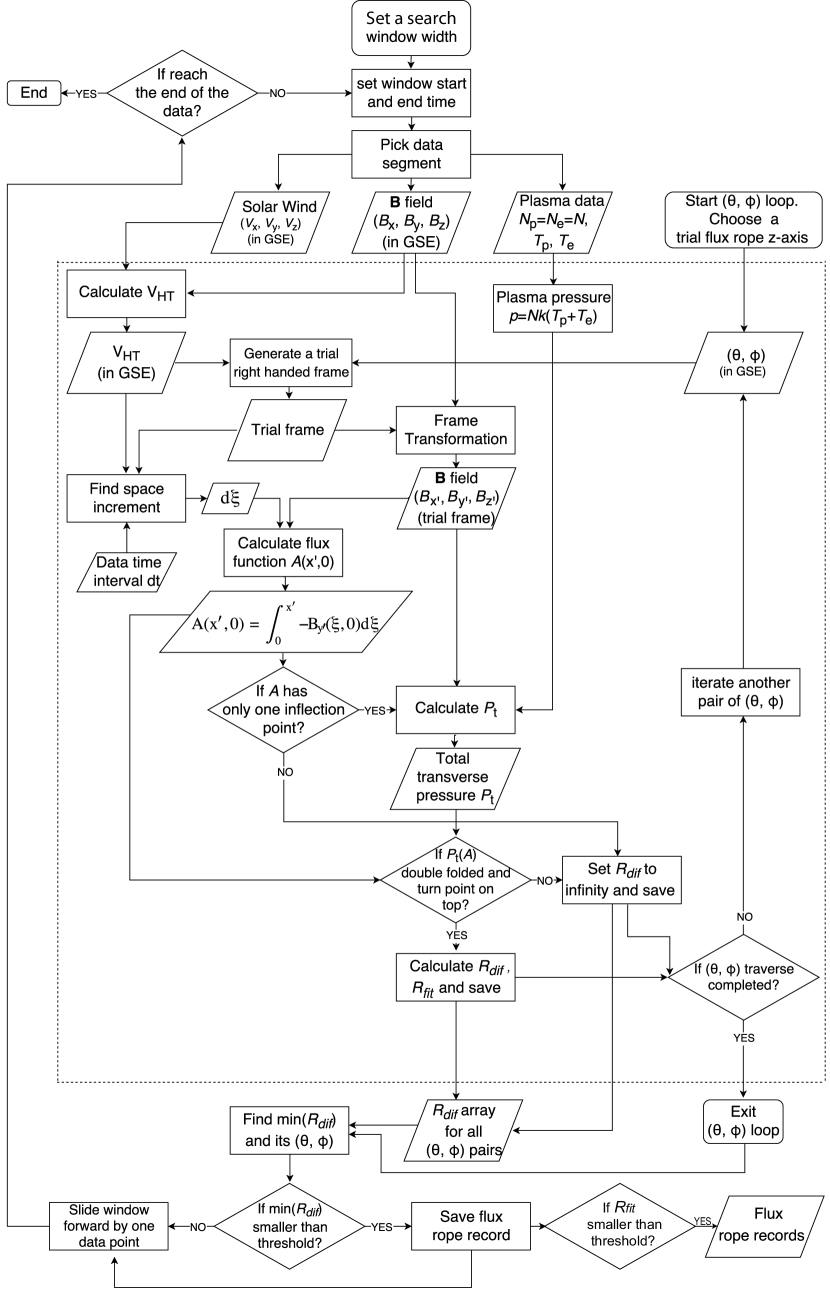
A flowchart with control flow and data flow (Figure 1) is prepared to show the detailed technical procedures. The flowchart illustrates the flux rope detecting process with a fixed window width for one of the iterations described earlier. The inner loop over directional angles $(\theta,\phi)$ is enclosed by the dashed lines, which shows the flux rope axial orientation determination process. The outer loop starting with the top rounded rectangle (“Set a search window width”) shows the sliding window process, which moves the window forward by one data point each time (by 1 minute in the present study) to scan the entire time series data.

A sliding window with the preset width is used to select data segment for analysis. The window width defines the maximum duration of the flux rope to be detected during this iteration. We also define a lower limit of the flux rope duration. The flux ropes only with their sizes between the lower and upper limits will be processed during this iteration. Subsequently we are going to run multiple iterations with different window widths to detect flux ropes with different sizes. Specifying the lower limit will avoid the duplication among the windows with different widths. For the time series magnetic field data within a given window, to make the $P_{t}$ versus $A$ curve double folded, the $A$ array must have one and only one inflection point (or turn point), defined as the place where the magnetic field component $B_{y^{\prime}}$ changes sign (see Equation 2) or equivalently the $A$ value reaches an extremum. As discussed in Section 2, since the transverse pressure $P_{t}$ is a single-valued function of $A$, the only way to make $P_{t}$ versus $A$ curve double folded is that the $A$ array has to fold onto itself so that the $P_{t}$ versus $A$ curve is split into two branches at the inflection point. If the $A$ array has more than one inflection point, the corresponding $P_{t}$ versus $A$ curve will be multiple folded, which may not meet the ground rule (2) for a single flux rope configuration. When such a situation occurs, the window may contain more than one flux rope structures. We just need to narrow down the window size to make it contain only one single flux rope structure. On the other hand, a narrow window cannot detect the flux ropes with the duration longer than the window width. Therefore, to detect flux ropes with different sizes, we have adopted the strategy of using multiple windows with different widths.

In the detection program, the number of inflection points is examined by checking the number of extrema of $A$ values in the data interval. The segments with more than one extreme $A$ values, excluding the boundaries, will be discarded. In practice, the local extrema in the $A$ array may be caused by measurement uncertainty or small fluctuations. To remove the effect of small local extrema, the smoothed $A$ array is used to check the number of inflection points. The third order Savitzky-Golay filter is applied to smooth the $A$ array. The width of the smoothing window needs to be specified for the Savitzky-Golay filter to apply the smoothing. If the smoothing window size is too small, smoothing process can not remove most of the small fluctuations. In this case, some real flux ropes with small fluctuations will be discarded due to their multiple inflection points. If the smoothing window size is too large, the smoothing process will force to remove the large local extrema, which will cause the low quality structures to be labeled as flux rope candidates. After extensive experiments, we have found that the one half of the lower limit associated with each search window width is an appropriate choice of width for its smoothing window. Because the smoothing window width in Savitzky-Golay filter needs to be an odd number, if the one half of the lower limit is not an odd number, we will round it up to the nearest odd number.

The core procedure, corresponding to the inner loop denoted in Figure 1, consists of the following two major steps:

• Step 1. As the sliding search window moves forward, we calculate the $A$ array along the projected spacecraft path (at $y^{\prime}=0$) by (the prime symbol denotes the trial coordinates for a trial flux rope $z$-axis)

  $$A(x^{\prime},0)=\int_{0}^{x^{\prime}}-B_{y^{\prime}}(\xi,0)d\xi.$$ (2)

  The spatial increment is converted from the temporal sampling interval via $d\xi=-\mathbf{V}_{HT}\cdot\hat{\mathbf{x}}^{\prime}dt$, where a constant frame velocity $\mathbf{V}_{HT}$ is taken as the usual deHoffmann-Teller frame velocity (Khrabrov & Sonnerup, 1998). The remaining flow $\mathbf{v}^{\prime}=\mathbf{V}_{sw}-\mathbf{V}_{HT}$ in such a co-moving frame of reference would generally become negligible, where the solar wind velocity $\mathbf{V}_{sw}$ is measured in the spacecraft frame, e.g., the Geocentric Solar Ecliptic (GSE) coordinates. In practice, to speed up the searching process and noting that there is little difference between $\mathbf{V}_{HT}$ and average solar wind velocity over the data segment, the latter is usually used in lieu of the former. Apparently the inflection point corresponds to the point along the spacecraft path where the field component $B_{y^{\prime}}$ changes sign and a point at which the extreme value in $A$ is reached. If we find the calculated $A$ array within the window is monotonic or has more than one distinct inflection points, we will do nothing but simply move the window forward by one data point. A monotonic $A$ array contains no extrema and can never lead to a double-folded $P_{t}$ versus $A$ curve. An $A$ array with more than one inflection points indicates that the current window may contain multiple flux rope structures. For the former situation, there is no further action needed to be done, and for the latter, a smaller size search window in another run will take care of it. Once an $A$ array with only one inflection point is discovered, the $A$ array will be split into two branches at the inflection point. Then the two branches will be trimmed to have the same $A$ values at the boundaries. Note that the trimming is not according to the number of data points, but is according to the $A$ value, because physically the boundary of a flux rope is identified by a flux surface with the same $A$ value. After trimming, the two branches may not have the same length, but must have the same or similar boundary $A$ values. After getting two branches of $A$ values with the same boundaries, we can calculate $P_{t}$ values corresponding to each $A$ value. With both $P_{t}$ and $A$ values obtained along the two halves of the spacecraft path, we can evaluate the agreement between the corresponding two sets of $P_{t}$ versus $A$ values.

• Step 2. The next step is to examine how well the two halves (branches) of the $P_{t}$ versus $A$ curve overlap. Before doing this, another check process can be performed to reduce the further workload. As a physical nature of the flux rope under consideration, the total transverse pressure $P_{t}$ must reach its maximum in the flux rope center. Reflected in the two branches of the $P_{t}$ versus $A$ curve, the turning point (corresponding to the inflection point in the $A$ array) must be on the top. We choose to remove the cases with turning points not on top. Taking into account the measurement uncertainty and small fluctuations, we introduce the tolerance. With tolerance, we require that the $P_{t}$ value at the turning point be in top 15% of all $P_{t}$ values. If the data segment would survive the check after undergoing all the aforementioned procedures, we are ready to obtain two more metrics as defined below to check the double-folding quality:

  $$R_{dif}=[\frac{1}{2N}\sum_{i=1}^{N}({(P_{t})}_{i}^{1st}-{(P_{t})}_{i}^{2nd})^{2}]^{\frac{1}{2}}/|\max(P_{t})-\min(P_{t})|,$$ (3)

  and

  $$R_{fit}=[\frac{1}{L}\sum_{i=1}^{L}(P_{t}(x_{i},0)-P_{t}(A(x_{i},0)))^{2}]^{\frac{1}{2}}/|\max(P_{t})-\min(P_{t})|.$$ (4)

  We determined that the conditions $R_{dif}\leq 0.12$ and $R_{fit}\leq 0.14$ could guarantee good flux rope quality while keeping a significant number of candidates.

Equation (3) is modified from Equation (5) in Hu & Sonnerup (2002), and Equation (4) is taken from Hu et al. (2004). The residue $R_{dif}$ represents the point-wise difference between two branches, in which both ${(P_{t})}_{i}^{1st}$ and ${(P_{t})}_{i}^{2nd}$ are calculated from observational data. We find the $A$ array and the corresponding $P_{t}$ array in the first branch, then use these $A$ values to look up the corresponding $P_{t}$ values in the second branch. If there is no correspondence in the second branch for some points in the first branch, we use linear interpolation to create a match. Then we repeat the same process for the second branch. Finally, each $P_{t}$ in one branch has a counterpart in the other branch. We insert the two interpolated $P_{t}$ arrays into Equation (3) to calculate $R_{dif}$. Only $R_{dif}$ alone is not sufficient to decide if a data segment is a good flux rope candidate or not, because a small $R_{dif}$ can only guarantee the good double-folding of the two branches of $P_{t}$ versus $A$ curves, no matter what the shape of the folded curve is. A reliable threshold for $R_{dif}$ is hard to set for acceptable flux rope candidates. To help with this, we obtain an additional fitting residue by using a 3rd order polynomial to fit the data points of $P_{t}$ versus $A$. This fitting ignores the time sequence of the data points and merges two branches into one. Its fitting residue is defined in Equation (4) and denoted as $R_{fit}$, where $P_{t}(x_{i},0)$ is calculated from measured data and $P_{t}(A(x_{i},0))$ is calculated from the fitting function. Note that, there is a fraction factor $1/2N$ in $R_{dif}$’s definition, but in $R_{fit}$’s definition, this factor is $1/L$. This is because in $R_{dif}$, the number of terms under the summation operator is only about half of the number in $R_{fit}$, i.e., $L\approx 2N$, if the two branches of $P_{t}$ versus $A$ curve have the same number of data points. We use two different factors to make the two metrics, $R_{dif}$ and $R_{fit}$, comparable in magnitude. However, the two branches of $P_{t}$ versus $A$ curve must have the same $A$ value range, but not necessarily have the same number of data points. In practice, even with the inclusion of these scaling factors, we still set different threshold values for $R_{dif}$ and $R_{fit}$. Besides the number of data points, the range of $P_{t}$ value may also affect $R_{dif}$ and $R_{fit}$. So we normalize $R_{dif}$ and $R_{fit}$ by the range $|\max(P_{t})-\min(P_{t})|$. In the flux rope searching process, we use only $R_{dif}$ to look for optimal $z$-axis orientation as illustrated in Figure 1. For a given data segment, the value $R_{dif}$ for each trial $z$-axis orientation is calculated, then the $z$-axis orientation with the minimum $R_{dif}$ is taken as the optimal axial orientation. With the determined optimal axial orientation, if both $R_{dif}$ and $R_{fit}$ satisfy our criteria, this data segment will be labeled as a flux rope candidate. The threshold values for $R_{dif}$ and $R_{fit}$ are selected empirically by examining thousands of data segments with double-folding features in $P_{t}(A)$, and are given in Table 1.

3.2 Cleanup and Post-Processing

When one sliding window process with one preset window width is finished, we will obtain one record list of identified flux rope intervals. However, this record list has many overlapped records or intervals. We use an example to illustrate how overlapping happens. We imagine a true flux rope starting from 8:00 am and ending at 10:00 am. When a sliding window with the width of 2 hours just covers the entire flux rope time range, this flux rope will be recognized and recorded. If the window moves forward and covers the time range from 8:05 am to 10:05 am, the detecting algorithm will likely recognize a flux rope from 8:05 am to 9:55 am (after trimming the two branches of $P_{t}$ versus $A$ curve). As the window moves on by one data point each time, as long as it still covers the turn point located in the middle of the flux rope interval from 8:00 am to 10:00 am (the largest flux rope), and the detected flux rope is longer than the lower limit, the program will pick a part of the largest flux rope as a new flux rope. These flux ropes share the same turn point, and we call them a flux rope cluster. To clean up such a cluster from the record list, we usually pick the segment with the smallest $R_{dif}$ value and discard the others. We have considered possible improvements to avoid the overlapping. One possible method is to move the entire sliding window out of the time range of a flux rope once it is detected. However, we cannot guarantee that the one we picked is the best one in a flux rope cluster. Eventually we decided to slide the search window continuously to guarantee the detection of the maximum number of flux ropes.

The other situation of overlapping occurs when additional iterations, i.e., additional lists of records, are completed. When all iterations with different window widths are finished, we need to combine all flux rope records. With the program setting introduced in the beginning of Section 3, we will end up with 70 event lists from 70 iterations. We cannot simply merge these lists into one, since a long flux rope may cover one or more short flux ropes from different lists. In fact, this is an interval scheduling problem in computer science. The optimal solution is to accommodate as many flux rope records as possible. We use the greedy algorithm to find the optimal solution. The main idea of the greedy algorithm in interval scheduling problem is to firstly accommodate the event with the earliest end time.

The cleanup procedures proceed with the following steps: 1) Clean the overlapped records in the event list with the longest flux rope duration. We sort the records by the flux rope end time. Firstly, find all the flux ropes that overlap with the first record, then keep the first flux rope and discard others. Then process the next record until all overlapped records are removed. This step results in a temporary list with “empty slots” in-between flux rope intervals. 2) Then we pick the suitable records from the event list with the second longest flux rope duration, and insert them into the corresponding slots. Each slot may contain some overlapping intervals. We still use the greedy algorithm illustrated in step 1) to accommodate them. 3) Continue with the next longest, and so on, until all flux ropes are accommodated.

The last check step is the standard Walén test to rule out possible Alfvénic structures (Paschmann & Sonnerup, 2008). An Alfvén wave or structure may show the similar magnetic field profile to a magnetic flux rope (e.g., Marubashi et al., 2010). The scale size of small-scale flux ropes is comparable with that of Alfvénic structures. We have to do further test to remove Alfvén waves from our flux rope database in order to comply with the GS equation in the present study. The Walén slope is defined as the slope of the linear regression line between the remaining flow velocity $\mathbf{v}^{\prime}$ in the co-moving frame of reference and the local Alfvén velocity, component-wise. We remove the records whose absolute value of Walén test slope is greater than or equal to 0.3 (indicating significant remaining flows in the reference frame co-moving with the structure). Up to this point, we have finished all major steps toward building the flux rope database. At last, we have the option to apply one more criterion. Considering that the average magnitude of magnetic field in the ambient solar wind is about 5 nT, we remove the flux rope records whose average magnitude of magnetic field $\bar{B}$ is less than 5 nT.

In summary, Table 1 lists the set of metrics and criteria we use in the identification of small-scale magnetic flux rope events from the in-situ Wind spacecraft measurements. The duration $9\sim 361$ minutes covers the range of most small-scale flux ropes, and this range is easily to be expanded to intermediate or large size flux ropes, e.g., with duration $6\sim 12$ hours or more, to bridge the gap between small-scale flux ropes and MCs. The condition $\bar{B}\geq 5$ nT excludes small fluctuations in the solar wind. The thresholds on the metrics $R_{dif}$ and $R_{fit}$ guarantee the good quality of small-scale flux ropes, complying with the GS equation. And the Walén test slope threshold condition ($\leq 0.3$) acts to remove the Alfvénic structures or waves in the present study.

Table 1: Small-scale Magnetic Flux Rope Detection Metrics and Criteria

Duration	$\bar{B}$	$R_{dif}$	$R_{fit}$	Walén test slope
$9\sim 361$ (minutes)	$\geq 5$ (nT)	$\leq 0.12$	$\leq 0.14$	$\leq 0.3$

Figure 2: A collage of selected plots available on the SSMFR database website for one particular event. (a) The $P_{t}$ versus $A$ data points along the 1st half (red dots) and the 2nd half (blue triangles) of the spacecraft path. (b) The Walén test plot: $\mathbf{v}^{\prime}$ versus the Alfvén velocity $\mathbf{V}_{A}$ in GSE components (colored dots). Dashed line marks the linear regression line with the slope and the correlation coefficient given in the legend. (c) The magnetic field components (in red, green and blue) projected onto the usual GSE (upper panel) and the local flux rope (lower) coordinates, respectively.

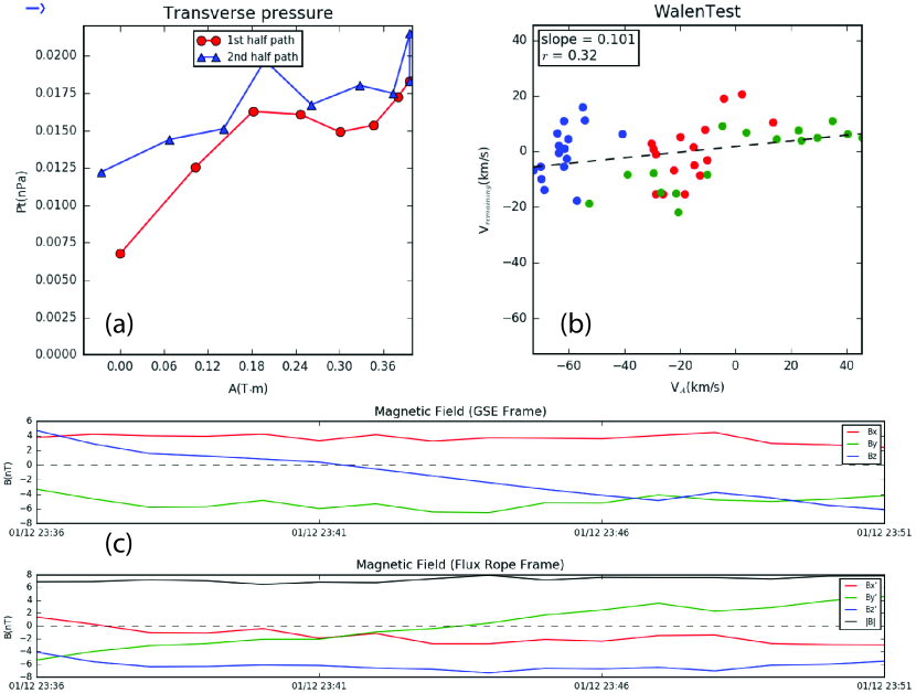
To conclude this section, we present an illustrative example for a particular event No. 181 in Year 2016 from the database website. Figure 2 shows the corresponding $P_{t}(A)$, Walén test and the magnetic field components plots directly extracted from the event web page. The flux rope interval spans the time period 2016/01/12 23:36 - 2016/01/12 23:51 UT with a duration 16 minutes. We also obtain the following parameters for the flux rope interval: $R_{fit}\approx 0.14$, $\bar{B}=7.25$ nT, $B_{max}=7.88$ nT, $\beta=\beta_{p}=0.94$, the average solar wind speed 537 km/s, the average proton temperature $T_{p}=0.28\times 10^{6}$K, and the optimal $z$-axis orientation $(\theta,\phi)=(80,140)$ degrees. The $z$-axis direction translates into GSE cartesian coordinates as a unit vector $(-0.7544,0.6330,0.1736)$. Figure 2 (a) shows the double-folding feature of $P_{t}(A)$ in which the 2nd half (branch) folds back onto the 1st one. The deviation between the two branches was evaluated by the two metrics and they fell below the thresholds given in Table 1. Figure 2 (b) shows the Walén test result with a slope 0.101 from the linear regression line. Figure 2 (c) shows the magnetic field components in the flux rope interval, especially in the lower panel, after projected onto the flux rope frame $(x^{\prime},y^{\prime},z^{\prime})$ for the optimal $z$-axis orientation determined. It shows a clear rotation in the $B_{y^{\prime}}$ component, and a unipolar axial field $B_{z^{\prime}}$, consistent with a flux rope configuration. For additional information, we encourage interested readers to explore the database website to learn about the variability and extensiveness of such an event database.

4 Small-scale Magnetic Flux Rope Database from Wind Spacecraft Measurements

We apply the flux rope detection algorithm based on the GS reconstruction technique to the Wind spacecraft measurements during 1996-2016, covering nearly two solar cycles. We successfully detected a large number of small-scale magnetic flux ropes with more general configurations, including non-force-free and non-axisymmetric configurations under the assumption of 2D quasi-static equilibrium. Table 2 lists the number of flux ropes detected by our algorithm in each year. There are a total number of 74,241 small-scale magnetic flux ropes detected, with an average number more than 3,500 per year. This database provides sufficient number of samples for interested researchers to carry out statistical analysis, correlate with other structures, and examine some special cases in detail.

(a)

(b)

Figure 3: (a) The monthly counts of flux rope events occurrence (left axis) and the monthly sunspot numbers (black curve; right axis) during 1996-2016. Colors represent counts of events with different duration as indicated. (b) The monthly flux rope total duration (left axis) and the monthly sunspot numbers (right axis) during 1996-2016. The format is the same as in (a). The sunspot numbers are courtesy of WDC-SILSO, Royal Observatory of Belgium, Brussels.

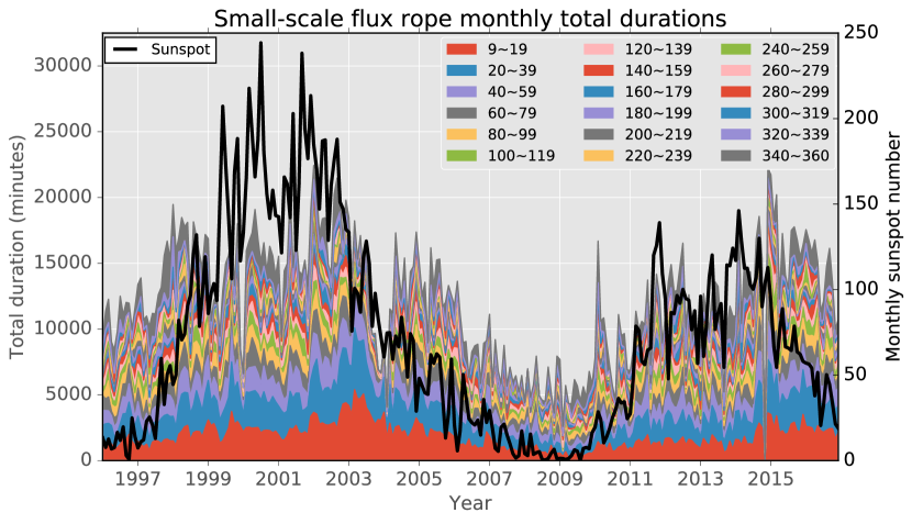
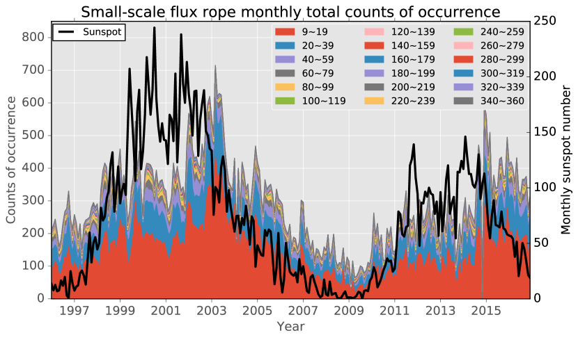
Figure 3 (a) shows the monthly occurrence counts of small-scale flux ropes from 1996 to 2016, covering solar cycles 23 (from May 1996 to December 2008), and 24 (which began in December 2008, reached its maximum in April 2014, and may have ended in early 2017). The different colors represent different duration of small-scale flux ropes (from 9 minutes to 360 minutes), and the thick black line is the corresponding monthly sunspot number. The events of smaller duration generally have greater rates of occurrence. Clearly the total counts including all events of variable duration follow the monthly sunspot numbers, hinting at solar-cycle dependency of these events. Note that the occurrence counts also vary cycle by cycle. From the sunspot numbers we can see that the solar activity in cycle 23 is more intense than that of cycle 24, and accordingly, the overall small-scale flux rope occurrence counts in cycle 23 are greater than those of cycle 24, approximately proportional to sunspot numbers. The peaks of occurrence counts tend to appear in the declining phase of each solar cycle. Figure 3 (a) shows variations in a way consistent with the change of magnetic cloud occurrence rate as shown by, e.g., Gopalswamy et al. (2015). During solar maximum, there are more events occurring, and there are fewer during solar minimum. One may argue that both magnetic clouds and small-scale flux ropes originate from solar eruptions, since they seem to share the similar dependency pattern with solar activity. However, this fact is still not a sufficient condition such that the small-scale flux ropes originate from the Sun. On one hand, there may be two populations of small-scale flux ropes that have different origins and different solar cycle dependencies, i.e., one population has solar cycle dependency but the other does not. When they are mixed, the solar cycle dependency may still appear. On the other hand, even if all small-scale flux rope events have solar cycle dependency as magnetic clouds do, we still cannot conclude that they originate from the Sun, since magnetic clouds have clear solar eruption correspondences but small-scale flux ropes do not. There may be other plasma dynamic processes far away from the Sun that could create these small-scale flux ropes and are also modulated by the solar activity cycle.

Figure 3 (b) is the monthly total duration for each group in (a) from 1996 to 2016. The format is the same as Figure 3 (a). In Figure 3 (b), the vertical axis represents the total small-scale flux rope duration in minutes for each similarly color-coded group. Although in the monthly duration plot, the area taken up by smaller flux ropes is suppressed, the solar cycle dependency shown in Figure 3 (a) still appears in Figure 3 (b). This plot shows that the solar cycle dependency is not only attributed to smaller flux ropes, but also to larger flux ropes. The sudden dips in event count and duration occur for the month of November 2014 due to a prolonged data gap, during which no event was identified.

Table 2: The Number of Detected Small-scale Magnetic Flux Ropes in Each Year

Year	1996	1997	1998	1999	2000	2001	2002	2003	2004	2005	2006
Counts	2787	2878	4182	4454	4425	4203	5930	6086	4229	4017	2620
Year	2007	2008	2009	2010	2011	2012	2013	2014	2015	2016	Total
Counts	2040	1620	1076	2209	2731	3051	2658	3690	4987	4368	74241

Figure 4: The home page of the small-scale magnetic flux rope database website.

4.1 On-line Database

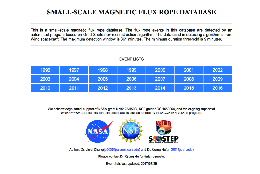
We have established a website (https://fluxrope.info) to host this database online. We make the database open to the public and keep it up to date. More flux rope events with longer duration and at higher latitude locations will be added in near future. Figure 4 is a snapshot of the home page of the small-scale magnetic flux rope database website. When clicking on any year on the “EVENT LISTS” table, the annual event list page will show up. The full table is available in machine readable format. Table 3 gives an example of its form and content. The event list page lists every detected flux rope event in one year in chronological order. For each flux rope record in each row, some basic characteristics are listed including the time range in UT, duration in minutes, fitting residue ($R_{fit}$), average magnetic field strength, maximum magnetic field strength, average plasma $\beta$, average proton plasma $\beta_{p}$, average solar wind speed $\overline{V}_{sw}$, average proton temperature, and flux rope axial orientation. More information on magnetic field and plasma profiles is stored offline and can be put online in new versions of the website. These quantities make it very convenient for us and other researchers to further apply more selection criteria to pick desirable subset of events for different purposes.

Table 3: Flux rope events

Column	Label	Explanation
1	Num	Index identifier
2	Start	Observation start; mm/dd/yyyy hh:mm
3	End	Observation end; mm/dd/yyyy hh:mm
4	Time	Observation duration
5	$R_{dif}$	Residue, see text
6	$<B>$	Average magnetic field strength (nT)
7	Bmax	Maximum magnetic field strength (nT)
8	$<{\beta}>$	Average plasma beta value
9	$<{\beta}_{p}>$	Average proton beta value
10	Vsw	Solar wind velocity (km/s)
11	$<T_{p}>$	Average proton temperature (MK)
12	$\theta$	Polar angle (deg)
13	$\phi$	Azimuthal angle (deg)
14	zAxis0	Z-axis orientation
15	zAxis1	Z-axis orientation
16	zAxis2	Z-axis orientation
17	Size	Scale size (AU)
18	$N_{p}$	Mean proton number density (cm-3)
Table 3 is published in its entirety in the electronic edition
of the Astrophysical Journal. A portion is shown here
for guidance regarding its form and content.

The time range for each record is a clickable hyperlink which will navigate to the detailed flux rope information page which is demonstrated in part in Figure 2 for one particular event. They help judge the “double-folding” quality of $P_{t}(A)$, and the result from the Walén test. Generally speaking, a spread of the data points horizontally in the latter plot indicates satisfaction of the detection criterion based on the magnetohydrostatic theory. Additionally, the usual hodograms of the flux rope magnetic field components from the MVAB are also displayed, which visualizes the movement of the end points of magnetic field vectors. Generally a smooth rotation in one or two magnetic field components, typical of a flux rope configuration, may be inspected in these plots. Such signatures consistent with a flux rope configuration are further displayed in panels of various time series data of magnetic field and solar wind parameters, complemented with the pitch angle distribution of suprathermal electrons, the temperature of protons and electrons, when available, and plasma $\beta$, etc.

This website provides a large number of small-scale magnetic flux rope events and a good deal of associated information, which can benefit the relevant studies on these and other structures in the solar wind. Before we delve into detailed statistical analysis, we show the basis for an usual classification of events, based on the solar wind speed.

Figure 5: The histogram of average solar wind speed within each small-scale flux rope interval.

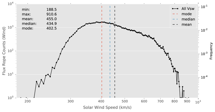
Figure 5 is the histogram of average solar wind speed $\overline{V}_{sw}$ within each flux rope interval. One can see a peak near $\overline{V}_{sw}=$400 km/s (the mode of the distribution is 402 km/s) and three approximately linear sections in the curve with different slopes on this log-log plot. The first section of the curve is from $\overline{V}_{sw}=$200 km/s to $\overline{V}_{sw}=$400 km/s. The slope of the first section is positive. The second section of the curve is from $\overline{V}_{sw}=$400 km/s to $\overline{V}_{sw}=$650 km/s, with a negative slope. The third section of the curve is from $\overline{V}_{sw}=$650 km/s to $\overline{V}_{sw}=$900 km/s, with a steep negative slope. Three distinct slopes in log-log plot indicate three distinct power law distributions with different power indices. Since the solar wind speed is a key factor in space plasma dynamic processes, different power law distributions may imply different physical processes involved in different plasma flow streams. Therefore, in the following analysis, we split the entire event database into two subsets according to the corresponding average solar wind speed either greater or less than 400 km/s. Note that this value is nearly identical to the mode of the distribution, 402 km/s, corresponding to the peak in the distribution of average solar wind speed (Figure 5).

Figure 6: The 2-D histogram of flux rope average solar wind speed ($\overline{V}_{sw}$) $versus$ scale size.

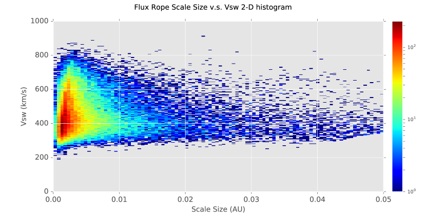
Figure 6 is the 2-D histogram of flux rope $\overline{V}_{sw}$ $versus$ scale size. It shows that the flux ropes with larger scale sizes tend to appear in slow solar wind ($\overline{V}_{sw}<$400 km/s), and for the smaller scale size flux ropes, the solar wind speed associated with them spreads widely (from $\sim$ $\overline{V}_{sw}=$200 km/s to $\sim$ $\overline{V}_{sw}=$800 km/s). The line of $\overline{V}_{sw}=$400 km/s divides the plotted shape into two triangles. Above the line of $\overline{V}_{sw}=$400 km/s, the solar wind speed goes down as the scale size becomes large, while below the line of $\overline{V}_{sw}=$400 km/s, the solar wind speed goes up as the scale size increases. This plot is another basis based on which we split the entire event set at $\overline{V}_{sw}=$400 km/s.

4.2 Statistical Results of Flux Rope Properties

As discussed in Section 1, there is a long-standing debate on the origination of small-scale magnetic flux ropes. In this section, we are going to present some statistical analysis of the flux ropes properties based on our database in the hope of shedding some light on the origin of these structures in the solar wind.

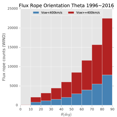
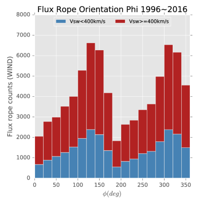
Figure 7 (a) and (b) show the histograms of the small-scale flux rope axial orientations in the GSE spherical coordinates based on the last column of the event list. Figure 7 (a) is the polar angle histogram which is binned by $10^{\circ}$, and Figure 7 (b) is the azimuthal angle histogram which is binned by $20^{\circ}$. These two plots indicate that the small-scale flux ropes located near the ecliptic plane have preferential axial orientations. From Figure 7 (a), one can see that the distributions are skewed toward large polar angels, i.e., most of them tend to lie on the ecliptic plane. Figure 7 (b) shows two peaks located at bin $120^{\circ}\sim 140^{\circ}$ and the bin $300^{\circ}\sim 320^{\circ}$. In fact, these two bins represent two parallel but opposite directions in the GSE $XY$ plane, so they differ by about $180^{\circ}$. Either one of these directions happens to be the tangential direction of the Parker spiral at 1 AU (corresponding to $\phi\approx 135^{\circ}$ or $315^{\circ}$). This indicates that the projection of the flux rope axis tends to align with the Parker spiral direction on the ecliptic plane. The red and blue bars represent the events occurring under different solar wind speed conditions (blue: $\overline{V}_{sw}<$ 400 km/s; red: $\overline{V}_{sw}\geq$ 400 km/s). Figure 7 (a) and (b) indicate that the small-scale flux ropes have similar orientation preferences in both fast and slow solar wind in the ecliptic.

(a)

(b)

Figure 7: (a) Flux rope axial orientation: polar angle $\theta$ histogram. The actual polar angle range is from $0^{\circ}$ to $180^{\circ}$. We restrict end points of the direction vectors in the upper hemisphere, and do not distinguish the vectors with opposite directions from each other. (b) Flux rope axial orientation: azimuthal angle $\phi$ histogram. This angle is measured from the positive GSE-$X$ axis toward the projection of the flux rope axis onto the ecliptic plane.

(a)

(b)

Figure 8: (a) The histogram of small-scale flux rope duration plotted in logarithmic scales. The time range is from 9 minutes to 361 minutes, with 5 minutes bin size. Note that the high tails to the right ends of the curves are due to duration boundary cutoff effect (see explanations in text). (b) The histogram of small-scale flux rope cross section scale sizes plotted in logarithmic scales, with 0.00025 AU bin size. The flux rope scale size is calculated from the flux rope duration taking into account the axial orientation. Again, the low points to the left and right ends of the curves are due to boundary cutoff effect (see explanations in text). For both (a) and (b), the basic statistical quantities and linear regression parameters for each curve are listed, respectively.

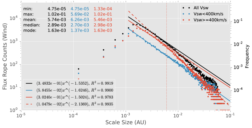
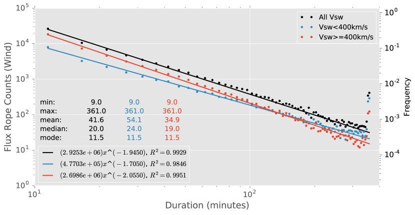
Figure 8 (a) and (b) show the duration and scale size distributions of small-scale flux ropes in our database. The data points in black in each plot represent the histograms of the entire event set, and the points in blue or red represent the histogram of the the subsets for slow ($\overline{V}_{sw}<$400 km/s) and fast ($\overline{V}_{sw}\geq$400 km/s) solar wind speed, respectively. In Figure 8 (a), the shapes of these three curves are close to straight lines on the log-log scale except for the high tails to the right. After examining the generation process of our flux rope database, we find that the high tail is due to cutoff effect of a finite range of window widths. As described in Section 3, the last step of the flux rope detecting process is to combine all flux rope candidate lists with different duration ranges. In this process, some short duration flux ropes will be absorbed into the longer duration flux ropes which enclose them. In the present database, the longest duration range is 354$\sim$361 minutes, which means that the flux ropes within this duration range will not be merged into longer flux ropes, since there is no longer duration allowed beyond this range, thus resulting in the cutoff. This cutoff leads to the enhanced fluctuation and a high tail near the end to the right, corresponding to the last duration range in the current search. To confirm this effect, we manually shifted the cutoff boundary to shorter duration, the high tail also shifted accordingly. In Figure 8 (b), there are low tails at both ends in each curve, which are also caused by the same cutoff effect of finite duration ranges. Due to the boundary cutoff in duration ranges, when converting the duration to scale size, there is a lack of events near the lower and upper scale size boundaries as shown. We exclude these abnormal sections of the data points in the subsequent analyses.

Except for the high tails due to the cutoff effect, Figure 8 (a) shows a linear relation between the flux rope occurrence counts and the duration under logarithmic scales, which indicates a power law distribution of flux rope duration. The color coded straight lines are the corresponding fitted power law functions as denoted. The flux ropes under the slow solar wind condition obey the power law with a power index $\sim-1.70$, while the ones in fast solar wind obey the power law with power index $\sim-2.06$. One can see that the red curve ($\overline{V}_{sw}\geq$400 km/s) has larger absolute slope value than the blue curve ($\overline{V}_{sw}<$400 km/s). The intersection of the blue and red curves is located at about 100 minutes. To the left side of the intersection point, there are more flux rope events in fast solar wind, while to the right, there are more flux rope events with low solar wind speed. This indicates that the longer duration flux ropes (duration$>$100 minutes) tend to occur under the slow solar wind speed condition.

Figure 8 (b) also exhibits approximately linear relations (in logarithmic scales) between flux rope scale size and occurrence counts, excluding the low ends due to the cutoff effect. This indicates a power law distribution of flux rope scale sizes, properly calculated taking into account the axial orientations. At a glance, the absolute slope of the red curve ($\overline{V}_{sw}\geq$400 km/s) seems to be greater than that of the blue curve ($\overline{V}_{sw}<$400 km/s), especially for the section of larger scale sizes. Comparing with Figure 8 (a), one can see that the flux ropes ranging from 9$\sim$361 minutes have the approximately corresponding scale-size range of 0.002$\sim$0.05 AU (excluding the lower end). When we use power law functions to fit the data, we find that the data points in blue color are fitted very well by a single power function with power index $\sim-1.62$, but for the red and black data points, the tails show noticeable deviations from single fitted lines. Apparently, the deviations in the black data points are due to the deviations in the red ones. We use two power law functions with different power indices to fit the red data points, and find that in the scale size range $0.001\sim 0.01$ AU, the red data points are well fitted by a power law function (solid line) with a power index $\sim-1.50$, while in the range $0.01\sim 0.05$ AU, the red data points are well fitted by a power law function (dashed line) with a power index $\sim-2.14$. The breakpoint of the two power laws is at $\sim 0.006$ AU.

It is interesting to note that both Figure 8 (a) and (b) obey the power law distribution. The power law distributions are fairly common in nature. These analysis results are relatively new, concerning these small-scale flux ropes from a large sample. We will discuss these results in the following from the perspective of self-organized criticality theory.

The self-organized criticality (SOC) theory was first proposed by Bak et al. (1987), and then applied by Lu & Hamilton (1991); Lu et al. (1993) to solar physics to explain the power law distributions of flare occurrence rate over flare energy, peak flux, and duration. This model is usually referred to as the avalanche model and has been widely used to explain the statistical characteristics of hard x-ray (HXR) flares (Lu et al., 1993; Vlahos et al., 1995; MacKinnon & MacPherson, 1997; Georgoulis & Vlahos, 1998). The avalanche model predicts a power law distribution for the total energy, the peak luminosity, and the duration of individual events. Li et al. (2016) studied the solar flares and CMEs during the solar cycle 23. They found that the solar flare duration distribution obeys a power law with a power index $\sim-2.55$. In Figure 8 (a), we also produce a power law with an index close to -2 for all events (black line), implying that the occurrence of small-scale flux ropes may be explained by SOC theory. Note that the absolute values of the power indices from our fitted functions are generally smaller than those in Li et al. (2016), indicating solar flares or CMEs and small-scale flux ropes are probably corresponding to two different kinds of processes. Although they share the similar statistical characteristics in terms of the power law distributions in certain properties, complying with the SOC theory, the underlying physical mechanism responsible for generating such behavior still cannot be revealed.

(a)

(b)

Figure 9: (a) The histogram of average proton temperature within flux ropes in logarithmic scales, with 0.005 ($10^{6}$ K) bin size. (b) The histogram of average proton number density within flux ropes in logarithmic scales, with 0.2 $\#/cc$ bin size. For both (a) and (b), the blue curve represents the flux rope events with solar wind speed $\overline{V}_{sw}<$400 km/s, and the red curve with solar wind speed $\overline{V}_{sw}\geq$400 km/s. The black curve represents the entire event set.

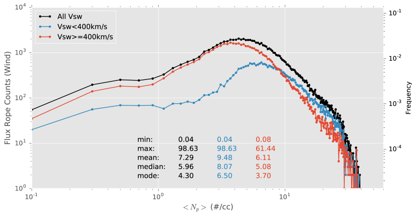
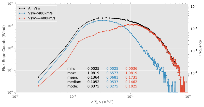
Figure 9 (a) is the histogram of average proton temperature within flux ropes plotted in logarithmic scales. We can see that the peaks of blue and red curves are separated, corresponding to different modes. The peak of the red curve ($\overline{V}_{sw}\geq$400 km/s) is near $\overline{T}_{p}$ $\approx$ 0.1 ($10^{6}$ K), while the peak of the blue curve ($\overline{V}_{sw}<$400 km/s) is near $\overline{T}_{p}$ $\approx$ 0.03 ($10^{6}$ K). Therefore, the small-scale flux ropes in low speed solar wind ($\overline{V}_{sw}<$400 km/s) tend to have low proton temperature, while the ones under medium and high speed solar wind ($\overline{V}_{sw}\geq$400 km/s) tend to have high proton temperature. Note that the black curve and the red curve are overlapping beyond $\overline{T}_{p}$ = 0.2 ($10^{6}$K), which means that the small-scale flux ropes with proton temperature greater than 0.2 ($10^{6}$ K) occur dominantly under medium and high speed solar wind conditions. Figure 9 (b) is the histogram of average proton number density within flux ropes plotted in logarithmic scales. Note that the appearance in Figure 9 (b) is opposite to that in Figure 9 (a). In Figure 9 (b), the flux ropes with medium and high solar wind speed tend to have lower proton number density while the flux ropes in slow solar wind tend to have higher density. To summarize Figure 9 (a) and (b), the flux ropes in slow speed solar wind tend to have low proton temperature and high proton number density, while the flux ropes in medium and high speed solar wind tend to have high proton temperature and low proton number density.

(a)

(b)

Figure 10: (a) The histogram of average plasma $\beta$ within flux ropes, with bin width 0.01. (b) The histogram of average proton $\beta_{p}$ within flux ropes, with bin width 0.01. For both (a) and (b), the blue curve represents the flux rope events with solar wind speed $\overline{V}_{sw}<$400 km/s, and the red curve with solar wind speed $\overline{V}_{sw}\geq$400 km/s. The black curve represents the entire event set.

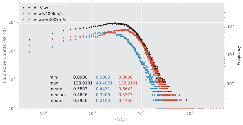
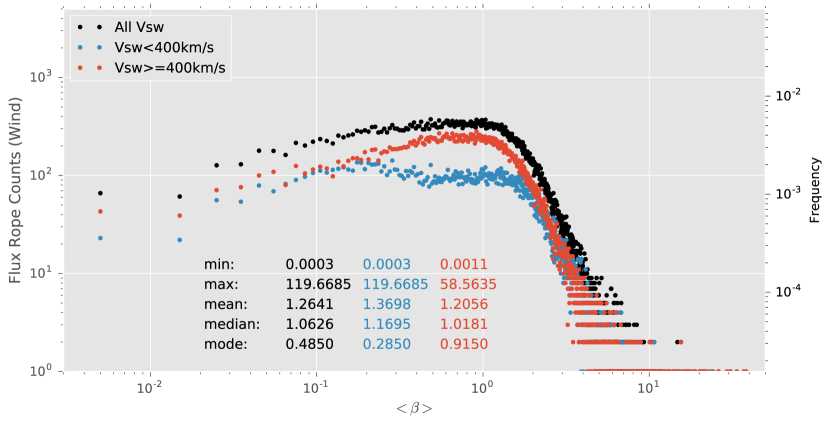
Figure 10 (a) is the histogram of average plasma $\beta$ (electron temperature $T_{e}$ included) within flux ropes plotted in log-log scales. The black curve shows that the occurrence peak of all small-scale flux ropes is close to $\overline{\beta}=1$. The red curve has the same trend as the black curve, while the blue curve has a flat top. From the shapes of these curves, and especially the medians, we find that the numbers of small-scale flux rope with $\overline{\beta}<1$ and the ones with $\overline{\beta}>1$ are about the same. However, in magnetic clouds, the magnetic pressure always dominates over thermal pressure, which causes ultra low plasma $\beta$. Figure 10 (b) is the histogram of average proton plasma $\beta_{p}$ (excluding $T_{e}$) within flux ropes plotted in log-log scales. Because the electron temperature data quality is generally poor, they are not always available. To overcome the large data gaps in $T_{e}$, we also plot the histogram of the average proton plasma $\beta_{p}$, in which only the contribution of protons temperature $T_{p}$ is included when calculating the thermal pressure. Figure 10 (b) shows the similar distributions as Figure 10 (a). All curves in Figure 10 (b) are shifted to the left compared with Figure 10 (a), indicating that the plasma $\beta$ is significantly enhanced by the electron temperature contribution, as also indicated by the various statistical quantities denoted on each plot.

Figure 11: The 2-D histogram of flux rope proton temperature $versus$ scale size. The bin grids are 200$\times$200. Subplots (a) to (e) are histograms under different solar wind speeds as denoted, and subplot (f) is the histogram for the entire event set. The color bar represents the small-scale flux rope counts.

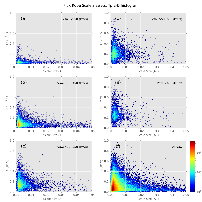
The low proton temperature ($T_{p}$) is a key characteristic of magnetic clouds. However, for small-scale magnetic flux ropes, the $T_{p}$ varies case by case. Figure 11 is the 2-D histogram of flux rope $T_{p}$ $versus$ scale size. The triangle shape distribution stretching down to the right in Figure 11 (f) indicates that the flux ropes with larger scale size ($\geq 0.02$ AU) usually have lower $T_{p}$ ($\leq 0.1$ $\times 10^{6}$ K). Given that the large-scale magnetic flux ropes (MCs) have low $T_{p}$, there seems to be a smooth transition from the small-scale magnetic flux ropes to their larger counterparts. For the smaller size small-scale flux ropes, the range of $T_{p}$ spreads widely. Figure 11 (f) shows that the range of $T_{p}$ of the flux ropes with scale size less than 0.05 AU spreads from near 0 to 0.8 ($10^{6}$ K). When looking into the distribution under different solar wind speed conditions, we find that most of the relatively larger size small-scale flux ropes ($\geq 0.02$ AU) appear in the slow solar wind with low $T_{p}$ (see Figure 11 (a), (b), and (c)). As for the relatively smaller size small-scale flux ropes ($\leq 0.01$ AU), they appear in both fast and slow solar wind. The different locations of the high frequency regions (in red and yellow colors) in each subplot ( Figure 11 (a) $\sim$ (e)) show that the flux ropes in high (low) speed solar wind tend to have higher (lower) proton temperature, which is consistent with the result shown in Figure 9 (a).

4.3 Cycle-to-cycle Variations

Gopalswamy et al. (2015) investigated the correlation between the annual number of magnetic clouds events and the frontside halo CMEs, and compared both with the sunspot numbers. They found significant difference in the properties of MCs between solar cycles 23 and 24. It is natural to perform a similar analysis on the small-scale flux ropes by simply repeating the above statistical analyses on the two cycles separately. Unlike the findings of Gopalswamy et al. (2015), who compared the MC properties and their geo-effectiveness for the past two solar cycles and concluded that significant differences were found, we conducted a similar analysis by comparing the statistics of the same set of parameters between the two solar cycles. We do not find any noticeable differences among the majority of parameters, except for the following two quantities: the average field magnitude and the average plasma $\beta$, within each flux rope interval. For example, Figure 12 shows the distributions of selected parameters for each cycle separately. Little difference is seen between the two cycles.

Figure 12: The histograms of (a) duration, (b) scale size, (c) axial orientation angle $\theta$, and (d) $\phi$ of small-scale flux rope events for the solar cycles 23 and 24.

Figure 13: The histograms of (a) average $\beta$ and (b) average magnetic field magnitude within small-scale flux rope intervals for the solar cycles 23 and 24.

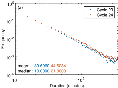
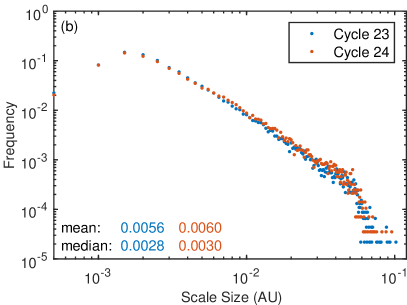
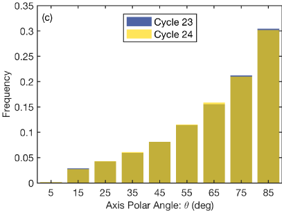
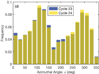
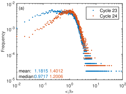
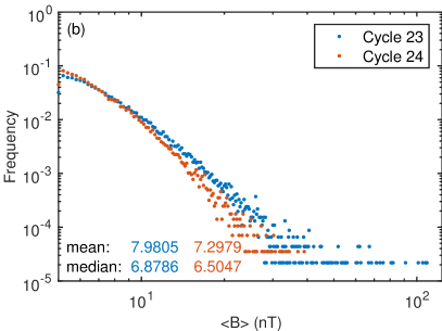
Figure 13 shows the histograms of the average plasma $\beta$ and the average magnetic field magnitude for solar cycles 23 and 24, respectively. The overall distributions are similar for the two cycle. For solar cycle 23, the plasma $\beta$ has slightly higher mean and median values than cycle 24. Correspondingly the average field magnitude has a smaller mean in cycle 24, and does appear to be weaker as shown in Figure 13 (b). These variations can be explained by the known cycle-to-cycle variation in the interplanetary magnetic field magnitude because the cycle 24 has a weaker magnetic field magnitude than cycle 23 (e.g., Zhao et al., 2018a).

5 Waiting Time Distributions

The waiting time distribution (WTD) is defined by the distribution of time intervals or separations between discrete events. The WTD of the successive discrete events reveals whether they occur independently. Many models on solar eruptive processes predict definitive WTDs, so the WTD analysis based on observational data is a powerful tool to validate these models. The WTD analysis is widely used in analyzing space plasma processes such as CMEs (Li et al., 2016), solar flares (Wheatland et al., 1998; Li et al., 2016), current sheets (Miao et al., 2011), gamma ray burst (Wang & Dai, 2013), and solar energetic particles (Li et al., 2014), and also in other discrete time random processes such as earthquakes (Sotolongo-Costa et al., 2000). In this section, we apply the WTD analysis on the occurrence of small-scale magnetic flux ropes, in order to investigate the underlying mechanism governing the flux rope origination process. We discuss the possible implications on the flux rope origination by comparing the WTDs of flux ropes with the WTDs of some relevant processes, especially those from the analysis of current sheets (Bruno et al., 2001; Greco et al., 2008, 2009a; Miao et al., 2011). Part of the analysis results from the flux rope wall-to-wall time distribution had been reported in Zheng & Hu (2018), which will not be repeated here.

As predicted by the avalanche model (Bak et al., 1987; Lu & Hamilton, 1991; Lu et al., 1993), the occurrence of solar flares is a Poisson process, i.e., the flare WTD is a simple exponential function in waiting time, $\Delta t$. In fact, the occurrence rate of many processes is non-constant, and as an observational result, the flare WTD usually shows time-dependent Poisson distributions (Wheatland, 2000; Aschwanden & McTiernan, 2010; Guidorzi et al., 2015; Li et al., 2016). However, some observational results showed the deviations of flare WTD from a simple Poisson process. Pearce et al. (1993) studied 8319 HXR solar flares during solar minimum (1980$\sim$1985), and pointed out that the WTD ($\Delta t$ ranging from 0 to 60 minutes) of flares has large deviation from a stationary Poisson process, but is well fitted by a power law function with a power index -0.75 (See Figure 4 in Pearce et al. (1993)), indicating that flares did not occur purely randomly. Li et al. (2016) investigated the statistical properties of CMEs and solar flares during solar cycle 23. They adopted the non-stationary Poisson distribution functions from Li et al. (2014) and Guidorzi et al. (2015) to fit the WTDs of solar flares and CMEs, and obtained good fitting results. In Li et al. (2014); Guidorzi et al. (2015) the non-stationary Poisson distribution functions and the asymptotic behavior of the longer waiting time near the tail lead to power law functions.

In this section, we try various fitting functions mentioned above to fit the flux ropes WTDs. Primarily we use exponential and/or a power law function fittings as we present below, which yields the optimal outcome. The functions used by Li et al. (2014); Guidorzi et al. (2015) do not work, partially due to the limited range of waiting time, $\Delta t$, in out database. Here we use two different kinds of definition for waiting time (e.g., Greco et al., 2009b). The first kind of waiting time is defined by the elapsed time from the end of one flux rope to the start of the next one, i.e., the time interval between adjacent flux ropes. And the second kind of waiting time is defined by the elapsed time from the starting time of one flux rope to the starting time of the next, i.e., the time interval between the starting times of two successive flux ropes.

Figure 14: The waiting time distribution (1st kind) of small-scale magnetic flux ropes. In this plot, the waiting time is defined by the interval between the end time of one flux rope to the start time of the next one. The dots in black represent the entire event set, and the dots in blue and red represent the subsets with low solar wind speed ($\overline{V}_{sw}<$400 km/s) and medium as well as high solar wind speed ($\overline{V}_{sw}\geq$400 km/s), respectively. The bin size is 5 minutes, and the data point for each bin is located in the bin center. The dashed lines are fitted curves by exponential functions, and the solid lines are fitted curves by power law functions. The dotted vertical line denotes the break point, which is located at 60 minutes. The statistical quantities and fitting parameters are denoted, where the function forms and the fitting quality metrics $R^{2}$ are listed.

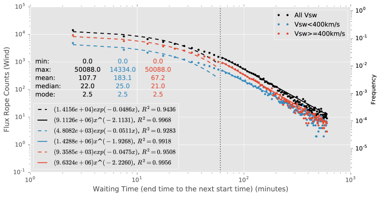
Figure 14 is the flux rope WTD of the first kind. For each color-coded data set, we use an exponential function to fit the data points with waiting time less than 60 minutes. The exponential function fits the data well where waiting time is less than 40 minutes. Then the deviation grows as the waiting time becomes larger. The section beyond 60 minutes is fitted by a power law function. The power law function fits the tail very well, with the coefficient of determination $R^{2}>0.99$ for each data set. An exponential WTD indicates a random Poisson process of the event occurrence, while a power law WTD suggests the clustering behavior of the events. The fitting results show that the overall WTD shown in Figure 14 is neither a simple Poisson distribution nor a power law distribution.

Figure 15: The waiting time distribution (2nd kind) of small-scale magnetic flux ropes. In this plot, the waiting time is defined by the interval between the start time of one flux rope to the start time of the next one. The format is the same as in Figure 14. The vertical dotted line is at 80 minutes.

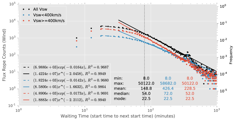
Considering that the starting time of one flux rope may correspond to the onset of solar eruptive process back on the Sun, according to the definition by Wheatland (2000), we perform the WTD analysis based on an alternative definition of waiting time. In this definition, the interval between two consecutive starting times is considered as the waiting time. We call the WTD under this definition the WTD of the second kind. Figure 15 shows the flux rope WTD of the second kind. One can notice the outliers near the two ends. The outliers on the tail locate between 300 minutes to 400 minutes, which is the same location as the outliers appearing in Figure 8 (a) and (b). Apparently, these outliers are due to boundary cutoff effect since the flux rope duration contributes to the waiting time of the second kind. As for the the outliers with the shortest waiting time, we also attribute them to boundary cutoff effect. Because in our database, the minimum flux rope duration is set at 9 minutes, there are no flux rope events with duration less than 9 minutes. However, the separation between two flux ropes can be of any time length. When we use the definition of the first kind, the shortest waiting time can be zero, but for the definition of the second kind, the shortest waiting time has to be 9 minutes. As a result, there is a lack of events with short waiting time in the WTD of the second kind. Excluding these abnormalities, we apply the same fitting approach as in Figure 14. In Figure 15, for each curve, we can see that the section less than 80 minutes is well fitted by an exponential function, and the section greater than 80 minutes is well fitted by a power law function. The exponential fittings in Figure 15 are better than those in Figure 14, indicating that the events associated with short waiting time ($<80$ minutes) are subject to the simple Poisson process, while the ones associated with longer waiting time ($>80$ minutes) seem to have clustering behavior. The combination of an exponential and a power law distribution implies there may be two distinct mechanisms responsible for the event occurrence.

It is worth noting that the fitting result given in Figure 15 is similar to the result on current sheets WTD obtained by Bruno et al. (2001); Miao et al. (2011). Bruno et al. (2001) showed an exponential fitting to the waiting time of intermittent events (current sheets) identified from the Helios 2 spacecraft measurements at 0.9 AU in a high speed stream. The exponential fit persisted for a range of waiting time between 12 minutes and $\sim$ 2 hours, compatible with the exponential-fitting range of $\Delta t$ in Figure 15. Miao et al. (2011) studied the statistical characteristics of current sheets observed by Ulysses in 1997, 2004, and 2005 (also including a few days in 1996 and 2006). They found that the current sheets WTD can be well fitted by an exponential function and a power law function as well. However, the break point in Miao et al.’s fitting is at $\sim e^{10}$ seconds (367 minutes) (see Figure 9 in Miao et al. (2011)), and the power law index is -1.85, which is different from the power law index in our results. A word of caution is that Miao et al.’s results were obtained from Ulysses observations near the ecliptic plane, but at radial distances $\sim$ 4-5 AU from the Sun. Therefore significant evolution, at least passively, has occurred between the two sets of results. Although not totally comparable, the similar piecewise behaviors of the flux rope WTD and the current sheet WTD imply that they may share similar generation mechanisms or have some kind of association.

Greco et al. (2009a, b) showed the consistency between the WTDs of the solar wind discontinuities observed by the ACE spacecraft at 1 AU and the corresponding WTDs of intermittent structures (current sheets) from the MHD turbulence simulations, suggesting that the solar wind magnetic structures may be created locally by MHD turbulence. Here the structures referred to by Greco et al. consist of “small random currents”, “current cores” (i.e. flux ropes), and “intermittent current sheets” (Greco et al., 2008, 2009a). In their study, the WTD of MHD simulation result agrees well with the WTD of ACE observational data in the short waiting time range ($<50$ minutes, the correlation length scale of solar wind turbulence). For the departure from the power law beyond 50 minutes, they attributed that to the limited length scales, thus no large-scale features allowed in the MHD simulations. In general space plasma scenario, the current sheets can be considered as boundaries of flux ropes with negligible thickness. To make a direct comparison with the WTD of current sheets in Greco et al.’s study (Greco et al., 2009a, b), where current sheets were identified with zero thickness, we provide a proxy to those current sheets from our small-scale magnetic flux rope database. Considering that the flux ropes are bounded by current sheets, we can assume that there are current sheets existing at the starting time and the end time of each flux rope interval. We call these current sheets flux rope “walls”. Then the time interval between adjacent walls can be considered as a proxy to the waiting time of current sheets. We showed in Zheng & Hu (2018) the consistent results agreeing with Greco et al. (2009b) in terms of the wall-to-wall time (equivalent to the waiting time of current sheets) and axial current density distributions from our GS-based analysis of small-scale magnetic flux ropes. Such analysis provided the direct evidence, through our unique approach, in supporting the view of locally generated coherent structures intrinsic to the dynamic processes in the solar wind as manifested either by magnetic reconnection or turbulence cascade.

6 Locations of SSMFR with Respect to the HCS

The argument that the small-scale magnetic flux ropes are created locally is partly based on the fact that some events were found near the heliospheric current sheet (HCS). Upon the first discovery of small-scale flux ropes, Moldwin et al. (1995) interpreted their findings in terms of multiple magnetic reconnection of previously open field lines at the HCS. Later, Moldwin et al. (2000) reported several additional small-scale flux ropes observed by both IMP 8 and Wind spacecraft. They suggested that these small-scale flux ropes were created in the HCS instead of the solar corona because of the following reasons: (1) bimodal size distribution, (2) lack of expansion, (3) different plasma characteristics, and (4) similar radial scale size with estimated HCS thickness. Cartwright & Moldwin (2010) studied the distribution of small-scale flux ropes location with respect to the HCS, and found that most events were observed near HCS, although, as we pointed out earlier, their event sample size is extremely small. In this section, we redo the same analysis based on our database, which contains much more number of events than Cartwright and Moldwin’s database.

Figure 16: Small-scale flux rope distribution with respect to the time to nearest heliospheric current sheet. The events are binned by 1 day. Negative value means the time ahead of the HCS crossing. The red and blue curves represent the events occurred under different solar wind speed conditions (blue curve: $\overline{V}_{sw}<$ 400 km/s; red curve: $\overline{V}_{sw}\geq$ 400 km/s). Black curve is for all events.

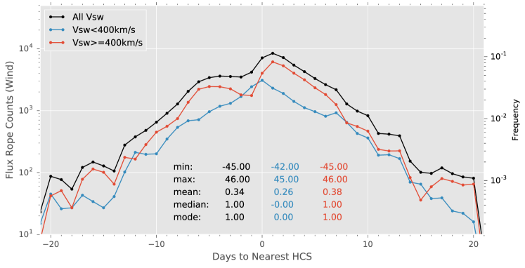
Figure 16 is the histogram of the time to the nearest HCS for the small-scale flux ropes in our database. The HCS crossing times are taken from L. Svalgaard’s list of sector boundaries in the solar wind (http://www.leif.org/research/sblist.txt). This plot indicates that the small-scale flux ropes tend to appear near the sector boundary crossings. This result is consistent with Cartwright and Moldwin’s result (see Figure 9 in Cartwright & Moldwin (2010)). However, from Figure 16 one can see that the peak of the black curve is located at 1 day after the HCS crossings, instead of 0 day given in Cartwright & Moldwin (2010). After we split the entire event set into two subsets based on solar wind speed, we find that the events with solar wind speed less than 400 km/s tend to occur within $1$ day with respect to HCS with a central peak right at $0$ day. The events with solar wind speed greater than or equal to 400 km/s tend to occur at 1 day after HCS crossing, with two broad and asymmetric peaks at $\sim-5$ days and $\sim 1$ day. Correspondingly, a broad secondary peak is also located at $-5$ days for the black curve. The similar trends of black and red curves imply that the secondary peak in black curve is contributed by the events with solar wind speed $\overline{V}_{sw}\geq$ 400 km/s. The peak at $\sim 1$ day is more pronounced, indicating a close association to HCS crossings for relatively fast solar wind. We caution not to over-interpret the peak preceding the HCS crossings, which is weak and the separation is large so that the association is much less certain. We offer an alternative explanation which is that the flux ropes near $-5$ day to HCS possibly occur right after other HCS crossings. However, these crossings are not observed due to unknown reasons. As a result, these flux ropes appear to occur at a relatively larger separation time preceding the nearest HCS as identified. This can happen when the sector boundaries are not in the ecliptic plane, so that they are not observed by spacecraft in the ecliptic plane. The blue curve ($\overline{V}_{sw}<400$ km/s) is symmetric, which is different from the red curve. The peak of the blue curve is at 0 day, indicating that the small-scale flux ropes tend to occur in the same day with HCS crossings under slow solar wind speed condition.

Figure 17: Annual small-scale flux rope counts distribution with respect to the time to the nearest heliospheric current sheet. The events are binned by 1 day. Negative days mean the occurrence time ahead of HCS crossing.

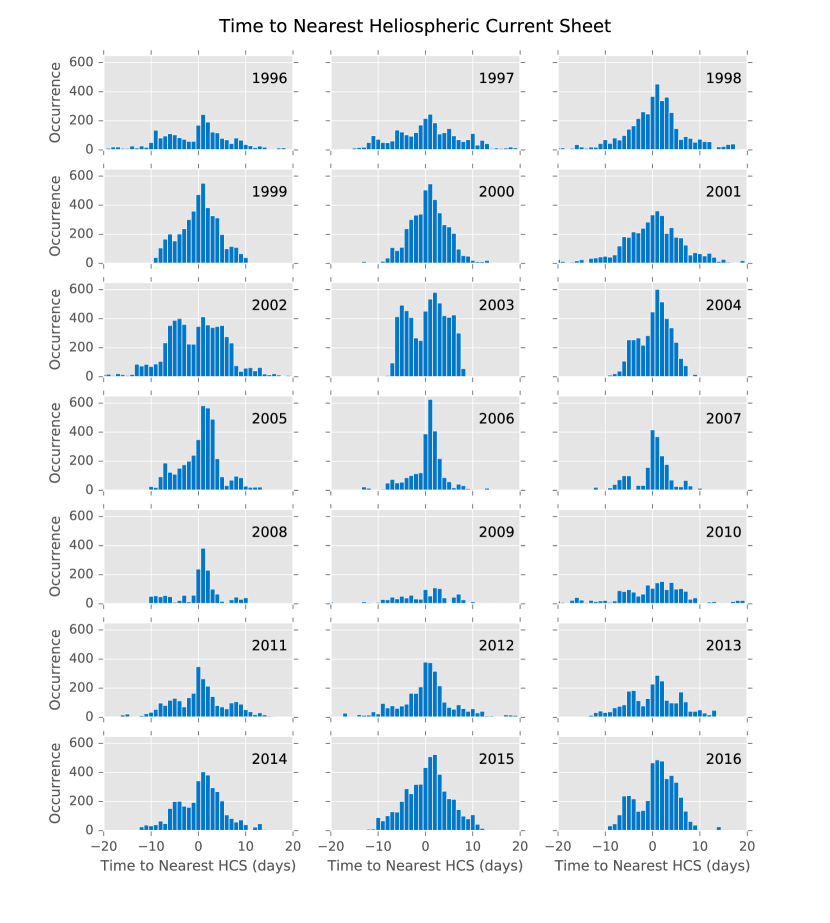
In order to look into more details on the distribution of flux rope occurrence time/location with respect to HCS, we plot the histograms of days to nearest HCS for each year in Figure 17. From Figure 17, one can see that the small-scale flux ropes do appear near HCS in each year, although the spread in time can be wide, reaching $\pm 10$ days. In addition, the distributions have year by year variations. During solar cycle 23 (1996$\sim$2008), the histograms show a triangle distribution in the years 1998, 1999, 2000, and 2001, all of which are during ascending phase of solar activity. The histograms show an additional peak near $-5$ days in the years 2002, 2003, and 2004, all of which are during descending phase. However, in solar cycle 24, there is no such a clear classification. The double peaks show up in years 2011, 2013, 2014, and 2016, in which 2011 and 2013 are during the ascending phase, while 2014 and 2016 are during the descending phase. From the analysis on Figure 16, we concluded that the secondary peaks near $-5$ day are more directly associated with medium and high speed solar wind. In Figure 17, most of those years that have secondary peaks are during the descending phase of each solar cycle, which is usually dominated by high speed solar wind streams.

Figure 18: The 2-D histograms of flux rope average proton temperature versus time to the nearest HCS. The horizontal axis is binned by 1 day. Negative values mean the time ahead of HCS. Subplots (a) to (e) are histograms under different solar wind speed conditions, and subplot (f) is the histogram for the entire event set. The color bar represents the small-scale flux rope counts.

Figure 19: The 2-D histograms of flux rope average proton number density versus time to nearest HCS. The format is the same as in Figure 18.

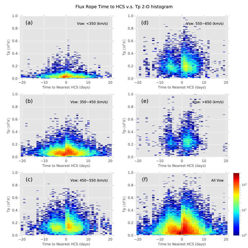
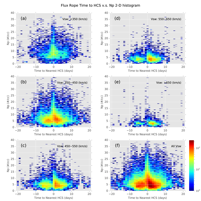
Figures 18 and 19 are the 2-D histograms of time to nearest HCS versus average proton temperature and average proton number density, respectively. Figure 18 (a) and (b) show that the small-scale flux ropes with lower proton temperature spread widely around the HCS. Figure 18 (c), (d), and (e) show that in medium and high speed solar wind, there are fewer number of small-scale flux ropes appearing far from HCS, and the proton temperature is elevated. The triangle outline in Figure 18 (f) shows a pattern consistent with Figure 16. Each panel of Figure 19 shows that the flux ropes with higher proton number density are more likely to appear near the HCS. We also note the location of the colors denoting higher occurrence rate (red and yellow color). In Figure 19 (a), the yellow color region is within the range $5\leq N_{p}\leq 15$. In Figure 19 (b), the upper boundary of the red and yellow color region is at about $N_{p}=15$, but the lower boundary exceeds beyond $N_{p}=5$. In Figure 19 (c) and (d) the red and yellow color region moves down to $0\leq N_{p}\leq 10$, and in Figure 19 (e), the red and yellow color region is below $N_{p}=5$. The different locations of the red and yellow color regions with different solar wind speed indicate that for higher solar wind speed, the flux ropes tend to have lower proton number density.

Combining Figures 18 and 19, they seem to indicate that small-scale flux ropes occurring at the HCS crossings (0 day) tend to have lower average proton temperature and higher average density, consistent with the general plasma property of the HCS, embedded in relatively low speed streams. The opposite seems to be the case for flux ropes occurring in the vicinity of HCS, within $\pm 10$ days.

7 Summary and Discussion

In summary, we have developed a new small-scale magnetic flux rope detection algorithm based on the GS equation, and applied this approach to Wind spacecraft in-situ measurements to detect small-scale magnetic flux ropes. We successfully detected 74,241 small-scale flux rope events from 1996 to 2016, covering two solar cycles. We have described, in length, the detailed automated detection algorithm and the statistical properties resulted from the detected events. This large number of small-scale flux ropes has not been discovered by any other detection approach or in any other previous studies, owing to the implementation of a highly computerized and automated algorithm rooted on the most general theoretical considerations. We build and maintain a flux rope database online to provide scientific community open access to this database. In practice, we have relied on high-performance computing facilities to fulfill this non-trivial task. By developing this database, we contribute to the study of relevant physical processes throughout the heliosphere. It is expected that the database will be expanded by including additional results from other spacecraft missions, covering a range of helio-latitudes and heliocentric distances. We hope that this database will benefit the broader scientific community of space plasma physics and astrophysical research.

Using this database, we have performed the statistical analysis as well as individual case studies on small-scale magnetic flux ropes in the solar wind, and obtained a number of significant results as summarized below:

1. The occurrence of small-scale magnetic flux ropes has strong solar cycle dependency. The occurrence count is about $3,500$ events per year on average over the past two solar cycles.

2. The small-scale magnetic flux ropes tend to align along the Parker spiral direction, in the ecliptic plane. This is consistent with the orientation pattern of “flux tubes”. This indicates that they belong to the general population of “flux tubes” identified in the same space plasma regime.

3. The small-scale magnetic flux ropes show different statistical properties under different solar wind speed conditions. In low speed ($<400$ km/s) solar wind, the flux ropes tend to have lower proton temperature, and higher proton number density, and the event counts peak at the HCS. In high speed ($\geq 400$ km/s) solar wind, they tend to have higher proton temperature and lower proton number density. The event counts peak near the vicinity of the HCS, $\sim$ 1 day later.

4. Both the duration and scale size distributions obey the power law. The power index close to -2 suggests that the larger scale size flux ropes (0.01 $\sim$ 0.05 AU) in our database under the condition of relatively high speed solar wind ($\overline{V}_{sw}\geq$400 km/s) may have closer relation to a solar source than the small-scale flux ropes under other conditions, considering the similar distributions of events with clear solar origin, i.e., flares and CMEs.

5. From the waiting time analysis, we found that the distribution for the shorter waiting time can be fitted by an exponential function, indicating that these flux ropes may undergo the pure Poisson process. The distribution associated with longer waiting time can be fitted by a power law function, indicating the clustering behavior of these flux ropes. The break point is at 60 $\sim$ 80 minutes.

6. The wall to wall time distribution obeys double power law with the break point at about 60 minutes as reported separately by Zheng & Hu (2018) which corresponds to the typical correlation length scale in solar wind turbulence (Matthaeus et al., 2005). This result is consistent with the WTDs of intermittent structures (current sheets) from MHD turbulence simulations for the inertia range that is covered by the scale size range in our database.

7. The study of the locations of small-scale magnetic flux ropes with respect to the HCS shows that the small-scale magnetic flux ropes tend to accumulate near the HCS, especially for the flux ropes under slow solar wind condition ($\overline{V}_{sw}<$400 km/s).

8. Some additional statistics show that the small-scale magnetic flux ropes with larger scale sizes tend to have low proton temperature, and tend to appear in slow speed solar wind. These behaviors, especially the former, are similar to MCs.

9. There is little cycle-to-cycle variation in the statistics of the majority of selected bulk parameters for solar cycles 23 and 24, except for the average magnetic field magnitude and plasma $\beta$. The average magnetic field magnitude within flux rope intervals is weaker in cycle 24.

We had reported in Zheng & Hu (2018) that the wall-to-wall time distribution obeys double power laws with the break point at 60 minutes (corresponding to the correlation length in solar wind turbulence), which is consistent with the waiting time distributions of intermittent structures from magnetohydrodynamic (MHD) turbulence simulations and the related observations. Through our unique approach, we provided the direct evidence in supporting the view of locally generated coherent structures intrinsic to the dynamic processes in the solar wind as manifested by magnetic reconnection and inverse turbulence cascade. We also performed case studies on the small-scale magnetic flux ropes downstream of interplanetary shocks, and found that the peaks of enhanced ions flux correspond to the merging X-line between two adjacent flux ropes, indicating that the merging flux ropes are able to energize particles within certain energy bands (Zheng et al., 2017).

These results support the notion of a “sea of flux ropes”, i.e., the ubiquitous existence of SSMFRs in the solar wind medium. They are expected to play an important role in fundamental space plasma processes. For example, a recent study by Zhao et al. (2018b) revealed detailed observational signatures of particle energization by small-scale magnetic flux ropes, which fit the theory of Zank et al. (2014, 2015); le Roux et al. (2015, 2016, 2018). Over a hundred SSMFR events were identified based on the GS reconstruction approach described here from the Ulysses spacecraft in-situ measurements over a time period of two weeks. They appear to co-locate with the energetic proton flux enhancement and the theoretic predictions fit the observed time-intensity profile and particle spectra well. It is therefore promising to further pursue more advanced study of flux rope dynamics involving contraction and merging that can be better addressed by other GS-type and full MHD-based approaches (Hasegawa, 2012; Hu, 2017).

As a point for discussion, Table 4 lists, as a first attempt, the observational evidence obtained from our analysis, in support of the two competing views on the origin of small-scale magnetic flux ropes. Each column contains the results that have been considered well established and exclusive for the corresponding origination mechanism. This is nowhere near to be final and we expect the table to be updated when further analyses are to be carried out, especially when the new discoveries are expected to be returned by the Parker Solar Probe and Solar Orbiter missions. Additionally, based on the present analysis results, the event occurrence rate, the axial orientations, and the power-law distributions in duration and scale sizes seem to be arguably supporting both hypotheses, at least not in direct contradiction to either view. For example, Borovsky (2008) analyzed the orientations of 65,860 flux tubes from 1998 to 2004 identified by searching for their boundaries, usually corresponding to discontinuities from the ACE spacecraft in-situ measurements. He found that the axial orientations are mostly aligned with the nominal Parker spiral direction at 1 AU. He therefore advocates the view that these flux tubes are distinct from one another and still rooted on the Sun. They form the “spaghetti-like” structure of the solar wind, connecting back to the source. On the other hand, such axial orientations are also consistent with the view that these structures are generated from solar wind turbulence (e.g., Matthaeus et al., 2007; Servidio et al., 2008; Zank et al., 2017) which has a prominent 2D component and the associated (perpendicular) guide field along the Parker spiral direction. Another controversial issue concerns the phenomenon of the accumulation of these small-scale magnetic flux ropes near HCS. This had long been considered as an evidence supporting the view that they originate locally across the HCS, presumably through magnetic reconnection. On the other hand, these structures may also originate from streamer belts in low corona, as shown by the latest numerical simulations of generation of “plasma blobs” (Higginson & Lynch, 2018). Therefore the HCS could serve as a conduit for them to propagate out and reach 1 AU, although detailed studies on their configurations suitable for the GS reconstruction approach may be able to discern these two possible scenarios.

Table 4: Observational evidence in support of two competing views on the origin of small-scale magnetic flux ropes.

Solar Origin	Local Origin
Flux rope configuration similar to MCs	—
—	Properties similar to 2D MHD turbulence
—	Plasma properties different from MCs
—	No significant cycle-to-cycle variations

It is worth noting that in our database there may still exist events with relatively small duration overlapping with large-scale ICMEs identified by other sources, either published or archived online. We did not take the effort in eliminating those from our current database, since the impact is minimal, especially for the small-duration events we are most interested in with duration less than 1 hour (Zheng & Hu, 2018). They occur at a rate of a few hundreds a month (see Figure 3), compared with the occurrence of ICMEs at a rate of no more than 2-3 a month, on average (Yu et al., 2016). Therefore the possible error introduced in the event count is $\lesssim$1%. Of course individual users can take the further steps of eliminating these events by cross-checking with lists of well-identified ICMEs, depending on their own needs. A remedy to this is to extend our search window sizes to include longer duration up to tens of hours. Such an effort is currently undertaken for the ACE spacecraft measurements, so that large-scale flux rope ICMEs can also be identified through our automated approach.

References

- Aschwanden & McTiernan (2010) Aschwanden, M. J., & McTiernan, J. M. 2010, The Astrophysical Journal, 717, 683. http://stacks.iop.org/0004-637X/717/i=2/a=683
- Bak et al. (1987) Bak, P., Tang, C., & Wiesenfeld, K. 1987, Phys. Rev. Lett., 59, 381. https://link.aps.org/doi/10.1103/PhysRevLett.59.381
- Borovsky (2008) Borovsky, J. E. 2008, Journal of Geophysical Research (Space Physics), 113, A08110
- Bruno et al. (2001) Bruno, R., Carbone, V., Veltri, P., Pietropaolo, E., & Bavassano, B. 2001, Planetary Space Science, 49, 1201
- Cartwright & Moldwin (2010) Cartwright, M. L., & Moldwin, M. B. 2010, Journal of Geophysical Research (Space Physics), 115, A08102, a08102. http://dx.doi.org/10.1029/2009JA014271
- Feng et al. (2007) Feng, H. Q., Wu, D. J., & Chao, J. K. 2007, Journal of Geophysical Research: Space Physics, 112, a02102. http://dx.doi.org/10.1029/2006JA011962
- Feng et al. (2008) Feng, H. Q., Wu, D. J., Lin, C. C., et al. 2008, Journal of Geophysical Research: Space Physics, 113, A12105, a12105. http://dx.doi.org/10.1029/2008JA013103
- Georgoulis & Vlahos (1998) Georgoulis, M. K., & Vlahos, L. 1998, Astronomy and Astrophysics, 336, 721
- Gopalswamy et al. (2015) Gopalswamy, N., Yashiro, S., Xie, H., Akiyama, S., & Mäkelä, P. 2015, Journal of Geophysical Research: Space Physics, 120, 9221, 2015JA021446. http://dx.doi.org/10.1002/2015JA021446
- Greco et al. (2008) Greco, A., Chuychai, P., Matthaeus, W. H., Servidio, S., & Dmitruk, P. 2008, Geophysical Research Letters, 35, doi:10.1029/2008GL035454, l19111. http://dx.doi.org/10.1029/2008GL035454
- Greco et al. (2009a) Greco, A., Matthaeus, W. H., Servidio, S., Chuychai, P., & Dmitruk, P. 2009a, The Astrophysical Journal Letters, 691, L111. http://stacks.iop.org/1538-4357/691/i=2/a=L111
- Greco et al. (2009b) Greco, A., Matthaeus, W. H., Servidio, S., & Dmitruk, P. 2009b, Phys. Rev. E, 80, 046401. https://link.aps.org/doi/10.1103/PhysRevE.80.046401
- Guidorzi et al. (2015) Guidorzi, C., Dichiara, S., Frontera, F., et al. 2015, The Astrophysical Journal, 801, 57. http://stacks.iop.org/0004-637X/801/i=1/a=57
- Hasegawa (2012) Hasegawa, H. 2012, Monographs on Environment, Earth and Planets, 1, 71
- Hau & Sonnerup (1999) Hau, L.-N., & Sonnerup, B. U. O. 1999, Journal of Geophysical Research: Space Physics, 104, 6899. http://dx.doi.org/10.1029/1999JA900002
- Higginson & Lynch (2018) Higginson, A. K., & Lynch, B. J. 2018, ApJ, 859, 6
- Hu (2017) Hu, Q. 2017, Sci. China Earth Sciences, 60, 1466
- Hu et al. (2004) Hu, Q., Smith, C. W., Ness, N. F., & Skoug, R. M. 2004, Journal of Geophysical Research: Space Physics, 109, doi:10.1029/2003JA010101, a03102. http://dx.doi.org/10.1029/2003JA010101
- Hu & Sonnerup (2000) Hu, Q., & Sonnerup, B. U. O. 2000, Geophysical Research Letters, 27, 1443. http://dx.doi.org/10.1029/1999GL010751
- Hu & Sonnerup (2001) Hu, Q., & Sonnerup, B. U. Ö. 2001, Geophysical Research Letters, 28, 467
- Hu & Sonnerup (2002) Hu, Q., & Sonnerup, B. U. O. 2002, Journal of Geophysical Research: Space Physics, 107, SSH 10. http://dx.doi.org/10.1029/2001JA000293
- Khrabrov & Sonnerup (1998) Khrabrov, A. V., & Sonnerup, B. U. Ö. 1998, ISSI Scientific Reports Series, 1, 221
- le Roux et al. (2018) le Roux, J. A., Zank, G. P., & Khabarova, O. 2018, The Astrophysical Journal, in press
- le Roux et al. (2015) le Roux, J. A., Zank, G. P., Webb, G. M., & Khabarova, O. 2015, The Astrophysical Journal, 801, 112. http://stacks.iop.org/0004-637X/801/i=2/a=112
- le Roux et al. (2016) le Roux, J. A., Zank, G. P., Webb, G. M., & Khabarova, O. V. 2016, The Astrophysical Journal, 827, 47. http://stacks.iop.org/0004-637X/827/i=1/a=47
- Lepping et al. (1995) Lepping, R. P., Acũna, M. H., Burlaga, L. F., et al. 1995, Space Sci. Rev., 71, 207
- Li et al. (2016) Li, C., Yang, J., Li, C., et al. 2016, Scientia Sinica Physica, Mechanica and Astronomica, 46, 29501. http://phys.scichina.com:8083/sciG/EN/abstract/article_519739.shtml
- Li et al. (2014) Li, C., Zhong, S. J., Wang, L., Su, W., & Fang, C. 2014, The Astrophysical Journal Letters, 792, L26. http://stacks.iop.org/2041-8205/792/i=2/a=L26
- Lu et al. (1993) Lu, E., Hamilton, R., Mctiernan, J., & Bromund, K. 1993, Astrophysical Journal, 412, 841
- Lu & Hamilton (1991) Lu, E. T., & Hamilton, R. J. 1991, The Astrophysical Journal Letters, 380, L89
- MacKinnon & MacPherson (1997) MacKinnon, A. L., & MacPherson, K. P. 1997, Astronomy and Astrophysics, 326, 1228
- Marubashi et al. (2010) Marubashi, K., Cho, K.-S., & Park, Y.-D. 2010, Twelfth International Solar Wind Conference, 1216, 240
- Matthaeus et al. (2007) Matthaeus, W. H., Bieber, J. W., Ruffolo, D., Chuychai, P., & Minnie, J. 2007, ApJ, 667, 956
- Matthaeus et al. (2005) Matthaeus, W. H., Dasso, S., Weygand, J. M., et al. 2005, Phys. Rev. Lett., 95, 231101. https://link.aps.org/doi/10.1103/PhysRevLett.95.231101
- Miao et al. (2011) Miao, B., Peng, B., & Li, G. 2011, Annales Geophysicae, 29, 237. https://www.ann-geophys.net/29/237/2011/
- Moldwin et al. (2000) Moldwin, M. B., Ford, S., Lepping, R., Slavin, J., & Szabo, A. 2000, Journal of Geophysical Research: Space Physics, 27, 57
- Moldwin et al. (1995) Moldwin, M. B., Phillips, J. L., Gosling, J. T., et al. 1995, Journal of Geophysical Research: Space Physics, 100, 19903. http://dx.doi.org/10.1029/95JA01123
- Ogilvie et al. (1995) Ogilvie, K. W., Chornay, D. J., Fritzenreiter, R. J., et al. 1995, Space Sci. Rev., 71, 55
- Paschmann & Sonnerup (2008) Paschmann, G., & Sonnerup, B. U. O. 2008, ISSI Scientific Reports Series, 8, 65
- Pearce et al. (1993) Pearce, G., Rowe, A. K., & Yeung, J. 1993, Astrophysics and Space Science, 208, 99. https://doi.org/10.1007/BF00658137
- Press et al. (2007) Press, W. H., Teukolsky, S. A., Vetterling, W. T., & Flannery, B. P. 2007, Numerical recipes : the art of scientific computing (Cambridge University Press)
- Servidio et al. (2008) Servidio, S., Matthaeus, W. H., & Dmitruk, P. 2008, Physical Review Letters, 100, 095005
- Sonnerup & Guo (1996) Sonnerup, B. U. O., & Guo, M. 1996, Geophysical Research Letters, 23, 3679. http://dx.doi.org/10.1029/96GL03573
- Sonnerup & Scheible (1998) Sonnerup, B. U. Ö., & Scheible, M. 1998, ISSI Scientific Reports Series, 1, 185
- Sotolongo-Costa et al. (2000) Sotolongo-Costa, O., Antoranz, J. C., Posadas, A., Vidal, F., & Vázquez, A. 2000, Geophysical Research Letters, 27, 1965. http://dx.doi.org/10.1029/2000GL011394
- Vlahos et al. (1995) Vlahos, L., Georgoulis, M., Kluiving, R., & Paschos, P. 1995, Astronomy and Astrophysics, 299, 897
- Wang & Dai (2013) Wang, F. Y., & Dai, Z. G. 2013, Nature Physics, 9, 465
- Wheatland (2000) Wheatland, M. S. 2000, The Astrophysical Journal Letters, 536, L109. http://stacks.iop.org/1538-4357/536/i=2/a=L109
- Wheatland et al. (1998) Wheatland, M. S., Sturrock, P. A., & McTiernan, J. M. 1998, The Astrophysical Journal, 509, 448. http://stacks.iop.org/0004-637X/509/i=1/a=448
- Yu et al. (2016) Yu, W., Farrugia, C. J., Galvin, A. B., et al. 2016, Journal of Geophysical Research (Space Physics), 121, 5005
- Yu et al. (2014) Yu, W., Farrugia, C. J., Lugaz, N., et al. 2014, J. Geophys. Res., 119, 689
- Zank et al. (2017) Zank, G. P., Adhikari, L., Hunana, P., et al. 2017, The Astrophysical Journal, 835, 147. http://stacks.iop.org/0004-637X/835/i=2/a=147
- Zank et al. (2014) Zank, G. P., le Roux, J. A., Webb, G. M., Dosch, A., & Khabarova, O. 2014, The Astrophysical Journal, 797, 28. http://stacks.iop.org/0004-637X/797/i=1/a=28
- Zank et al. (2015) Zank, G. P., Hunana, P., Mostafavi, P., et al. 2015, The Astrophysical Journal, 814, 137
- Zhao et al. (2018a) Zhao, L.-L., Adhikari, L., Zank, G. P., Hu, Q., & Feng, X. S. 2018a, ApJ, 856, 94
- Zhao et al. (2018b) Zhao, L.-L., Zank, G. P., Khabarova, O., et al. 2018b, ApJ, 864, L34
- Zheng & Hu (2018) Zheng, J., & Hu, Q. 2018, ApJ, 852, L23
- Zheng et al. (2017) Zheng, J., Hu, Q., Chen, Y., & le Roux, J. 2017, in Journal of Physics Conference Series, Vol. 900, Journal of Physics Conference Series, 012024