Sampling-based estimation of in-degree distribution
with applications to directed complex networks
Abstract.
The focus of this work is on estimation of the in-degree distribution in directed networks from sampling network nodes or edges. A number of sampling schemes are considered, including random sampling with and without replacement, and several approaches based on random walks with possible jumps. When sampling nodes, it is assumed that only the out-edges of that node are visible, that is, the in-degree of that node is not observed. The suggested estimation of the in-degree distribution is based on two approaches. The inversion approach exploits the relation between the original and sample in-degree distributions, and can estimate the bulk of the in-degree distribution, but not the tail of the distribution. The tail of the in-degree distribution is estimated through an asymptotic approach, which itself has two versions: one assuming a power-law tail and the other for a tail of general form. The two estimation approaches are examined on synthetic and real networks, with good performance results, especially striking for the asymptotic approach.
1. Introduction
Driven by the explosion of data on a host of real world networks, the last few years have seen vigorous activity from a number of communities including computer science, statistical physics and the social sciences to develop methodology to explore large scale networks as well as formulate network models to understand the emergence of various properties of real world systems such as the high degree of clustering, heavy tailed degree distribution and so on Albert and Barabási, (2002); Newman, (2018).
One particular corner of this vast field of great importance is the setting of directed networks. Real world examples include:
-
(i)
Information and social networks: Canonical examples of these objects include the internet at the webpage level with a directed edge from page to if webpage has a link to Broder et al., (2000); Brin and Page, (1998) or Twitter networks at various levels including edges from person to if person follows or Twitter event networks over a fixed duration where one follows particular hashtags and there is an edge from to if retweets in the time interval of interest Beguerisse-Díaz et al., (2014); Golder and Yardi, (2010). One need not overstate the impact of the above networks both for every day activities as well as in determining politics and world events such as the Arab Spring Khondker, (2011).
-
(ii)
Banking and financial networks: Here examples include transnational corporations with directed (weighted) edges denoting ownership fractions Vitali et al., (2011), world trade networks with a directed edge from country to indicating positivity of export flow from country to Fagiolo, (2007) or lending activity between different banks Clemente and Grassi, (2018) to measure exposure of banks to risks. A multitude of questions have been studied ranging from exploratory analysis including clustering and statistics for “global corporate control” Vitali et al., (2011) of these directed networks to quantifying risk for contagion and the cascading of losses through such interlinked systems.
-
(iii)
Citation networks: Here the data object consists of papers in a single discipline such as condensed matter physics or across multiple disciplines Redner, (2004); Vazquez, (2001). While the data can be parsed as both directed or undirected networks at various resolutions, one canonical object of interest is via a directed network where we put an edge from paper to if paper cites . Analysis range from exploration and clustering into sub-communities (see Barabási et al., (2002); Newman, (2004) and the references therein) to detecting emerging areas or understanding the evolution of these networks over time.
-
(iv)
Trophic networks in ecology: Here one is interested in feeding relationships amongst species with directed edge from to if species preys on (in many cases vertex sets can be more general than species ranging from “taxonomically related groups of species to whole kingdoms or even non-living organic matter” Pascual and Dunne, (2005)). Questions of interest include estimation of such food webs from data, stability of the resulting systems to invasion of new species or fluctuations in density of existing species, robustness including the number of secondary extinctions triggered by loss of primary species as well as classification of keystone species.
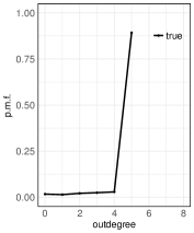
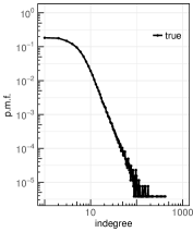
For many real directed networks, the in-degrees (i.e. the number of in-edges) of nodes and their distribution are of particular interest. To fix ideas, consider, for example, the Amazon product co-purchasing network Leskovec et al., (2007), where a directed edge from product to product indicates that after buying , a customer also would often purchase ,111There seems to be some confusion in the literature on whether to call co-purchased with , or the other way around, and we will avoid the term “co-purchased” altogether. after the latter appears in the Amazon recommendation feature “Customers Who Bought This Item Also Bought This.” The number of recommended products to purchase along with is generally small. As a result, the out-degree of a node (product) is limited (in the considered dataset, it is limited by ), and the out-degree distribution is not particularly interesting, as depicted in Figure 1(a). For this network, the in-degrees and their distribution are of greater interest. For example, the nodes with high in-degrees are the products that are also purchased when buying other products. The range and the shape of the in-degree distribution could also be of interest. The in-degree distribution for the Amazon product co-purchasing network is depicted in Figure 1(b), on the log-log scale, and the straight tail suggests, in particular, that the distribution has a power-law tail. Similar observations apply to many other directed networks, for example, citation networks that will also be considered for illustration in this work, or web link networks.
Furthermore, many real directed networks are extremely large, with large numbers of nodes and edges. Even the Amazon product co-purchasing network discussed above, which can be considered on the “smaller” side, already has 262,111 nodes and 1,234,877 edges. The Internet at the webpage level is estimated to have over 1.5 billion nodes (webpages). For such networks, it may be prohibitively expensive to gather all the information necessary to produce the in-degree distribution. To overcome this issue, sampling of nodes or edges seems to be a natural approach where the quantity of interest (the in-degree distribution in our case) would have to be inferred from the sampled data. Not surprisingly, sampling has been used extensively to deal with large networks and to infer their various quantities of interest but the in-degree distribution has received less attention yet. Some related references are discussed below, after we first describe our work in some detail.
We are thus interested in inference of the in-degree distribution through sampling network nodes and edges. Several key issues arise that we shall discuss briefly, with the goal of indicating our contributions as well:
-
•
Inherent difficulty of the problem: the latent nature of node in-degrees.
-
•
Sampling schemes to use: novel schemes based on random walks.
-
•
Inference approaches from statistical standpoint: application of penalized inversion approach and a new asymptotic approach.
An inherent difficulty in inferring the in-degree distribution is that, for example, when sampling a node, its in-degree is not observed but rather only its out-edges are seen, which contribute to the sample in-degrees of its neighbors. For example, this is very different from inferring the out-degree (or just the degree for undirected networks) distribution since the true out-degree of a sampled node is observed.
Sampling schemes to use: novel schemes based on random walks. Another feature of our problem is the potential availability of various sampling schemes to use. We shall consider below random node (vertex) and random edge sampling schemes, with and without replacement, where nodes or edges are selected uniformly at random. These sampling schemes will be abbreviated as RVS and RES, respectively. We shall also introduce several sampling schemes based on random walks, with occasional jumps to nodes or edges chosen at random from the network. When performing these random walks, the sample in-degree information will be collected either from sampling nodes or edges, and in their stationary regimes, the random walks will effectively sample nodes or edges as RVS or RES (with replacement). For one of the random walks that collects information from sampled nodes, its stationary distribution will be that of RVS by employing the standard Metropolis-Hastings technique to correct for the “bias” in its preliminary version, whose stationary distribution will have a simple and closed form. This should be contrasted to the celebrated PageRank distribution and the corresponding random walk on a network, where the walk follows one of the out-edges of a node at random or jumps to a node chosen uniformly at random from the network. The PageRank distribution does not have a simple form and the “bias” cannot be removed easily, though some attempts have been made as in [16]. Further discussion and references concerning the extensive use of random walks to sample networks can be found below. We should also note that though related, the PageRank distribution is not the in-degree distribution.
Inference approaches: application of penalized inversion approach. Turning to statistical inference, the problem of inference for the in-degree distribution from sampled data is that of statistical inversion. More specifically, if , is the in-degree distribution of a network and is its sample counterpart, we first show that
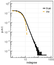
for a specified matrix which depends on the chosen sampling scheme. Part of our contributions is deriving the analytical expressions for under the considered sampling schemes. An inversion estimator of is defined as , where is a suitable inverse of and refers to the distribution of sample in-degrees. A penalized version of this “naive” estimator will also be considered, following the work of Zhang et al., (2015), in order to improve on its performance. The performance of this penalized estimator for the Amazon product co-purchasing network is illustrated in Figure 1(c), when using RVS with the node sampling probability of .
Inference approaches: a new asymptotic approach. As can be seen from the latter figure, the inversion approach does not work well in the tail of the in-degree distribution due to the inherent difficulty of the problem described above. To address estimation in the tail, we also study an asymptotic approach, assuming either an arbitrary or power-law tail of the in-degree distribution. This approach essentially involves a suitable rescaling of the sample in-degree distribution. See, for example, Figures 2–4 for illustration. The asymptotic approach for the Amazon product co-purchasing network is depicted in Figure 5. The inversion and asymptotic approaches, when combined together, can estimate the whole in-degree distribution.
Concerning related work, sampling-based estimation of degree distribution in undirected networks was considered by many researchers, for example, Stumpf and Wiuf, (2005), Leskovec and Faloutsos, (2006), Ribeiro and Towsley, (2010, 2012), Gjoka et al., (2011), Kurant et al., (2011), Lee et al., (2012), Zhang et al., (2015), to name but a few. Various sampling schemes and associated inference approaches for this task were considered, most often based on different forms of random walks. Other characteristics studied under sampling in undirected networks include global clustering coefficient (e.g. Ribeiro and Towsley, (2010)), network size (e.g. Katzir et al., (2011)), number of triangles (e.g. Wu et al., (2016)), and others.
Turning to directed networks, Henzinger et al., (2000) and Bar-Yossef and Gurevich, (2008) add reversed links when sampling a directed network through random walks to avoid being “trapped” and in this way, build over it an undirected network, which is then used to sample nodes at random. Ribeiro et al., (2012) also follow this idea by introducing a Directed Unbiased Random Walk (DURW), which combines the usual random walk on a directed network with occasional jumps. See also Murai et al., (2017). One of the random walks considered in this work is similar to DURW. Sampling algorithms in directed networks based on PageRank are studied in Leskovec and Faloutsos, (2006), Salehi and Rabiee, (2013). Out-degree distribution was among network characteristics studied under some of these sampling schemes. But as noted above, inference of the in-degree distribution has seemingly not been addressed yet (though discussed in e.g. Ribeiro et al., (2012)).
The rest of this work is organized as follows. Our sampling framework is described in Section 2. The sampling schemes based on random walks are also detailed in this section. Estimation of the in-degree distribution through statistical inversion is studied in Section 3. The section is divided into a number of parts based on the sampling scheme used. The asymptotic approach is described in Section 4. The proposed estimation methods are examined on synthetic and real networks in Section 5. Conclusions can be found in Section 6.
2. Sampling framework and sampling schemes
2.1. Directed graphs
Let be a (simple) directed graph representing the network of interest with number of vertices (nodes) and number of directed edges. We denote a generic vertex as , or or, if more than one vertex is considered, as , etc. Similarly, the notation for edges is , , , etc. The subscripts “” and “”, on the other hand, will indicate that the corresponding quantities (e.g. and ) are associated with vertices and edges, respectively. A directed edge from a vertex to a vertex will be denoted by , that is, . We shall also denote a directed edge as , to contrast it with edges in undirected graphs that will also be considered in some instances below. We assume that each vertex in has at least one (either in- or out-) edge. For notational simplicity, we shall also sometimes write (rather than ) and (rather than ).
2.2. In-degree and other quantities of interest
We focus throughout this work on the in-degree of a vertex , that is,
| (1) |
and the in-degree distribution of the graph , that is,
| (2) |
where is the number of vertices having in-degree , referred to as an in-degree count, and is the maximal in-degree in . Note that is non-zero if contains vertices with out-edges but no in-edges.
We are interested in estimating the in-degree distribution (2) through sampling. This is also equivalent to estimating the in-degree counts . We will sample either vertices or edges, which we shall refer to as sampling objects. When sampling a vertex, we assume importantly that only out-edges and out-neighbors of the vertex are “visible.” This is a common scenario encountered with real networks. The corresponding out-edges make the sampling information retained for that sampled vertex. When sampling an edge, we assume the edge to be directed and to be the sampling information retained for that sampled edge. We shall denote the (possibly repeated) sampled objects as , , further writing , for vertices and , for edges. The various sampling schemes considered in this work are discussed in Section 2.3.
For a collected sample of size , let
| (3) |
where , , refer to the sampled objects (i.e. vertices or edges), and
| (4) |
The quantities and are the sample analogues of in (1) and in (2), respectively, as suggested by the subscript “”. Note that in (4) need not be the same as and could even be larger as in sampling with replacement (discussed in this section below). The quantities ’s will be modified in Sections 3 and 4 below to yield suitable estimators ’s of ’s.
It will also be convenient to think about in and in (3) for a typical vertex , namely, a vertex chosen (uniformly) at random. Thus, we also let denote the in-degree of a vertex chosen at random. Note that
| (5) |
Additionally, let be the sample in-degree of a vertex chosen at random from the graph after sampling. We also set
| (6) |
Note that
| (7) |
Note also that we do not put a hat on and that involves normalization by (rather than, for example, by the average number of sampled vertices).
2.3. Sampling methods
We consider several sampling schemes. At the highest level, we shall distinguish between sampling with replacement (WR) and sampling without replacement (NR), the latter an acronym for “No Replacement.” In sampling without replacement, only distinct sampled objects (vertices or edges) are included in the retained information. In sampling with replacement, the same sampled objects (vertices or edges) can be included in the retained information. Samplings with and without replacement are expected to be different only when the number of sampled vertices (edges) is relatively large compared to the total number of vertices (edges). This is often the case in the setting of sampling networks where the percentage of sampled vertices (edges) have ranged in 10%-30% of the total population Zhang et al., (2015).
At the next level, we shall distinguish between objects that are sampled and through what method. We shall consider: random vertex sampling (RVS), where vertices are sampled (uniformly) at random, with or without replacement, and random edge sampling (RES), where edges are sampled (uniformly) at random, with or without replacement. We shall also sometimes write, for example, RVS-NR or RES-WR, to indicate whether NR or WR is used.
In addition, we shall also consider several random walk sampling (RWS) schemes to sample vertices or edges with replacement. These will be constructed so that in their “stationary” regimes, they will correspond to either RVS-WR or RES-WR. In this sense, RVS and RES play a central role in our analysis – the estimation methods developed for them in subsequent sections will be used with RWS as well. RWS schemes are discussed next.
2.4. Random walk samplings
We introduce below three random walk sampling (RWS) schemes: RWS1, RWS2 and RWS3. In a “stationary” regime, RWS1 will correspond to RVS-WR, and RWS2 and RWS3 to RES-WR. Before presenting their constructions and to facilitate the reading, we should also indicate several of their aspects that should not be surprising. Note that without any modification, a random walk on a directed graph might be “trapped” at a vertex without out-edges. This is often rectified by allowing the random walk to “backtrack,” that is, to walk on the directed edge backwards, thus essentially making it undirected Bar-Yossef and Gurevich, (2008). With our RWS schemes, we shall thus be building undirected graphs on top of the directed graph as the walk progresses. In addition, it is also common to introduce the possibility of jumps with RWS Murai et al., (2017). We shall allow for jumps as well and their exact role will be discussed further below. In particular, the key difference between RWS2 and RWS3 is that the walk jumps to edges in RWS2 and to vertices in RWS3.
RWS1
We construct here a RW on a suitable graph whose stationary distribution is uniform over the graph vertices, and thus corresponds to RVS-WR. Then, a sample of vertices can be selected by using such a RW and the estimation methods for RVS discussed in Sections 3 and 4 can be applied.
In addition to the directed graph , our random walk constructs and uses an undirected multigraph constructed from , which we denote by at step . The walk will also make occasional jumps to vertices chosen at random in the graph , the probability (rate) of which will be associated with a parameter . The case corresponds to no jumps, and to jumps only. The construction of the walk is summarized in the pseudo Algorithm 1. The set gathers the sampled, possibly repeated vertices and the previously visited vertices. In Step (1), the undirected graph is augmented to by including all out-edges from a vertex added to the sample . Step (2) selects a candidate vertex , which in Step (3) is either selected as the next vertex to be added in the sample or the same vertex is repeated in the sample. After the algorithm is run, the information kept consists of the out-edges seen from the vertices collected in .
-
(1)
.
-
(2)
Generate uniformly on and let be the degree of the vertex in . If , choose the potential next vertex at random from the neighbors of in . Otherwise, choose at random from the vertices of .
-
(3)
Generate uniformly on . If , update as . Otherwise, repeat as the next vertex. (If , should be read as zero.)
-
(4)
, .
-
(5)
.
A number of further comments are in place regarding Algorithm 1. We think of as an undirected multigraph which as increases, becomes the undirected multigraph constructed from by making all directed edges undirected. The selection of in Step (2) corresponds to the transition probabilities
| (8) |
when selecting for a given . The stationary distribution of these transition probabilities (in the limit of large ) is not uniform on the vertices. But it could be made uniform in a standard way through a Metropolis-Hastings (MH) algorithm as in Step (3) by noting that appearing in that step is the MH acceptance function. Indeed, this follows by noting that
| (9) |
As noted above, this argument should be viewed with on , that is, in the limit of large .
We also note that a burn-in period could be added in Algorithm 1 where the sample starts being collected only after a certain number of steps in the algorithm have been completed. The proposed random walk, without the MH correction, is also related to the DURW studied by Ribeiro et al., (2012).
Remark 2.1.
There are several reasons why jumps are used in RWS1. By varying (from corresponding to no jumps to associated with jumps only), their effect can be assessed on the performance of the estimation methods. For example, our inversion methods are quite insensitive to the proportion of jumps but the asymptotic approaches require a fairly large proportion of jumps. A related question is why not use only jumps or, equivalently, RVS, if such sampling is possible. From a practical perspective, RWs without any jumps would be preferred over RVS, since this is how real networks are typically explored. RWS schemes are thus viewed as primary approaches, which are supplemented by jumps to improve performance if needed. Another potential advantage of RWs with jumps over RVS is that jumps could be imposed only to an available subset of the graph vertices or even only to vertices from the undirected graph built from the RW.
We turn next to RWs where in a “stationary” regime, edges will be sampled at random and hence the estimation based on RES-WR can be used. We consider two RW versions, RWS2 and RWS3 below, depending on whether a jump in RW chooses an edge or a vertex at random, respectively.
RWS2
-
(1)
. Edges are added as undirected but their directionality in is kept as an attribute. Also update .
-
(2)
If , choose as or at random and set . Otherwise, set .
-
(3)
Generate uniformly on . If , set as an edge selected at random from with directionality determined by the attribute in . Otherwise, update as an edge selected at random from , and set .
-
(4)
.
-
(5)
.
A pseudo algorithm for this sampling scheme is given in Algorithm 2. We again think of as an undirected multigraph which as increases, becomes , the undirected multigraph constructed from by making all directed edges undirected. Several further comments on the loop steps of the algorithm follow. Note that gathers the collected sample of directed edges, whereas consists of previously “visited” vertices (and not edges). The variable keeps track of whether a sampled edge was selected at random through a jump (for which ) or as an out-edge from one of the vertices of the previously sampled edge (for which ). In Step (1), we emphasize that edges in are considered undirected but they are also attributed the edge direction from . We need to keep track of the direction in the collected sample since we are interested in the in-degree distribution and use the RES estimation that employs directional edges. In Step (1), the undirected graph is augmented to by adding all out-edges from the two vertices and of the directed edge added to the sample. In Step (2), if the vertex was jumped to (thus ), one of its vertices or is chosen at random as through which the RW will further explore the graph. On the other hand, if the vertex was chosen through a non-jump step of the RW (), this means that the RW previously visited the edge where , was one of the vertices – in this case, the RW will further explore the graph through the vertex .
The motivation for selecting a new directed edge into the sample in Steps (3) and (4) is as follows. For large , we can think of as the undirected multigraph , defined from as above. The graphs and have the same edges, except that in , these are made directional. The key observation then is that our algorithm samples edges at random from , and hence once attributes are added, also directed edges at random from . Indeed, to prove this key observation, it is enough to show that the stationary distribution of our RW on edges is uniform. For this, note that according to our algorithm, the transition probability for the RW on is
| (10) |
with
and
where stands for the degree of in , refers to the neighborhood of in (that is, the edges connected to ), and is also twice the number of edges in the multigraph . With some abuse of the notation and to keep notation simple, if there are two edges in between two vertices and , we denote both of these edges as . The uniform distribution on the edges is the stationary distribution for the RW since (i.e. is a doubly stochastic transition matrix). This follows from for since, for example, for ,
| (11) |
RWS3
-
(1)
. Edges are added as undirected but their directionality in is kept as an attribute.
-
(2)
.
-
(3)
Generate uniformly on and let be the degree of the vertex in . If , choose an edge at random from with directionality determined by the attribute in . Update and by . Otherwise, update by a vertex selected at random from , without updating .
-
(4)
.
We finally turn to a random walk for sampling edges where jumps will be to random vertices rather than edges. Jumping to random vertices might be preferred within the architecture of many real networks. A pseudo algorithm for RWS3 is included as Algorithm 3, and we comment on its steps and motivation next.
As in RWS2, for large , we think of as the undirected multigraph constructed from by making its directed edges undirected. Let also be the degree of a vertex in . When Algorithm 3 acts on , we shall argue that it selects the edges of at random (and hence also the edges of at random, with the directionality kept as an attribute in Algorithm 3). To make such an argument, we add an “imaginary” vertex to and connect it to each vertex of through an edge that carries a weight . Other edges in are then assumed to have weight . The resulting multigraph with the added “imaginary” vertex and edges is denoted . The edge weight, or , plays a role only when sampling randomly from a collection of edges, in which case their weights determine the sampling probabilities. For example, two edges with weights and would be sampled with the respective probabilities and .
Now, note that Step (3) of Algorithm 3 can be reformulated for by stating that an edge is selected randomly from , with the edge weights determining sampling probabilities. Indeed, for such sampling, an edge from would be selected with the probability , and the added edge to the “imaginary” vertex would be selected with the probability . In the latter case, note that the next selection would be an edge selected at random (with equal probabilities) from the “imaginary” edge back to a random vertex in . This is now captured in Step (3) of Algorithm 3 through a uniform random variable .
Let be the sample of edges collected through this reformulated Algorithm 3 acting on , that is, is the sample supplemented by the sampled edges connecting to the “imaginary” vertex. It is then enough to argue that consists of edges selected at random from since in that case, the edges of its subset would also be selected at random but now from . What needs to be shown is somewhat trivial given that edges are selected from by traveling from a vertex to one of its neighbors chosen according to a weighted degree distribution. Indeed, this simply follows by observing that such a RW on edges has its transition probabilities as
| (12) |
and one trivially has , where refers to the neighborhood of in and
to a weighted degree of .
3. Estimation by inversion
We consider inference of the in-degree distribution separately for sampling without replacement (Section 3.1) and sampling with replacement (Section 3.2). All the proposed estimators will involve a matrix inversion in one of their key construction steps, hence the reference to estimation by inversion. Inversion can and usually should also be supplemented by a suitable weighted least-squares approach with penalization, as explained in Section 3.3 below.
We shall describe the estimators in general terms first. They will involve coefficients specific to a sampling scheme. These coefficients will then be specified in Sections 3.1–3.2, for the sampling schemes listed in Section 2, that is, RVS, RES and RWS. The estimator in (4) is biased for the in-degree count , as well as in (3) for (for the latter, see also Remarks 3.2 and 3.4 below). In fact, for the considered sampling schemes, by using (7), we have that
| (13) |
and in a matrix form
| (14) |
where , and is a matrix specific to a sampling scheme, with in view of (13). The latter probability should be read as: assuming that a vertex has in-edges, what are the chances that of these in-edges will be selected through sampling?
In general, is not a square matrix. This suggests that an unbiased estimator of the in-degree counts should be defined as
| (15) |
where and is the (left) generalized inverse of , provided that has full column rank.
3.1. Sampling without replacement
The matrices for the RVS and RES schemes are specified below. The section concludes with several remarks shedding further light on the estimator (15).
RVS
For random vertex sampling without replacement, the maximum observable in-degree is and the entries of the matrix are
| (16) |
Indeed, with the interpretation of around (13)–(14), for a vertex to have in-degree after sampling, it has to have in-degree in the original graph, and then of its in-neighbors have to be sampled and vertices have to be sampled from the remaining vertices of the graph. The upper bound on is used because the maximum observed value of is the smaller of the sample size and the value of the in-degree . Also, if , at least in-degree is observed. In practice, one typically has , and therefore is a square matrix of dimension . Note also that the columns of the matrix correspond to the hypergeometric distribution with parameters , and .
RES
As above, we have and has entries
| (17) |
We note that the counts defined in (4) and entering (15) are just the in-degree counts of the sampled graph, that is, the graph obtained by connecting the graph vertices by the directed edges retained in the used sampling procedure.
Remark 3.1.
As noted above, the matrix in (16) or (17) is usually a square matrix when sampling real networks. It is then upper triangular, and so is its inverse used in the definition of the estimator (15). In particular, will be zero for those such that for . This suggests that (15) should be used with replaced by the largest in-degree obtained after sampling, which does not require the a priori knowledge of . But note that a priori knowledge (or an estimate) of and would be required to compute (16) and (17).
Remark 3.2.
It is interesting to contrast the estimators defined above to the so-called Horvitz-Thompson (HT) estimation often employed in sampling without replacement (see e.g. Thompson, (2012), Tillé, (2006)). We noted above that the estimator in (3) is biased for . In fact, an unbiased estimator is the HT estimator defined as
| (19) |
where is the probability that object (i.e. vertex or edge) is included in the sampling procedure. (As there are samples that may be chosen to include a given vertex without replacement, it follows that is the probability that the vertex is included in the sample; similarly, we have .) It then seems reasonable to set
| (20) |
as an estimator for , where denotes the “floor” integer part. But the estimator will be biased for as well. In fact, if developed, the whole inference procedure would essentially be the same as that described above in the section. Assuming , note that
that is, the vector of would consist just of the times repeated values of the vector of . One could write a formula for the vector of analogous to (14) but the corresponding probability matrix would similarly repeat the rows of the matrix . To make an inverse, the repeated rows of the probability matrix (and the corresponding repeated entries of ) would have to be removed and the resulting inversion approach would be no different from that for presented above.
3.2. Sampling with replacement
We now turn to sampling schemes with replacement. The matrices for RNS, RES and RWS are specified below.
RVS
For random vertex sampling with replacement, the maximum in-degree is and the matrix has the entries
| (21) |
Indeed, with the interpretation of around (13)–(14), note that selects of the sampled vertices that point to a vertex with in-degree , with being the probability of a sampled vertex pointing to the vertex with in-degree and being the probability of the complementary event. Note that the columns of the matrix correspond to the binomial distribution with parameters and .
RES
As above, and is a matrix with the entries
| (22) |
We note that the counts defined in (4) and entering (15) can be thought here as the in-degree counts of the sampled multigraph, that is, the multigraph obtained by connecting the graph vertices by the directed and possibly repeated edges retained in the used sampling procedure.
Remark 3.3.
In contrast to Remark 3.1, we do not have an explicit form of the inverse of the matrix (assuming it is square). Additionally, note that the choice of in (15) is somewhat arbitrary. In practice, we take to be the largest in-degree observed in the sample. We also note that a priori knowledge (or an estimate) of and would be required to compute (21) and (22).
Remark 3.4.
It is interesting to contrast the estimators defined above to the so-called Hansen-Hurwitz (HH) estimation often employed in sampling with replacement (see e.g. Tillé, (2006), Thompson, (2012)). For example, an unbiased estimator for is the HH estimator defined as
| (23) |
where to the probability of sampling at step (i.e. a vertex is sampled with probability and an edge with probability ) . One could then set
| (24) |
as an estimator for . The estimator will be biased. In fact, the whole inference procedure would essentially be the same as that described above in the section. Assuming , note that
Then, the situation is analogous to that discussed in Remark 3.2, and similar conclusions can be drawn.
Remark 3.5.
Our distinction between samplings with and without replacement might appear somewhat restrictive in the following sense. Note that a sampling procedure with replacement can be carried out (e.g. random vertex sampling with replacement) but then only distinct sampled objects be kept for inference under “sampling without replacement,” with the latter referring rather to how collected information is used. In fact, one could develop an analogous inversion approach for such sampling schemes as well, with their own probability matrices . But we found “sampling without replacement” inference for these sampling schemes to be slightly inferior to those with replacement when all sampled information collected without replacement is used. To be more specific, consider the first sample obtained through vertex sampling with replacement but where only distinct vertices are kept for inference, and the second sample where all vertices are kept for inference. For these two samples, we found inference for the second to be slightly superior. This probably should not be too surprising but might also go against some of the current practices (e.g. Zhang et al., (2015)) where inference is made on sample graph (see discussion below Eq. (22)) even if vertices/edges repeat in sampling with replacement as when using a random walk. For the above reason and for simplicity sake, we decided not to include sampling schemes with replacement where only distinct sampled objects are kept for inference.
RWS
The inversion results of this section for RVS and RES can be used in the case of RWS1 and RWS2/3, respectively, since vertices and edges are sampled uniformly at random in their “stationary” regimes.
3.3. Penalized inversion
The performance quality of the estimator (15) is rather poor in our sampling settings because the condition numbers of the matrices are generally quite large. See Section 2.1 in Zhang et al., (2015) for a related discussion. For example, the condition number of the matrix in (21) is approximately when , and (see also Section 5.2).
The quality of the estimation can be improved by considering a penalized estimation. We follow here the constrained, penalized weighted least-squares approach for this problem considered in Zhang et al., (2015), Section 3, used for undirected graphs and different sampling methods. More specifically, the penalized estimator is defined as the solution to the optimization problem
| (25) |
subject to (with )
| (26) |
In the objective function (25), is a penalty parameter (whose choice is discussed below), is the second-order differencing operator defined as in Eq. (3.2) of Zhang et al., (2015), namely,
| (27) |
and used to have smoother solutions, and is a suitable weight matrix. Following Zhang et al., (2015), we take
| (28) |
The optimization problem (25)–(26) is implemented by rewriting the objective function as a quadratic function of , and then solving it through the function solve.QP in the R package quadprog Turlach and Weingessel, (2013).
The penalty parameter is chosen based on the SURE (Stein’s unbiased risk estimation) method introduced in Eldar, (2009). The use of the SURE method in a context analogous to (25)–(26) is explained in Zhang et al., (2015), Section 3.2, which we refer the reader to for more details. We also use the same tuning parameters as discussed in Section 4.1 of Zhang et al., (2015).
4. Asymptotic approach
The estimators introduced in Section 3 perform poorly for the in-degree distribution tail (as already noted in Section 1 and can be seen from the numerical results in Section 5). Estimation in the tail could be addressed through an asymptotic approach, which can then be combined with the inversion to recover the in-degree distribution over its full range. We shall first explain the basic idea behind the asymptotic approach, and then describe two methods inspired by this approach (Section 4.1). Some of the constants in one of the methods will be specific to the sampling scheme and will be derived separately for sampling without replacement (Section 4.2) and sampling with replacement (Section 4.3).
4.1. Basic idea and methods
To explain the basic principle of the asymptotic approach, recall the two random variables and introduced in Section 2 representing the in-degree and sample in-degree of a “general” vertex, respectively. Moreover, recall the relations (5) and (7) relating these random variables to the in-degree and sample in-degree distributions. Now note that
| (29) |
where are Bernoulli random variables with parameter corresponding to the probability that one of the in-edges is sampled. For example, for RVS without replacement. Depending on the sampling scheme, the variables are independent (when sampling with replacement) or dependent (when sampling without replacement).
The relation (29) can be expressed as
| (30) |
For large and independent , the term is expected to be approximately normal and hence be negligible. A similar conclusion is also expected when are “weakly” dependent. More specifically, as long as
| (31) |
for some prescribed small level , one would in fact expect that
| (32) |
and also
| (33) |
for . In fact, under mild assumptions on and , the asymptotic relation (33) as follows from Theorem 3.2 in Robert and Segers, (2008).
The relation (33) is at the center of our asymptotic approach. It states that the distribution tail of interest (again, recall (5)) can be approximated by , which can be estimated in practice (again, recall (7)). We shall, however, also have a number of refinements of (33) that are needed for our purposes here. These have to do with:
-
1.
Working with a p.m.f. rather than a complementary CDF in (33).
-
2.
Dealing with the “flat” part of the tail of the p.m.f. of in-degrees.
-
3.
Accounting for the way the sample in-degrees are collected.
-
4.
Assuming and modeling of a power-law distribution tail.
These points are explained next.
Related to the first point above and similar to the inversion approach, we shall work with the in-degree counts and (which is equivalent to working with the in-degree distributions). The relation (33) is expected to yield or
| (34) |
An explanation and a word of caution here is that by writing (34), we treat and as “densities” so that (34) follows by differentiating both sides of (33). This “density” view will affect how the results are interpreted. More specifically, the resulting estimators of ’s should not be treated as what is expected for fixed ’s but rather as an estimated “density” for ’s from which the in-degrees of a given graph were sampled. Note also that this perspective is slightly different from that for the inversion approach where the estimator of is obtained for that fixed .
Related to the second point above, most real networks are such that a range of large in-degrees occurs in the network exactly once. That is,
| (35) |
and similalrly
| (36) |
From a modeling perspective, it is interesting to estimate and , and thus also to model the behavior (35). An assumption similar to (35) was also made in Murai et al., (2017) in the context of the degree distribution of undirected graph.
In connection to the third point above, we note that (34) cannot be expected to be used to capture (35). This has nothing to do with the way (34) was derived or its validity but rather with the way the sample in-degrees are collected. That is, note that after sampling, one would similarly have for a range of large and, rescaling these twice by as in (34) would not give (35) because also multiplies in (34). This should be contrasted with the sampling of according to (29) for independent copies of and ’s, assuming follows the distribution satisfying (35). In this case, as we checked numerically but will omit details for shortness sake, the relation (34) would also recover the behavior (35). Our asymptotic methods will need to account for these observations, by modeling (35) separately.
Finally, related to the fourth point above, some of our methods will be based on the assumption that the in-degree distribution has a power-law tail, namely,
| (37) |
where and appears in (35). We use the approximation sign “” here and below to indicate that our arguments are not completely rigorous mathematically (though that could also be formalized but at the expense of cumbersome technicalities). It is well known that the in-degree counts in many real networks follow a power-law behavior (37) (see e.g. Leskovec and Faloutsos, (2006), Gjoka et al., (2011) and Murai et al., (2017)).
We next present two methods inspired by the asymptotic approach discussed above: the ASYM method and the LINE method. The LINE method will be constructed by assuming the power-law behavior (37), whereas this assumption will not be made in the ASYM method.
ASYM method:
As discussed around (34), the asymptotic approach suggests setting
| (38) |
where is an estimator for in (36), given by
| (39) |
(if the argmin results in several ’s, the minimum of these is taken for ). In order, to account for the fact that the “flat” part of the distribution in (35) also contributes to even for up to after sampling, we shall use
| (40) |
The idea here is that through sampling, the flat “density” at value translates into another flat “density” but at value : it is this part which is subtracted from . For the “flat” part of the distribution, we shall take
| (41) |
where is the observed largest sample in-degree and is an estimator for . In view of (32), we take
| (42) |
That is, using (41) we shall just take the “flat” part of and stretch it over to . By doing so, the goal is to capture possibly any variability in the “flat” part of that would be reflected in that for .
LINE method:
At the level of CDF, the relation (33) shows that the power-law is preserved after sampling and also vice versa. To be more rigorous (since (33) does not imply an analogous result for the p.m.f.’s in general), we will show that (37) implies
| (43) |
and
| (44) |
The quantities , will depend on the sampling method used. Though note also that in view of (33), one expects
| (45) |
Consider now some estimates and modeling the in-degree counts satisfying (43)–(44), namely,
| (46) |
where is defined by (39). For example, for , one could use the maximum likelihood estimator of Clauset et al., (2009) that is part of the R package igraph Csardi and Nepusz, (2006). The relation (37) then suggests that the tail of the power-law in-degree distribution could be estimated as
| (47) |
where the use of instead of will make the results slightly more precise in practice for moderate . The estimator is defined as follows, by relating and , write
| (48) |
for a constant . Then, we expect from (37) that
| (49) |
and, hence,
| (50) |
We also need to define an estimator for the behavior (35), which we take as
| (51) |
where is defined as in (42).
Following (34), by writing (51), we actually view as a “density” for the specified values of , that is, we do not claim that for all in the range (or how many ’s are such). If needed, this “density” could be normalized to 1, when it is produced over the whole range of from 0 to .
Remark 4.1.
In view of (31), the ASYM method is expected to be particularly powerful when the largest in-degree is large. Indeed, for example, with and , note that becomes . Furthermore, we stress again that the ASYM method applies to any distribution tail, whereas the LINE method to a power-law tail only. On the other hand, the LINE method seems to work well even for smaller , whenever a power-law tail is present.
4.2. LINE method: sampling without replacement
As in Section 3.1, we consider separately the RVS and RES schemes.
RVS
We will show that
| (52) |
where , which for large and approaches as in (45). Indeed, observe from (14) and (16) that
| (53) |
By using the normal approximation to the hypergeometric distribution (Feller, (1968), p. 194, Eq. (7.5)), we have
| (54) |
where , and is the p.d.f. of the normal distribution with mean and variance . In order to proceed with the asymptotic analysis, we shall replace with the p.m.f. of the binomial distribution with parameters and (see also Remark 4.2 below). Therefore, by substituting (54) in (53) and using the binomial replacement, we have
| (55) | ||||
| (56) |
where (55) follows from and by using Stirling’s approximation. The relations (56) and (55) justifies the form of in (52) and , respectively.
Remark 4.2.
In the argument given above, we approximated a hypergeometric distribution by a normal distribution which we then replaced by a binomial distribution. In fact, by using directly another well-known binomial approximation to the hypergeometric distribution (see e.g. Feller, (1968), p. 172, Problem 35), we obtain different that perform worse in practice and the same constant .
RES
4.3. LINE method: sampling with replacement
As in Section 3.2, we consider separately the RVS, RES and RWS schemes.
RVS
We will show that is given by
| (59) |
and for large and approaches . Indeed,
| (60) | ||||
| (61) |
RES
RWS
The asymptotic results of this section for RVS and RES can be used in the case of RWS1 and RWS2/3, respectively.
5. Data study
In this section, we first present a simulation study to illustrate and to compare the performances of the estimators introduced in Sections 3 and 4, on networks simulated from random directed graph models. We then examine the proposed estimation methods on two real-world directed networks. The study of this section was performed with the help of the R package igraph Csardi and Nepusz, (2006).
5.1. Normalizations
Under RVS-WR, vertices are sampled, with each one having on average out-edges. In order to have approximately the same number of sampled edges as for RES-WR, we set . We assume that and are known or can be estimated from suitable sample quantities of the sample graph using generalizations of the Horvitz-Thompson estimator as e.g. in Kolaczyk, (2009), Chs. 5.4 and 5.5. The comparison of RVS-WR and RES-WR against RVS-NR and RES-NR could be performed using a normalization based on a budget with different costs of sampling and re-sampling a vertex (edge) but this will not be pursued here. Any differences between sampling with and without replacement should be observable when the number of sampled vertices (edges) is large compared to the total number of vertices (edges) (say, ).
For the proposed RW algorithms that sample either vertices or edges at random with replacement (in the limit), we use the same sample size normalization as in RVS-WR and RES-WR, respectively. We also equate the jump probabilities in the different random walks. For RWS2, the jump probability, , is constant and does not depend on the degree of the vertices. For RWS1 and RWS3, the jump rate can be approximated at each step of the constructed undirected graph through , where is the mean degree of the graph. Finally, we note that typical sampling proportions used in the literature vary between and .
5.2. Synthetic directed networks
We generated 30 directed scale-free networks where the in-degree and the out-degree distributions follow a power law. The expected numbers of nodes, edges, in-degree exponent and out-degree exponent, are , , and , respectively. For each directed network, we estimated the in-degree distribution in the largest component using the inversion and asymptotic approaches under sampling methods with replacement. The proportion of vertices (edges) sampled is and the jump rate for the RWS algorithms is set to 30%.
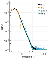
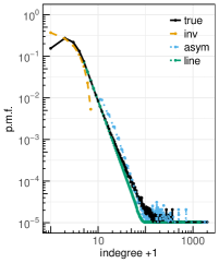
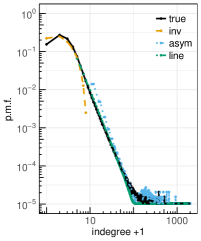
Figures 2(a)–2(b) show the estimation results for RVS-WR and RWS1, respectively, where vertices are sampled uniformly (in the limit for the RW). The “true” line corresponds to the average of the p.m.f.’s of the 30 generated networks. The average of the estimates from the inversion approach with penalization (25)–(26), labeled “inv,” can recover the beginning (bulk) of the distribution with some bias for the in-degree zero. We note that without penalization, the variance of the unbiased estimator (15) is so large that the estimator of the distribution is impractical. The penalization parameter in (25) has the effect of shrinking the estimates of the in-degree distribution, that leads to a substantial reduction in the variance, at the expense of increasing the bias. This approach also controls the variance in the tail by forcing the estimates to be equal to zero.
For the asymptotic approach, we plot in Figures 2(a)–2(b) the (average) estimates given by the ASYM method (40)–(41) and LINE method (47) (along with (59)) and (51) which allow recovering the tail of the distribution complementing the inversion approach. Since the LINE method is sensitive to the estimate of in (47), we estimate it from the “true” distribution, in order to be able to detect differences between the sampling methods (in Section 5.3 below, we use the sample in-degree distribution which satisfies (43) and is the only one available in practice). The ASYM method is accurate for larger in-degrees while the LINE method works well even for smaller in-degrees; however, the latter can only be applied to a power-law tail. The comparison between Figures 2(a) and 2(b) shows that RWS1 with a moderate jump rate can approximate RVS-WR (which can be viewed as RWS1 with jumps only).
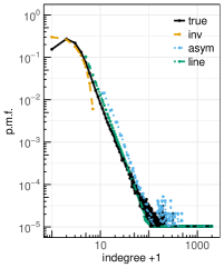
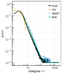
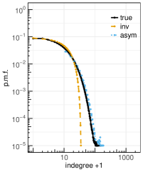
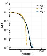
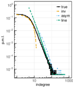
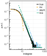
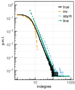
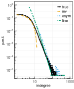
Figures 3(a)–3(c) present the (average) estimation of the in-degree distribution for RES-WR, RWS2 and RWS3, respectively, where edges are sampled uniformly (in the limit for the RWs). The inversion approach shows the same behavior as in Figure 2, with more bias for the smallest in-degrees in the case of the RWS. We note that the analysis developed in Section 4 for the LINE and ASYM methods is based on rescaling the tail of the sample in-degree distribution. For RWS1, the tail of the sample in-degree distribution tends to be smaller compared with RWS2/3 due to MH algorithm which avoids high-degree vertices; on the other hand the tail of the sample distribution tends to be smaller with RWS2 than with RWS3 because of the jumps of the former to random edges instead of vertices which somehow produce a more uniform sample (this explains the differences in Figures 2(b) , 3(b) and 3(c) for the LINE and ASYM methods). The ASYM method is accurate for large in-degree values. We also found that the estimation with the inversion approach for all sampling methods is less sensitive to changes in the jump rate than when using the asymptotic approach.
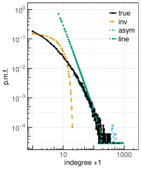
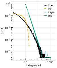
Figure 4 shows the (average) results of 30 generated random directed graphs with exponential in-degree distribution for RNS-WR and RWS1, where we decreased the sampling probability and jump rate. The number of vertices and edges generated are the same as in the power-law networks above. Only the inversion and ASYM method are used to estimate the in-degree distribution. The inversion approach shows better performance over the power-law networks above due to the form of the p.m.f. at the beginning (decreasing slowly with the in-degree). A better fit is also shown with the ASYM method for the tail. We omit the plots for RES-WR and RWS2/3 but similar conclusions can be drawn.
5.3. Real-world directed networks
We examine here the suggested estimation methods on two real directed networks. The first network is the Amazon product co-purchasing network discussed in Section 1. Figures 5(a)-5(c) depict the performance of estimation using our RWS schemes on this network with and jump rate 30%. Due to the particular form of the bulk of the in-degree distribution, the inversion method works well for the beginning of the distribution range. For the LINE method, the parameter in (47) is estimated from the sample in-degree distribution (and the same for the HEP-PH network below). The discussion concerning the power-law networks in Section 5.2 above and more specifically on the differences of the RWS schemes for the asymptotic approach applies here as well. For reference and for comparison to RWS1 in Figure 5(a), we also include in Figure 5(d) the estimation results for RWS-WR. When combined together, the inversion and asymptotic approaches approaches estimate the whole underlying in-degree distribution.
The second network is a citation network known as HEP-PH (high energy physics phenomenology) from the e-print arXiv originally described in Gehrke et al., (2003). The dataset covers all the citations in the area for a period of ten years with 34,546 papers, 421,578 edges and the mean in(out)-degree of 12.3. If a paper cites paper , the graph contains a directed edge from to . If a paper cites, or is cited by, a paper outside the dataset, the graph does not contain any information about this. Figures 6(a)–6(b) show the estimation based on RWS1 and RWS2, respectively, with and jump rate 30%. Both sampling schemes overestimate the bulk of the distribution with the inversion approach because of the seemingly fast decay of the true distribution and the small sampling probability (not to be recovered from the sample in-degree distribution which tend to be relatively large for lower in-degrees). The tail of the distribution does not follow that closely a straight line, and therefore, the LINE method only approximates the very end of the tail. On the other hand, due to the large in-degrees, the ASYM method shows a very good fit to the tail with the performance being superior for RWS1, similarly to what was observed for the synthetic and Amazon networks considered above. The plots for RVS-WR and RES-WR are omitted since they are similar to Figures 6(a) and 6(b), respectively.
6. Discussion
The estimation of the in-degree distribution of a directed network under sampling was investigated in this paper. The problem appears to have received less attention (compared with the inference of the out-degree distribution and degree distribution of undirected networks) in part due to the latent nature of node in-degrees: when a node is sampled, its in-degree is not observed but rather only its out-edges are seen, which contribute to the sample in-degrees of its neighboors. We first considered two simplest sampling schemes, random vertex sampling (RVS) and random edge sampling (RES), where vertices or edges are selected uniformly at random (with and without replacement). We then constructed three more realistic sampling schemes based on random walks with jumps which in the limit sample vertices or edges uniformly at random (with replacement). In the latter sense, RVS and RES could be viewed as constituting the basis of our analysis.
The estimation of the in-degree distribution was formulated as a linear inverse problem, that involved a matrix dependent on the sampling scheme (RVS or RES) and relating the sample in-degree distribution to the true underlying in-degree distribution of the network. Due to the inherent difficulty in observing the node in-degree, the matrices of the sampling schemes tended to be ill-conditioned for small sampling rates. To deal with ill-conditioning, a penalized weighted least-squares estimation was proposed. An asymptotic approach was also developed to estimate directly the tail of the in-degree distribution. This analysis relied on a probabilistic asymptotic equivalence between the true and sampled in-degree distribution tails. It is much less computationally intensive than using inversion. Two asymptotic methods were presented: the LINE method which assumed a power-law behavior found in many real networks, and the ASYM method which was distribution free.
Finally, our simulations on synthetic networks of different topologies and applications to real networks showed that the inversion combined with the asymptotic approach can recovered the true in-degree distribution over its full range under sampling rates in the range 15%–20%. We found that the inversion approach was less sensitive to the RW sampling scheme and jump rate used. On power-law networks, the random walk which sampled nodes uniformly (RWS1) performed better in the estimation of the tail with the asymptotic approach, where jump rates of 30% seemed to work well in practice. The jump rates could be smaller in the case of non power-law networks.
As future problems related to this work, for example, it would be interesting to adapt the suggested methodology for quantities of interest in networks other than the in-degree distribution; to get a better sense of how the suggested methodology depends on network characteristics; or to use graph sketching (a sketch is a compact representation of data) in conjunction with sampling to infer even the same in-degree distribution.
Acknowledgment
This work was initiated during a sabbatical stay of NA at the Department of Statistics and Operations Research, The University of North Carolina, Chapel Hill. NA is thankful for the hospitality and also acknowledges support by FCT grant CRM:0022222. SB was partially supported by NSF grants DMS-1613072, DMS-1606839 and ARO grant W911NF-17-1-0010. VP was partially supported by NSF grant DMS-1712966.
Appendix A Proof of the inverse matrix in Eq. (18)
We will throughout assume that the maximal in-degree , the number of samples. Further to simplify notation, we write and . Recall the expressions of the original matrix from (16) and the corresponding asserted inverse from (18). The assertion follows from the following two observations:
I. Diagonal entries of the product: For all one has .
Proof: Using the expressions for the two matrices one has
II. Off diagonal entries of the product: For all
Proof: Since the matrices are lower triangular, it is enough to show this for . Write for some . After some elementary algebraic manipulations, it can be checked that
| (64) |
where is a constant depending on and . Thus writing and , it is enough to show that for all and ,
| (65) |
Note that the expression on the left of (65) is of the form,
where
is a polynomial of degree and in particular a polynomial of degree . Standard results regarding identities of binomial coefficients Ruiz, (1996) now imply (65) and thus (64). This completes the proof.
References
- Albert and Barabási, (2002) Albert, R. and Barabási, A.-L. (2002). Statistical mechanics of complex networks. Reviews of Modern Physics, 74(1):47.
- Bar-Yossef and Gurevich, (2008) Bar-Yossef, Z. and Gurevich, M. (2008). Random sampling from a search engine’s index. Journal of the ACM, 55(5):24:1–24:74.
- Barabási et al., (2002) Barabási, A.-L., Jeong, H., Néda, Z., Ravasz, E., Schubert, A., and Vicsek, T. (2002). Evolution of the social network of scientific collaborations. Physica A: Statistical Mechanics and Its Applications, 311(3-4):590–614.
- Beguerisse-Díaz et al., (2014) Beguerisse-Díaz, M., Garduno-Hernández, G., Vangelov, B., Yaliraki, S. N., and Barahona, M. (2014). Interest communities and flow roles in directed networks: the Twitter network of the UK riots. Journal of the Royal Society Interface, 11(101):20140940.
- Brin and Page, (1998) Brin, S. and Page, L. (1998). The anatomy of a large-scale hypertextual web search engine. Computer Networks and ISDN Systems, 30(1-7):107–117.
- Broder et al., (2000) Broder, A., Kumar, R., Maghoul, F., Raghavan, P., Rajagopalan, S., Stata, R., Tomkins, A., and Wiener, J. (2000). Graph structure in the web. Computer Networks, 33(1-6):309–320.
- Clauset et al., (2009) Clauset, A., Shalizi, C. R., and Newman, M. E. J. (2009). Power-law distributions in empirical data. SIAM Review, 51(4):661–703.
- Clemente and Grassi, (2018) Clemente, G. P. and Grassi, R. (2018). Directed clustering in weighted networks: A new perspective. Chaos, Solitons & Fractals, 107:26–38.
- Csardi and Nepusz, (2006) Csardi, G. and Nepusz, T. (2006). The igraph software package for complex network research. InterJournal, Complex Systems:1695.
- Eldar, (2009) Eldar, Y. C. (2009). Generalized SURE for exponential families: Applications to regularization. IEEE Transactions on Signal Processing, 57(2):471–481.
- Fagiolo, (2007) Fagiolo, G. (2007). Clustering in complex directed networks. Physical Review E, 76(2):026107.
- Feller, (1968) Feller, W. (1968). An Introduction to Probability Theory and Its Applications. Vol. I. Third edition. John Wiley & Sons, Inc., New York-London-Sydney.
- Gehrke et al., (2003) Gehrke, J., Ginsparg, P., and Kleinberg, J. (2003). Overview of the 2003 kdd cup. ACM SIGKDD Explorations Newsletter, 5(2):149–151.
- Gjoka et al., (2011) Gjoka, M., Kurant, M., Butts, C. T., and Markopoulou, A. (2011). Practical recommendations on crawling online social networks. IEEE Journal on Selected Areas in Communications, 29(9):1872–1892.
- Golder and Yardi, (2010) Golder, S. A. and Yardi, S. (2010). Structural predictors of tie formation in Twitter: Transitivity and mutuality. In Social Computing (SocialCom), 2010 IEEE Second International Conference on, pages 88–95. IEEE.
- Henzinger et al., (2000) Henzinger, M. R., Heydon, A., Mitzenmacher, M., and Najork, M. (2000). On near-uniform url sampling. Computer Networks, 33(1-6):295–308.
- Katzir et al., (2011) Katzir, L., Liberty, E., and Somekh, O. (2011). Estimating sizes of social networks via biased sampling. In Proceedings of the 20th international conference on World wide web, pages 597–606. ACM.
- Khondker, (2011) Khondker, H. H. (2011). Role of the new media in the Arab Spring. Globalizations, 8(5):675–679.
- Kolaczyk, (2009) Kolaczyk, E. D. (2009). Statistical Analysis of Network Data. Springer-Verlag New York.
- Kurant et al., (2011) Kurant, M., Markopoulou, A., and Thiran, P. (2011). Towards unbiased BFS sampling. IEEE Journal on Selected Areas in Communications, 29(9):1799–1809.
- Lee et al., (2012) Lee, C.-H., Xu, X., and Eun, D. Y. (2012). Beyond random walk and Metropolis-Hastings samplers: why you should not backtrack for unbiased graph sampling. In ACM SIGMETRICS Performance Evaluation Review, volume 40, pages 319–330. ACM.
- Leskovec et al., (2007) Leskovec, J., Adamic, L., and Adamic, B. (2007). The dynamics of viral marketing. ACM Transactions on the Web, 1(1).
- Leskovec and Faloutsos, (2006) Leskovec, J. and Faloutsos, C. (2006). Sampling from large graphs. In Proceedings of the 12th ACM SIGKDD International Conference on Knowledge Discovery and Data Mining, KDD ’06, pages 631–636.
- Murai et al., (2017) Murai, F., Ribeiro, B. F., Towsley, D., and Wang, P. (2017). Characterizing directed and undirected networks via multidimensional walks with jumps. CoRR, abs/1703.08252.
- Newman, (2004) Newman, M. E. J. (2004). Coauthorship networks and patterns of scientific collaboration. Proceedings of the National Academy of Sciences, 101(suppl 1):5200–5205.
- Newman, (2018) Newman, M. E. J. (2018). Networks. Oxford university press.
- Pascual and Dunne, (2005) Pascual, M. and Dunne, J. A. (2005). Ecological Networks: Linking Structure to Dynamics in Food Webs. Oxford University Press.
- Redner, (2004) Redner, S. (2004). Citation statistics from more than a century of physical review. arXiv preprint physics/0407137.
- Ribeiro and Towsley, (2010) Ribeiro, B. and Towsley, D. (2010). Estimating and sampling graphs with multidimensional random walks. In Proceedings of the 10th ACM SIGCOMM conference on Internet measurement, pages 390–403. ACM.
- Ribeiro and Towsley, (2012) Ribeiro, B. and Towsley, D. (2012). On the estimation accuracy of degree distributions from graph sampling. In Decision and Control (CDC), 2012 IEEE 51st Annual Conference on, pages 5240–5247. IEEE.
- Ribeiro et al., (2012) Ribeiro, B., Wang, P., Murai, F., and Towsley, D. (2012). Sampling directed graphs with random walks. In 2012 Proceedings IEEE INFOCOM, pages 1692–1700.
- Robert and Segers, (2008) Robert, C. Y. and Segers, J. (2008). Tails of random sums of a heavy-tailed number of light-tailed terms. Insurance: Mathematics and Economics, 43(1):85–92.
- Ruiz, (1996) Ruiz, S. M. (1996). 80.52 an algebraic identity leading to Wilson’s theorem. The Mathematical Gazette, 80(489):579–582.
- Salehi and Rabiee, (2013) Salehi, M. and Rabiee, H. R. (2013). A measurement framework for directed networks. IEEE Journal on Selected Areas in Communications, 31(6):1007–1016.
- Stumpf and Wiuf, (2005) Stumpf, M. P. H. and Wiuf, C. (2005). Sampling properties of random graphs: the degree distribution. Physical Review E, 72(3):036118.
- Thompson, (2012) Thompson, S. K. (2012). Sampling. Wiley Series in Probability and Statistics. John Wiley & Sons, Inc., Hoboken, NJ, third edition.
- Tillé, (2006) Tillé, Y. (2006). Sampling algorithms. Springer Series in Statistics. Springer, New York.
- Turlach and Weingessel, (2013) Turlach, B. A. and Weingessel, A. (2013). quadprog: Functions to solve Quadratic Programming Problems. R package version 1.5-5.
- Vazquez, (2001) Vazquez, A. (2001). Statistics of citation networks. arXiv preprint cond-mat/0105031.
- Vitali et al., (2011) Vitali, S., Glattfelder, J. B., and Battiston, S. (2011). The network of global corporate control. PloS One, 6(10):e25995.
- Wu et al., (2016) Wu, B., Yi, K., and Li, Z. (2016). Counting triangles in large graphs by random sampling. IEEE Transactions on Knowledge and Data Engineering, 28(8):2013–2026.
- Zhang et al., (2015) Zhang, Y., Kolaczyk, E. D., and Spencer, B. D. (2015). Estimating network degree distributions under sampling: an inverse problem, with applications to monitoring social media networks. The Annals of Applied Statistics, 9(1):166–199.