From phase to amplitude oscillators

Abstract

We analyze an intermediate collective regime where amplitude oscillators distribute themselves along a closed, smooth, time-dependent curve $\mathcal{C}$, thereby maintaining the typical ordering of (identical) phase oscillators. This is achieved by developing a general formalism based on two partial differential equations, which describe the evolution of the probability density along $\mathcal{C}$ and of the shape of $\mathcal{C}$ itself. The formalism is specifically developed for Stuart-Landau oscillators, but it is general enough to be applied to other classes of amplitude oscillators. The main achievements consist in: (i) identification and characterization of a new transition to self-consistent partial synchrony (SCPS), which confirms the crucial role played by higher Fourier hamonics in the coupling function; (ii) an analytical treatment of SCPS, including a detailed stability analysis; (iii) the discovery of a new form of collective chaos, which can be seen as a generalization of SCPS and characterized by a multifractal probability density. Finally, we are able to describe given dynamical regimes both at the macroscopic as well as the microscopic level, thereby shedding further light on the relationship between the two different levels of description.

I Introduction

One of the peculiarities of high-dimensional complex systems is the spontaneous emergence of nontrivial dynamical regimes over multiple scales. The simultaneous presence of a macroscopic and a microscopic dynamics in mean-field models is perhaps the simplest instance of this phenomenon and, yet, it is not fully understood. It is, for instance, not clear how and to what extent the microscopic and macroscopic world are related to one another; even the minimal properties required for the emergence of a non trivial collective dynamics are unknown. This difficulty is not a surprise, as the problem is akin to the emergence of different thermodynamic phases in equilibrium statistical mechanics, with the crucial difference that there are no Boltzmann-Gibbs weights that can be invoked and, moreover, the thermodynamic phases themselves are not steady.

Generally speaking, collective regimes in mean-field models can be classified into two large families: (i) symmetry-broken phases, where the ensemble elements split in two or more groups, each characterized by its own dynamics; (ii) symmetric phases, where all oscillators behave in the same way. Clustered Golomb et al. (1992) and chimera Kuramoto and Battogtokh (2002); Abrams and Strogatz (2004) states are the two most prominent examples of the former type, while fully synchronous and splay states are the simplest examples of the latter one. In this paper we focus on the latter class and, more precisely, on the emergence of collective chaos, our goal being to shed light on the way macroscopically active degrees of freedom may spontaneously emerge in an ensemble of identical units.

It is natural to classify the different setups according to the dynamical complexity of the single oscillators, since the overall behavior should be ultimately traced back to the rules determining the evolution of the single elements. Intrinsically chaotic elements such as logistic maps sit at the top of the hierarchy. It is known since many years that collective chaos may sponentaneously emerge as a result of subtle correlations among the single dynamical units Kaneko (1990). Collective chaos can emerge also in periodic oscillators such as the Stuart-Landau model Nakagawa and Kuramoto (1993); Vincent Hakim (1992); Marie-Line Chabanol (1997), since the macroscopic mean field can trigger and maintain a microscopic chaos, thereby giving rise to a regime similar to the previous one.

By further descending the ladder of the single-unit complexity, no evidence of collective chaos has been found in mean-field models of identical phase-oscillators, but no rigorous argument excluding that this can happen is available. In fact, in all mean-field systems of identical oscillators, the probability distribution satisfies a self-consistent functional equation which, being nonlinear and infinite-dimensional can in principle give rise to a chaotic dynamics. Nevertheless, collective chaos in phase oscillators has been found only when either delayed interactions Pazó and Montbrió (2016), multiple populations Olmi et al. (2010), or heterogeneity Luccioli and Politi (2010) is included in the model. Otherwise, at most macroscopic periodic oscillations arise (the so-called self-consistent partial synchrony SCPS) van Vreeswijk (1996); Mohanty and Politi (2006); Rosenblum and Pikovsky (2007); Pikovsky and Rosenblum (2009); Politi and Rosenblum (2015); Rosenblum and Pikovsky (2015), the simplest setup for their observation being the biharmonic Kuramoto-Daido model Clusella et al. (2016). The so-called balanced regime observed in the context of neural networks is, instead, an entirely different story, since the collective dynamics is basically the result of the amplification of microscopic fluctuations E. Ullner (2018).

Altogether, new theoretical approaches are required to improve our general understanding of the collective behavior of ensembles of dynamical units. In phase oscillators characterized by strictly sinusoidal coupling-functions (Kuramoto type) the Watanabe-Strogatz theorem Watanabe and Strogatz (1993) and the Ott-Antonsen Ansatz Ott and Antonsen (2008) imply that no more than three collective degrees of freedom can emerge. What can we say in more general contexts? In this paper, we discuss an intermediate regime, where amplitude oscillators (characterized by at least two variables) retain a key property of phase oscillators, i.e. they can be parametrized by a single phase-like variable. In practice, the amplitude dynamics is sufficiently stable to force the oscillators towards a smooth closed curve $\mathcal{C}$ such as in standard phase oscillators, but not stable enough to prevent fluctuations of the curve itself, which therefore acts as an additional source of complexity. We refer to this regime, which has been so far basically overlooked, as to Quasi Phase Oscillators (QPO). We are only aware of a preliminary study carried out by Kuramoto & Nakagawa, who performed microscopic simulations of an ensemble of Stuart-Landau oscillators Nakagawa and Kuramoto (1995). Here we develop a general formalism, which allows describing QPO at a macroscopic level. As a result, we are able to identify and describe a series of dynamical regimes ranging from plain SCPS to a new type of collective chaos. SCPS itself is already an intriguing regime. In fact, under the action of a self-consistent mean field, the single oscillators exhibit generically a quasiperiodic behavior without phase locking (no Arnold tongues). Said differently, the transversal Lyapunov exponent of each single oscillator (conditioned to a given “external” forcing) is consistently equal to zero, when a control parameter is varied. The hallmark of QPO is that the transverse Lyapunov exponent is not positive, even when the “external” mean-field forcing is chaotic: actually, it is even slightly negative, implying that the phase probability distribution is not smooth but multifractal. This is at variance with the “standard” collective chaos observed in a different parameter region of the Stuart-Landau model Nakagawa and Kuramoto (1993); Takeuchi and Chaté (2013); Vincent Hakim (1992); Marie-Line Chabanol (1997), characterized by a positive transversal Lyapunov exponent.

In Section II we introduce the model and develop the formalism, which consists in the derivation of two partial differential equations (PDEs), one describing the probability density of the oscillators along the curve $\mathcal{C}$ and the other describing the shape of the curve itself. These equations are thereby simulated to identify the different regimes: the agreement with the integration of the microscopic equations validates the whole approach. Next, an exact stability analysis of the splay state is performed in Section III, which allows determining the critical value of the coupling strength where SCPS is born. Section IV is devoted to the analysis of SCPS, leading to an exact solution for the distribution of phases and for the shape of $\mathcal{C}$. Therein we analyse also the transition to SCPS, uncovering very subtle properties: superficially, the transition corresponds to the critical point of the Kuramoto-Sakaguchi model Sakaguchi and Kuramoto (1986), which separates the stability of the splay state from that of the synchronous solution. However, this is not entirely correct, as it is known that the Kuramoto-Sakaguchi model cannot support SCPS. In fact, it turns out that the mutual coupling and, in particular, the fluctuations of the curve $\mathcal{C}$, give birth to higher Fourier harmonics, which are essential for the stabilization of SCPS. In the following section V, we analyse the increasingly complex regimes generated when the coupling is further increased. In particular, we see that the transition to chaos is rather anomalous: a sort of intermediate scenario between the standard low-dimensional route to chaos where a single exponent becomes positive, and high-dimensional transitions when the number of unstable directions is proportional to the system size. In the present context, we have evidence of the simultaneous appearance of three positive exponents, irrespective of the number of oscillators. An additional unusual feature of the chaotic dynamics is the presence of (infinitely many) nearly zero exponents, which, according to the Kaplan-York formula, make the system high dimensional in spite of the finite (and small) number of unstable directions. In section V we discuss also macroscopic and microscopic Lyapunov exponents, showing that they are consistent with one another. This equivalence is far from trivial, since in all previous instances of collective chaos the correspondence between the two spectra was at most restricted to very few exponents, the reason for the difference being that while the microscopic exponents refer to perturbations of single trajectories, the macroscopic ones refer to perturbations of the distributions of phases. Finally, section VI contains a summary of the main results and of the open problems.

II The model

Following Ref. Nakagawa and Kuramoto (1993), we consider an ensemble of $N$ coupled Stuart-Landau oscillators

$$\dot{z}_{j}=K(1+ic_{1})(\overline{z}-z_{j})+z_{j}-(1+ic_{2})|z_{j}|^{2}z_{j}$$ (1)

where $z\in\mathbb{C}$ and

$$\bar{z}=\frac{1}{N}\sum_{m=1}^{N}z_{m}$$

is the mean field. The formulation of Refs. Marie-Line Chabanol (1997); Vincent Hakim (1992) is recovered by setting $t\to Kt$, $\alpha=c_{2}$, $\eta=c_{1}$ and $\mu=K^{-1}$.

A homogeneous system of globally coupled oscillators such as (1) can display two types of stationary solutions: a state of full synchrony and incoherent states. In the state of full synchrony all the oscillators evolve periodically as $z_{j}=\overline{z}=\mathrm{e}^{ic_{2}t}$. Incoherent states correspond to a distribution of oscillators such that the mean field $\overline{z}$ vanishes. There are infinitely many ways of realizing an incoherent state, the simplest being a completely homogeneous distribution of the phases along a circle (of radius $\sqrt{1-K}$) also known as splay state.

For small coupling strength $K\ll 1$, the model can be mapped onto a Kuramoto-Sakaguchi model Rosenblum and Pikovsky (2015), which is known to give rise only to either fully synchronous or splay states. For larger coupling strength, the model displays a rich variety of dynamics, including clustered states, chimera states, and different forms of collective chaos Nakagawa and Kuramoto (1993, 1995); Marie-Line Chabanol (1997); Vincent Hakim (1992); Sethia and Sen (2014). In particular, Nakagawa & Kuramoto Nakagawa and Kuramoto (1995) reported numerical evidence of a dynamical regime where the oscillators seem to be distributed along a smooth time-dependent closed curve. In this paper, we revisit such a behavior, developing a formalism, which can, in principle, be applied to generic ensembles of mean-field driven amplitude oscillators.

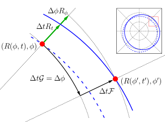
Figure 1: Schematic representation of the phase parametrization of $\mathcal{C}$ and its time evolution. Dashed blue curve depicts the shape of of $\mathcal{C}$ at time $t$, whereas the continuous blue line indicates the position of $\mathcal{C}$ at time $t^{\prime}=t+\Delta t$. The inset shows a zoom out version, with the red rectangle indicating the zone depicted in the main figure.

A general macroscopic formulation of system (1) requires the knowledge of the probability density on the complex plane $Q=Q(z,t)$. Nevertheless, if the amplitude dynamics is sufficiently stable, the oscillator variables naturally converge and are eventually confined to a closed curve $\mathcal{C}$. Whenever this is the case, $\mathcal{C}$ can be uniquely parametrized in polar coordinates by expressing the radius $R(\phi,t)$ as a function of the phase $\phi$. Accordingly we can assume that the probability density is confined to $\mathcal{C}$ so that

$$Q(z,t)=Q(z,t)\delta(|z|-R(\phi,t))=:P(\phi,t).$$

The meaningfulness of this approach is verified a posteriori by the consistency of the theoretical predictions and by the agreement with direct numerical simulations.

Our first goal is to derive the evolution equations for $R$ and $P$. In order to do so, it is convenient to express Eq. (1) in polar coordinates, $z=r\operatorname{\rm e}^{i\phi}$,

$$\dot{r}_{j} =\mathcal{F}[r_{j},\phi_{j},\overline{z}]$$

$$\dot{\phi}_{j} =\mathcal{G}[r_{j},\phi_{j},\overline{z}]\;,$$

where

$$\mathcal{F}[r,\phi,\overline{z}] =(1-K-r^{2})r+K\operatorname{Re}[(1+ic_{1})\overline{z}\operatorname{\rm e}^{-i\phi}]$$

$$\mathcal{G}[r,\phi,\overline{z}] =-c_{1}K-c_{2}r^{2}+\frac{K}{r}\operatorname{Im}[(1+ic_{1})\overline{z}\operatorname{\rm e}^{-i\phi}]\;.$$

Let us now consider a time interval $\Delta t\ll 1$ and $t^{\prime}=t+\Delta t$. At time $t$ the oscillator with index $j$ has polar coordinates $[r_{j}(t),\phi_{j}(t)]=[R(\phi,t),\phi]$ while at time $t^{\prime}$ has $[r_{j}(t^{\prime}),\phi_{j}(t^{\prime})]=[R(\phi^{\prime},t^{\prime}),\phi^{\prime}]$, as indicated in figure 1. If $R$ is smooth we have that

$$\begin{cases}R(\phi^{\prime},t^{\prime})=R(\phi,t)+\Delta t\;\mathcal{F}[R(\phi,t),\phi,\overline{z}]\\ \phi^{\prime}=\phi+\Delta t\;\mathcal{G}[R(\phi,t),\phi,\overline{z}].\end{cases}$$

Then one can write

$$\frac{R(\phi,t^{\prime})-R(\phi,t)}{\Delta t}=\frac{R(\phi^{\prime},t^{\prime})-R(\phi,t)}{\Delta t}-\frac{\phi^{\prime}-\phi}{\Delta t}R_{\phi}$$

so that

$$\frac{\partial R}{\partial t}(\phi,t)=\mathcal{F}[R,\phi,\overline{z}]-\mathcal{G}[R,\phi,\overline{z}]R_{\phi}\;.$$ (2)

On the other hand, the evolution of $P$ is determined by the angular flux at $r=R(\phi,t)$,

$$\frac{\partial P}{\partial t}(\phi,t) =-\frac{\partial}{\partial\phi}\Bigl{\{}P(\phi,t)\mathcal{G}[R,\phi,\overline{z}]\Bigr{\}}.$$ (3)

while the mean field is finally defined as

$$\overline{z}(t)=\int_{0}^{2\pi}P(\phi,t)R(\phi,t)e^{i\phi}d\phi.$$ (4)

From the expression for $\mathcal{G}[R,\phi,\overline{z}]$, one can recognize the Kuramoto-Sakaguchi structure Sakaguchi and Kuramoto (1986) of the velocity field, with however, the important difference of the additional factor $R(\phi,t)$ in the definition of the order parameter. We will see that the time dependence of $R(\phi,t)$ (it obeys a distinct differential equation) enriches the complexity of the collective dynamics.

Overall, equations (2,3,4) represent a system of two nonlinear Partial Differential Equations (PDEs) describing the macroscopic behavior of the oscillators whenever they are spread along a closed phase-parameterized smooth curve.

Such a system can be solved numerically by means of a split-step Fourier or pseudospectral method Canuto et al. (2006). The algorithm consists in expanding $R$ and $P$ spatially in Fourier space,

$$P(\phi,t) =\frac{1}{2\pi}\sum_{k=-\infty}^{\infty}\tilde{P}(k,t)e^{-ik\phi}\quad\text{and}$$

$$R(\phi,t) =\frac{1}{2\pi}\sum_{k=-\infty}^{\infty}\tilde{R}(k,t)e^{-ik\phi}$$

where

$$\quad\tilde{P}(k,t) =\int_{0}^{2\pi}d\phi\;P(\phi,t)e^{ik\phi}\quad\text{and}$$

$$\quad\tilde{R}(k,t) =\int_{0}^{2\pi}d\phi\;R(\phi,t)e^{ik\phi}.$$

By truncating the Fourier series for a large enough wavelength $M$, one can then integrate in time the different Fourier modes $\tilde{P}(k,t)$ and $\tilde{R}(k,t)$ using a standard method for ordinary differential equations. Since the computation of a nonlinear term of order $q$ in Fourier space requires $\mathcal{O}(M^{q})$ operations, it is more convenient to compute the velocity fields in real space instead. In fact, by invoking fast Fourier transform (FFT) algorithms, the computational cost of the nonlinear fluxes reduces to $\mathcal{O}(4n\log(2n))$, where $n$ is the number of points of the real support. We use a fourth-order Runge-Kutta integration method with time step $\delta t$, set to $10^{-3}$ in most of the simulations. In order to avoid aliasing errors in the successive calls of the FFT we use the 3/2-truncation rule using a real spatial grid of $n=2048$ points and a truncation of $M=680$ in the Fourier expansion. Nevertheless, in the presence of chaotic dynamics (see below) the numerics become more challenging and it is necessary to increase both spatial and temporal resolutions. Therefore, for $K>0.416$ we use $M=1024$ and $\delta t=0.5\cdot 10^{-3}$, and keep $n=2048$. In this case it is necessary to introduce a smoothing technique to prevent the growth of the aliasing errors. Thus we add a small diffusive term in equation (3),

$$\frac{\partial P}{\partial t}(\phi,t) =-\frac{\partial}{\partial\phi}\Bigl{\{}P(\phi,t)\mathcal{G}[R,\phi,\overline{z}]\Bigr{\}}+D\frac{\partial^{2}}{\partial\phi^{2}}P(\phi,t)\;.$$

A diffusion level of $D=10^{-8}$ is enough to stabilize the algorithm while preserving the dynamical properties of the system.

In order to double check our numerics we have fixed two parameters as in Ref. Nakagawa and Kuramoto (1995) ($c_{1}=-2$ and $c_{2}=3$) and treated the coupling strength $K$ as the leading control parameter. The results of our numerical simulations are reported in figures 2, 3 and 4. In figure 2 we show the time-average of the mean-field $|\overline{z}|$ computed both using the microscopic formulation of the system (1) with $N=4096$ (black plusses) and using the macroscopic equations solved with the pseudospectral method (red circles). The nice agreement confirms the correctness of the macroscopic equations.

The behavior of the order parameter unveils a series of bifurcations across various dynamical regimes, marked with vertical dashed black lines. In figure 3 we show the time evolution of the order parameter modulus $|\overline{z}|$ for different values of $K$, each belonging to a different dynamical regime. In the top panels of figure 4 we plot snapshots of $R$ (black dashed lines) and the corresponding probability densities $P$ (red lines). While the shape of the curve $\mathcal{C}$ remains very smooth when the coupling is increased, the probability profiles become increasingly rugged, revealing an increasing contribution of higher Fourier modes. This is better appreciated by looking at the bottom panels of Fig. 4, where the corresponding Power Spectral Density (PSD) is reported in a logarithmic scale (same color code for the different curves).

For $K<K_{1}\approx 0.4123$, the oscillators are uniformly distributed on a perfect circle and the mean-field $\overline{z}$ vanishes, i.e., the system is in a splay state. For $K=K_{1}$ there is a first transition to a regime where the mean-field dynamics is a pure periodic rotation on a one-dimensional torus (T1), accompanied by a quasiperiodic dynamics of the single oscillators. This regime is therefore an example of self-consistent partial synchrony (SCPS) first uncovered in a model of leaky integrate-and-fire neurons van Vreeswijk (1996) and fully described in biharmonic Kuramoto-Daido oscillators Clusella et al. (2016). In this regime, the mean-field modulus is constant (see red line in Fig. 3). In fact, both $P$ and $R$ are spatially nonuniform steady functions if observed in a suitably rotating frame (see Fig. 4(a), where we can also notice that the shape is dominated by a few long wavelength modes - panel (e)). At $K=K_{2}\simeq 0.4138$ a macroscopic Hopf bifurcation occurs, which introduces a second frequency. As a result, the collective dynamics is quasiperiodic (T2, but periodic, if observed in a suitably rotating frame) (see the blue line in Fig. 3). Now the shape of $P$ and $R$ fluctuate in time and more Fourier modes contribute (see figures 4(b) and (f)).

At $K=K_{3}\simeq 0.41588$, yet another frequency adds to the macroscopic dynamics, although indistinguishable from the average value of the order parameter. Thus, as better argued in the following, the dynamics of the order parameter becomes three-dimensional (T3) (see the green line in Fig. 3). The shape of $P$ becomes more uneven, with several bumps that evolve on time, and the spatial spectra involve higher Fourier modes (see Fig. 4(c) and (g)).

The T3 regime is stable for a small range of the parameter value; beyond $K=K_{4}\simeq 0.41605$ the system becomes chaotic. Although $R$ keeps being quite smooth, the shape of $P$ occasionally develops several peaks that become sharper upon increasing the coupling strength (see Fig. 4(d) and (h)). Such peaks generate spurious ringing artifacts that eventually lead to numerical instabilities. Nevertheless, as explained before, increasing the numerical resolution and introducing a negligible diffusion, one can accurately integrate the macroscopic equations for long times.

For yet larger $K$ values, the order parameter vanishes after a long chaotic transient. However, the asymptotic regime is not a splay state: only the first Fourier mode vanishes, while the others have non zero amplitude. In other words the distribution of angles is non uniform. The disagreement between microscopic and macroscopic simulations on the bifurcation point $K_{5}$ in figure 2 is due to the fact that macroscopic simulations cannot be run long enough for the chaotic transient to finish. Finally, if the coupling is increased even further, one ends up in the highly irregular chaotic regime studied in Nakagawa and Kuramoto (1993); Takeuchi and Chaté (2013), where the macroscopic equations (2) and (3) are no longer valid, since the oscillators are not distributed along a smooth closed curve.

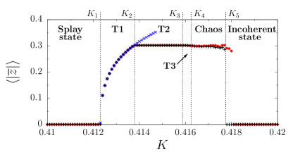
Figure 2: Time-averaged mean-field $\langle|\overline{z}|\rangle$ for different values of the coupling strength $K$ and fixed $c_{1}=-2$ and $c_{2}=3$. Black plusses show the results from microscopic simulations of the system as given by (1) with $N=4096$ oscillators computed over $10^{6}$ time units after discarding another $10^{6}$ of transient. Red circles correspond to the numerical integration of Eqs. (2) and (3) with a pseudospectral method for $10^{5}$ time units, from which $5\cdot 10^{4}$ are transient. Both microscopic and macroscopic simulations use initial conditions close to splay state. Blue crosses correspond to the semi-analytical fixed point given by Eqs. (9) and (10). Black vertical dashed lines indicate the bifurcation points between the different dynamical regimes.

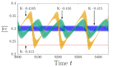
Figure 3: Time series of $|\overline{z}|$ from the numerical integration of the macroscopic equations of the system for $K=0.413$ (red), $0.415$ (blue), $0.416$ (green), and $0.4165$ (amber).

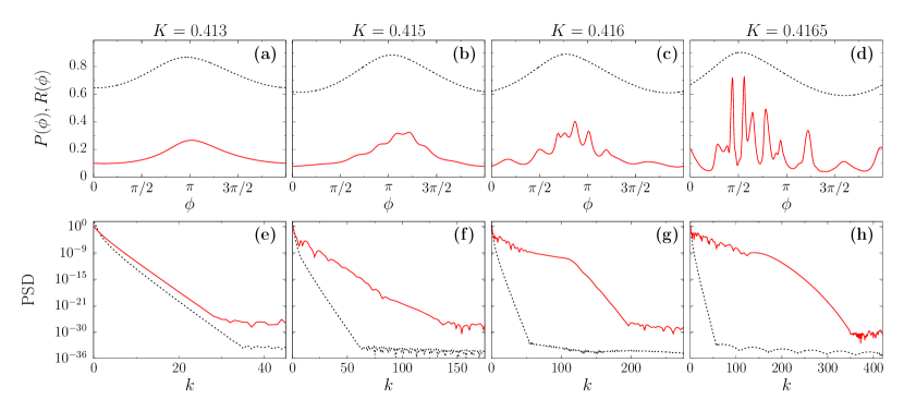
Figure 4: Snapshots of the shape of $R$ (dashed black curve) and $P$ (red continuous curve) in real space (top figures), and the corresponding Power Spectral Density in logarithmic scale (bottom figures). (a) and (e) correspond to $K=0.413$, (b) and (f) to $K=0.415$, (c) and (g) to $K=0.416$, and (d) and (h) to $K=0.4165$. Results obtained upon integrating the macroscopic equations using a pseudospectral method.

III Stability of Splay State

The macroscopic equations can be used to perform the stability analysis of the splay state by introducing the fields $u(\phi,t)$ and $v(\phi,t)$ which denote infinitesimal perturbations of the probability $P_{0}=1/(2\pi)$ and of the radius $R_{0}=\sqrt{1-K}$, respectively. Upon linearizing Eqs. (2) and  (3), it is found that

$$v_{t}=-2(1-K)v+Av_{\phi}+K\operatorname{Re}[(1+ic_{1})\overline{w}\mathrm{e}^{-i\phi}]\;,$$

and

$$u_{t}= Au_{\phi}+\frac{c_{2}\sqrt{1-K}}{\pi}v_{\phi}+\frac{K\operatorname{Re}[(1+ic_{1})\overline{w}\mathrm{e}^{-i\phi}]}{2\pi\sqrt{1-K}}\;,$$

where

$$A= c_{1}K+c_{2}(1-K)$$

and

$$\overline{w}:= \sqrt{1-K}\int_{0}^{2\pi}\!\!\!d\phi\;u(\phi,t)\operatorname{\rm e}^{i\phi}+\frac{1}{2\pi}\int_{0}^{2\pi}\!\!\!d\phi\;v(\phi,t)\operatorname{\rm e}^{i\phi}$$

is the (linear) variation of the mean-field. It is composed of two terms: the former one is the standard Kuramoto-type order parameter, while the latter accounts for fluctuations of the curve $\mathcal{C}$.

The linearized equations can be easily solved in Fourier space, i.e., by introducing

$$\tilde{v}(k,t) =\int_{0}^{2\pi}d\phi v(\phi,t)\operatorname{\rm e}^{ik\phi}\qquad\text{and}$$

$$\tilde{u}(k,t) =\int_{0}^{2\pi}d\phi u(\phi,t)\operatorname{\rm e}^{ik\phi}\;,$$

(and the corresponding inverse transforms), since they become block diagonal.

For $k\neq\pm 1$ (including $k=0$),

$$[\tilde{v}(k)]_{t} =\left[-2(1-K)-ikA\right]\tilde{v}(k)\quad\text{and}$$

$$[\tilde{u}(k)]_{t} =-ik\frac{c_{2}\sqrt{1-K}}{\pi}\tilde{v}(k)-ikA\tilde{u}(k)\;$$

so that, the evolution of $\tilde{v}(k)$ is closed onto itself and acts as an external forcing for the dynamics of the probability density, yielding the eigenvalues

$$\lambda^{(v)}_{k} =-2(1-K)-ik(Kc_{1}+c_{2}(1-K))\quad\text{and}$$

$$\lambda^{(u)}_{k} =-ik\left(Kc_{1}+c_{2}(1-K)\right)\;.$$

Altogether, the eigenvalues are arranged into two branches: the former corresponds to stable directions associated to the $\mathcal{C}$-dynamics; the latter corresponds to marginally stable directions associated to the density dynamics (this includes the zero mode, whose marginal stability is nothing but a manifestation of probability conservation). Overall the stability of the angle distribution is reminiscent of the marginal stability of the Kuramoto model.

The only exception is the first Fourier mode of $v(\phi,t)$, that is coupled back to the shape of the curve. For $k=1$ we obtain

$$[\tilde{v}(1)]_{t} =M_{vv}\tilde{v}(1)+M_{vu}\tilde{u}(1)$$ (5)

$$[\tilde{u}(1)]_{t} =M_{uv}\tilde{v}(1)+M_{uu}\tilde{u}(1)$$

where

$$M_{vv}= -2+\frac{5}{2}K-i\left(A-\frac{Kc_{1}}{2}\right)$$

$$M_{vu}= -\pi K\sqrt{1-K}(1+ic_{1})$$

$$M_{uv}= \frac{K}{4\pi\sqrt{1-K}}-i\left(\frac{c_{2}\sqrt{1-K}}{\pi}-\frac{Kc_{1}}{4\pi\sqrt{1-K}}\right)$$

$$M_{uu}= \frac{K}{2}-i\left(A-\frac{Kc_{1}}{2}\right)\;.$$

Finally, the equations for $k=-1$ are obtained by simply taking the complex conjugate of the above expressions.

Accordingly, instabilities can and actually do arise within the four-dimensional subspace spanned by the real and imaginary parts of the first modes $\tilde{v}(1)$ and $\tilde{u}(1)$. In practice one needs to determine the stability of the two dimensional complex system (5). Using the Routh–Hurwitz criterion one finds two stability conditions

$$3K<2\;,\qquad\text{and}$$

$$(2c_{1}^{2}+8c_{1}c_{2}-c_{2}^{2}+9)K^{2}-$$

$$(c_{1}^{2}+12c_{1}c_{2}-c_{2}^{2}+12)K+4+4c_{1}c_{2}<0$$

In the parameter region considered in this paper, the second inequality reveals a loss of stability for $K>K_{1}=(65-\sqrt{1025})/80=0.412304\ldots$, which corresponds to a pair of complex conjugate eigenvalues crossing the imaginary axis, i.e., a Hopf bifurcation. This bifurcation gives rise to SCPS, a periodic collective dynamics, analyzed in the following section.

IV Self-consistent partial synchrony

Above $K_{1}$, SCPS is stable within the region T1. Our general formalism, based on Eqs. (2,3,4), allows performing an analytical study of this regime.

Self-consistent partial synchrony is characterized by a non-uniform probability density, rotating with a collective frequency $\omega$, which differs from the average frequency of the single oscillators. In models where the interactions depend only of phase differences like the present one, $\omega$ is constant as well as the amplitude $|\overline{z}|$ of the order parameter. In other words, SCPS corresponds to a fixed point of Eqs. (2,3) in the moving frame $\theta=\phi-\omega t$. Since we are free to choose the origin of the phases, we select a frame where $\overline{z}$ is real and positive, i.e., its phase vanishes (so that from now on we can avoid the use of the absolute value). The equations resulting from this change of variables are

$$R_{t}=\mathcal{F}[R,\theta,\overline{z}]+\left\{\omega-\mathcal{G}[R,\theta,\overline{z}]\right\}R_{\theta}$$ (6)

and

$$P_{t}=\frac{\partial}{\partial\theta}\Bigl{(}P(\theta,t)\bigl{\{}\omega-\mathcal{G}[R,\theta,\overline{z}]\bigr{\}}\Bigr{)}.$$ (7)

accompanied by the self-consistent condition

$$\int_{0}^{2\pi}\!\!\!d\theta\;P(\theta,t)R(\theta,t)e^{i\theta}=:\overline{z}\;.$$ (8)

By imposing the time derivative of $R$ equal to zero in equation  (6), we find that the stationary shape of the limit cycle, $R_{0}(\theta)$, can be obtained by integrating the following ODE,

$$[R_{0}(\theta)]_{\theta}=-\frac{\mathcal{F}[R_{0},\theta,\overline{z}]}{\omega-\mathcal{G}[R_{0},\theta,\overline{z}]}.$$ (9)

Once a (numerical) expression for $R_{0}$ has been obtained, it can be replaced in the equation for $P$. The stationary solution $P_{0}$ can be thereby obtained by setting the argument of the $\theta$ derivative equal to a new unknown constant: minus the probability flux $\eta$. The solution reads

$$P_{0}(\theta)=-\frac{\eta}{\omega-\mathcal{G}[R_{0},\theta,\overline{z}]}\;,$$ (10)

where $\eta$ can be obtained from the normalization condition of the probability density $\int_{0}^{2\pi}P_{0}=1$. A complete expression for $R_{0}(\theta)$, and $P_{0}(\theta)$ is finally obtained by determining the two remaining unknowns, $\overline{z}$ and $\omega$, from the complex self-consistent condition (8). The resulting shapes are reported in Figs. 5(a,b) for two different coupling strengths. As expected, both $R_{0}$ and $P_{0}$ become increasingly nonuniform upon increasing the coupling strength. Blue crosses in figure 2 indicate the values of $|\overline{z}|$ obtained from this approach.

In the rotating frame, where the curve $R(\theta)$ does not depend on time, one can view the term in curly brackets in Eq. (7) as the force field acting on an oscillator of phase $\theta$, so that $\mathcal{G}(R(\theta),\theta)$ plays the role of the standard coupling term in ensembles of phase oscillators. The Kuramoto-Sakaguchi model is the simplest setup where the coupling is purely sinusoidal, i.e., $\mathcal{G}=G\sin(\psi+\alpha-\theta)$, where $G$ and $\psi$ are the amplitude and the phase of the order parameter, respectively. In such a case, it is well known that either the splay state or the fully synchronous solution are fully stable, depending whether $\alpha$ is larger or smaller than $\pi/2$. Only for $\alpha=\pi/2$ intermediate macroscopically periodic solutions (SCPS-like) are possible, and, moreover, the dynamics is highly degenerate, since infinitely many solutions exist and are thereby marginally stable. However, as soon as a small second harmonic is added, this high degree of degeneracy is lifted and a finite parameter region appears, where robust SCPS can be observed (see Clusella et al. (2016)). How do such findings compare with the scenario herein reported for QPOs?

First of all, it should be reminded that the emergence of SCPS in Stuart-Landau oscillators has been already reported in the past (see Rosenblum and Pikovsky (2007, 2015)), a major difference being that the theoretical and numerical studies refer to a parameter region where the single oscillators do not alter their phase character and the coupling manifests itself as a nonlinear dependence on the order parameter and, last but not least, SCPS emerges as a loss of stability of the fully synchronous state.

In the present context, the stability analysis of the splay state reveals that there is no need to include higher harmonics to correctly predict the onset of SCPS, as if they were unnecessary. Since this result conflicts with our general understanding, we have performed a perturbative expansion of the stationary solution in the vicinity of the critical point (see appendix A). The expansion implies that, at leading order, the coupling function $\mathcal{G}$ can be written as the sum of two terms,

$$\mathcal{G}=2c_{2}\sqrt{1-K}r(\theta)-K\bar{z}\sqrt{\frac{1+c_{1}^{2}}{1-K}}\sin(\nu-\theta)\;,$$

where $r$ is defined in Eq. (16) and $\nu=\arctan c_{1}$. Since $r(\theta)$ is itself sinusoidal (see Eq. (18)), $\mathcal{G}$ is purely sinusoidal as well. The main difference with the Kuramoto-Sakaguchi model is that here there is an additional indirect dependence of the order parameter through the modulation amplitude $r(\theta)$ of $\mathcal{C}$. At criticality, the difference between the phase of the order parameter and that of $r(\theta)$ is $\xi+\nu=-0.1736$, while the difference with the phase of the probability density is $\gamma+\nu=0.0523$.

At the same time, the perturbative analysis shows also that the amplitude $\bar{z}$ of the order parameter is undetermined at first order. This observation is consistent with the degeneracy exhibited by the Kuramoto-Sakaguchi model at criticality. Moreover, it implies that a second harmonic needs to be included in the expansion to obtain a full closure of the equations. This is at variance with systems such as the biharmonic model studied in Clusella et al. (2016), where the shape of the probability density is characterized by the presence of a finite second harmonics from the very beginning. This fact anyway confirms that the presence of second (or higher) harmonics is crucial for the sustainment of SCPS. In the present case such harmonics are spontaneously induced by the modulation of $\mathcal{C}$.

IV.1 Stability analysis of SCPS

Since $(R_{0}(\theta),P_{0}(\theta))$ is a fixed point of Eqs. (6) and (7), one can easily study the stability of SCPS by determining the eigenvalues of the corresponding linear operator. Let $v(\theta,t)$ and $u(\theta,t)$ denote an infinitesimal perturbation of $R_{0}(\theta)$ and $P_{0}(\theta)$, respectively. By inserting $R(\theta,t)=R_{0}(\theta)+v(\theta,t)$ and $P(\theta,t)=P_{0}(\theta)+u(\theta,t)$ into Eqs. (6,7) and retaining only first order terms, we obtain the linear evolution equations,

$$\left[v(\theta,t)\right]_{t}=v(\theta,t) F^{(v)}(\theta)+\left[v(\theta,t)\right]_{\theta}G^{(v)}(\theta)$$ (11)

$$+w(t)X^{(v)}(\theta)+\hat{w}(t)Y^{(v)}(\theta)$$

$$\left[u(\theta,t)\right]_{t}=\frac{d}{d\theta}\Bigl{[}v(\theta,t) F^{(u)}(\theta)+u(\theta,t)G^{(u)}(\theta)$$ (12)

$$+w(t)X^{(u)}(\theta)+\hat{w}(t)Y^{(u)}(\theta)\Bigr{]}$$

where

$$w(t) =\int_{0}^{2\pi}d\theta e^{i\theta}\left(vP_{0}+uR_{0}\right)\quad\text{and}$$

$$\hat{w}(t) =\int_{0}^{2\pi}d\theta e^{-i\theta}\left(vP_{0}+uR_{0}\right)$$ (13)

are the mean-field contributions in tangent space (see appendix B for the definition of the other coefficients). The linear equations are conveniently integrated in Fourier space even though (at variance with the splay state) the change of variables does not diagonalize the problem. It is convenient to work in Fourier space, since one can derive accurate solutions by truncating the infinite series (see the appendix), i.e., by neglecting all modes with $|k|>M$ for some suitably chosen value $M$. The correct eigenvalues are thereby identified as those that are stable against an increase of $M$. Additionally, the correctness of the selected values has been double checked by integrating the corresponding eigenvectors (see Eqs. (11,12)). Not unexpectedly, the most relevant eigenvalues (and eigenvectors) do not require large $M$ values.

In figure 5(e) we show the resulting spectra for $K=0.413$ and $0.414$ ($M=400$ modes have been used in the Fourier expansions). Analogously to the splay state, there are basically two sets of eigenvalues, one having strictly negative real parts, while the other corresponding to almost marginally stable directions (though not strictly vanishing as in the splay state). For $K=0.413$ all the directions are stable, except for the one corresponding to the phase rotation, while for $K=0.414$ a pair of complex conjugate eigenvalues is present with a positive real part. The corresponding unstable eigenvectors are depicted in Fig. 5(c,d).

Keeping track of such modes for different $K$ values, we can determine the second bifurcation point $K_{2}\simeq 0.413765$. According to this analysis, the bifurcation appears to be a supercritical Hopf bifurcation, which gives rise to a new attractor: the T2 dynamics indicated in Fig. 2. Nevertheless, as it can be read from the phase diagram, in this new regime the limit cycle does not seem to correspond to a rotation around the unstable fixed point. A detailed analysis of the dynamics of the system close to the bifurcation point shows that the amplitude of the oscillations grows as $\sqrt{K-K_{2}}$ whereas the frequency does not change significantly. We conjecture that the effect is due to the presence of infinitely many nearly marginal directions, which induce a detachment of the T2 attractor from the plane spanned by the unstable directions of the fixed point.

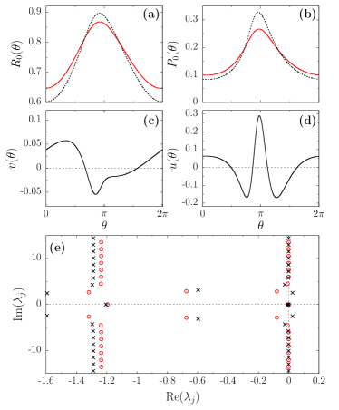
Figure 5: (a,b) Shapes of $R_{0}(\theta)$ and $P_{0}$ for $K=0.413$ (red) and $0.414$ (black dashed) obtained by solving Eqs. (9,10). (c,d) Shape of the unstable eigenfunction $v(\theta)$ and $u(\theta)$ for $K=0.414$. (e) Eigenvalues resulting from diagonalizing the linear equations (11) and (12) with $M=400$ Fourier modes for $K=0.413$ (red circles) and $0.414$ (black crosses).

V Increasing dynamical complexity

An analytical study of time-dependent nonlinear regimes is typically unfeasible. So, from now on, we proceed exclusively on a numerical basis, by relying on the integration of both microscopic and macroscopic equations. The Poincaré section is a qualitative but informative tool to understand the dynamical properties of the different regimes observed for larger values of $K$. It was already used in Nakagawa and Kuramoto (1995). Here we consider different observables for reasons that will be clear in a moment. More precisely, we introduce the collective variables

$$Z_{n}^{(k)}=\left|\int_{0}^{2\pi}d\psi R(\psi,t_{n})P(\psi,t_{n})\mathrm{e}^{ik\psi}\right|$$

where $t_{n}$ is the time at which $|\overline{z}|$ reaches a local maximum. This definition is basically an extension of the order parameters typically used to characterize phase oscillators, where the radial contribution $R$ is, for obvious reasons, absent. In phase oscillators, the $Z^{(k)}$ parameters are functionally related to one another whenever the Ott-Antonsen Ansatz is valid Ott and Antonsen (2008). It is therefore instructive to look at their mutual relationship.

In Fig. 6(a), we plot $Z_{n}^{(1)}$ versus $K$. Since the Poincaré section reduces by one unit the dimensionality of the underlying attractor, a periodic collective dynamics manifests itself as a single point for a given $K$ value. This is indeed what we see for $K<K_{3}$, although we should notice that the initial section of the curve corresponds to SCPS, where the order parameter is strictly constant. The fuzzy region covered for $K>K_{3}$ corresponds to a tiny interval where a T3 dynamics initially unfolds, followed by a chaotic regime, analyzed in more quantitative way in the second part of this section.

The lower panels of Fig. 6 contain various Poincaré section in the T3 region (blue dots) and in the chaotic region (red dots). The points have been obtained by integrating the macroscopic equations. Analogous pictures have been obtained by integrating 32768 oscillators, but significantly blurred by finite-size effects. The main message that we learn by comparing the three Poincaré sections is that there is no functional dependence among the first three order parameters, thus suggesting that they are really independent variables – an indirect evidence that the Watanabe-Strogatz theorem does not apply to this context.

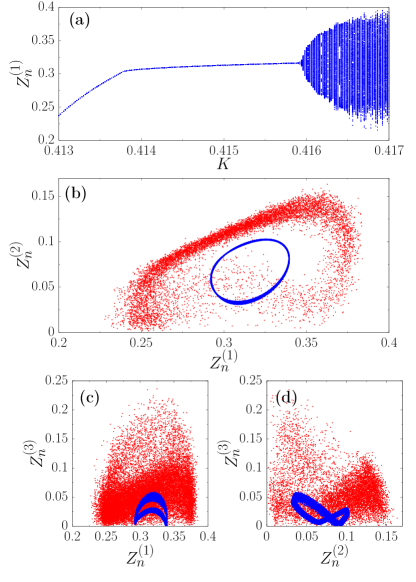
Figure 6: (a) Poincaré map of $Z_{n}^{(1)}$ for different values of the coupling strength $K$ computed using macroscopic simulations. The T1 and T2 regimes appear as stable fixed points, and T3 emerges through a Hopf-bifurcation. Simulations computed along $2\times 10^{4}$ time units after discarding a transient of $5\times 10^{5}$ time units. (b-d) Poincaré sections resulting from macroscopic simulations for $K=0.416$ (blue dots) and $K=0.4165$ (red dots). Simulations computed along $10^{5}$ time units after discarding a transient of $5\times 10^{4}$ time units.

How irregular is the regime which settles beyond $K_{4}$? How does chaos emerge? Obtaining a clean answer turned out to be arduous. In fact, one has to deal with: (i) long transients; (ii) the spontaneous formation of metastable states; (iii) finite-size effects (in microscopic simulations); (iv) the sporadic formation of highly localized, cluster-like structures (in macroscopic simulations). All of them required much care and long lasting simulations.

We first focus on the computation of the standard, microscopic, Lyapunov exponents. $N=4096$ turns out to be sufficiently large to ensure negligible finite-size corrections. The convergence is nevertheless very slow and a good way to cope with it is by launching simulations from different initial conditions. Moreover, we also add a small heterogeneity of the order of $10^{-14}$ among the oscillators in order to prevent the formation of spurious clusters due to the finite floating point representation. The parameter dependence of the first three Lyapunov exponents is summarized in Fig. 7. The three exponents appear to become positive for approximately the same coupling strength $K_{4}\approx 0.4161\ldots$. This is a first indication that we are before a new transition to chaos. It differs from the typical transitions to low-dimensional chaos (period doubling, intermittency, quasiperiodicity), which are accompanied by the change of sign of a single exponent. On the other hand, there is no similarity with the transitions expected in high-dimensional systems, such as spatio-temporal intermittency, where a bunch of exponents becomes positive, whose numerosity is proportional to the system size Chaté and Manneville (1987): a typical signature of extensivity.

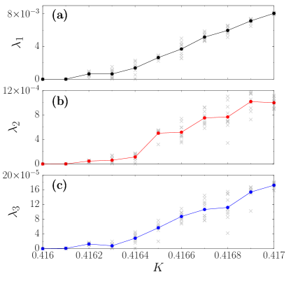
Figure 7: The three largest Lyapunov exponents of the microscopic system computed over different values of the coupling strength $K$. Circles indicate the average over ten different realizations, each starting from a different initial condition. Gray crosses show the outcome of the different single realizations. Each simulation consists of $N=4096$ oscillators, with a quenched disorder of the order of $10^{-14}$. The total computation time is of $10^{7}$ time units, of which $10^{5}$ are transient. Simulations computed using fourth order Runge-Kutta with time step $dt=0.01$. The Gram-Schmidt orthogonalization is invoked every 10 time steps.

A more detailed representation of the overall degree of instability is given in Fig. 8, where we plot the first 10 Lyapunov exponents deeply inside the chaotic region. All exponents beyond the third one are practically equal to zero. As a result, by virtue of the Kaplan-Yorke formula, the underlying attractor is characterized by a large (possibly infinite in the thermodynamic limit) dimension, in spite of the presence of just three positive exponents: an additional reason to classify this regime as genuinely new.

How does the microscopic instability compare to the macroscopic dynamics? In Fig. 8, we plot also the macroscopic Lyapunov exponents, obtained by linearizing the evolution equations (2,3,4) along a generic trajectory. In spite of the large fluctuations (especially those affecting the maximum exponent), the macroscopic spectrum is very similar to the microscopic one. This correspondence is far from obvious and shall be addressed in the final part of this section. Here, we want to stress that the presence of positive macroscopic exponents shows that we are before a form of collective chaos.

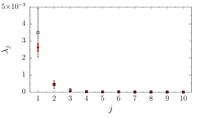
Figure 8: The 10 largest Lyapunov exponents for $K=0.4165$ computed using microscopic (red circles) and macroscopic (open black squares) simulations. The different points show the average over 10 (microscopic) and 50 (macroscopic) simulations starting from different initial conditions, with error bars indicating the standard deviation. Macroscopic simulations computed over $2\times 10^{4}$ time units after discarding a transient of $5\times 10^{3}$. Parameters for microscopic simulations as in figure 7.

In all mean-field models so far investigated in the literature, collective chaos is accompanied by the instability of the single dynamical units, which can be quantified by interpreting the mean field as an external driving force and thereby determining the so-called transverse Lyapunov exponent $\lambda_{T}$. This is the case of logistic maps Shibata and Kaneko (1998) as well as of Stuart-Landau oscillators in a different parameter region Takeuchi and Chaté (2013). From now on, we refer to this regime as to standard collective chaos (SCC). We now show that the collective dynamics observed beyond $T3$ has a different nature.

In the present context, $\lambda_{T}$ can be determined by linearizing the evolution equation (1) under the assumption that $\bar{z}(t)$ is an external forcing,

$$\dot{u}=[1-K(1+ic_{1})]u-(1+ic_{2})z(2z^{*}u+zu^{*})\;,$$ (14)

where $u$ denotes an infinitesimal perturbation of $z$. This equation being two-dimensional ($u$ is a complex variable) is characterized by two (transverse) Lyapunov exponents. The lower exponent is unavoidably negative (in the present case it expresses the stability of deviations from the time-dependent curve $\mathcal{C}$). Less trivial is the value of the largest transverse exponent $\lambda_{T}$, which quantifies the stability of perturbations aligned with the tangent to the curve ($\mathcal{C}$). The best way to describe the underlying phenomenology is by invoking the standard multifractal formalism, which takes into account the fluctuations of the Lyapunov exponents (see, e.g., the book Pikovsky and Politi (2016)). Let us start by introducing the generalized Lyapunov exponent

$$\mathcal{L}(q)=\lim_{\tau\to\infty}\frac{1}{q\tau}\ln\langle|H(\tau)u|^{q}\rangle$$

where $H$ represents the Jacobian integrated over a time $\tau$ (from Eq. (14)). $\mathcal{L}(0)$ corresponds to the standard the Lyapunov exponent, while $\mathcal{L}(1)$ corresponds to the topological entropy (in case there is a single positive exponent) . In fact, $\mathcal{L}(1)$ yields the expansion rate of an arc of initial conditions initially aligned along the most expanding direction. In the current context, the orientation of the arc corresponds to that of the curve $\mathcal{C}$. Since the curve itself has a fluctuating but finite length, the length of any subsegment does neither grow nor diverge in time, so that $\mathcal{L}(1)=0$.

The generalized Lyapunov exponents can be determined from the probability $\mathcal{P}(\Lambda,\tau)$ to observe a finite-time Lyapunov exponent $\Lambda$ over a time $\tau$ and thereby introducing the large deviation function $S(\Lambda)$

$$S(\Lambda)=\lim_{\tau\to\infty}-\frac{\ln\mathcal{P}(\Lambda,\tau)}{\tau}\;.$$

The function $S(\Lambda)$ is equivalent to $\mathcal{L}(q)$, the connection between the two representations being given by the Legendre-Fenchel transform Pikovsky and Politi (2016)

$$q\mathcal{L}(q)=q\Lambda^{*}-S(\Lambda^{*})\;,$$

where $q=S^{\prime}(\Lambda^{*})$. In the Gaussian approximation

$$S(\Lambda)=\frac{(\Lambda-\lambda_{T})^{2}}{2D}$$

where $\lambda_{T}$ is the standard transverse Lyapunov exponent, while $D$ is the corresponding diffusion coefficient defined as

$$D=\lim_{\tau\to\infty}\tau\left(\overline{\Lambda(\tau)^{2}}-\lambda_{T}^{2}\right)\;.$$

As a result, we eventually find that

$$\mathcal{L}(1)=\lambda_{T}+\frac{D}{2}\;.$$ (15)

Both $\lambda_{T}$ and $D$ can be determined from the time evolution of $\gamma(\tau)=\tau\Lambda(\tau)$. In fact, $\gamma(\tau)$ is the logarithm of the expansion factor over a time $\tau$; it is basically a Brownian motion with a drift velocity $\lambda_{T}$ and a diffusion coefficient $D$. For $K=0.4165$, upon integrating over $10^{7}$ time units we find a slightly negative Lyapunov exponent $\lambda_{T}\approx(-1.7\pm 0.6)\times 10^{-5}$, while $D\approx(4.4\pm 0.3)\times 10^{-5}$. As a result, from Eq. (15), $\mathcal{L}(1)\approx(0.5\pm 0.75)\times 10^{-5}$, a value compatible with the expected vanishing exponent. In other words, we see that the fluctuations of the finite-time Lyapunov exponent compensate the slightly negative $\lambda_{T}$ and ensure a vanishing expansion factor for the curve length.

Altogether, the message arising from the multifractal analysis is that the (unavoidable) fluctuations of the transverse Lyapunov exponent induce a set of singularities for the corresponding probability density (in the regular SCPS, there are no fluctuations of the Lyapunov exponent, which is identically equal to 0).

A posteriori, this observation accounts for the difficulties encountered in our simulations of the chaotic phase: in fact, the formation of temporary clusters which so much affect the accuracy of our simulations, irrespective whether they are carried out at the microscopic or macroscopic level, are nothing but a manifestation of the unavoidable presence of singularities, which are intrinsically associated to the self-sustainment of a fluctuating probability density.

We conclude this section by commenting on the similarity between macroscopic and microscopic Lyapunov spectra. The correspondence is unexpected since they arise from two different descriptions of the world. In the microscopic approach, the key variables are the “positions” of the single oscillators, while the macroscopic approach deals with their distribution in phase space. Imagine, for simplicity, to deal with $N$ particles constrained to move along a given curve of fixed length: a virtually infinitesimal microscopic perturbation corresponds to a shift of each particle over a scale that is by definition small compared to the interparticle distance, of the order of $1/N$. On the other hand, to meaningfully interpret a perturbation of the positions as a perturbation of the corresponding probability density, it must occur on a scale larger than the statistical fluctuations, which is of order $\sqrt{1/N}$. A priori, there is no guarantee that the linearization of the microscopic equations still hold over such “large scales” (see Ref. Politi et al. (2017), for a more detailed discussion of this point). In fact, in typical instances of SCC, macroscopic and microscopic Lyapunov spectra substantially differ from one another. In the toy model of SCC discussed in Politi et al. (2017), the collective dynamics is characterized by a single positive macroscopic exponent, while the number of positive exponents is proportional to the number of oscillators, in the microscopic dynamics. The main point of discussion is whether and when some of the microscopic exponents “percolate” to the macroscopic level. In Ref. Takeuchi and Chaté (2013) it is conjectured that this happens whenever the corresponding covariant Lyapunov vector has an extensive nature, but it is still unclear under which conditions this opportunity materializes.

So, what is the difference with the collective chaos discussed in this paper? The stability analysis of splay states in leaky integrate-and-fire (LIF) neurons can help to shed some light. At the collective level, the state splay corresponds to a trivial staionary homegeneous distribution and its stability can be studied by diagonalizing the corresponding linearized evolution operator. This step was already performed in the early’90s, determining an analytical expression of the entire spectrum in the weak coupling limit Abbott and van Vreeswijk (1993). More recently, the same problem was revisited from the microscopic point of view, analyzing an arbitrary number $N$ of neurons Olmi et al. (2014), finding that the leading exponents progressively approach the macroscopic ones (upon increasing $N$), analogously to what observed in Fig. 8. The main difference between splay states and SCC is the absence of microscopic chaos and thereby the absence of the statistical fluctuations of size $1/\sqrt{N}$ which would otherwise represent a sort of “barrier” separating the microscopic from the macroscopic world (see Politi et al. (2017) for additional considerations of this point). The maintanance of ordering observed in the collective chaos discussed in this paper, makes it closer to the splay state than to SCC.

VI Conclusions and open problems

In this paper we have developed a formalism that allows characterizing an intermediate regime where amplitude oscillators keep some phase-oscillator properties (i.e. the alignment along a smooth curve), while starting to exhibit nontrivial amplitude oscillations. Our analysis deals with Stuart-Landau oscillators, but nothing precludes the application of the same formalism to generic oscillators, in so far as their evolution remains confined to a smooth curve $\mathcal{C}$.

We show that SCPS is a generic regime: a necessary condition for it to be self-sustained is the presence of more than one Fourier harmonics in the effective coupling function, a property that is here induced by the amplitude dynamics. Our formalism allows for an almost analytical characterization of SCPS and, in particular, to determine the bifurcation point, beyond which complex time-dependent states arise. If SCPS is by itself a non-intuitive regime, since the single oscillators behave quasi-periodically without displaying any locking phenomena, the chaotic SCPS described in section V is even more so. Each oscillator, under the action of the self-sustained chaotic mean-field, is consistently marginally stable (the transversal generalized Lyapunov exponent being equal to zero for $q=1$) when the coupling strength is varied. An implication of this observation is that the probability density is unavoidably characterized by the presence of singularities that manifest themselves as temporary clusters.

If and when the transversal Lyapunov exponent becomes positive, a transition to SCC occurs, accompanied by the divergence of the curve $\mathcal{C}$, which would thereby “fill” the phase space (in a fractal way). In the parameter range explored in this paper, this transition is preceded by the onset of a non-conventional incoherent state (i.e. nonuniform distribution characterized by a zero order parameter), which restores a perfectly circular shape of $\mathcal{C}$. It will be worth clarifying the possibly universal mechanisms that may lie behind such a kind of transition.

Finally, the onset of a chaotic SCPS is itself an entirely new phenomenon which involves the simultaneous emergence of more than one positive Lyapunov exponent (actually it looks like three of them). While we could imagine simple mechanisms for the emergence of discontinuous changes (see, e.g. attractor crises), the justification of a continuous transition such as the one discussed in this paper is by far more intriguing. Last but not least, the question whether chaotic SCPS can be observed in perfect phase oscillators remains open.

Appendix A First order approximation of SCPS

In this section we develop a perturbative approach to determine the stationary solutions of Eqs. (9,10) close to the transition to SCPS, $K\sim K_{1}$. The main idea is, as usual, the identification of the leading terms. Slightly above $K_{1}$, the shape $R_{0}$ of the attractor and the corresponding density distribution $P_{0}$ of the phases are close to the splay state, so that we can write

$$R_{0}(\theta) = \sqrt{1-K}+r(\theta)$$ (16)

$$P_{0}(\theta) = \frac{1}{2\pi}+p(\theta)\;.$$

Expanding the self-consistent condition (8) up to linear terms, we obtain

$$\bar{z} =\int_{0}^{2\pi}d\psi P(\psi)R(\psi)e^{i\theta}$$

$$=\frac{1}{2\pi}\int_{0}^{2\pi}e^{i\psi}d\psi r(\psi)+\sqrt{1-K}\int_{0}^{2\pi}d\psi p(\psi)\mathrm{e}^{i\psi}$$

$$=\frac{1}{2\pi}\tilde{r}(1)+\sqrt{1-K}\tilde{p}(1)\;.$$ (17)

By then expanding equation (9) up to first order, one obtains

$$[r(\theta)]_{\theta}=\frac{2(1-K)r-K\bar{z}\sqrt{1+c_{1}^{2}}\cos(\nu-\theta)}{\Delta}\;,$$

where

$$\Delta:= \omega+c_{1}K+c_{2}(1-K)\;,$$

$$\nu:= \arctan c_{1}$$

By introducing the notations

$$a_{\xi}\mathrm{e}^{i\xi}:= \frac{2(1-K)}{\Delta}-i,$$

$$A:= \frac{K\sqrt{1+c_{1}^{2}}}{a_{\xi}\Delta},$$

one can write the solution of the ODE as

$$r(\theta)=\overline{z}A\cos(\nu+\xi-\theta)\;.$$ (18)

Accordingly,

$$\tilde{r}(1)=\pi\overline{z}A\mathrm{e}^{i(\nu+\xi)}$$

By expanding Eq. (10) in the same way, at zero order we obtain

$$\eta=-\frac{\Delta}{2\pi}$$

while, at first order,

$$p(\theta)=\frac{-2c_{2}(1-K)r(\theta)+K\bar{z}\sqrt{1+c_{1}^{2}}\sin(\nu-\theta)}{2\pi\Delta\sqrt{1-K}}$$

By replacing the expression for $r(\theta)$,

$$p(\theta)=C\bar{z}\left[-\frac{2c_{2}(1-K)}{a_{\xi}\Delta}\cos(\nu+\xi-\theta)+\sin(\nu-\theta)\right]$$

where

$$C=\frac{K}{2\pi\Delta}\sqrt{\frac{1+c_{1}^{2}}{1-K}}\;.$$

By finally, recombining the two sinusoidal terms, we find

$$p(\theta)= a_{\gamma}C\bar{z}\cos(\nu+\gamma-\theta)$$

where

$$a_{\gamma}\mathrm{e}^{i\gamma}=\frac{-2(1-K)c_{2}\mathrm{e}^{i\xi}}{a_{\xi}\Delta}-i\;.$$

Thus, also $p(\theta)$ is a purely harmonic function and

$$\tilde{p}(1)=\pi\overline{z}a_{\gamma}C\mathrm{e}^{i(\nu+\gamma)}\;.$$

The overall effect of the coupling is finally determined by inserting the expressions for $\tilde{r}(1)$ and $\tilde{p}(1)$ into Eq. (A). Since both terms are proportional to $\bar{z}$, we can interpret

$$G:=g_{z}\mathrm{e}^{i\delta}:=\frac{A}{2}\mathrm{e}^{i(\xi+\nu)}+\pi a_{\gamma}C\sqrt{1-K}\mathrm{e}^{i(\gamma+\nu)}\;,$$

as the expansion factor of $\bar{z}$ in the presence of a given small modulation of both $\mathcal{C}$ and the probability density. Imposing $G=1$ finally allows determining a self-consistent solution. More precisely, one can determine the frequency $\omega$ of the collective rotation (so far unspecified) and the bifurcation point $K$. For $c_{1}=-2$ and $c_{2}=3$, we obtain $K=K_{1}\simeq 0.4123...$ and $\omega=\omega_{c}=-2.5261...$, i.e., in agreement with the stability analysis of the splay state.

Appendix B Stability of SCPS

The coefficients of the linearized equations (11,12) are

$$F^{(v)}(\theta):= (1-K)-3R_{0}(\theta)^{2}+2c_{2}R_{0}^{\prime}(\theta)R_{0}(\theta)$$

$$\quad+\frac{K\overline{z}R_{0}^{\prime}(\theta)}{R^{2}_{0}(\theta)}\sqrt{1+c_{1}^{2}}\sin(\nu-\theta)\;,$$

$$G^{(v)}(\theta):= Kc_{1}+\omega+c_{2}R_{0}^{2}-\frac{K\overline{z}}{R_{0}(\theta)}\sqrt{1+c_{1}^{2}}\sin(\nu-\theta)\;,$$

$$X^{(v)}(\theta):= \frac{K\sqrt{1+c_{1}^{2}}}{2}\left(1-\frac{R_{0}^{\prime}(\theta)}{iR_{0}(\theta)}\right)e^{i(\nu-\theta)}\;,$$

$$Y^{(v)}(\theta):= \frac{K\sqrt{1+c_{1}^{2}}}{2}\left(1+\frac{R_{0}^{\prime}(\theta)}{iR_{0}(\theta)}\right)e^{-i(\nu-\theta)}\;,$$

$$F^{(u)}(\theta):= 2c_{2}P_{0}(\theta)R_{0}(\theta)+\frac{KP_{0}(\theta)\overline{z}}{R_{0}(\theta)^{2}}\sqrt{1+c_{1}^{2}}\sin(\nu-\theta)\;,$$

$$G^{(u)}(\theta):= Kc_{1}+\omega+c_{2}R_{0}(\theta)^{2}-\frac{K\overline{z}}{R_{0}(\theta)}\sqrt{1+c_{1}^{2}}\sin(\nu-\theta)\;,$$

$$X^{(u)}(\theta):= -\frac{KP_{0}(\theta)}{2iR_{0}(\theta)}\sqrt{1+c_{1}^{2}}e^{i(\nu-\theta)}\;,$$

$$Y^{(u)}(\theta):= \frac{KP_{0}(\theta)}{2iR_{0}(\theta)}\sqrt{1+c_{1}^{2}}e^{-i(\nu-\theta)}\;.$$

The equations are better solved in Fourier space. By invoking the Fourier transform, the integrals in the linearized mean-field expression (IV.1) can be expanded as a linear combination of $\{\tilde{v}(k,t)\}_{k=-\infty}^{\infty}$ and $\{\tilde{u}(k,t)\}_{k=-\infty}^{\infty}$,

$$w(t)=\frac{1}{2\pi}\sum_{k=-\infty}^{\infty}\tilde{v}(k)\tilde{P}_{0}(1-k)+\tilde{u}(k)\tilde{R}_{0}(1-k)$$

and

$$\hat{w}(t)=\frac{1}{2\pi}\sum_{k=-\infty}^{\infty}\tilde{v}(k)\tilde{P}_{0}(-1-k)+\tilde{u}(k)\tilde{R}_{0}(-1-k).$$

Similarly, we express Eqs. (11) and (12) in Fourier space. Retaining the terms for each wavelength $k$ we obtain an infinite system of linear equations,

$$[\tilde{v}(k)]_{t} =\frac{1}{2\pi}\sum_{j=-\infty}^{\infty}\tilde{v}(j)\Bigl{[}\tilde{F}^{(v)}(k-j)-ij\tilde{G}^{(v)}(k-j)$$

$$+\tilde{X}^{(v)}(k)\tilde{P}_{0}(1-j)+\tilde{Y}^{(v)}(k)\tilde{P}_{0}(-1-j)\Bigr{]}$$

$$+\tilde{u}(j)\Bigl{[}\tilde{X}^{(v)}(k)\tilde{R}_{0}(1-j)+\tilde{Y}^{(v)}(k)\tilde{R}_{0}(-1-j)\Bigr{]}$$

and

$$[\tilde{u}(k)]_{t} =\frac{-ik}{2\pi}\sum_{j=-\infty}^{\infty}\tilde{v}(j)\Bigl{[}\tilde{F}^{(u)}(k-j)$$

$$+\tilde{X}^{(u)}(k)\tilde{P}_{0}(1-j)+\tilde{Y}^{(u)}(k)\tilde{P}_{0}(-1-j)\Bigr{]}$$

$$+\tilde{u}(j)\Bigl{[}\tilde{G}^{(u)}(k-j)+\tilde{X}^{(u)}(k)\tilde{R}_{0}(1-j)$$

$$+\tilde{Y}^{(u)}(k)\tilde{R}_{0}(-1-j)\Bigr{]}\;.$$

References

- Note (1) The term “collective” is often used to refer to the behavior of an ensemble of units induced by mutual coupling. Here we use it to refer, as in statistical-mechanics, to macroscopic features exhibited by observables averaged over a formally infinite number of contributions.
- Golomb et al. (1992) D. Golomb, D. Hansel, B. Shraiman, and H. Sompolinsky, “Clustering in globally coupled phase oscillators,” Phys. Rev. A 45, 3516–3530 (1992).
- Kuramoto and Battogtokh (2002) Y. Kuramoto and D. Battogtokh, “Coexistence of coherence and incoherence in nonlocally coupled phase oscillators,” Nonlinear Phenomena in Complex Systems 5, 180 (2002).
- Abrams and Strogatz (2004) Daniel M. Abrams and Steven H. Strogatz, “Chimera states for coupled oscillators,” Phys. Rev. Lett. 93, 174102 (2004).
- Kaneko (1990) Kunihiko Kaneko, “Globally coupled chaos violates the law of large numbers but not the central-limit theorem,” Phys. Rev. Lett. 65, 1391–1394 (1990).
- Nakagawa and Kuramoto (1993) Naoko Nakagawa and Yoshiki Kuramoto, “Collective chaos in a population of globally coupled oscillators,” Progress of Theoretical Physics 89, 313 (1993).
- Vincent Hakim (1992) Wouter-Jan Rappel Vincent Hakim, “Dynamics of the globally coupled complex ginzburg-landau equation,” Physical Review A 46, 7347–7350 (1992).
- Marie-Line Chabanol (1997) Wouter-Jan Rappel Marie-Line Chabanol, Vincent Hakim, “Collective chaos and noise in the globally coupled complex ginzburg-landau equation,” Physica D 103, 273–293 (1997).
- Pazó and Montbrió (2016) Diego Pazó and Ernest Montbrió, “From quasiperiodic partial synchronization to collective chaos in populations of inhibitory neurons with delay,” Phys. Rev. Lett. 116, 238101 (2016).
- Olmi et al. (2010) S. Olmi, A. Politi, and A. Torcini, “Collective chaos in pulse-coupled neural networks,” EPL (Europhysics Letters) 92, 60007 (2010).
- Luccioli and Politi (2010) Stefano Luccioli and Antonio Politi, “Irregular collective behavior of heterogeneous neural networks,” Phys. Rev. Lett. 105, 158104 (2010).
- van Vreeswijk (1996) C. van Vreeswijk, “Partial synchronization in populations of pulse-coupled oscillators,” Phys. Rev. E 54, 5522–5537 (1996).
- Mohanty and Politi (2006) P.K. Mohanty and A. Politi, “A new approach to partial synchronization in globally coupled rotators,” J. Phys. A: Math. Gen. 39, L415–L421 (2006).
- Rosenblum and Pikovsky (2007) Michael Rosenblum and Arkady Pikovsky, “Self-organized quasiperiodicity in oscillator ensembles with global nonlinear coupling,” Phys. Rev. Lett. 98, 064101 (2007).
- Pikovsky and Rosenblum (2009) Arkady Pikovsky and Michael Rosenblum, “Self-organized partially synchronous dynamics in populations of nonlinearly coupled oscillators,” Physica D: Nonlinear Phenomena 238, 27 – 37 (2009).
- Politi and Rosenblum (2015) Antonio Politi and Michael Rosenblum, “Equivalence of phase-oscillator and integrate-and-fire models,” Phys. Rev. E 91, 042916 (2015).
- Rosenblum and Pikovsky (2015) M. Rosenblum and A. Pikovsky, “Two types of quasiperiodic partial synchrony in oscilator ensembles,” Phys. Rev. E 92, 012919 (2015).
- Clusella et al. (2016) Pau Clusella, Antonio Politi, and Michael Rosenblum, “A minimal model of self-consistent partial synchrony,” New Journal of Physics 18, 093037 (2016).
- E. Ullner (2018) A. Torcini E. Ullner, A. Politi, “Ubiquity of collective irregular dynamics in balanced networks of spiking neurons,” CHAOS 28, 081106 (2018).
- Watanabe and Strogatz (1993) S. Watanabe and S. H. Strogatz, “Integrability of a globally coupled oscillator array,” Phys. Rev. Lett. 70, 2391–2394 (1993).
- Ott and Antonsen (2008) Edward Ott and Thomas M. Antonsen, “Low dimensional behavior of large systems of globally coupled oscillators,” Chaos 18, 037113 (2008).
- Nakagawa and Kuramoto (1995) Naoko Nakagawa and Yoshiki Kuramoto, “Anomalous lyapunov spectrum in globally coupled oscillators,” Physica D: Nonlinear Phenomena 80, 307 – 316 (1995).
- Takeuchi and Chaté (2013) Kazumasa A Takeuchi and Hugues Chaté, “Collective lyapunov modes,” Journal of Physics A: Mathematical and Theoretical 46, 254007 (2013).
- Sakaguchi and Kuramoto (1986) H. Sakaguchi and Y. Kuramoto, “A soluble active rotator model showing phase transition via mutual entrainment,” Prog. Theor. Phys. 76, 576–581 (1986).
- Sethia and Sen (2014) Gautam C. Sethia and Abhijit Sen, “Chimera states: The existence criteria revisited,” Phys. Rev. Lett. 112, 144101 (2014).
- Canuto et al. (2006) C. Canuto, M.Y. Hussaini, A. Quarteroni, and Th.A. Zang, Spectral Methods: Fundamentals in Single Domains, 1st ed., Can (Springer-Verlag, Berlin, 2006) Chap. 2.
- Note (2) The obfuscation of blue points clearly visible in panels (c) and (d) of Fig. 6 are also artifacts due to the finite accuracy in the determination of the Poincaré section.
- Chaté and Manneville (1987) Hugues Chaté and Paul Manneville, “Transition to turbulence via spatio-temporal intermittency,” Phys. Rev. Lett. 58, 112–115 (1987).
- Shibata and Kaneko (1998) Tatsuo Shibata and Kunihiko Kaneko, “Tongue-like bifurcation structures of the mean-field dynamics in a network of chaotic elements,” Physica D: Nonlinear Phenomena 124, 177 – 200 (1998).
- Pikovsky and Politi (2016) Arkady Pikovsky and Antonio Politi, Lyapunov Exponents: A Tool to Explore Complex Dynamics (Cambridge University Press, 2016).
- Note (3) We warn the reader that a different definition is often found in the literature, where corresponds to the standard Lyapunov exponent. Here we follow the same notations as in Pikovsky and Politi (2016).
- Note (4) Here, denotes the finite-time Lyapunov exponent computed by following a single trajectory from time 0 to time .
- Politi et al. (2017) Antonio Politi, Arkady Pikovsky, and Ekkehard Ullner, “Chaotic macroscopic phases in one-dimensional oscillators,” The European Physical Journal Special Topics 226, 1791–1810 (2017).
- Abbott and van Vreeswijk (1993) L. F. Abbott and Carl van Vreeswijk, “Asynchronous states in networks of pulse-coupled oscillators,” Phys. Rev. E 48, 1483–1490 (1993).
- Olmi et al. (2014) Simona Olmi, Antonio Politi, and Alessandro Torcini, “Linear stability in networks of pulse-coupled neurons,” Frontiers in Computational Neuroscience 8, 8 (2014).