SU(2)${}_{\text{\tiny{{CMB}}}}$ and the cosmological model:
angular power spectra

Abstract

Driven by the CMB temperature-redshift ($T$-$z$) relation as demanded by deconfining SU(2) Yang-Mills thermodynamics, an according cosmological model is proposed and analysed. This model – SU(2)${}_{\textnormal{\tiny{cmb}}}$ – exhibits a dark sector, representing $\Lambda$CDM with a certain late-time dark-matter density which transitions to a reduced (present-day) density parameter at high $z$. We statistically analyse constraints on cosmological parameters directly imposed by the values of the standard co-moving ruler $r_{d}$ and the angular size of the sound horizon $\theta_{*}$. Compared to the $\Lambda$CDM best fit to 2015 Planck data, we require an increased (present-day) dark matter density when $r_{d}\cdot H_{0}=$ const and a value $H_{0}\sim 73.5$ km s^-1Mpc^-1 – typical for local extractions – are used. The ratio between the density parameters of primordial and late-time dark matter ranges between 0.5 and 0.7. We confirm this trend by fitting the predictions of SU(2)${}_{\textnormal{\tiny{cmb}}}$, obtained from a modified CLASS code, to the angular power spectra TT, TE, and EE. We consider adiabatic, scalar primordial curvature perturbations and distinguish two treatments of thermal quasi-particles in the perturbation equations. Best fits predict a red-tilted primordial power spectrum. Moreover, a low baryon density is obtained compared with the coincidence value of BBN, the $\Lambda$CDM best fit of the 2015 Planck data, and the observed deuterium abundance. Our derived values of $H_{0}$ support the results of local cosmological observations. Also, there is a tendency for late reionisation. Pdflatex could not properly compile abstracts with less than 1700 characters?!????????????

1 Introduction

The last two and a half decades have converted cosmology into a precision science, resulting in independent data sets which constrain models of our universe: (i) large-scale structure surveys of the matter correlation function, suggesting the existence of a standard ruler $r_{d}$ set by the physics of baryonic acoustic oscillations, e.g., Abazajian et al. (2003); Adelman-McCarthy et al. (2008), (ii) observations of the temperature and polarisation fluctuations in the CMB Mather et al. (1990); Hinshaw et al. (2013) with a high angular resolution Ade et al. (2014a, 2016) by satellite based missions, and (iii) use of calibrated SNe Ia in distance-redshift surveys, ultimately changing the paradigm on the rate of late-time (low-$z$) expansion Perlmutter et al. (1998); Riess et al. (1998).

The $\Lambda$CDM concordance model fits most of the cosmological data in a satisfactory way. In particular, the accelerated expansion of the universe at late times due to the dominance of dark energy as well as the spatial flatness of the universe de Bernadis et al. (2000) can be considered secured facts. However, recent results reveal a considerable tension between the high value of the present expansion rate $H_{0}=73.48\pm 1.66$ km s^-1Mpc^-1 extracted from calibrated distances to SNe Ia (local observation Riess et al. (2018); Cardona et al. (2017)) and the low values $H_{0}=66.93\pm 0.62$ km s^-1Mpc^-1 obtained from the 2015 Planck data or $H_{0}=69.1^{+0.4}_{-0.6}$ km s^-1Mpc^-1 from the clustering of galaxies (global observations Aghanim et al. (2016); Abbott et al. (2017)). An independent distance estimator, appealing to time delays from gravitational lensing, extracts a high value of $H_{0}=72.8\pm 2.4$ km s^-1Mpc^-1 (local observation Bonvin et al. (2017)). The discrepancy between the local and the global values of $H_{0}$ is unlikely to be resolved by sample variance, local matter-density fluctuations, or a directional bias in SNe Ia observations Marra et al. (2013); Odderskov, Hannestad & Haugbølle (2014); Odderskov, Hannestad & Brandbyge (2017); Wu & Huterer (2017): their effect $\Delta H_{0}\sim 0.31$ km s^-1Mpc^-1 is much smaller than the local-global discrepancy $\Delta H_{0}\sim 6$ km s^-1Mpc^-1.

In Hahn & Hofmann (2017) a modification of the high-redshift cosmological model, dubbed SU(2)${}_{\textnormal{\tiny{cmb}}}$, was proposed. In this model the U(1) gauge group of electromagnetism is replaced by an SU(2) gauge principle (Yang-Mills theory), motivated theoretically in Hofmann (2016a) and observationally by an excess of CMB line temperatures at low frequencies, see Fixsen et al. (2011); Hofmann (2009) and references therein. The work Hahn & Hofmann (2017) mainly was concerned with high-$z$ implications of this model for the co-moving sound horizon at baryon drag $r_{d}$, in turn fixing the value of $H_{0}$ Bernal, Verde & Riess (2016). In analysing this model further towards its implications for the CMB angular power spectra, the present authors have noticed a number of oversights in Hahn & Hofmann (2017). Namely, the parameter $R_{{\rm SU(2)}_{\textnormal{\tiny{cmb}}}}$, governing the sound velocity in the baryon-Yang-Mills plasma, was defined conventionally which violates energy-conservation in the extended situation. Also, the dark-sector model turns out to be too radical in excluding primordial dark matter all together. In the present work these shortcomings are eliminated. We now demonstrate SU(2)${}_{\textnormal{\tiny{cmb}}}$’s potential to resolve the tension in $H_{0}$ between local cosmology and $\Lambda$CDM fits to the 2015 Planck data. Our present findings favour a late reionisation as suggested by observation of the Gunn-Peterson trough in the spectra of distant quasars Becker et al. (2001). However, these encouraging results are at the expense of admitting a red-tilted spectrum of primordial adiabatic, scalar curvature perturbations, a high matter density, and a low baryon density.

This work is organised as follows. In Sec. 2 we introduce the cosmological model SU(2)${}_{\textnormal{\tiny{cmb}}}$. The pronounced modification of the dark sector in this model is driven by an unconventional $T$-$z$ relation in deconfining SU(2) Yang-Mills thermodynamics, assuming that the CMB is described by such a theory. In addition, the conversion between neutrino and CMB temperature is changed. We also briefly review linear cosmological perturbation theory in conformal Newtonian gauge with a special focus on issues arising in SU(2)${}_{\textnormal{\tiny{cmb}}}$ due to the emergence of a non-primordial dark-matter component and the additional gauge-mode degrees of freedom. To constrain the cosmological parameters we perform a statistical analysis in Sec. 3 by imposing the values of the angular size of the sound horizon $\theta_{*}$ and the standard co-moving ruler $r_{d}$. It turns out that these constraints only determine the total late-time and the primordial dark-matter densities while other parameters remain unfixed. In Sec. 4 computations of the angular power spectra of TT, TE, and EE as well as likelihood maximisations w.r.t. the 2015 Planck data are carried out after a short discussion of the modifications in CLASS modules. As a result, we obtain best fits (minima of co-profiles) which predict a red-tilted power spectrum of primordial, adiabatic, and scalar curvature perturbations, a low baryon density, and a high total-matter as well as dark-matter density at late times. We see good agreement of $H_{0}$ with local cosmological observation, and a tendency for a low redshift of reionisation $z_{\rm re}$, as extracted from spectral observations of distant quasars. These results are discussed in view of independent constraints. Finally, in Sec. 5 we summarize our results and sketch how the currently missing treatment of radiative effects at low $z$ could be implemented. We also emphasise the necessity of understanding the “microscopics" in the purported depercolation physics of the modified dark sector.

2 Modified cosmological model

Let us start by discussing the theoretical basis for SU(2)${}_{\textnormal{\tiny{cmb}}}$. For a detailed treatise of deconfining SU(2) Yang-Mills thermodynamics the reader may consult Ch. 5 of Hofmann (2016a), Hofmann (2009) for the observational fixation of the Yang-Mills scale (or critical temperature $T_{c}$), and Hofmann (2015); Hahn & Hofmann (2018) for the derivation of the CMB-temperature–redshift ($T$-$z$) relation. For the compatibility of this $T$-$z$ relation with existing data, such as the thermal Sunyaev-Zeldovich effect, see Hahn & Hofmann (2017).

We first introduce the cosmological model for the background evolution, assuming a spatially flat Friedmann-Lemaître-Robertson-Walker (FLRW) universe, also in regard to the computation of certain derived quantities like the co-moving sound horizon. This model comprises a modified dark sector which connects $\Lambda$CDM at low $z$ to a high-$z$ model. In addition, SU(2)${}_{\textnormal{\tiny{cmb}}}$ demands a modified $T$-$z$ relation as well as a change in the conversion between neutrino temperature $T_{\nu}$ and $T$. When addressing the first-order cosmological perturbations in SU(2)${}_{\textnormal{\tiny{cmb}}}$ we point out peculiarities surfacing in the Einstein-, Euler-, and Boltzmann equations. Moreover, the assumed (instantaneous) emergence of dark matter via the depercolation of Planck-scale axion vortices requires a modelling of the initial conditions with respect to its density contrast and its divergence of fluid velocity Ma & Bertschinger (1995).

2.1 Background model

2.1.1 Modified temperature-redshift relation

It is worthwhile to repeat the discussion of the $T$-$z$ relation in SU(2)${}_{\textnormal{\tiny{cmb}}}$, see also Hofmann (2015); Hahn & Hofmann (2018), because it implies changes for the dark-matter content at high $z$ Hahn & Hofmann (2017).

Demanding energy conservation in an FLRW universe the following equation is to be considered

$$\frac{\mbox{d}\rho_{\textnormal{\tiny{ym}}}}{\mbox{d}a}=-\frac{3}{a}\left(\rho_{\textnormal{\tiny{ym}}}+P_{\textnormal{\tiny{ym}}}\right)\,,$$ (1)

where $\rho_{\textnormal{\tiny{ym}}}$ and $P_{\textnormal{\tiny{ym}}}$ denote energy density and pressure, respectively, in the deconfining phase of SU(2) Yang-Mills thermodynamics (subscript ym). For later use, we associate the subscript l with the $\Lambda$CDM model, subject to conventional U(1) photon physics. Moreover, $a$ refers to the cosmological scale factor, normalised such that today $a(T_{0})=1$. Here, $T_{c}=T_{0}=2.725\,$K Hofmann (2009) indicates the present baseline temperature of the CMB Mather et al. (1990). Solving for $a$, the solution to Eq. (1) reads

$$a\equiv\frac{1}{z+1}=\exp\left(-\frac{1}{3}\log\left(\frac{s_{\textnormal{\tiny{ym}}}(T)}{s_{\textnormal{\tiny{ym}}}(T_{0})}\right)\right)\,,$$ (2)

where the entropy density $s_{\textnormal{\tiny{ym}}}$ is defined by

$$s_{\textnormal{\tiny{ym}}}\equiv\frac{\rho_{\textnormal{\tiny{ym}}}+P_{\textnormal{\tiny{ym}}}}{T}\,.$$ (3)

For $T\gg T_{0}$ Eq. (2) simplifies Hofmann (2016a) to

$$T=\left(\frac{1}{4}\right)^{1/3}T_{0}(z+1)\approx 0.63\,T_{0}(z+1)\,.$$ (4)

For arbitrary $T\geq T_{0}$ we define the multiplicative deviation $S(z)$ from linear scaling as

$${\cal S}(z)=\left(\frac{\rho_{\textnormal{\tiny{ym}}}(z=0)+P_{\textnormal{\tiny{ym}}}(z=0)}{\rho_{\textnormal{\tiny{ym}}}(z)+P_{\textnormal{\tiny{ym}}}(z)}\frac{T^{4}(z)}{T^{4}_{0}}\right)^{1/3}\,,$$ (5)

such that

$$T={\cal S}(z)\,T_{0}(z+1)\,.$$ (6)

Fig. 1 depicts function ${\cal S}(z)$.

Figure 1: The function ${\cal S}(z)$ of Eq. (5) which indicates the (multiplicative) deviation from the linear $T$-$z$ relation of Eq. (4). The curvature at low $z$ is due to the breaking of scale invariance in the deconfining SU(2) Yang-Mills plasma for $T\sim T_{0}=T_{c}$. Notice the rapid approach towards the asymptotics $\left(\frac{1}{4}\right)^{1/3}\approx 0.63$ with increasing $z$.

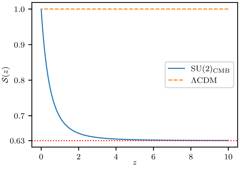
When the contribution of the thermal ground state in the deconfining SU(2) plasma is negligible and all eight gauge modes are ultra-relativistic, the $z$ dependence of the Yang-Mills plasma energy density $\rho_{{\textnormal{\tiny{ym}}}}$ can, by virtue of Eq. (4), be expressed as

$$\rho_{{\textnormal{\tiny{ym}}}}(z)=4\,\left(\frac{1}{4}\right)^{4/3}\rho_{\gamma}(z)=\left(\frac{1}{4}\right)^{1/3}\rho_{\gamma}(z)\quad(z\gg 1)\,.$$ (7)

Here, $\rho_{\gamma}$ denotes the energy density of a thermal photon gas, using the $T$-$z$ relation $T=T_{0}(z+1)$.

2.1.2 Modified dark sector

Let us explore qualitatively the implications of Eq. (4) for SU(2)${}_{\textnormal{\tiny{cmb}}}$ at high $z$. Approximating the recombination physics by thermodynamics, the Thomson scattering rate $\Gamma$ can be considered a function of the recombination temperature $T_{\rm rec}$ only: $\Gamma=\Gamma(T_{\rm rec})$. On the other hand, the Hubble parameter depends on $T_{\rm rec}$ via $z_{\rm rec}$: $H(z_{\rm rec})=H(z(T_{\rm rec}))$. If we assume in addition that $H$ is matter dominated during recombination, appealing to Eq. (4), and considering that $T_{\rm rec}$ is independent of the cosmological model, we may formulate the decoupling condition $H=\Gamma$ as

$$H_{\textnormal{\tiny{ym}}}\left(z_{\textnormal{\tiny{ym}},{\rm rec}}\right)=H_{\textnormal{\tiny{l}}}\left(z_{\textnormal{\tiny{l}},{\rm rec}}\right)\,.$$ (8)

At the same temperature $T$, we have

$$z_{\textnormal{\tiny{l}}}=\left(\frac{1}{4}\right)^{1/3}z_{\textnormal{\tiny{ym}}}\,.$$ (9)

Taking $z_{{\textnormal{\tiny{l}}},{\rm rec}}=1090$ Ade et al. (2016) Eq. (9) predicts

$$z_{{\textnormal{\tiny{ym}}},{\rm rec}}=1730\,.$$ (10)

Matter domination is stated as

$$H^{2}(z)=H_{0}^{2}\,\Omega_{m,0}(z+1)^{3}\,,$$ (11)

where $\Omega_{m,0}$ is the ratio of today’s energy density in matter to the critical energy density, and $H_{0}$ is assumed equal in both models. Let us at first not consider a possible emergence of matter at any value of $z$. However, as we shall see shortly, such an emergence of matter in the dark sector at some intermediate redshift $z_{p}$ is implied in SU(2)${}_{\textnormal{\tiny{cmb}}}$. Combining Eqs. (8), (9), and (11), we obtain

$$\Omega_{\textnormal{\tiny{l}},m,0}\approx 4\,\Omega_{{\textnormal{\tiny{ym}}},m,0}\,.$$ (12)

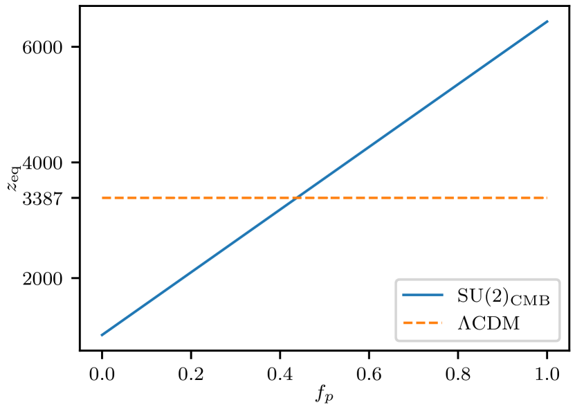
Truly matter dominated recombination is not realistic, see Fig. 2, yet this argument catches an important feature of SU(2)${}_{\textnormal{\tiny{cmb}}}$. That is, at a given redshift $z$ in some vicinity of $z_{\textnormal{\tiny{ym}},{\rm rec}}\sim 1700$ this model’s matter-density parameter $\Omega_{\textnormal{\tiny{ym}},m,0}$ in $\Omega_{\textnormal{\tiny{ym}},m}(z)=\Omega_{\textnormal{\tiny{ym}},m,0}(z+1)^{3}$ should be suppressed compared to its low-$z$ value.

When describing matter density at all $z$, the low value of $\Omega_{\textnormal{\tiny{ym}},m,0}$ in Eq. (12) is unacceptable in view of the successes of $\Lambda\text{CDM}$ as a low-$z$ model. Keeping in mind that the baryonic matter fraction of the today’s total matter content is small in $\Lambda\text{CDM}$, we posit the emergence of dark matter (edm) from a dark-energy like component in the dark sector (ds) at $z_{p}<z_{\textnormal{\tiny{ym}},{\rm rec}}$ as

$$\begin{split}\Omega_{\rm ds}(z)=\,&\Omega_{\Lambda}+\Omega_{\rm pdm,0}(z+1)^{3}+\\ &\Omega_{\rm edm,0}\left\{\begin{array}[]{lr}\left(z_{\phantom{p}}+1\right)^{3}\,,&z<z_{p}\\ \left(z_{p}+1\right)^{3}\,,&z\geq z_{p}\end{array}\right.\,.\end{split}$$ (13)

Here $\Omega_{\Lambda}$ and $\Omega_{\rm pdm,0}+\Omega_{\rm edm,0}\equiv\Omega_{\rm cdm,0}$ represent today’s density parameters for dark energy and dark matter, respectively, $\Omega_{\rm pdm,0}$ refers to primordial dark matter for all $z$ and $\Omega_{\rm edm,0}$ to emergent dark matter for $z<z_{p}$. One may question the assumption of an instantaneous release of dark matter from dark energy as described by Eq. (13). In the present work, the use of model (13) is motivated by technical simplicity. An example for such a dark sector could be an abundance of (non-topological) vortices and antivortices in a Planck-scale axion field (PSA) Adler (1969); Adler & Bardeen (1969); Bell & Jackiw (1969); Fujikawa (1979, 1980); Frieman et al. (1995); Giacosa et al. (2008), released by (non-thermal) Hagedorn transitions in the very early universe when Yang-Mills theories go confining. These vortices occur as dark energy (percolated by Kosterlitz-Thouless transitions) or as dark matter (depercolated vortex loops), the expansion of the universe converting the former to the latter. Today’s dark energy $\Omega_{\Lambda}$ could be a homogeneous-field contribution of the PSA. Lacking for the time being a detailed “microscopic” understanding of the vortex-antivortex ensemble, we here assume for simplicity only one such instantaneous depercolation to occur at $z_{p}$. The addition of an emergent component of dark matter makes the dark sector more complex. However, as argued above, an interpolation between a smaller, early-time component of dark matter to the presently observed one is required as a direct consequence of the new $T$-$z$ relation of Eq. (6). To posit a sudden transition from a dark-energy like component to the emergent dark-matter component is a simplification which may not survive the results of a detailed study of the physics of formely strongly bound vortices/antivortices in the associated percolate. It is clear though that if the mean separation between vortex/antivortex cores in the percolate is small compared to cosmological scales then the percolate does not exhibit any density contrast (like a cosmological constant). We imagine a vortex-antivortex-core interaction potential which is flat and positive for a certain range of distances but exhibits a barrier around a critical distance. To overcome this barrier energy must be released from the vortices’/antivortices’ very, gravitating field configurations after which they move independently – basically following the Hubble flow – in the sense of a pressure-free fluid. According to our present fit results, see Table 2, this transition occurs even outside of reach of future, space based gravitational-wave observatories (LISA will cover redshifts up to $z=30$). Therefore, the here-introduced complexity of the dark-sector physics is undesirable in the sense of Occam’s razor. We envisage though, that the (radiatively) predicted blackbody anomaly Hofmann (2016a), maximal for $T\sim 5\,$K, will be confirmed by terrestrial laboratory experiments. This would then strongly support the new $T$-$z$ relation (free quasi-particles) which enforces a modified dark sector similar to Eq. (13).

An important parameter of SU(2)${}_{\textnormal{\tiny{cmb}}}$ is the fraction $f_{p}$ of primordial dark matter to today’s dark matter

$$f_{p}\equiv\frac{\Omega_{\rm pdm,0}}{\Omega_{\rm pdm,0}+\Omega_{\rm edm,0}}\,.$$ (14)

Notice that in neglecting the baryonic contribution in the total matter density, Eq. (12) implies $f_{p}\approx 1/4$. In Fig. 2 the redshift of matter-radiation equality $z_{\rm eq}$ is depicted as a function of $f_{p}$. In inspecting Eq. (10) this demonstrates a certain degree of matter domination at $z_{\textnormal{\tiny{ym}},{\rm rec}}\sim 1700$ provided that $f_{p}$ is not too low.

Figure 2: The redshift of matter-radiation equality $z_{\rm eq}$ as a function of the fraction $f_{p}$ of primordial dark matter $\Omega_{\rm pdm,0}$ to today’s dark matter $\Omega_{\text{cdm,0}}=\Omega_{\rm pdm,0}+\Omega_{\rm edm,0}$ where $\Omega_{\rm edm,0}$ refers to the density parameter associated with the dark-matter portion that emerges at redshift $z_{p}<z_{\text{eq}}$ (solid line). The dashed line corresponds to $z_{\rm eq}$ in $\Lambda{\rm CDM}$.

2.1.3 The cosmological model SU(2)${}_{\textnormal{\tiny{cmb}}}$

Now we are in a position to set up the entire cosmological model SU(2)${}_{\textnormal{\tiny{cmb}}}$ in terms of its Hubble parameter $H$

$$H^{2}(z)=H_{0}^{2}\Big{(}\Omega_{\rm ds}(z)+\Omega_{b}(z)+\Omega_{{\textnormal{\tiny{ym}}}}(z)+\Omega_{\nu}(z)\Big{)}\,,$$ (15)

where $\Omega_{b}$ is the baryonic density parameter, $\Omega_{{\textnormal{\tiny{ym}}}}=\rho_{\textnormal{\tiny{ym}}}/\rho_{c}$ denotes the contribution of the SU(2) plasma, as defined in Eq. (17) below, $\rho_{c}$ is the critical density $\rho_{c}\equiv 3H_{0}^{2}/(8\pi G)$, and $\Omega_{\nu}$ refers to the neutrino density parameter. Since $\Omega_{b}$ is matter-like (cf. Eq. (11)), its $z$-dependence reads

$$\Omega_{b}=\Omega_{b,0}\left(z+1\right)^{3}\,.$$ (16)

Here, $\Omega_{b,0}$ is today’s baryonic density parameter which can be confronted with predictions from Big-Bang Nucleosynthesis (BBN) and with the results of baryon censuses. The contribution of the SU(2) plasma $\Omega_{{\textnormal{\tiny{ym}}}}$ comprises the massless mode ($\gamma$), identified with the U(1) photon, the massive quasi-particle modes ($V_{\pm}$), and the thermal ground state (gs). The sum of their energy densities reads Hofmann (2016a)

$$\rho_{\textnormal{\tiny{ym}}}=\underbrace{2\frac{T^{4}}{2\pi^{2}}\tilde{\rho}(0)}_{\equiv\rho_{\textnormal{\tiny{ym}},\gamma}}+\underbrace{6\frac{T^{4}}{2\pi^{2}}\tilde{\rho}\left(2M\right)}_{\equiv\rho_{\textnormal{\tiny{ym}},V_{\pm}}}+\underbrace{\vphantom{\frac{T^{4}}{2\pi^{2}}}4\pi\Lambda_{\textnormal{\tiny{ym}}}^{3}T}_{\equiv\rho_{\textnormal{\tiny{ym}},\text{gs}}}\,,$$ (17)

where $\tilde{\rho}$ is given as

$$\tilde{\rho}(y)=\int_{0}^{\infty}\mathrm{d}x\,x^{2}\frac{\sqrt{x^{2}+y^{2}}}{\exp\left[-\sqrt{x^{2}+y^{2}}\right]-1}\,,$$ (18)

the reduced mass $M$ reads

$$M=\frac{m_{V_{\pm}}}{2T}\,,$$ (19)

and $\Lambda_{\textnormal{\tiny{ym}}}$ denotes the Yang-Mills scale $\sim 10^{-4}$ eV Hofmann (2009). To obtain the $V_{\pm}$ mass, we demand the Legendre transformation

$$\rho_{\textnormal{\tiny{ym}}}=T\frac{\mathrm{d}P_{\textnormal{\tiny{ym}}}}{\mathrm{d}T}-P_{\textnormal{\tiny{ym}}}\,,$$ (20)

implying

$$0\overset{!}{=}\frac{\partial P_{\textnormal{\tiny{ym}}}}{\partial m_{V_{\pm}}}\,.$$ (21)

Here the pressure $P_{\textnormal{\tiny{ym}}}$ is defined as

$$P_{\textnormal{\tiny{ym}}}(\lambda,M)=-\Lambda_{\textnormal{\tiny{ym}}}^{4}\left(\frac{2\lambda^{4}}{(2\pi)^{6}}\left[2\tilde{P}(0)+6\tilde{P}(2M)\right]+2\lambda\right)\,,$$ (22)

with the dimensionless integral

$$\tilde{P}(y)=\int_{0}^{\infty}\mathrm{d}x\,x^{2}\log\left(1-\exp\left[-\sqrt{x^{2}+y^{2}}\right]\right)\,,$$ (23)

and the dimensionless temperature

$$\lambda=\frac{2\pi T}{\Lambda_{\textnormal{\tiny{ym}}}}\,.$$ (24)

Eq. (21) was solved for $m_{V_{\pm}}(T)$ in Hofmann (2016a). Note that $\Omega_{\textnormal{\tiny{ym}},\gamma}(T)=\Omega_{\textnormal{\tiny{l}},\gamma}(T)$, but that $\Omega_{\textnormal{\tiny{ym}},\gamma}(z)\neq\Omega_{\textnormal{\tiny{l}},\gamma}(z)$ because of Eq. (6). Finally, we have

$$\Omega_{\nu}(z)=\frac{7}{8}N_{\rm eff}\,\left(\frac{16}{23}\right)^{\frac{4}{3}}\Omega_{\textnormal{\tiny{ym}},\gamma}(z)\,,$$ (25)

where a modified factor for the conversion of neutrino to CMB temperature occurs because of the additional relativistic degrees of freedom during $e^{+}e^{-}$ annihilation Hofmann (2015).

2.1.4 Sound velocity $c_{s}$ and contributions to $R$

The co-moving sound horizon $r_{s}(z)$, which is a high-$z$ variable ($z\geq z_{\text{rec}}$), is given as a functional of the Hubble parameter $H(z)$ and the sound velocity $c_{s}(z)$

$$r_{s}(z)\equiv\int_{z}^{\infty}dz^{\prime}\,\frac{c_{s}(z^{\prime})}{H(z^{\prime})}\,,$$ (26)

where $c_{s}$ is represented by

$$c_{s}(z)\equiv\frac{1}{\sqrt{3(1+R(z))}}\,.$$ (27)

In $\Lambda$CDM the ratio $R_{\textnormal{\tiny{l}}}$ can be expressed in terms of entropy densities $s_{\textnormal{\tiny{l}}}$ or re-scaled energy densities $\rho_{\textnormal{\tiny{l}}}$ of baryons (b) and photons ($\gamma$),

$$R_{\textnormal{\tiny{l}}}\equiv\frac{s_{b}(z)}{s_{\textnormal{\tiny{l}},\gamma}(z)}=\frac{3}{4}\frac{\rho_{b}(z)}{\rho_{\textnormal{\tiny{l}},\gamma}(z)}\quad(z\gg 1)\,.$$ (28)

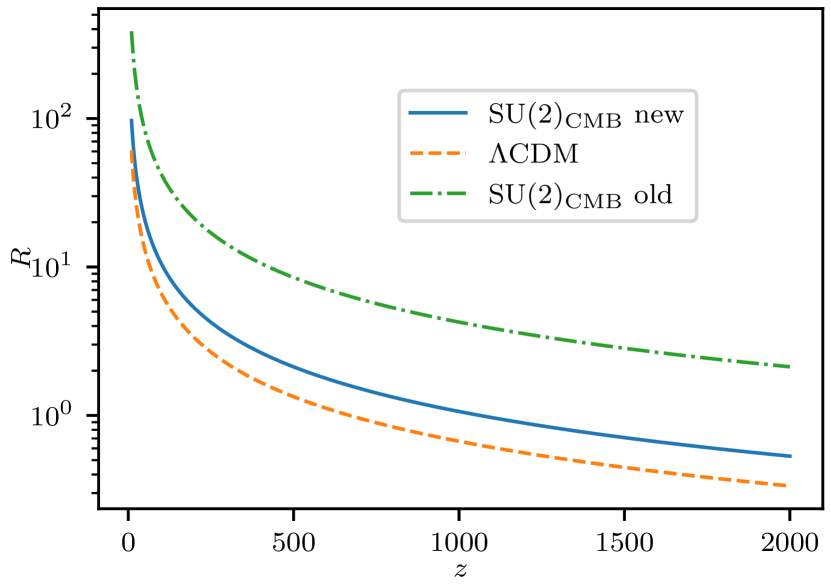
Since the entropy or energy densities in the definition of $R$ relate to conserved fluids the generalisation of Eq. (28) to the baryon-Yang-Mills plasma replaces $s_{\textnormal{\tiny{l}},\gamma}(z)$ or $\rho_{\textnormal{\tiny{l}},\gamma}(z)$ by $s_{\textnormal{\tiny{ym}}}(z)$ or $\rho_{\textnormal{\tiny{ym}}}(z)$, respectively, to define $R_{\textnormal{\tiny{ym}}}$. In Hahn & Hofmann (2017) this was overlooked. In Fig. 3 $R$ is plotted as a function of $z$ for the definition erroneously used in Hahn & Hofmann (2017), the one of the present work, which considers the full Yang-Mills plasma, and the one of $\Lambda$CDM.

Figure 3: $R$ as a function of $z$ as erroneously defined in Hahn & Hofmann (2017) (${\rm SU(2)}_{\textnormal{\tiny{cmb}}}$ old), as correctly used in the present work (${\rm SU(2)}_{\textnormal{\tiny{cmb}}}$ new), and as utilised in $\Lambda$CDM.

2.2 First order in cosmological perturbations

Eq. (15) represents the homogeneous and isotropic cosmological background. Based on this definition, we now briefly discuss the evolution of linear cosmological perturbations as induced by primordial, scalar, and adiabatic curvature perturbations. In conformal Newtonian gauge Ma & Bertschinger (1995) we consider metric perturbations subject to the line element

$$\mathrm{d}s^{2}=a(\eta)^{2}\left(-(1+2\psi)(\mathrm{d}\eta)^{2}+(1-2\phi)\mathrm{d}x^{i}\mathrm{d}x^{i}\right)\,,$$ (29)

where $\eta$ denotes the conformal time, defined by

$$\mathrm{d}\eta=\frac{\mathrm{d}t}{a}\,,$$ (30)

and $t$ is the physical time. We only consider scalar metric perturbations in terms of $\psi$ and $\phi$. The derivation of the evolution equations for $\psi$ and $\phi$ is standard Ma & Bertschinger (1995). Perturbations $\Psi$ in the phase-space distribution-functions $f$ for our relativistic degrees of freedom ($N_{\text{eff}}$ species of neutrinos, photons, and $V_{\pm}$) are governed by the first-order terms of their respective Boltzmann equations. However, we require a modified dispersion law

$$p_{\mu}p^{\mu}=m_{V_{\pm}}^{2}\,$$ (31)

where $p_{\mu}$ is the physical four-momentum, and $m_{V_{\pm}}$ denotes $V_{\pm}$’s quasi-particle mass. As a consequence of Eq. (31), $V_{\pm}$’s zeroth-order Bose-Einstein distribution function $f_{0}$ is modified compared to the massless case.

2.2.1 Initial conditions for emergent dark matter

In evolving emergent dark matter, modelled by an instantaneous depercolation of Planck-scale axion vortices at $z_{p}$, as described by Eq. (13), the according evolution equations in co-moving $k$ space,

$$\dot{\delta}_{\rm edm} = -\theta_{\rm edm}+3\dot{\phi}\,,$$

$$\dot{\theta}_{\rm edm} = -\frac{\dot{a}}{a}\theta_{\rm edm}+k^{2}\psi\,,$$ (32)

need to be supplemented with initial conditions for the density contrast ${\delta}_{\rm edm}=\frac{\delta\rho_{\rm edm}}{\rho_{\rm edm}}$ and the divergence $\theta_{\rm edm}\equiv ik^{j}v_{\text{edm},j}$ of the fluid velocity $\vec{v}_{\text{edm}}$ at conformal time $\eta_{p}$ which associates with the depercolation redshift $z_{p}$. Dots refer to differentiation w.r.t. $\eta$. In the computation of the angular power spectra we observer that strong variations,

$${\delta}_{\rm edm}(\eta_{p})=\alpha\,{\delta}_{\rm pdm}(\eta_{p})\quad(0\leq\alpha\leq 1)\,,$$ (33)

do not influence the result. On the other hand, variations in the initial condition for ${\theta}_{\rm edm}$,

$${\theta}_{\rm edm}(\eta_{p})=\beta\,{\theta}_{\rm pdm}(\eta_{p})\quad(0\leq\beta\leq 1)\,$$ (34)

influence the power at low $l$, $l\leq 30$. This conclusion is drawn from setting $\alpha=\beta=1$, minimising $\chi^{2}$ with respect to Planck’s TT, TE, and EE power spectra, and subsequently varying $\alpha$ and $\beta$ with the other cosmological parameters kept fixed. In actual fits we therefore set $\alpha=1$ and consider $\beta$ to be a free parameter.

The important feature of depercolated configurations of the Planck-scale axion field is that their individual extent (both transverse and along the vortex loop) is small on cosmological scales. Note that this may not be the case on astrophysical scales. Vortex loops (and other texture in association with the Planck-scale axion field) thus can be considered non-relativistic particles in isolation with a cosmological equation of state $P=0$. Since our simple transition of Eq. (13) from a dark-energy like component (a percolate of these field configuration) into an ideal gas of them in isolation so far only represents a parametrisation of our ignorance concerning the “microscopics” of the percolated state, including the field configurations in individual self-gravitating vortex cores, there is not yet a handle on usefully discussing causality in the initial conditions of the fluctuations in energy density and the divergence of peculiar fluid velocity in the emergent dark matter. Our initial conditions (33) and (34) assume that the according modes follow, up to a rescaling of order unity, the one of the primordial dark matter, evolved from Gaussian initial conditions throughout the linear regime. (According to Tab. 2 and Fig. 12 it is justified to assume that $z_{p}>50$). Since these exhibit zero means the fluctuations of the emergent dark matter also exhibit zero means, and energy conservation therefore is guaranteed.

2.2.2 Boltzmann hierarchy for $V_{\pm}$

We now discuss a number of points to be considered when deriving the Boltzmann hierarchy for $V_{\pm}$. Because we neglect radiative corrections in deconfining SU(2) Yang-Mills thermodynamics only the collisionless Boltzmann equation for the phase-space distribution $f$ is relevant. It reads

$$\frac{\mathrm{d}f}{\mathrm{d}\eta}=\frac{\partial f}{\partial\eta}+\frac{\mathrm{d}x^{i}}{\mathrm{d}\eta}\frac{\partial f}{\partial x^{i}}+\frac{\mathrm{d}q}{\mathrm{d}\eta}\frac{\partial f}{\partial q}+\frac{\mathrm{d}n_{i}}{\mathrm{d}\eta}\frac{\partial f}{\partial n_{i}}=0\,,$$ (35)

where the co-moving momentum $\vec{q}$ and its modulus $q$ define $\vec{n}\equiv\frac{\vec{q}}{q}$.

The only non-standard term involves the factor $\frac{\mathrm{d}q}{\mathrm{d}\eta}$. As usual, the perturbation $\Psi$ of the unperturbed phase-space distribution $f_{0}=1/(\exp(\epsilon/T_{0})-1)$ is introduced as

$$f=f_{0}(\epsilon)\left(1+\Psi\right)\,,$$ (36)

where the co-moving energy $\epsilon$ reads

$$\epsilon\equiv\left(q^{2}+a^{2}\frac{m_{V_{\pm}}^{2}}{{\cal S}^{2}\,T_{0}^{2}}\right)^{1/2}\,.$$ (37)

The scaling function $\mathcal{S}$ is defined in Eq. (5). Since the term $\frac{\mathrm{d}q}{\mathrm{d}\eta}$ is determined by the geodesic equation for a massive point particle, we may write

$$\begin{split}\frac{\mathrm{d}q}{\mathrm{d}\eta}\frac{\partial f}{\partial q}=&\left(q\dot{\phi}-\epsilon n_{i}\partial_{i}\psi-\frac{a^{2}m_{V_{\pm}}\dot{m}_{V_{\pm}}}{q}\right)\times\\ &\left(\frac{\partial f_{0}}{\partial q}(1+\Psi)+f_{0}\frac{\partial\Psi}{\partial q}\right)\,.\end{split}$$ (38)

The use of the geodesic equation for a quasi-particle must be questioned, if this particle associates with pure quantum fluctuations Hofmann (2017). If at all, temperature fluctuations in the $V_{\pm}$ sector can thus only be coherently propagated via the low-frequency regime of $\gamma$ fluctuations in terms of classical electromagnetic waves Hofmann (2016b). To do this, a residual interaction between $V_{\pm}$ and $\gamma$ is required. Albeit such an interaction occurs Hofmann (2016a), its efficiency in conveying the coherent propagation of $V_{\pm}$ temperature fluctuations must be questioned, especially at high temperatures Falquez et al. (2010). To ignore the $V_{\pm}$ Boltzmann equations and associated source terms in linearised Einstein equations thus is a physically motivated option. On the other hand, considering the evolution of $V_{\pm}$ temperature fluctuations via the coherently propagating low-frequency sector in $\gamma$ implies that $\epsilon=q$ in the $V_{\pm}$ geodesic equation. At the same time, $m_{V_{\pm}}>0$ is required in $f_{0}$. Since the structure of temperature fluctuations is mainly imprinted before and during recombination, setting $m_{V_{\pm}}=0$ in the geodesic equation does not influence the prediction for the power spectra in practice. Note that due to Eq. (37) an explicit dependence of $f_{0}$ on $\eta$ needs to be considered via $a=a(\eta)$. Transforming Eq. (35) into $k$ space and otherwise following the standard procedure of linear perturbation theory Ma & Bertschinger (1995), one arrives at the following hierarchy

$$\dot{\Psi}_{0} =-k\Psi_{1}-\frac{\mathrm{d}\ln f_{0}}{\mathrm{d}\ln q}\dot{\phi}-\frac{1+\Psi_{0}}{f_{0}}\frac{\partial f_{0}}{\partial\eta}\,,$$ (39)

$$\dot{\Psi}_{1} =\frac{k}{3}(\Psi_{0}-2\Psi_{2})-\frac{1}{3}\frac{\mathrm{d}\ln f_{0}}{\mathrm{d}\ln q}k\psi-\frac{\Psi_{1}}{f_{0}}\frac{\partial f_{0}}{\partial\eta}\,,$$ (40)

$$\dot{\Psi_{l}} =\frac{k}{(2l+1)}\left[l\Psi_{l-1}-(l+1)\Psi_{l+1}\right]-\frac{\Psi_{l}}{f_{0}}\frac{\partial f_{0}}{\partial\eta}\,,$$ (41)

where the $\Psi_{l}(\vec{k},q,\eta)$ are the expansion coefficients for $\Psi(\vec{k},\hat{n},q,\eta)$ into Legendre polynomials.

Since the $V_{\pm}$ are free quasi-particles in the here-considered approximation, their initial conditions are implemented in analogy to those of massive neutrinos Ma & Bertschinger (1995).

3 Constraints from standard ruler and $\boldsymbol{\theta_{*}}$

The angular size $\theta_{*}$ of the sound horizon $r_{s}$, see Eq. (26), at photon decoupling $z_{*}$ is defined as

$$\theta_{*}\equiv\theta(z_{*})\equiv\frac{1}{z_{*}+1}\frac{r_{s}(z_{*})}{d_{A}(z_{*})}\,,$$ (42)

where the angular diameter distance $d_{A}(z)$ reads

$$d_{A}(z)\equiv\frac{1}{z+1}\int_{0}^{z}\mathrm{d}z^{\prime}\,\frac{\mathrm{d}z^{\prime}}{H(z^{\prime})}\,.$$ (43)

Therefore, $\theta_{*}$ is an all-$z$ variable. Conventionally, $z_{*}$ denotes the redshift at which the optical depth $\tau_{*}$ is unity:

$$1\overset{!}{=}\tau_{*}(z_{*})\equiv\int_{0}^{z_{*}}\frac{\mathrm{d}z}{H(z)}\,\dot{\tau}_{*}(z)\,.$$ (44)

Here, $\dot{\tau}_{*}(z)$ is given as

$$\dot{\tau}_{*}(z)\equiv\sigma_{T}\frac{n_{e}(z)}{z+1}\,,$$ (45)

where $\sigma_{T}$ denotes the Thomson cross section, and $n_{e}$ is the number density of free electrons. Analogously, the redshift of baryon drag $z_{d}$ is conventionally obtained by replacing $\dot{\tau}_{*}(z)$ with Hu & Sugiyama (1995, 1996)

$$\dot{\tau}_{d}(z)\equiv\frac{1}{R(z)}\dot{\tau}_{*}(z)$$ (46)

in Eq. (44), where $R(z)$ is specific to the cosmological model under investigation, compare with Eq. (28) for example. In Hahn & Hofmann (2017) it was argued that due to the finite peak width in $z^{\prime}$ of the visibility function $D_{*}(z,z^{\prime})$ photon freeze-out occurs at its left flank. Function $D_{*}(z,z^{\prime})$ is given as

$$D_{*}(z,z^{\prime})\equiv\frac{\dot{\tau}_{*}(z^{\prime})}{H(z^{\prime})(z^{\prime}+1)}\exp\left(-\left[\tau_{*}(z)-\tau_{*}(z^{\prime})\right]\right)\,.$$ (47)

To determine $z_{d}$, an analogous argument relates to decoupling at the left flank of $D_{d}(z,z^{\prime})$. Notice that, with the conventional decoupling conditions, the values of $z_{*}$ and $z_{d}$ practically coincide with the peak positions of their visibility functions $D_{*}(z,z^{\prime})$ and $D_{d}(z,z^{\prime})$.

To compute $r_{d}\equiv r_{s}(z_{d})$ and $\theta_{*}$ in SU(2)${}_{\textnormal{\tiny{cmb}}}$, six parameters need to be prescribed. These are the helium fraction in baryon mass $Y_{p}$, the scaled baryon-to-photon number fraction $\eta_{10}$, $N_{\text{eff}}$, $z_{p}$, $f_{p}$, and the physical energy density

$$\omega_{\rm cdm,0}\equiv h^{2}\left(\Omega_{\rm edm,0}+\Omega_{\rm pdm,0}\right)\,,$$ (48)

where $H_{0}\equiv h\cdot 100$ km s^-1Mpc^-1. While $\theta_{*}$ is nearly model-independently and accurately determined by the observed peak structure in the TT angular power spectrum de Bernadis et al. (2000); Spergel et al. (2003); Ade et al. (2016),

$$100\cdot\theta_{*}=1.04122\pm 0.00045\,,$$ (49)

there is no such consensus about the value of the standard ruler $r_{d}$. The value of $r_{d}$ associates with a bumpy feature in the matter correlation function, introduced by baryonic acoustic oscillation (BAO) Heavens et al. (2014); Bernal, Verde & Riess (2016), and is connected to $H_{0}$ via $hr_{d}=\mbox{const}\sim 100$ Mpc Heavens et al. (2014); Bernal, Verde & Riess (2016). Our strategy in exploring the implications of SU(2)${}_{\textnormal{\tiny{cmb}}}$ is to prescribe value for $\theta_{*}$ as in Eq. (49) as well as $r_{d}$ by minimising the cost function

$$C(r_{d},\theta_{*};r_{d,o},\theta_{*,o})=\frac{\left(\theta_{*}-\theta_{*,o}\right)^{2}}{2\sigma^{2}_{*,o}}+\frac{\left(r_{d}-r_{d,o}\right)^{2}}{2\sigma^{2}_{d,o}}\,.$$ (50)

Here, $r_{d,o}$, and $\theta_{*,o}$ refer to the prescribed values, and $\sigma_{d,o}$, and $\sigma_{*,o}$ are typical errors in their observational extractions. We use $\sigma_{*,o}=0.00045/100$ (see Eq. (49)) and $\sigma_{d,o}$ as inferred from a propagated error in $H_{0}$ of $\Delta{H_{0}}\sim 1$ km s^-1Mpc^-1 Bernal, Verde & Riess (2016). Moreover, $\theta_{*,o}$ is always fixed to the value given in Eq. (49) while $r_{d,o}$ is varied in the range $135\,$Mpc$\,\leq r_{d,o}\leq 147\,$Mpc Bernal, Verde & Riess (2016). In performing the analysis, we use a Monte Carlo (MC) procedure which is inspired by the Metropolis-Hastings algorithm Metropolis et al. (1953); Hastings (1970), dubbed here MC-MH. For all of the above listed parameters of SU(2)${}_{\textnormal{\tiny{cmb}}}$ we consider the following prior ranges

$$\begin{split}0&\leq f_{p}\leq 1\,,\quad&100&\leq z_{p}\leq 900\,,\\ 5.8823&\leq\eta_{10}\leq 6.6823\,,\quad&0.2&\leq Y_{P}\leq 0.3\,,\\ 3.0&\leq N_{\text{eff}}\leq 3.2\,,\quad&0.1126&\leq\omega_{\rm cdm,0}\leq 0.1886\,.\end{split}$$ (51)

The large ranges of $f_{p}$ and $z_{p}$ are motivated by our present ignorance about the “microscopics” of Planck-scale-vortex depercolation, those of $Y_{P}$ and $\eta_{10}$ contain the BBN bounds, $N_{\text{eff}}$ is tightly constrained by particle physics on flavour neutrinos  Tanabashi et al. (2018) and neglecting sterile neutrinos. The prior range for $\omega_{\rm cdm,0}$ is bounded from below by the $\Lambda$CDM fit to the 2015 Planck data, but we allow for a generous increase as a result of our present analysis. In step $N$ and assuming uniform distributions, we compute a point in the six-dimensional parameter space spanned by  (51), calculate its values of $r_{d}$ and $\theta_{*}$, and appeal to the following decision function

$$D(r_{d},\theta_{*};r_{d,o},\theta_{*,o})=\exp\left[-C(r_{d},\theta_{*};r_{d,o},\theta_{*,o})\right]\,,$$ (52)

storing this point when the condition

$$\frac{D_{N}}{D_{N-1}}>U(0,1)$$ (53)

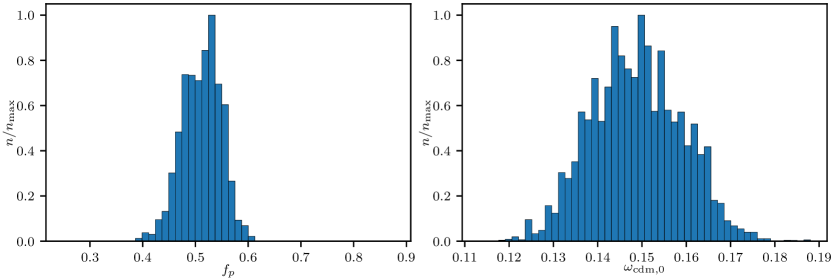
is satisfied. Here, $U(0,1)$ is a randomly generated value between zero and unity. For each parameter a histogram is thus generated from the so-obtained set of points. The histogram is composed of fifty bins within each parameter range. If a peak structure emerges, a Gaussian, whose peak position is interpreted as the preferred value, is fitted. The width of this Gaussian serves as an estimate of the error. Note that such an estimate depends on the prior ranges. Single peaks only occur for $f_{p}$ and $\omega_{\rm cdm,0}$ (see Fig. 4). For all other parameters the histograms are nearly flat. Therefore, the model determines the values of two out of its six parameters in terms of the two independent quantities $r_{d}$ and $\theta_{*}$. Our analysis may thus be restricted to the investigation of the dependencies of $f_{p}$ and $\omega_{\rm cdm,0}$ on $r_{d,o}$.

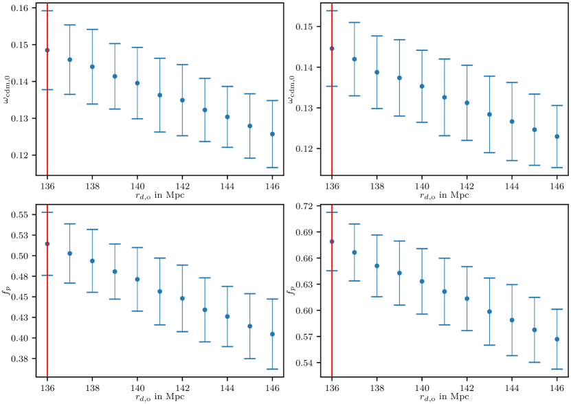
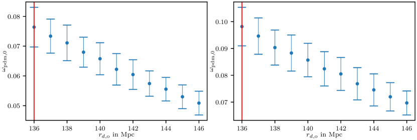
We find approximate affine dependencies on $r_{d}$ for both the conventional and left flank method discussed above, see Fig. 5. Notice that this predicts a curved function $\omega_{\rm pdm,0}=\omega_{\rm cdm,0}f_{p}$, see Fig. 6. At $r_{d,o}=136$ Mpc, which corresponds to the typical local value $H_{0}=(73.48\pm 1.66)$ km s^-1Mpc^-1 Riess et al. (2018), we obtain peak positions $\omega_{\rm pdm,0}=0.077$ (conventional) and $\omega_{\rm pdm,0}=0.098$ (left flank). From Fig. 5 we extract peak positions $\omega_{\rm cdm,0}=0.148$ (conventional) and $\omega_{\rm cdm,0}=0.144$ (left flank) at the same value of $r_{d,o}$. Compared to $\omega_{\rm cdm,0}=0.1186\pm 0.0020$ from the Planck best-fit (TT+lowP+lensing) to $\Lambda$CDM Ade et al. (2016) this is high.

Figure 4: Normalised histograms for $f_{p}$ (left panel) and $\omega_{\rm cdm,0}$ (right panel) generated from the MC-MH algorithm. We use 500000 steps and $H_{0}=73.48\,$ km s^-1Mpc^-1 Riess et al. (2018).

Figure 5: Preferred values of $\omega_{\rm cdm,0}$ (upper panels) and $f_{p}$ (lower panels) depending on the value of $r_{d,o}$ generated from the MC-MH algorithm for the conventional (left panels) and left flank (right panels) extraction method. In each case, we find affine dependencies. The vertical red line depicts the value of $r_{d,o}$ corresponding to $H_{0}=73.48\,$ km s^-1Mpc^-1  Riess et al. (2018).

Figure 6: Preferred values of $\omega_{\rm pdm,0}=\omega_{\rm cdm,0}f_{p}$ for the conventional (left panel) and left flank (right panel) extraction method, errors propagated from those of $\omega_{\rm cdm,0}$ and $f_{p}$.

4 Constraints from CMB angular power spectra

Instead of confronting SU(2)${}_{\textnormal{\tiny{cmb}}}$ with only two observationally imposed constraints, we now determine all of its parameters by means of the angular power spectra TT, TE, and EE Ade et al. (2016). To this end, we worked with the Cosmic Linear Anisotropy Solving System (CLASS)
Blas, Lesgourgues & Tram (2011) because its modular and well-documented structure allows for a targeted implementation of the modifications demanded by SU(2)${}_{\textnormal{\tiny{cmb}}}$.

4.1 Code adjustments in CLASS

Modifications are implemented in the following modules: input, background, thermodynamics, perturbation, output. Also, we have introduced an additional module unconventional.

In detail, input now contains the definitions of the additional cosmological parameters as introduced in Sec. 2.1.3: $z_{p},\,\omega_{\rm edm,0},\,\alpha,\,\beta$, and the modified conversion between neutrino temperature $T_{\nu}$ and CMB temperature $T$. The thermodynamic quantities of the SU(2) Yang-Mills plasma, see Eqs. (17) and (22), and function ${\cal S}(z)$ of Eq. (5), are computed in unconventional. In background the cosmological model is defined according to Eq. (15). We also introduce the unperturbed Bose-Einstein distribution for $V_{\pm}$ and $R_{\textnormal{\tiny{ym}}}$, the latter serving as an input in various other modules, e.g., in thermodynamics to define photon and baryon decoupling or in perturbation to define the photon-baryon scattering term in the Boltzmann equation. In thermodynamics we implement the modified $T$-$z$ relation in terms of function ${\cal S}(z)$. The Boltzmann hierarchy for $V_{\pm}$ and the Euler equation for emergent dark matter (2.2.1), including the model for the initial conditions of Eqs. (33) and (34), are now added to perturbation. The module output is extended to accommodate the additional parameters of SU(2)${}_{\textnormal{\tiny{cmb}}}$.

4.2 Best-fit results: Planck data vs. SU(2)${}_{\text{\tiny{{CMB}}}}$ and $\Lambda$CDM

To estimate effects of including/excluding the $V_{\pm}$ in the perturbation equations, see Sec. 2.2.2, we consider the following two variants of the cosmological model.
$\text{SU(2)}_{\text{\tiny{{CMB}}}}$ (physically favoured):
background model of Eq. (15), disregarding coherent temperature fluctuations as induced by the $V_{\pm}$; account for $R_{\textnormal{\tiny{ym}}}$ in all other instances.
$\text{SU(2)}_{\text{\tiny{{CMB}}}}$+$V_{\pm}$ (physically disfavoured):
background model of Eq. (15) together with participation of coherent temperature fluctuations as induced by the $V_{\pm}$ in terms of their own Boltzmann hierarchy and associated source terms in evolution of metric perturbations; account for $R_{\textnormal{\tiny{ym}}}$ in all other instances.

The utilised likelihood functions, lowTEB, HiLLiPOP, and lensing, are introduced in Aghanim et al. (2016). Omitting the lowTEB likelihood does not influence the fit results in any essential way. Prior ranges used in the fits are quoted in Tab. 1 for all free parameters. In our present investigation we fix $N_{\rm eff}$ to its central $\Lambda$CDM value: $N_{\rm eff}=3.046$. This is motivated by the observations discussed in Sec. 3.

Table 1: Prior ranges for the free parameters. Notice that fit results usually do not touch the boundaries of these ranges, see Tab. 2 and Fig. 12.

Parameter	Range
$\omega_{\text{b,0}}$	$[0.014\,\ldots\,0.027]$
$\omega_{\text{pdm,0}}$	$[0.03\,\ldots\,0.14]$
$\omega_{\text{edm,0}}$	$[0.01\,\ldots\,0.1]$
$100\,\theta_{*}$	$[0.96\,\ldots\,1.07]$
$\tau_{\text{re}}$	$[0.01\,\ldots\,0.20]$
$\ln(10^{10}\,A_{s})$	$[1.5\,\ldots\,3.2]$
$n_{s}$	$[0.4\,\ldots\,1.1]$
$z_{p}$	$[17.66\,\ldots\,2001]$
$\beta$	$[0\,\ldots\,1]$

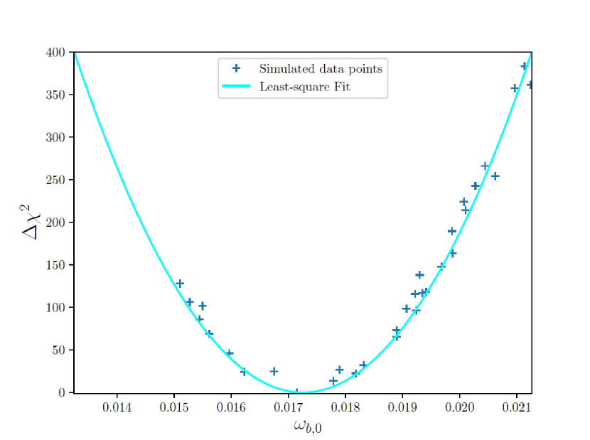
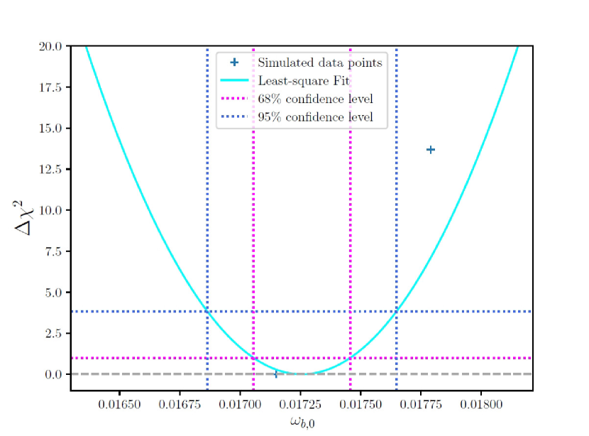
In Tab. 2 we quote our best-fit values for cosmological parameters of $\text{SU(2)}_{\textnormal{\tiny{cmb}}}$ and $\text{SU(2)}_{\textnormal{\tiny{cmb}}}$+$V_{\pm}$ in comparison with those of $\Lambda$CDM. Central values and error estimates for $\text{SU(2)}_{\textnormal{\tiny{cmb}}}$ were obtained in Kramer (2018) using profile likelihoods Henrot-Versillé et al. (2016), see Fig. 7 and Fig. 8 for further explanations.

Figure 7: Chi-square co-profile w.r.t. HiLLiPOP+lowTEB+lensing likelihood of the parameter $\omega_{\text{b,0}}$ together with the least-square fit to a parabola for $\text{SU(2)}_{\textnormal{\tiny{cmb}}}$ (left panel). Zoomed-in co-profile with intersections at $\Delta\chi^{2}=1,3.84$ corresponding to 68% and 95% confidence levels (right panel). Central value and error range (68% confidence) are quoted in the first column of Tab. 2.

Figure 8: Chi-square co-profile w.r.t. HiLLiPOP+lowTEB+lensing likelihood of the parameter $a_{p}=\frac{1}{z_{p}+1}$ together with the least-square fit to a parabola for $\text{SU(2)}_{\textnormal{\tiny{cmb}}}$ (left panel). Zoomed-in co-profile with intersections at $\Delta\chi^{2}=1,3.84$ corresponding to 68% and 95% confidence levels (right panel). Central value and error range (68% confidence) are quoted in the first column of Tab. 2.

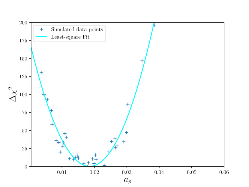
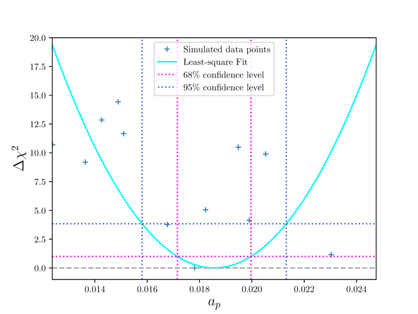
Since the co-profiling procedure is computationally expensive, only the central values were computed by brute-force minimisation in case of the (physically disfavoured) $\text{SU(2)}_{\textnormal{\tiny{cmb}}}$+$V_{\pm}$ model, no error estimates were performed.

Let us discuss the free parameters. The errors of $\omega_{\text{pdm,0}}$ and $\omega_{\text{edm,0}}$ are comparable to the error of $\omega_{\text{cdm,0}}$ in $\Lambda$CDM Kramer (2018); the typical values for $\chi^{2}/n_{\text{dof}}$ match those of $\Lambda$CDM. Judging by Fig. LABEL:fig-67-2, the co-profile for $a_{p}$ (and thus for $z_{p}$) exhibits a well discernible minimum. On the other hand, the high value of $z_{p}\sim 980$ in the case of $\text{SU(2)}_{\textnormal{\tiny{cmb}}}$+$V_{\pm}$, see Tab. 2, can be identified as an extreme outlier in spite of convergence in the brute-force MINUIT minimisation (typical local minima, obtained under variations of the starting points, cluster around values $z_{p}\sim 50$). This could be due to $\text{SU(2)}_{\textnormal{\tiny{cmb}}}$+$V_{\pm}$ unphysically propagating temperature fluctuations in the quasi-particle sector.

Notice the low values for the spectral index for primordial, scalar curvature perturbations $n_{s}$ in comparison with that of $\Lambda$CDM. The values of $\omega_{\text{b,0}}$ for both $\text{SU(2)}_{\textnormal{\tiny{cmb}}}$, $\text{SU(2)}_{\textnormal{\tiny{cmb}}}$+$V_{\pm}$ are low compared to the $\Lambda$CDM case and outside the 95% confidence level of the BBN deuterium concordance range $0.021\leq\omega_{b,0}\leq 0.024$ Patrignani et al. (2017). However, the central value for $\omega_{\text{b,0}}$, as suggested by the ⁷Li abundance, is significantly lower Patrignani et al. (2017). The value of $\omega_{\text{m,0}}$ is higher than in $\Lambda$CDM. The tendency of $\text{SU(2)}_{\textnormal{\tiny{cmb}}}$ to predict higher values of $\omega_{\text{cdm,0}}$ was already observed in the analysis of Sec. 3. For $\text{SU(2)}_{\textnormal{\tiny{cmb}}}$+$V_{\pm}$ and for $\text{SU(2)}_{\textnormal{\tiny{cmb}}}$ the values of $\omega_{\text{m,0}}$ are contained in the 68% and 95% confidence intervals for a flat universe of the SNe Ia constraints in Betoule et al. (2014), respectively. Finally, the values of $\omega_{\text{pdm,0}}$ are comparable with the one extracted with the left-flank method in Sec. 3.

The (derived) values of $H_{0}$ and $z_{\rm re}$ are in good agreement with local observation, see Riess et al. (2018) and Becker et al. (2001). Notice that $z_{d}<z_{*}$ in both $\text{SU(2)}_{\textnormal{\tiny{cmb}}}$ and $\text{SU(2)}_{\textnormal{\tiny{cmb}}}$+$V_{\pm}$ just like it is in $\Lambda$CDM.

Table 2: Best-fit cosmological parameters of the $\text{SU(2)}_{\textnormal{\tiny{cmb}}}$, $\text{SU(2)}_{\textnormal{\tiny{cmb}}}+V_{\pm}$, and the $\Lambda$CDM model. The best-fit parameters of $\Lambda$CDM together with their 68% confidence intervals are taken from Aghanim et al. (2016), employing the TT,TE,EE+lowP+lensing likelihood. For $\text{SU(2)}_{\textnormal{\tiny{cmb}}}$, $\text{SU(2)}_{\textnormal{\tiny{cmb}}}+V_{\pm}$ we use the HiLLiPOP+lowTEB+lensing likelihood as defined in Aghanim et al. (2016) (lowP and lowTEB are pixel-based likelihoods). The upper section of the table quotes free parameter values, the central section states the values of derived parameters, and the lower section the associated $\chi^{2}$ and $\chi^{2}/n_{\text{dof}}$ values for the low-$l$ ($2\leq l\leq 29$) and the high-$l$ ($30\leq l$) spectra with respective subscripts $ll$ and $hl$. Here $n_{\text{dof}}$ is defined as the difference between the number of degrees of freedom and the number of free parameters. The computations of $z_{*}$ and $z_{d}$ were performed according to the conventional criterion of Eq. (44) or its baryon-drag version. Practically, there is no dependence of other best-fit cosmological parameters on the value of $\alpha$, defined in Eq. (33), whereas this is not the case for $\beta$, defined in Eq. (34). For $\text{SU(2)}_{\textnormal{\tiny{cmb}}}$ central values are identified with the minima of co-profiles Kramer (2018). Errors correspond to 68%-confidence levels, see Fig. 7 and Fig. 8 for the cases $\omega_{\text{b,0}}$ and $a_{p}=\frac{1}{z_{p}+1}$, respectively. For the physically less motivated case of $\text{SU(2)}_{\textnormal{\tiny{cmb}}}+V_{\pm}$, see Sec. 2.2.2, we only consider the output of brute-force minimisation using MINUIT (contained in CAMEL) and refrain from performing the computationally expensive co-profiling procedure Kramer (2018). The value of $\sigma_{8}$ was only computed for $\text{SU(2)}_{\textnormal{\tiny{cmb}}}$ since its determination for $\text{SU(2)}_{\textnormal{\tiny{cmb}}}+V_{\pm}$ would have necessitated further modifications of CLASS. The central values associate with $\chi^{2}=\chi^{2}_{ll}+\chi^{2}_{hl}$ (best fit) as quoted below.

Parameter	$\text{SU(2)}_{\textnormal{\tiny{cmb}}}$	$\text{SU(2)}_{\textnormal{\tiny{cmb}}}$+$V_{\pm}$	$\Lambda$CDM
$\omega_{\text{b,0}}$	$0.0173\pm 0.0002$	0.0167	$0.0225\pm 0.00016$
$\omega_{\text{pdm,0}}$	$0.113\pm 0.002$	0.106	$-$
$\omega_{\text{edm,0}}$	$0.0771\pm 0.0012$	0.0685	$-$
$100\,\theta_{*}$	$1.0418\pm 0.0022$	1.0418	$1.0408\pm 0.00032$
$\tau_{\text{re}}$	$0.02632\pm 0.00218$	0.0166	$0.079\pm 0.017$
$\ln(10^{10}A_{s})$	$2.858\pm 0.009$	2.799	$3.094\pm 0.034$
$n_{s}$	$0.7261\pm 0.0058$	0.7022	$0.9645\pm 0.0049$
$z_{p}$	$52.88\pm 4.06$	981.45	$-$
$\beta$	$0.811\pm 0.058$	0.72	$-$
$H_{0}/$km s-1Mpc-1	$74.24\pm 1.46$	73.41	$67.27\pm 0.66$
$z_{\text{re}}$	$6.23^{+0.41}_{-0.42}$	4.41	$10^{+1.7}_{-1.5}$
$z_{*}$	$1715.19\pm 0.19$	1716.55	$1090.06\pm 0.30$
$z_{d}$	$1640.87\pm 0.27$	1639.49	$1059.65\pm 0.31$
$\omega_{\text{cdm,0}}$	$0.1901\pm 0.0023$	0.1745	$0.1198\pm 0.0015$
$\Omega_{\Lambda}$	$0.616\pm 0.006$	0.645	$0.6844\pm 0.0091$
$\Omega_{\text{m,0}}$	$0.384\pm 0.006$	0.355	$0.3156\pm 0.0091$
$\sigma_{8}$	$0.709\pm 0.020$	$-$	$0.8150\pm 0.0087$
Age$/$Gyr	$11.91\pm 0.10$	12.25	$13.799\pm 0.021$
$\chi^{2}_{ll}$	10640	10585.6	10495
$n_{\text{dof},ll}$	9207	9207	9210
$\frac{\chi^{2}_{ll}}{n_{\text{dof},ll}}$	1.156	1.150	1.140
$\chi^{2}_{hl}$	10552.6	10354.5	9951.47
$n_{\text{dof},hl}$	9547	9547	9550
$\frac{\chi^{2}_{hl}}{n_{\text{dof},hl}}$	1.105	1.085	1.042

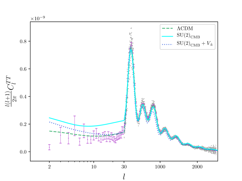
Let us now discuss the angular power spectra. In Fig. 9 the normalised spectra of the TT correlator are shown for best-fit $\text{SU(2)}_{\textnormal{\tiny{cmb}}}$, $\text{SU(2)}_{\textnormal{\tiny{cmb}}}$+$V_{\pm}$, and $\Lambda$CDM. In spite of $\chi^{2}$ being slightly smaller in $\text{SU(2)}_{\textnormal{\tiny{cmb}}}$+$V_{\pm}$ compared to $\text{SU(2)}_{\textnormal{\tiny{cmb}}}$, a visual inspection of the first three peaks suggests that the latter model fits the data better than the former one.

At low $l$ both $\text{SU(2)}_{\textnormal{\tiny{cmb}}}$ and $\text{SU(2)}_{\textnormal{\tiny{cmb}}}$+$V_{\pm}$ exhibit excesses in spectral power. This is induced by the small values of the spectral index $n_{s}$, required to fit the high-$l$ region. One should keep in mind, however, that screening effects at low $z$, neglected in the present work, break statistical isotropy and suppress the TT correlator at large angles (for a review see Hofmann (2013), for original work see Szopa & Hofmann (2008); Ludescher & Hofmann (2008)). Assuming spherical symmetry, these effects potentially account for the discrepancy between the observed and the Doppler inferred CMB dipole. Therefore, after a relaxation of this assumption, $\text{SU(2)}_{\textnormal{\tiny{cmb}}}$ induced screening is likely to substantially suppress the low-$l$ multipoles. Since the extraction of the $C_{l}$’s from a given temperature map assumes statistical isotropy, they cease to be meaningful. A quantitative assessment of a cosmological model in terms of data on the TT correlator at large angles thus requires alternative statistics Schwarz et al. (2016). We leave this complex investigation in $\text{SU(2)}_{\textnormal{\tiny{cmb}}}$ to the future.

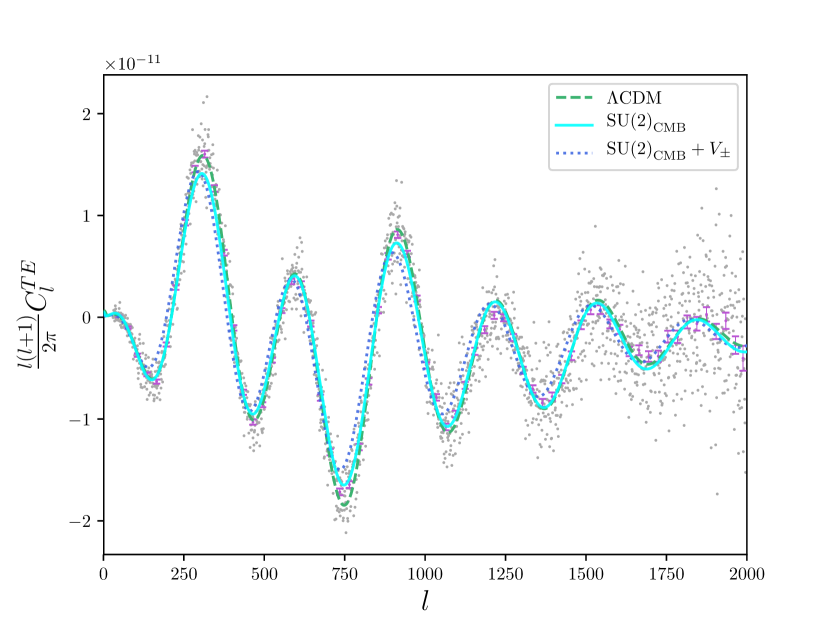
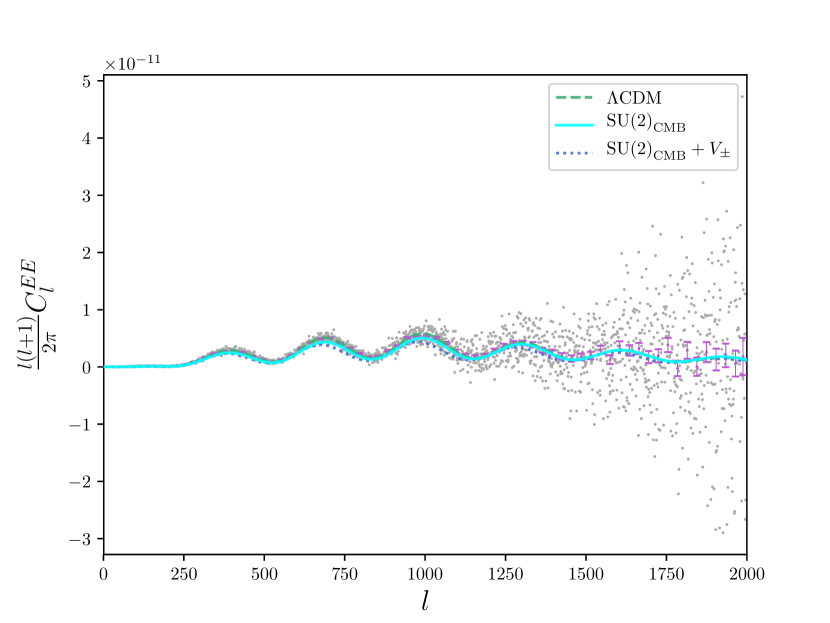
In Figs. 10 and 11 the spectra of the TE and EE cross correlators are shown: they do not differentiate the cosmological models considered and agree with the data.

Figure 9: Normalised power spectra of TT correlator for best-fit parameter values quoted in Tab. 2: Dashed, dotted, and solid lines represent $\Lambda$CDM, $\text{SU(2)}_{\textnormal{\tiny{cmb}}}$+$V_{\pm}$, and $\text{SU(2)}_{\textnormal{\tiny{cmb}}}$, respectively. For $l\leq 29$ the 2015 Planck data points are unbinned and carry error bars, for $l\geq 30$ grey points represent unbinned spectral power.

Figure 10: Normalised power spectra of TE cross correlator for best-fit parameter values quoted in Tab. 2: Dashed, dotted, and solid lines represent $\Lambda$CDM, $\text{SU(2)}_{\textnormal{\tiny{cmb}}}$+$V_{\pm}$, and $\text{SU(2)}_{\textnormal{\tiny{cmb}}}$, respectively. The 2015 Planck data points are either unbinned without error bars (grey) or binned with error bars (blue).

Figure 11: Normalised power spectra of EE cross correlator for best-fit parameter values quoted in Tab. 2: Dashed, dotted, and solid lines represent $\Lambda$CDM, $\text{SU(2)}_{\textnormal{\tiny{cmb}}}$+$V_{\pm}$, and $\text{SU(2)}_{\textnormal{\tiny{cmb}}}$, respectively. The 2015 Planck data points are either unbinned without error bars (grey) or binned with error bars (blue).

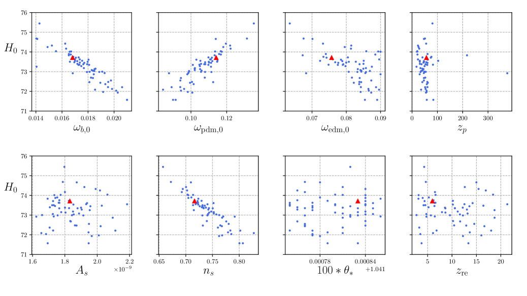
Finally, we look at the value of $H_{0}$ in dependence of all parameter values, requiring $\chi^{2}\leq 21700$, see Fig. 12. There is a conspicuous clustering around the local value of $H_{0}\sim\,73.5$ km s^-1Mpc^-1 Riess et al. (2018); Bonvin et al. (2017); there is a less pronounced clustering around the low value of $z_{\text{re}}\sim\,6$ as observed in Becker et al. (2001).

5 Summary and discussion

In the present work a cosmological model was analysed, describing a spatially flat universe and assuming the CMB to associate with an SU(2) Yang-Mills theory. The scale of this theory is fixed by the excess in line temperature at low frequencies observed by terrestrial and balloon-borne experiments, see Fixsen et al. (2011); Hofmann (2009) and references therein. Driven by an unconventional temperature-redshift relation this model requires a modified dark sector which transforms into the familiar $\Lambda$CDM model at low redshifts. With decreasing redshift, this is facilitated by an instantaneous depercolation process, characterised by the emergence of a certain amount of dark matter. The model also exhibits a neutrino sector which is subject to a modified conversion between CMB and neutrino temperatures.

In a first step, we have investigated how the constraints of the standard ruler (co-moving sound horizon at baryon drag), inferred from $H_{0}$’s local value Bernal, Verde & Riess (2016); Bonvin et al. (2017); Riess et al. (2018), and of the angular size of the sound horizon at photon decoupling fix two out of the six parameters governing the cosmological expansion. Compared to $\Lambda$CDM, we obtain a $\sim$20% excess of today’s physical total dark-matter density and a fraction of primordial to today’s total dark matter ranging from 0.5 to 0.7, subject to $H_{0}\sim 73.5\,$ km s^-1Mpc^-1 Riess et al. (2018). Other parameters of this model in addition to those introduced by linear perturbations can be determined by fits to the CMB angular power spectra TT, TE, and EE of the 2015 Planck data release Ade et al. (2016).

In a second step, we have considered two scenarios of accounting for the temperature fluctuations associated with the massive quasi-particle excitations $V_{\pm}$ in the deconfining SU(2) Yang-Mills plasma. Neglecting $V_{\pm}$ in the perturbation equations is favoured over taking them into account in view of TT data as well as theoretically Hofmann (2017). The impact of a change in scenario is negligible in the predictions of TE and EE. Presently, we have neglected any radiative, screening effects in the photon dispersion law, which play out at low redshifts and influence low multipoles, see Hofmann (2013) and references therein.

Spectra are computed with a modified version of CLASS (Cosmic Linear Anisotropy Solving System Blas, Lesgourgues & Tram (2011)). Employing typical likelihood functions of the Planck data-analysis campaign Aghanim et al. (2016) to fit these spectra, we confirm the tendency of an excess in total dark matter, and we find a red-tilted spectrum of adiabatic primordial curvature perturbations ($n_{s}\sim 0.7$) as well as low values for baryon density $\omega_{b,0}$ and reionisation depth. The low value of $n_{s}$ contradicts the standard scenario of inflationary, scale-invariant density perturbations, generated by a single slowly rolling inflaton field. In particular, our value $n_{s}\sim 0.7$ violates the slow-roll approximation, see, e.g., Wang, Mukhanov & Steinhardt (2000) and Martin & Schwarz (2000), since the leading-order term for $n_{s}$ as a function of the slow-roll parameter $\epsilon\sim 0.15$ predicts a next-to-leading order corrections of about 20%, and an expansion beyond next-to-leading order is inconsistent Wang, Mukhanov & Steinhardt (2000). One therefore would have to apply the exact method, see Wang, Mukhanov & Steinhardt (2000) and references therein, to predict the-no-longer scale invariant spectrum of adiabatic curvature perturbations from the inflaton dynamics. The epoch of inflation thus would correspond to an inflaton that appreciably rolls down its potential, implying sizable variations of the Hubble parameter.

The here-obtained excess of spectral TT power at low multipoles may reduce or completely be compensated by consideration of radiatively induced screening effects Hofmann (2013); Szopa & Hofmann (2008); Ludescher & Hofmann (2008). On the other hand, the associated breaking of statistical isotropy at low redshift casts doubts on the meaningfulness of the $C_{l}$’s at low $l$. Rather, alternative statistics should be used to unravel the physics at large angles in the CMB Schwarz et al. (2016).

There is tension of $\omega_{b,0}$ with the observed deuterium abundance, matched to the BBN prediction Patrignani et al. (2017). Presently, we interpret this as a shortcoming of our cosmological model. Yet, future reconsideration of certain assumptions in BBN together with the here-obtained low value for $\omega_{b,0}$ could contribute to a resolution of the ⁷Li puzzle. This is speculative, however, and should be solidly investigated. It is instructive, however, to compare our fit results with those of direct baryon censuses. The results discussed in Shull, Smith & Danforth (2012) suggest that baryon density mainly resides in the photoionised Lyman forest and in the warm-hot intergalactic medium (WHIM) while the collapsed phase yields a smaller correction. In total, this only amounts to about 70% of the baryons predicted by the coincidence in deuterium via BBN and the $\Lambda$CDM fit to the Planck data. (There is, however, a problem with Li.) Interestingly, this value ($0.7\times\Omega_{\rm b,0,\Lambda CDM}=0.0348$ or $0.7\times\omega_{\rm b,0,\Lambda CDM}=0.0158$) is close to our fit results (first column of Table 1): $\Omega_{\rm b,0,SU(2)_{CMB}}=0.0314$ or $\omega_{\rm b,0,SU(2)_{CMB}}=0.0173$. There is, however, a recently announced strong claim in Nicastro et al. (2018) that the missing 30% of baryons have been found in the hotter phases of WHIM by observing O VII absorbers in the X-ray spectra of quasars. These authors base their results on theoretical simulations of the hot, metal-rich filaments as well as the missing temporal structure of the signal and a missing associated cold absorption. This appears to exclude the possibility that the quasars’/blazars’ outflows or the host galaxies’ interstellar media contribute to the column densities. On the other hand, these authors declare that the sources are near the absorbing systems, and that therefore it cannot be excluded that column densities are contaminated by source outflows. To clarify the situation affirmatively, independent obervations with a clear separation of source and absorbing system should be performed. Finally, the redshift of depercolation is favoured to be 30, that is, well within the dark ages.

As for derived parameters, our best fits favour central values for $H_{0}$ in good agreement with the extractions from local cosmology Bonvin et al. (2017); Riess et al. (2016, 2018). The total matter density is about 20% higher than that of $\Lambda$CDM. Although this is at some tension with present bounds inferred from SNe Ia Hubble diagrams Betoule et al. (2014), it is not excluded. The best-fit values of the redshift $z_{\text{re}}$ for the reionisation of the universe favour the value $z_{\text{re}}\sim 6$ extracted from the Gunn-Peterson trough Becker et al. (2001).

An urgent field of research is a quantification of the screening effects for the photon, concerning a possible explanation of the suppression of the TT correlator at large angles, various power asymmetries, and the violation of Gaussianity about the CMB cold spot Schwarz et al. (2016); Hofmann (2013); Vielva (2010). Moreover, an analysis of alignments and power of the low multipoles, as induced by such screening effects, should be performed along the lines of Schwarz et al. (2016). Also, a “microscopic” understanding of the depercolation process involving the vortices of a Planck-scale axion field Frieman et al. (1995); Giacosa et al. (2008) is mandatory to validate/improve/falsify our present parametrisation of the dark sector.

References

- Abazajian et al. (2003) Abazajian K. et al., 2003, AJ, 126, 2081
- Ade et al. (2014a) Ade P. A. R. et al., 2014, A&A , 571, A1 [arXiv:1303.5062]
- Aghanim et al. (2016) Aghanim N. et al., 2016, A&A , 594, A11 [arXiv:1507.02704]
- Aghanim et al. (2016) Aghanim N. et al., 2016, A&A , 596, A107 [arXiv:1605.02985]
- Ade et al. (2016) Ade P. A. R. et al., 2016, A&A, 594, A13 [arXiv:1502.01589]
- Kramer (2018) Kramer D., 2018, “An SU(2) Yang-Mills thermal photon gas and its implications for the anisotropies in the Cosmic Microwave Background”, Master thesis, Karlsruhe Institute of Technology
- Adelman-McCarthy et al. (2008) Adelman-McCarthy J. K. et al., 2008, ApJS, 175, 297
- Adler (1969) Adler S. L., 1969, Phys. Rev., 177, 2426
- Adler & Bardeen (1969) Adler S. L., Bardeen W. A., 1969, Phys. Rev., 182, 1517
- Becker et al. (2001) Becker R. H. et al., 2001, ApJ, 122, 2850 [arXiv:astro-ph/0108097]
- Bell & Jackiw (1969) Bell J. S., Jackiw R., 1969, Nuovo Cim. A, 60, 47
- Betoule et al. (2014) Betoule M. et al., 2014, A& A, 568, A22 [arXiv:1401.4064]
- Bernal, Verde & Riess (2016) Bernal J.-L., Verde L., Riess A. G., 2016, JCAP, 10, 019 [arXiv:1607.05617]
- Blas, Lesgourgues & Tram (2011) Blas D., Lesgourgues J., Tram T., 2011, JCAP, 07, 034 [arXiv:1104.2933]
- Bonvin et al. (2017) Bonvin V. et al., 2017, MNRAS, 465, 4914 [arXiv:1607.01790]
- de Bernadis et al. (2000) de Bernardis P. et al., 2000, Nature, 404, 955 [arXiv:astro-ph/0004404]
- Cardona et al. (2017) Cardona W., Kunz M., Pettorino V., 2017, JCAP, 03, 056 [arXiv:1611.06088]
- Falquez et al. (2010) Falquez, C., Hofmann, R., Baumbach, T., 2010, Ann. d. Phys., 522, 904 [arXiv:1006.3011]
- Abbott et al. (2017) Abbott T. M. C. et al., 2017, arXiv:1711.00403
- Fixsen et al. (2011) Fixsen D. J. et al., 2011, ApJ, 734, 5 [arXiv:0901.0555]
- Frieman et al. (1995) Frieman J. A., Hill C. T., Stebbins A., Waga I., Phys. Rev. Lett., 75, 2077
- Fujikawa (1979) Fujikawa K., 1979, Phys. Rev. Lett., 42, 1195
- Fujikawa (1980) Fujikawa K., 1980, Phys. Rev. D, 21, 2848, Erratum-ibid, 1980, Phys. Rev. D, 22, 1499
- Giacosa et al. (2008) Giacosa F. et al., 2008, JHEP, 0802, 077 [arXiv:0801.0197v2]
- Hahn & Hofmann (2017) Hahn S., Hofmann R., 2017, MNRAS, 469, 1233 [arXiv:1611.02561]
- Hahn & Hofmann (2018) Hahn S., Hofmann R., 2018, Mod. Phys. Lett. A, 33, 1850029 [arXiv:1712.08561]
- Hastings (1970) Hastings W. K., 1970, Biometrika, 57, 97
- Henrot-Versillé et al. (2016) Henrot-Versillé S. et al., 2016, arXiv:1607.02964
- Hinshaw et al. (2013) Hinshaw G. F. et al., 2013, ApJ 208, 19H
- Heavens et al. (2014) Heavens, A. et al., 2014, Phys. Rev. Lett., 113, 241302 [arXiv:1409.6217]
- Hofmann (2013) Hofmann R., 2013, Nature Phys., 9, 686
- Hofmann (2009) Hofmann R., 2009, Annalen d. Physik, 18, 634 [arXiv:0902.2700]
- Hofmann (2015) Hofmann R., 2015, Annalen d. Physik, 527, 254 [arXiv:1407.1266]
- Hofmann (2016a) Hofmann R., 2016, The Thermodynamics of Quantum Yang-Mills Theory: Theory and Applications. second edition, World Scientific Publishing Co. Pte. Ltd., Singapore
- Hofmann (2016b) Hofmann, R., 2016, Entropy, 18(9), 310 [arXiv:1604.05136]
- Hofmann (2017) Hofmann, R., 2018, EPJ Web Conf. 182, 02053 [arXiv:1711.06170]
- Hu & Sugiyama (1995) Hu W., Sugiyama N., 1995, ApJ, 444, 489 [arXiv:astro-ph/9407093]
- Hu & Sugiyama (1996) Hu W., Sugiyama N., 1996, ApJ, 471, 542 [arXiv:astro-ph/9510117]
- Ludescher & Hofmann (2008) Ludescher J., Hofmann R., arXiv: 0902.3898.
- Ma & Bertschinger (1995) Ma C.-P., Bertschinger E., 1995, ApJ, 455, 7 [arXiv:astro-ph/9506072]
- Marra et al. (2013) Marra V., 2013, Phys. Rev. Lett., 110, 241305 [arXiv:1303.3121]
- Martin & Schwarz (2000) Martin J., Schwarz D. J., 2000, Phys. Rev D., 62, 103520 [arXiv:astro-ph/991122]
- Mather et al. (1990) Mather J. C. et al., 1990, ApJ, 354, L37
- Metropolis et al. (1953) Metropolis N. et al., 1953, J. Chem. Phys., 21, 1087
- Wang, Mukhanov & Steinhardt (2000) Wang L., Mukhanov V. F., Steinhardt P. J., 1997, Phys. Lett. B, 414, 18 [arXiv:astro-ph/9709032]
- Nicastro et al. (2018) Nicastro F. et al., 2018, Nature, 558, 406 [arXiv:1806.08395]
- Odderskov, Hannestad & Haugbølle (2014) Odderskov I., Hannestad S., Haugbølle T., 2014, JCAP, 10, 028 [arXiv:1407.7364]
- Odderskov, Hannestad & Brandbyge (2017) Odderskov I., Hannestad S., Brandbyge J., 2017, JCAP, 3, 022 [arXiv:1701.05391]
- Perlmutter et al. (1998) Perlmutter S. et al., 1998, ApJ, 517, 565
- Riess et al. (1998) Riess A. et al., 1998, AJ, 116, 1009
- Riess et al. (2016) Riess A. G. et al., 2016, ApJ, 826, 56 [arXiv:1604.01424]
- Riess et al. (2018) Riess A. G. et al., 2018, ApJ, 855, 136 [arXiv:1801.01120]
- Schwarz et al. (2016) Schwarz D. J., 2016, Class. Quant. Grav, 33, 184001 [arXiv:1510.07929]
- Shull, Smith & Danforth (2012) Shull J. M., Smith B. D., Danforth C. W., 2012, ApJ, 759, 23 [arXiv:1112.2706]
- Spergel et al. (2003) Spergel D. N. et al., 2003, ApJS, 148, 175 [arXiv:astro-ph/0302209]
- Szopa & Hofmann (2008) Szopa M., Hofmann R., 2008, JCAP, 0803, 0001 [arXiv:hep-ph/0703119]
- Tanabashi et al. (2018) Tanabashi M. et al. (Particle Data Group), 2018, Phys. Rev. D, 98, 010001
- Patrignani et al. (2017) Patrignani C. et al. (Particle Data Group), 2017, Chin. Phys. C, 40, 100001
- Vielva (2010) Vielva P., 2010, Adv. Astron., 2010, 592094 [arXiv:1008.3051]
- Wu & Huterer (2017) Wu H., Huterer D., 2017, MNRAS, 471, 4946 [arXiv:1706.09723]