Open-Flavour Mesons from the Angle of
Bethe, Dyson, Salpeter, Schwinger, et al.

Abstract:

Recently, we completed a comprehensive investigation of a huge part of the entire meson spectrum by considering both quarkonia and open-flavour mesons by means of a single common framework which unites the homogeneous Bethe–Salpeter equation that describes mesons as quark–antiquark bound states and the Dyson–Schwinger equation that governs the full quark propagator: Adopting two (as a matter of fact, not extremely diverse) models that attempt to grasp all principal aspects of the effective strong interactions entering identically in both these equations, we derived within this unique setup, for all mesons analysed, their masses and leptonic decay constants as well as, for the pseudoscalar ones among these mesons, their in-hadron condensates. Here, as a kind of promotion or teaser, we give but a few examples of the resulting collections of data, laying the main emphasis on the dependence of our insights on the effective-interaction model underlying all such outcomes.

1 Aim: Unique Poincaré-Covariant Study of Quarkonia and Open-Flavour Mesons

So far, Poincaré-covariant meson studies do not treat bound states of quark and antiquark of the same type (quarkonia) and of two unequal types (open-flavour mesons) by a single setup. In order to connect the two sides of the same coin, we embark on a comprehensive analysis of the whole meson spectrum by applying exactly identical Poincaré-covariant descriptions to all possible combinations of quark flavour [1, 2]. Specifically, for each meson bound state $(\bar{q}\,q^{\prime})$ of momentum $P,$ composed of antiquark $\bar{q}$ and quark $q^{\prime},$ we derive both mass $M_{\bar{q}\,q^{\prime}}$ and leptonic decay constant $f_{\bar{q}\,q^{\prime}}$ defined, e.g., by

$$\langle 0|\!:\!\bar{q}^{\prime}(0)\,\gamma_{\mu}\,\gamma_{5}\,q(0)\!:\!|(\bar{q}\,q^{\prime})(P)\rangle={\rm i}\,f_{\bar{q}\,q^{\prime}}\,P_{\mu}\qquad\mbox{for the pseudoscalar mesons}\ .$$

2 Merger: Quark Dyson–Schwinger Equation and Meson Bethe–Salpeter Equation

Trusting in quantum field theory, we adopt for the global study of quark–antiquark bound states the well-established Bethe–Salpeter approach augmented by the quark Dyson–Schwinger equation. The fact that any such equation belongs to an infinite tower of coupled Dyson–Schwinger equations renders the truncation of the tower inevitable. All not available impact (hence dubbed unobtainium) of thereby skipped relations on the retained ones has to be mimicked by, e.g., sophisticated ansatzes.

Crucial ingredients to any such approach are, for two bound-state constituents discriminated by a subscript $i=1,2,$ their dressed propagators $S_{i}(p),$ deducible as solutions of the Dyson–Schwinger equation for the corresponding two-point Green function. In rainbow truncation and if Pauli–Villars regularized at a scale $\Lambda,$ the Dyson–Schwinger equation for the dressed quark propagator $S(p)$ reads

$$S^{-1}(p)=Z_{2}\,({\rm i}\,\gamma\cdot p+m_{\rm b})+\frac{4}{3}\,Z_{2}^{2}\!\int^{\Lambda}\frac{{\rm d}^{4}q}{(2\pi)^{4}}\,{\mathcal{G}}\!\left((p-q)^{2}\right)T_{\mu\nu}(p-q)\,\gamma_{\mu}\,S(q)\,\gamma_{\nu}\ ,$$ (1)

involving the quark wave-function renormalization constant $Z_{2}$, the bare quark mass $m_{\rm b}$ related by a mass renormalization constant $Z_{m}$ to the running quark mass $m_{q}(\mu)$ renormalized at a given scale $\mu$,

$$m_{\rm b}=Z_{m}\,m_{q}(\mu)\ ,$$

the transverse projection operator $T_{\mu\nu}(k)$ as a relic of the free gluon propagator in the Landau gauge,

$$T_{\mu\nu}(k)\equiv\delta_{\mu\nu}-\frac{k_{\mu}\,k_{\nu}}{k^{2}}\ ,$$

and an effective interaction ${\mathcal{G}}(k^{2}),$ constructed such as to encompass (the bulk of) the effects of both full gluon propagator and full quark–gluon vertex entering in the quark Dyson–Schwinger equation.

The Bethe–Salpeter formalism encodes a two-fermion bound state of relative momentum $p$ and total momentum $P$ by either the Bethe–Salpeter wave function $\chi(p;P),$ defined as Fourier transform of the matrix element of the time-ordered product of these fermion fields evaluated between vacuum and bound state, or the Bethe–Salpeter amplitude $\Gamma(p;P),$ differing by the two fermion propagators:

$$\chi(p;P)\equiv S_{1}(p+\eta\,P)\,\Gamma(p;P)\,S_{2}(p-(1-\eta)\,P)\ ,\qquad\eta\in[0,1]\ .$$

Both manifestations of bound states are solutions of one and the same homogeneous Bethe–Salpeter equation. In rainbow–ladder truncation, the quark–antiquark Bethe–Salpeter equation is of the form

$$\Gamma(p;P)=-\frac{4}{3}\,Z_{2}^{2}\!\int^{\Lambda}\frac{{\rm d}^{4}q}{(2\pi)^{4}}\,{\mathcal{G}}\!\left((p-q)^{2}\right)T_{\mu\nu}(p-q)\,\gamma_{\mu}\,\chi(q;P)\,\gamma_{\nu}\ .$$ (2)

Chiral symmetries are properly embedded if the effective coupling ${\mathcal{G}}(k^{2})$ is the same as in Eq. (1).

3 Exemplification: Masses, Leptonic Decay Constants, and In-Hadron Condensates

In modelling the effective interaction in Eqs. (1,2), we follow two closely related strategies:

• Ref. [3] tries to capture also the genuine ultraviolet behaviour of the coupling function ${\mathcal{G}}(k^{2});$

• Ref. [4] is content with an easier-to-handle simpler behaviour of the coupling function ${\mathcal{G}}(k^{2}).$

Employing more than just a single model for the effective couplings enables the estimate of, at least, part of the systematic uncertainties accompanying the findings of the framework sketched in Sect. 2.

Meson quark–antiquark bound states carrying total spin $s=0,1$ and orbital angular momentum $\ell=0,1,2,\dots$ can be classified, with respect to their total angular momentum $J,$ parity $P=(-1)^{\ell+1},$ and (only where applicable) charge-conjugation parity $C=(-1)^{\ell+s},$ in terms of the designations [2]

ordinary: $$J^{P\,C}\in\{0^{++},0^{-+},1^{++},1^{+-},1^{--},2^{++},2^{-+},2^{--},3^{++},3^{+-},3^{--},4^{++},4^{-+},4^{--},\ldots\}\ ,$$

exotic: $$J^{P\,C}\in\{0^{+-},0^{--},1^{-+},2^{+-},3^{-+},4^{+-},5^{-+},\ldots\}\ .$$

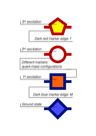
Figure 1: Legend to Figs. 2 through 4: in our system, the marker related to some meson bound state identifies the respective meson features by the colour of its edge (blue for mass and red for leptonic decay constant), the levels of excitation by the colour of its fill (blue, orange, white, yellow, …, in increasing order), and the quark combinations in our various evaluations of the quark masses by its shape (diamond, square, circle, pentagon). Horizontal blue lines delimit the accessible meson-mass ranges originating in the appearance of singularities.

Covering the full mass range from a fictitious massless quark labelled $\chi$ up to the bottom quark, we organize our findings for masses and leptonic decay constants of meson ground states and lowest radial excitations [1, 2] in plots for spin, parity, and charge-conjugation parity combinations $J^{P\,(C)}$ as shown for the strange and charmed, strange mesons in Figs. 2 and 3, and for the charmonia in Fig. 4.

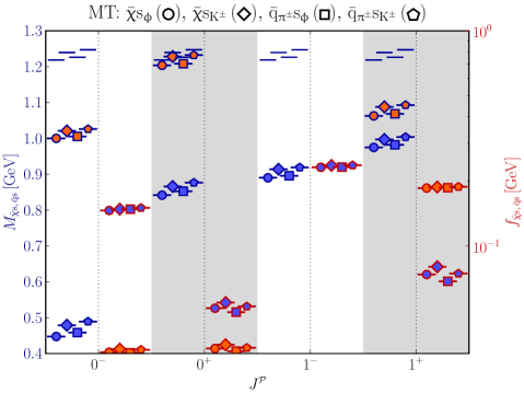
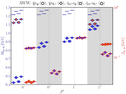
Figure 2: Strange mesons [1, Figs. 14 and 5]: Masses $M_{\bar{\chi}s,\bar{q}s}$ (left) and leptonic decay constants $f_{\bar{\chi}s,\bar{q}s}$ (right), from the ${\mathcal{G}}(k^{2})$ couplings of Refs. [3] (top) and [4] (bottom). Note, e.g., an additional $0^{+}$ excitation in the top.

Combining, for confrontation with experiment, the results of the adopted effective-coupling models (see, e.g., Fig. 5), we find an unexpectedly large model dependence, manifesting even in the number of accessible states (i.e., not only in numerical meson properties): the interaction of Ref. [3] tends to provide more states. Our complete set of predictions can be found, also in form of tables, in Ref. [1].

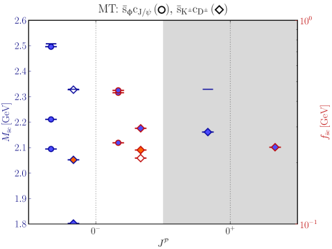
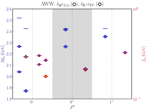
Figure 3: Charmed, strange mesons [1, Figs. 17 and 8]: Masses $M_{\bar{s}c}$ (left) and decay constants $f_{\bar{s}c}$ (right), due to the ${\mathcal{G}}(k^{2})$ ansätze of Refs. [3] (top) and [4] (bottom). Note the $1^{+}$ state in the bottom, not present in the top.

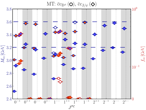
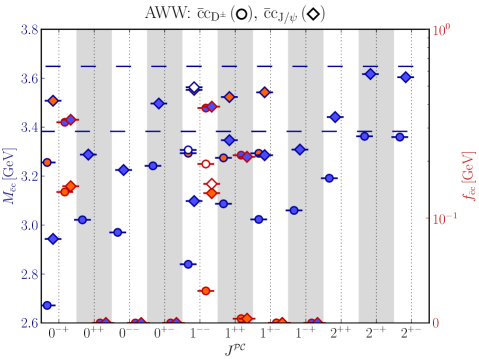
Figure 4: Charmonium [1, Figs. 18 and 9]: Masses $M_{\bar{c}c}$ (left) and decay constants $f_{\bar{c}c}$ (right), arising from the ${\mathcal{G}}(k^{2})$ models of Refs. [3] (top) and [4] (bottom). The top results reveal many more ground and excited states.

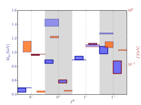
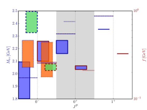
Figure 5: Mass spectra and leptonic decay constants of strange and charmed, strange mesons [1, Figs. 24 and 25]: combined results using both ${\mathcal{G}}(k^{2})$ models (narrow boxes) confronted with experiment [5] (wide boxes).

Last, but not least, Fig. 6 presents the numerical values of the in-hadron condensate, referred to as $\langle\bar{q}\,q\rangle$ [6]. The latter quantity is defined, for some pseudoscalar meson $(\bar{q}\,q^{\prime}),$ by the product of this state’s leptonic decay constant $f_{\bar{q}\,q^{\prime}}$ and projection onto an interpolating quark-bilinear pseudoscalar operator $\bar{q}^{\prime}\,\gamma_{5}\,q$ and satisfies a generalization of the good old Gell-Mann–Oakes–Renner relation [6].

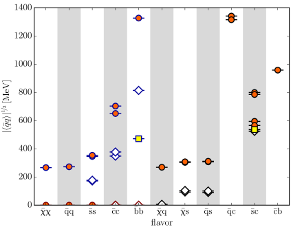
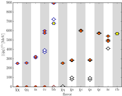
Figure 6: In-meson condensates [1, Figs. 21 and 12] for the ${\mathcal{G}}(k^{2})$ ansätze of Refs. [3] (top) and [4] (bottom).

References

- [1] T. Hilger, M. Gómez-Rocha, A. Krassnigg, and W. Lucha, Eur. Phys. J. A 53 (2017) 213, arXiv:1702. 06262 [hep-ph].
- [2] T. Hilger, M. Gómez-Rocha, A. Krassnigg, and W. Lucha, preprint HEPHY-PUB 1003/18 (2018), arXiv:1807.06245 [hep-ph].
- [3] P. Maris and P. C. Tandy, Phys. Rev. C 60 (1999) 055214, arXiv:nucl-th/9905056.
- [4] R. Alkofer, P. Watson, and H. Weigel, Phys. Rev. D 65 (2002) 094026, arXiv:hep-ph/0202053.
- [5] Particle Data Group (M. Tanabashi et al.), Phys. Rev. D 98 (2018) 030001.
- [6] P. Maris, C. D. Roberts, and P. C. Tandy, Phys. Lett. B 420 (1998) 267, arXiv:nucl-th/9707003.