\stackMath

Learning-based physical layer communications for multi-agent collaboration

Arsham Mostaani$\,{}^{1}$, Osvaldo Simeone$\,{}^{2}$, Symeon Chatzinotas$\,{}^{1}$ and Bjorn Ottersten$\,{}^{1}$ 1 SIGCOM laboratory, SnT Interdisciplinary Centre,
University of Luxembourg, Luxembourg
2 Centre for Telecom. Research, Department of Informatics,
Kingโ€™s College London, London, UK
{arsham.mostaani,symeon.chatzinotas,bjorn.ottersten}@uni.lu , {osvaldo.simeone}@kcl.ac.uk
Abstract

Consider a collaborative task carried out by two autonomous agents that can communicate over a noisy channel. Each agent is only aware of its own state, while the accomplishment of the task depends on the value of the joint state of both agents. As an example, both agents must simultaneously reach a certain location of the environment, while only being aware of their own positions. Assuming the presence of feedback in the form of a common reward to the agents, a conventional approach would apply separately: (i) an off-the-shelf coding and decoding scheme in order to enhance the reliability of the communication of the state of one agent to the other; and (ii) a standard multi-agent reinforcement learning strategy to learn how to act in the resulting environment. In this work, it is argued that the performance of the collaborative task can be improved if the agents learn how to jointly communicate and act. In particular, numerical results for a baseline grid world example demonstrate that the jointly learned policy carries out compression and unequal error protection by leveraging information about the action policy.

Index Terms:
Reinforcement learning, communication theory, unequal error protection, machine learning for communication, multi-agent systems

I Introduction

Consider the rendezvous problem illustrated in Fig. 1 and Fig. 2. Two agents, e.g., members of a SWAT team, need to arrive at the goal point in a grid world at precisely the same time, while starting from arbitrary positions. Each agent only knows its own position but is allowed to communicate with the other agent over a noisy channel. This set-up is an example of cooperative multiple agent problems in which each agent has partial information about the environment [1, 2]. In this scenario, communication and coordination are essential in order to achieve the common goal [3, 4, 5], and it is not optimal to design the communication and control strategies separately [5, 6].

Refer to caption
Figure 1: An illustration of the cooperative multi-agent system.
Refer to caption
Figure 2: The rendezvous problem: (a) illustration of the environment state-space, $\mathcal{S}^{e}$, i.e., the location on the grid, of the environment action space $\mathcal{A}^{e}$, denoted by arrows, and of the goal state, marked with gray background; (b) demonstration of a sampled episode, where arrows show the environment actions taken by the agents (empty arrows: actions of agent 1, solid arrows: actions of agent 2) and the $B=4$ bits represent the message sent by each agent. A larger reward $R_{2}>R_{1}$ is given to both agents when they enter the goal point at the same time, as in the example; (c) in contrast, $R_{1}$ is the reward accrued by agents when only one agent enters the goal position.

Assuming the presence of a delayed and sparse common feedback signal that encodes the team reward, cooperative multi-agent problems can be formulated in the framework of multi-agent reinforcement learning. As attested by the references [1, 2, 7] mentioned above, as well by [8, 9], this is a well-studied and active field of research. To overview some more recent contributions, paper [10] presents simulation results for a distributed tabular Q-learning scheme with instantaneous communication. Deep learning approximation methods are applied in [11] for Q-learning and in [12] for actor-critic methods. In [13], a method is proposed that keeps a centralized critic in the form of a Q-function during the learning phase and uses a counter-factual approach to carry out credit assignment for the policy gradients.

The works mentioned above assume a noiseless communication channel between agents or use noise as a form of regularization [9]. In contrast, in this paper, we consider the problems of simultaneously learning how to communicate on a noisy channel and how to act, creating a bridge between the emerging literature on machine learning for communications [14] and multi-agent reinforcement learning.

Our specific contributions are as follows. First, we formulate distributed Q-learning algorithms that learn simultaneously what to communicate on a noisy channel and which actions to take in the environment in the presence of communication delays. Second, for the rendezvous problem illustrated in Fig. 2, we provide a numerical performance comparison between the proposed multi-agent reinforcement learning scheme and a conventional method. The proposed scheme jointly learns how to act and communicate, where the conventional method applies separately an off-the-shelf channel coding scheme for communication and multi-agent reinforcement learning to adopt the action policies. Unlike the conventional method, the jointly optimized policy is seen to be able to learn a communication scheme that carries out data compression and unequal error protection as a function of the action policy.

II Problem Set-up

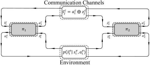
As illustrated in Fig. 1 and Fig. 2, we consider a cooperative multi-agent system comprising of two agents that communicate over noisy channels. The system operates in discrete time, with agents taking actions and communicating in each time step $t=1,2,...$. While the approach can be applied more generally, in order to fix the ideas, we focus here on the rendezvous problem illustrated in Fig. 2. The two agents operate on an $n\times n$ grid world and aim at arriving at the same time at the goal point on the grid. The position of each agent $i\in\{1,2\}$ on the grid determines its environment state sieโˆˆ๐’ฎe=[n]ร—[n]subscriptsuperscript๐‘ ๐‘’๐‘–superscript๐’ฎ๐‘’delimited-[]๐‘›delimited-[]๐‘›s^{e}_{i}\in\mathcal{S}^{e}=[n]\times[n], where $[n]=\{1,2,...,n\}$. Each agent $i$th environment state sieโˆˆ๐’ฎesubscriptsuperscript๐‘ ๐‘’๐‘–superscript๐’ฎ๐‘’s^{e}_{i}\in\mathcal{S}^{e} can also be written as the pair sie=โŸจsi,xe,si,yeโŸฉsubscriptsuperscript๐‘ ๐‘’๐‘–subscriptsuperscript๐‘ ๐‘’๐‘–๐‘ฅsubscriptsuperscript๐‘ ๐‘’๐‘–๐‘ฆs^{e}_{i}=\langle s^{e}_{i,x},s^{e}_{i,y}\rangle, with si,xe,si,yeโˆˆ[n]subscriptsuperscript๐‘ ๐‘’๐‘–๐‘ฅsubscriptsuperscript๐‘ ๐‘’๐‘–๐‘ฆdelimited-[]๐‘›s^{e}_{i,x}\,,s^{e}_{i,y}\in[n] being respectively the horizontal and vertical coordinates. Each episode terminates as soon as an agent or both visit the goal point which is denoted as ๐’ฎTe={sTe}subscriptsuperscript๐’ฎ๐‘’๐‘‡subscriptsuperscript๐‘ ๐‘’๐‘‡\mathcal{S}^{e}_{T}=\{s^{e}_{T}\}. At time $t=1$, the initial position $\mathrm{s}_{i,t=1}^{e}$, is randomly and uniformly selected amongst the non-goal states. Note that, throughout, we use Roman font to indicate random variables and the corresponding standard font for their realizations.

At any time step $t=1,2,...$ each agent $i$ has information about its position, or environment state, si,tesubscriptsuperscript๐‘ ๐‘’๐‘–๐‘กs^{e}_{i,t} and about the signal si,tcsubscriptsuperscript๐‘ ๐‘๐‘–๐‘กs^{c}_{i,t} received from the other agent jโ‰ i๐‘—๐‘–j\neq{i} at the previous time step $t-1$. Based on this information, agent $i$ selects its environment action $a_{i}^{e}=\langle a^{e}_{i,x},a^{e}_{i,y}\rangle$ from the set $\mathcal{A}^{e}=\{\langle 1,0\rangle,\langle-1,0\rangle,\langle 0,0\rangle,\langle 0,1\rangle,\langle 0,-1\rangle\}$, where $a^{e}_{i,x}$ and $a^{e}_{i,y}$ represent the horizontal and vertical move of agent $i$ on the grid. Furthermore, it chooses the communication message to send to the other agent by selecting a communication action $a^{c}_{i}\in\mathcal{A}^{c}=\{0,1\}^{B}$ of $B$ bits.

The environment state transition probability for agent $i$ can be described by the equation $\mathrm{s}^{e}_{i,t+1}=\mathrm{s}^{e}_{i,t}+\mathrm{a}^{e}_{i,t}\,$, with the caveat that, if an agent on an edge of the grid world selects an action that transfers it out, the environment keeps the agent at its current location. Agents communicate over interference-free channels using binary signaling, and the channels between the two agents are independent Binary Symmetric Channels (BSCs), such that the received signal is given as

$$\mathrm{s}^{c}_{j,t+1}={a}^{c}_{i,t}\oplus\mathrm{z}^{c}_{j,t},$$ (1)

where the XOR operation $\oplus$ is applied element-wise, and $\mathrm{z}^{c}_{j,t}$ has independent identically distributed (i.i.d.) Bernoulli entries with bit flipping probability $q\leq 0.5$.

Each agent $i$ follows a policy $\pi_{i}$ that maps the observations si=โŸจsie,sicโŸฉsubscript๐‘ ๐‘–subscriptsuperscript๐‘ ๐‘’๐‘–subscriptsuperscript๐‘ ๐‘๐‘–s_{i}=\langle s^{e}_{i},s^{c}_{i}\rangle of the agent into its actions $a_{i}=\langle a^{e}_{i},a^{c}_{i}\rangle$. The policy is generally stochastic, and we write it as the conditional probability ฯ€iโ€‹(ai|si)subscript๐œ‹๐‘–conditionalsubscript๐‘Ž๐‘–subscript๐‘ ๐‘–\pi_{i}(a_{i}|s_{i}) of taking action $a_{i}$ while in state sisubscript๐‘ ๐‘–s_{i}. We assume the policy $\pi_{i}$ to be factorized as

ฯ€iโ€‹(ai|si)=ฯ€ieโ€‹(aie|sie,sic)โ€‹ฯ€icโ€‹(aic|sie),subscript๐œ‹๐‘–conditionalsubscript๐‘Ž๐‘–subscript๐‘ ๐‘–superscriptsubscript๐œ‹๐‘–๐‘’conditionalsuperscriptsubscript๐‘Ž๐‘–๐‘’superscriptsubscript๐‘ ๐‘–๐‘’superscriptsubscript๐‘ ๐‘–๐‘superscriptsubscript๐œ‹๐‘–๐‘conditionalsuperscriptsubscript๐‘Ž๐‘–๐‘superscriptsubscript๐‘ ๐‘–๐‘’\pi_{i}(a_{i}|s_{i})=\pi_{i}^{e}(a_{i}^{e}|s_{i}^{e},s_{i}^{c})\,\pi_{i}^{c}(a_{i}^{c}|s_{i}^{e}), (2)

into a component selecting the environment action $a^{e}_{i}$ based on the overall state sisubscript๐‘ ๐‘–s_{i} and one selecting the transmitted signal $a^{c}_{i}$ based on the current position siesubscriptsuperscript๐‘ ๐‘’๐‘–s^{e}_{i}. The overall joint policy $\pi$ is given by the product $\pi=\pi_{1}\times\pi_{2}$. It is noted that the assumed memoryless stationary policies are sub-optimal under partial individual observability of environment state [1].

At each time $t$, given states โŸจs1,s2โŸฉsubscript๐‘ 1subscript๐‘ 2\langle s_{1},s_{2}\rangle and actions $\langle a_{1},a_{2}\rangle$, both agents receive a single team reward

rt={R1,ifย sieโ‰ sjeโˆˆ๐’ฎTeR2,ifย sie=sjeโˆˆ๐’ฎTe,0,otherwise,subscriptr๐‘กcasessubscript๐‘…1ifย sieโ‰ sjeโˆˆ๐’ฎTesubscript๐‘…2ifย sie=sjeโˆˆ๐’ฎTe0otherwise\mathrm{r}_{t}=\begin{cases}R_{1},&\text{if ${s}^{e}_{i}\neq{s}^{e}_{j}\in\mathcal{S}_{T}^{e}$}\\ R_{2},&\text{if ${s}^{e}_{i}={s}^{e}_{j}\in\mathcal{S}_{T}^{e}$},\\ 0,&\text{otherwise},\\ \end{cases} (3)

where $R_{1}<R_{2}$. Accordingly, when only one agent arrives at the target point sTesubscriptsuperscript๐‘ ๐‘’๐‘‡s^{e}_{T}, a smaller reward $R_{1}$ is obtained at the end of the episode, while the larger reward $R_{2}$ is attained when both agents visit the goal point at the same time. The goal of the multi-agent system is to find a joint policy $\pi$ that maximizes the expected return. For given initial states, (s1,t=1,s2,t=1)subscript๐‘ 1๐‘ก1subscript๐‘ 2๐‘ก1({s}_{1,t=1},s_{2,t=1}), this amounts to solving the problem

maximize๐œ‹๐”ผฯ€โ€‹[Gt|s1,t=1=s1,t=1,s2,t=1=s2,t=1],๐œ‹maximizesubscript๐”ผ๐œ‹delimited-[]formulae-sequenceconditionalsubscriptG๐‘กsubscripts1๐‘ก1subscript๐‘ 1๐‘ก1subscripts2๐‘ก1subscript๐‘ 2๐‘ก1\displaystyle\underset{\pi}{\text{maximize}}\quad\quad{\mathbb{E}_{\pi}[\mathrm{G}_{t}|\mathrm{s}_{1,t=1}={s}_{1,t=1},\mathrm{s}_{2,t=1}=s_{2,t=1}]},\quad (4)

where

$$\mathrm{G}_{t}=\sum_{t=1}^{\infty}\gamma^{t}\mathrm{r}_{t}\quad$$ (5)

is the long-term discounted return, with $\gamma\in(0,1]$ being the reward discount factor. The expected return in (4) is calculated with respect to the probability of the trace of states, actions, and rewards induced by the policy $\pi$ [15].

III Learned Communication

In this section we consider a strategy that jointly learns the communication and the environment action policies of both agents, by tackling problem (4). To this end, we apply the policy decomposition (2) and use the distributed Q-learning algorithm [5]. Accordingly, given the received communication signal sicsubscriptsuperscript๐‘ ๐‘๐‘–s^{c}_{i} and the local environment state siesubscriptsuperscript๐‘ ๐‘’๐‘–s^{e}_{i}, each agent $i$ selects its environment actions $a^{e}_{i}$ by following a policy $\pi^{e}_{i}$ based on a state-action value function Qieโ€‹(sie,sic,aie)subscriptsuperscript๐‘„๐‘’๐‘–subscriptsuperscript๐‘ ๐‘’๐‘–subscriptsuperscript๐‘ ๐‘๐‘–subscriptsuperscript๐‘Ž๐‘’๐‘–Q^{e}_{i}(s^{e}_{i},s^{c}_{i},a^{e}_{i}); and it chooses its communication action $a^{c}_{i}$ by following a second policy $\pi^{c}_{i}$, based on a state-action function Qicโ€‹(sie,aic)subscriptsuperscript๐‘„๐‘๐‘–subscriptsuperscript๐‘ ๐‘’๐‘–subscriptsuperscript๐‘Ž๐‘๐‘–Q^{c}_{i}(s^{e}_{i},a^{c}_{i}). We recall that a state-action function Qโ€‹(s,a)๐‘„๐‘ ๐‘ŽQ(s,a) provides an estimate of the expected return (5) when starting from the state s๐‘ s and taking action $a$.

In order to control the trade-off between exploitation and exploration, we adopt the Upper Confidence Bound (UCB) method [15]. UCB selects the communication action $\mathrm{a}^{c}_{i,t}$ as

ai,tc=argmaxaicโ€‹Qicโ€‹(si,te,aic)+cโ€‹lnโ€‹(Tt)Nicโ€‹(si,te,aic),subscriptsuperscript๐‘Ž๐‘๐‘–๐‘กsubscriptsuperscript๐‘Ž๐‘๐‘–argmaxsubscriptsuperscript๐‘„๐‘๐‘–subscriptsuperscript๐‘ ๐‘’๐‘–๐‘กsubscriptsuperscript๐‘Ž๐‘๐‘–๐‘lnsubscript๐‘‡๐‘กsuperscriptsubscript๐‘๐‘–๐‘superscriptsubscript๐‘ ๐‘–๐‘ก๐‘’subscriptsuperscript๐‘Ž๐‘๐‘–{a}^{c}_{i,t}=\underset{a^{c}_{i}}{\text{argmax}}\,\,Q^{c}_{i}(s^{e}_{i,t},a^{c}_{i})+c\sqrt{\frac{\mathrm{ln}(T_{t})}{N_{i}^{c}(s_{i,t}^{e},a^{c}_{i})}}, (6)

where $c>0$ is a constant; $T_{t}$ is the total number of time steps in the episodes considered up to the current time $t$ in a given training epoch; and table Nicโ€‹(si,te,aic)superscriptsubscript๐‘๐‘–๐‘superscriptsubscript๐‘ ๐‘–๐‘ก๐‘’subscriptsuperscript๐‘Ž๐‘๐‘–N_{i}^{c}(s_{i,t}^{e},a^{c}_{i}) counts the total number of times that the state si,tesubscriptsuperscript๐‘ ๐‘’๐‘–๐‘กs^{e}_{i,t} has been visited and the action $a^{c}_{i}$ selected among the previous $T_{t}$ steps. When $c$ is large enough, UCB encourages the exploration of the state-action tuples that have been experienced fewer times. A similar rule is applied for the environment actions $a^{e}_{i}$.

The update of the Q-tables follows the off-policy Q-learning algorithm, i.e.,

Qieโ€‹(si,te,si,tc,ai,te)โ†(1โˆ’ฮฑ)โ€‹Qieโ€‹(si,te,si,tc,ai,te)+ฮฑโ€‹ฮณโ€‹(rt+maxaieโ€‹Qieโ€‹(si,t+1e,si,t+1c,aie))โ†subscriptsuperscript๐‘„๐‘’๐‘–superscriptsubscript๐‘ ๐‘–๐‘ก๐‘’superscriptsubscript๐‘ ๐‘–๐‘ก๐‘superscriptsubscript๐‘Ž๐‘–๐‘ก๐‘’1๐›ผsubscriptsuperscript๐‘„๐‘’๐‘–superscriptsubscript๐‘ ๐‘–๐‘ก๐‘’superscriptsubscript๐‘ ๐‘–๐‘ก๐‘superscriptsubscript๐‘Ž๐‘–๐‘ก๐‘’๐›ผ๐›พsubscriptrtsuperscriptsubscript๐‘Ž๐‘–๐‘’maxsubscriptsuperscript๐‘„๐‘’๐‘–superscriptsubscript๐‘ ๐‘–๐‘ก1๐‘’superscriptsubscript๐‘ ๐‘–๐‘ก1๐‘superscriptsubscript๐‘Ž๐‘–๐‘’Q^{e}_{i}(s_{i,t}^{e},s_{i,t}^{c},a_{i,t}^{e})\leftarrow\!\,(1-\alpha)Q^{e}_{i}(s_{i,t}^{e},s_{i,t}^{c},a_{i,t}^{e})+\alpha\gamma\Big{(}\!\mathrm{r_{t}}+\underset{{a}_{i}^{e}}{\text{max}}\,Q^{e}_{i}(s_{i,t+1}^{e},s_{i,t+1}^{c},a_{i}^{e})\!\Big{)} (7)
Qicโ€‹(si,te,ai,tc)โ†(1โˆ’ฮฑ)โ€‹Qicโ€‹(si,te,ai,tc)+ฮฑโ€‹ฮณโ€‹(rt+maxaicโ€‹Qicโ€‹(si,t+1e,aic)),โ†subscriptsuperscript๐‘„๐‘๐‘–superscriptsubscript๐‘ ๐‘–๐‘ก๐‘’superscriptsubscript๐‘Ž๐‘–๐‘ก๐‘1๐›ผsubscriptsuperscript๐‘„๐‘๐‘–superscriptsubscript๐‘ ๐‘–๐‘ก๐‘’superscriptsubscript๐‘Ž๐‘–๐‘ก๐‘๐›ผ๐›พsubscriptrtsuperscriptsubscript๐‘Ž๐‘–๐‘maxsubscriptsuperscript๐‘„๐‘๐‘–superscriptsubscript๐‘ ๐‘–๐‘ก1๐‘’superscriptsubscript๐‘Ž๐‘–๐‘Q^{c}_{i}(s_{i,t}^{e},a_{i,t}^{c})\leftarrow\!\,(1-\alpha)Q^{c}_{i}(s_{i,t}^{e},a_{i,t}^{c})+\alpha\gamma\Big{(}\mathrm{r_{t}}+\underset{{a}_{i}^{c}}{\text{max}}\,Q^{c}_{i}(s_{i,t+1}^{e},a_{i}^{c})\Big{)}, (8)

where $\alpha>0$ is a learning rate parameter. The full algorithm is detailed in Algorithm 1.

As a baseline, we also consider a conventional communication scheme, whereby each agent $i$ sends its environment state siesubscriptsuperscript๐‘ ๐‘’๐‘–s^{e}_{i} to the other agent by using a channel code for the given noisy channel. Agent $j$ obtains an estimate s^iesubscriptsuperscript^๐‘ ๐‘’๐‘–\hat{s}^{e}_{i} of the environment state of $i$ by using a channel decoder. This estimate is used as if it were the correct position of the other agent to define the environment state-action value function Qjeโ€‹(sje,s^ie,aje)subscriptsuperscript๐‘„๐‘’๐‘—subscriptsuperscript๐‘ ๐‘’๐‘—subscriptsuperscript^๐‘ ๐‘’๐‘–subscriptsuperscript๐‘Ž๐‘’๐‘—Q^{e}_{j}(s^{e}_{j},\hat{s}^{e}_{i},a^{e}_{j}). This table is updated using Q-learning and the UCB policy in a manner similar to Algorithm 1.

Algorithm 1 Learned Communication
1:Input: $\gamma$ (discount factor), $\alpha$ (learning rate), and $c$ (UCB exploration constant)
2:Initialize all zero Q-tables Qieโ€‹(sie,sic,aie)subscriptsuperscript๐‘„๐‘’๐‘–superscriptsubscript๐‘ ๐‘–๐‘’subscriptsuperscript๐‘ ๐‘๐‘–subscriptsuperscript๐‘Ž๐‘’๐‘–Q^{e}_{i}(s_{i}^{e},s^{c}_{i},a^{e}_{i}) and Qicโ€‹(sic,aic)subscriptsuperscript๐‘„๐‘๐‘–subscriptsuperscript๐‘ ๐‘๐‘–subscriptsuperscript๐‘Ž๐‘๐‘–Q^{c}_{i}(s^{c}_{i},a^{c}_{i}), and tables Nieโ€‹(sie,sic,aie)superscriptsubscript๐‘๐‘–๐‘’superscriptsubscript๐‘ ๐‘–๐‘’subscriptsuperscript๐‘ ๐‘๐‘–subscriptsuperscript๐‘Ž๐‘’๐‘–N_{i}^{e}(s_{i}^{e},s^{c}_{i},a^{e}_{i}) and Nicโ€‹(sic,aic)superscriptsubscript๐‘๐‘–๐‘subscriptsuperscript๐‘ ๐‘๐‘–subscriptsuperscript๐‘Ž๐‘๐‘–N_{i}^{c}(s^{c}_{i},a^{c}_{i}), for $i=1,2$
3:forย each episode $m=1:M$ย do
4:ย ย ย ย Randomly initialize โŸจs1,t=1e,s2,t=1eโŸฉsubscriptsuperscript๐‘ ๐‘’1๐‘ก1subscriptsuperscript๐‘ ๐‘’2๐‘ก1\langle s^{e}_{1,t=1},s^{e}_{2,t=1}\rangle and โŸจs1,t=1c,s2,t=1cโŸฉsubscriptsuperscript๐‘ ๐‘1๐‘ก1subscriptsuperscript๐‘ ๐‘2๐‘ก1\langle s^{c}_{1,t=1},s^{c}_{2,t=1}\rangle
5:ย ย ย ย set $t_{m}=1$
6:ย ย ย ย whileย โŸจs1,te,s2,teโŸฉโˆ‰๐’ฎTesubscriptsuperscript๐‘ ๐‘’1๐‘กsubscriptsuperscript๐‘ ๐‘’2๐‘กsubscriptsuperscript๐’ฎ๐‘’๐‘‡\langle s^{e}_{1,t},s^{e}_{2,t}\rangle\notin\mathcal{S}^{e}_{T}ย do
7:ย ย ย ย ย ย ย ย ย Select ${a}_{i,t}^{c}=a^{c}_{i}\in\mathcal{A}_{i}^{c}$, that maximizes Qicโ€‹(si,tc,aic)+cโ€‹lnโ€‹(โˆ‘k=1mtk)Nicโ€‹(si,tc,aic)subscriptsuperscript๐‘„๐‘๐‘–subscriptsuperscript๐‘ ๐‘๐‘–๐‘กsubscriptsuperscript๐‘Ž๐‘๐‘–๐‘lnsuperscriptsubscript๐‘˜1๐‘šsubscript๐‘ก๐‘˜superscriptsubscript๐‘๐‘–๐‘subscriptsuperscript๐‘ ๐‘๐‘–๐‘กsubscriptsuperscript๐‘Ž๐‘๐‘–\quad Q^{c}_{i}(s^{c}_{i,t},a^{c}_{i})+c\sqrt{\frac{\mathrm{ln}(\sum_{k=1}^{m}t_{k})}{N_{i}^{c}(s^{c}_{i,t},a^{c}_{i})}}, for $i=1,2$
8:ย ย ย ย ย ย ย ย ย Update Nicโ€‹(si,tc,ai,tc)โ†Nicโ€‹(si,tc,ai,tc)+1โ†superscriptsubscript๐‘๐‘–๐‘subscriptsuperscript๐‘ ๐‘๐‘–๐‘กsubscriptsuperscript๐‘Ž๐‘๐‘–๐‘กsuperscriptsubscript๐‘๐‘–๐‘superscriptsubscript๐‘ ๐‘–๐‘ก๐‘subscriptsuperscript๐‘Ž๐‘๐‘–๐‘ก1N_{i}^{c}(s^{c}_{i,t},a^{c}_{i,t})\leftarrow N_{i}^{c}(s_{i,t}^{c},a^{c}_{i,t})+1
9:ย ย ย ย ย ย ย ย ย Select $a^{e}_{i,t}=a^{e}_{i}\in\mathcal{A}_{i}^{e}$ that maximizes Qieโ€‹(si,te,si,tc,aie)+cโ€‹lnโ€‹(โˆ‘k=1mtk)Nieโ€‹(si,te,si,tc,aic)subscriptsuperscript๐‘„๐‘’๐‘–subscriptsuperscript๐‘ ๐‘’๐‘–๐‘กsubscriptsuperscript๐‘ ๐‘๐‘–๐‘กsubscriptsuperscript๐‘Ž๐‘’๐‘–๐‘lnsuperscriptsubscript๐‘˜1๐‘šsubscript๐‘ก๐‘˜superscriptsubscript๐‘๐‘–๐‘’superscriptsubscript๐‘ ๐‘–๐‘ก๐‘’subscriptsuperscript๐‘ ๐‘๐‘–๐‘กsubscriptsuperscript๐‘Ž๐‘๐‘–\quad Q^{e}_{i}(s^{e}_{i,t},s^{c}_{i,t},a^{e}_{i})+c\sqrt{\frac{\mathrm{ln}(\sum_{k=1}^{m}t_{k})}{N_{i}^{e}(s_{i,t}^{e},s^{c}_{i,t},a^{c}_{i})}}, for $i=1,2$
10:ย ย ย ย ย ย ย ย ย Update Nieโ€‹(si,te,si,tc,ai,te)โ†Nieโ€‹(si,te,si,tc,ai,te)+1โ†superscriptsubscript๐‘๐‘–๐‘’superscriptsubscript๐‘ ๐‘–๐‘ก๐‘’subscriptsuperscript๐‘ ๐‘๐‘–๐‘กsubscriptsuperscript๐‘Ž๐‘’๐‘–๐‘กsuperscriptsubscript๐‘๐‘–๐‘’superscriptsubscript๐‘ ๐‘–๐‘ก๐‘’subscriptsuperscript๐‘ ๐‘๐‘–๐‘กsubscriptsuperscript๐‘Ž๐‘’๐‘–๐‘ก1N_{i}^{e}(s_{i,t}^{e},s^{c}_{i,t},a^{e}_{i,t})\leftarrow N_{i}^{e}(s_{i,t}^{e},s^{c}_{i,t},a^{e}_{i,t})+1
11:ย ย ย ย ย ย ย ย ย Obtain message si,t+1csubscriptsuperscript๐‘ ๐‘๐‘–๐‘ก1s^{c}_{i,t+1}, for $i=1,2$
12:ย ย ย ย ย ย ย ย ย Obtain ${r}_{t}$ and move to si,t+1esubscriptsuperscript๐‘ ๐‘’๐‘–๐‘ก1s^{e}_{i,t+1}, for $i=1,2$
13:ย ย ย ย ย ย ย ย ย forย i=1,2๐‘–12i=1,2ย do
14:ย ย ย ย ย ย ย ย ย ย ย ย ย Update Qieโ€‹(si,te,si,tc,ai,te)subscriptsuperscript๐‘„๐‘’๐‘–superscriptsubscript๐‘ ๐‘–๐‘ก๐‘’superscriptsubscript๐‘ ๐‘–๐‘ก๐‘superscriptsubscript๐‘Ž๐‘–๐‘ก๐‘’Q^{e}_{i}(s_{i,t}^{e},s_{i,t}^{c},a_{i,t}^{e}) following (7)
15:ย ย ย ย ย ย ย ย ย ย ย ย ย Update Qicโ€‹(si,tc,ai,tc)subscriptsuperscript๐‘„๐‘๐‘–superscriptsubscript๐‘ ๐‘–๐‘ก๐‘superscriptsubscript๐‘Ž๐‘–๐‘ก๐‘Q^{c}_{i}(s_{i,t}^{c},a_{i,t}^{c}) following (8) ย ย ย ย ย ย ย ย ย end
16:ย ย ย ย ย ย ย ย ย tm=tm+1subscript๐‘ก๐‘šsubscript๐‘ก๐‘š1t_{m}=t_{m}+1 ย ย ย ย 
17:ย ย ย ย end
18:Compute $\sum^{t_{m}-1}_{t=1}\gamma^{t}\mathrm{r}_{t}$ for the $m$th episode
19:end
20:
21:Output: ฯ€ieโ€‹(aie|sie,sic)=ฮดโ€‹(aieโˆ’argmaxaieโˆˆ๐’œieโ€‹Qieโ€‹(sie,sic,aie))subscriptsuperscript๐œ‹๐‘’๐‘–conditionalsubscriptsuperscript๐‘Ž๐‘’๐‘–subscriptsuperscript๐‘ ๐‘’๐‘–subscriptsuperscript๐‘ ๐‘๐‘–๐›ฟsubscriptsuperscript๐‘Ž๐‘’๐‘–superscriptsubscript๐‘Ž๐‘–๐‘’subscriptsuperscript๐’œ๐‘’๐‘–argmaxsubscriptsuperscript๐‘„๐‘’๐‘–subscriptsuperscript๐‘ ๐‘’๐‘–subscriptsuperscript๐‘ ๐‘๐‘–subscriptsuperscript๐‘Ž๐‘’๐‘–\pi^{e}_{i}(a^{e}_{i}|s^{e}_{i},s^{c}_{i})=\delta\Big{(}a^{e}_{i}-\underset{{a}_{i}^{e}\in\mathcal{A}^{e}_{i}}{\text{argmax}}\,Q^{e}_{i}(s^{e}_{i},{s}^{c}_{i},a^{e}_{i})\Big{)} and ฯ€icโ€‹(aic|sie)=ฮดโ€‹(aicโˆ’argmaxaicโˆˆ๐’œicโ€‹Qicโ€‹(sic,aic))subscriptsuperscript๐œ‹๐‘๐‘–conditionalsubscriptsuperscript๐‘Ž๐‘๐‘–subscriptsuperscript๐‘ ๐‘’๐‘–๐›ฟsubscriptsuperscript๐‘Ž๐‘๐‘–superscriptsubscript๐‘Ž๐‘–๐‘subscriptsuperscript๐’œ๐‘๐‘–argmaxsubscriptsuperscript๐‘„๐‘๐‘–subscriptsuperscript๐‘ ๐‘๐‘–subscriptsuperscript๐‘Ž๐‘๐‘–\;\;\;\pi^{c}_{i}(a^{c}_{i}|s^{e}_{i})=\delta\Big{(}a^{c}_{i}-\underset{{a}_{i}^{c}\in\mathcal{A}^{c}_{i}}{\text{argmax}}\,Q^{c}_{i}(s^{c}_{i},a^{c}_{i})\Big{)} for $i=1,2$

IV Results and Discussions

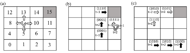
In this section, we provide numerical results for the rendezvous problem described in Sec. II. As in Fig. 2, the grid world is of size $4\times 4$, i.e. $n=4$, and it contains one goal point at the right-top position. Environment states are numbered row-wise starting from the left-bottom as shown in Fig. 2(a). All the algorithms are run for $50$ independent epochs. For each agent $i$ the initial state si,t=1eโˆ‰๐’ฎTesubscriptsuperscript๐‘ ๐‘’๐‘–๐‘ก1subscriptsuperscript๐’ฎ๐‘’๐‘‡s^{e}_{i,t=1}\notin\mathcal{S}^{e}_{T} in each episode is drawn uniformly from all non-terminal states.

We compare the conventional communication and the learned communication schemes reviewed in the previous section. Conventional communication transmits the position of an agent on the grid as the 4-bit binary version of the indices in Fig. 2(a) after encoding via a binary cyclic ($B$,4) code, where the received message is decoded by syndrome decoding.

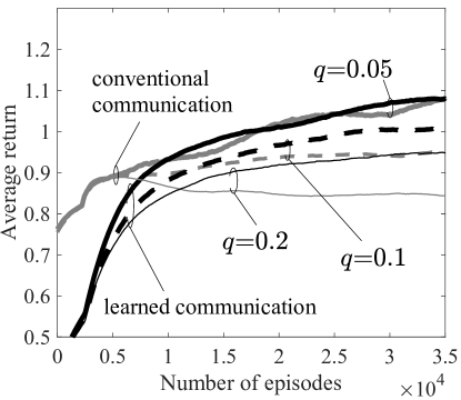
The performance of each scheme is evaluated in terms of the discounted return in (5), averaged over all epochs and smoothed using a moving average filter of memory equal to 4,000 episodes. The rewards in (3) are selected as $R_{1}=1$ and $R_{2}=3$, while the discount factor is $\gamma=0.9$. A constant learning rate $\alpha=0.15$ is applied, and the exploration rate $c$ of the UCB policy is selected from the set $\{0.3,0.4,0.5\}$ such that it maximizes the average return at the end of the episodes in an epoch.

We first investigate the impact of the channel noise by considering different values of the bit flip probability $q$. In Fig. 3 it is observed that conventional communication performs well at the low bit flipping rate of $q=0.05$, but at higher rates of $q$ learned communication outperforms conventional communication after a sufficiently large number of episodes. Importantly, for $q=0.2$, the performance of conventional communication degrades through episodes due to the accumulation of noise in the observations, while learned communication is seen to be robust against channel noise.

Refer to caption
Figure 3: Average return for conventional communication and learned communication when $B=7$.

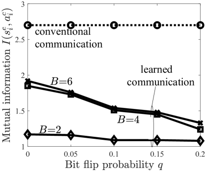
We now discuss the reasons that underlie the performance advantages of learned communication. We start by analyzing the capability of learned communication to compress the environment state information before transmission. To obtain quantitative insights, we measure the mutual information $I({\mathrm{s}^{e}_{i};\mathrm{a}^{c}_{i}})$ between the environment state $\mathrm{s}^{e}_{i}$ and the communication action $\mathrm{a}^{c}_{i}$ of an agent $i$ as obtained under the policy learned after 20,000 episodes for $q=0,0.05,0.1,0.15,0.2$. Fig. 4 plots the mutual information as a function of the bit flipping probability $q$ for learned communication. For conventional communication scheme the communication message $a^{c}_{i}$ is a deterministic function of the state siesubscriptsuperscript๐‘ ๐‘’๐‘–s^{e}_{i} and hence we have $I(\mathrm{s}^{e}_{i};\mathrm{a}^{e}_{i})=H(\mathrm{s^{e}_{i}})$, which is independent of $q$ and $B$. In the absence of channel noise, i.e., $q=0$, learned communication compresses by almost 30% the information about the environment state distribution $\mathrm{s}^{e}_{i}$ when $B=6$. This reduction becomes even more pronounced as the channel noise increases or when agents have a tighter bit-budget.

Refer to caption
Figure 4: Mutual information between an agentโ€™s environment state $\mathrm{s}^{e}_{i}$ and the communication action $\mathrm{a}^{c}_{i}$ versus the bit flip probability $q$ for conventional communication and learned communication with delay after 20,000 episodes ($B=2,4,6$,โ€‰ q=0.05,0.10,0.15,0.20๐‘ž0.050.100.150.20q=0.05,0.10,0.15,0.20).

We proceed by investigating how compression is carried out by jointly optimizing the agentโ€™s environment action and communication action policies. We will also see that learned communication carries out a form of unequal error protection. To this end, Fig. 5 illustrates a sample of the learned action and communication policies $\pi^{e}_{i}$ and $\pi^{c}_{i}$ for agent $i=1$ when $q=0.05$ and $B=4$ after 30,000 episodes of training in the presence of communication delays. In this figure, arrows show the dominant environment action(s) $a^{e}_{i}$ selected at each location; the bit sequences represent the communication action $a^{c}_{i}$ selected at each location; and the colour of each square shows how likely it is for the position to be visited by agent $i$.

Refer to caption
Figure 5: Illustration of a learned communication action policy when there is no communication delay ($B=4$, $q=0.05$). Locations with brighter colors are more likely to be visited. Arrows show the dominant action selected at any location. Bit strings show the message sent at a certain location.

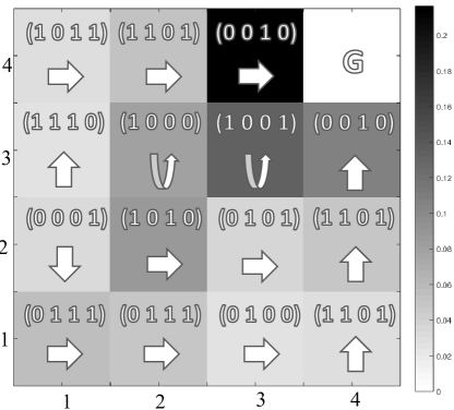
We can observe that compression is achieved by assigning same message to different locations. In this regard, it is interesting to note the interplay with the learned action policy: groups of states are clustered together if states have similar distance from the goal point, such as $\{\langle 4,3\rangle,\langle 3,4\rangle\}$ and $\{\langle 4,2\rangle,\langle 2,4\rangle\}$; or if they are very far from the goal point such as $\{\langle 1,2\rangle,\langle 1,3\rangle\}$. Furthermore, it is seen that the Hamming distance of the selected messages depends on how critical it is to distinguish between the corresponding states. This is because it is important for an agent to realize whether the other agent is close to the terminal point.

V Conclusions

In this paper we have studied the problem of decentralized control of agents that communicate over a noisy channel. The results demonstrate that jointly learning communication and action policies can significantly outperform methods based on standard channel coding schemes and on the separation between the communication and control policies. We observed this performance gain for delayed and noisy inter-agent communication and we discussed that the underlying reason for the improvement in performance is the learned ability of the agents to carry out data compression and unequal error protection as a function of the action policies.

VI Acknowledgements

The work of Arsham Mostaani, Symeon Chatzinotas and Bjorn Ottersten is supported by European Research Council (ERC) advanced grant 2022 (Grant agreement ID: 742648). Arsham Mostaani and Osvaldo Simeone have received funding from the European Research Council (ERC) under the European Unionโ€™s Horizon 2020 Research and Innovation Program (Grant Agreement No. 725731).

References

  • [1] D.ย V. Pynadath and M.ย Tambe, โ€œThe communicative multiagent team decision problem: Analyzing teamwork theories and models,โ€ Journal of Artificial Intelligence Research, vol. 16, pp. 389โ€“423, Jun. 2002.
  • [2] G.ย Weiss, Multiagent systems: a modern approach to distributed artificial intelligence, MIT press, 1999.
  • [3] M.ย Tan, โ€œMulti-agent reinforcement learning: Independent vs. cooperative agents,โ€ San Francisco, CA, USA, 1998, pp. 487โ€“494, Morgan Kaufmann Publishers Inc.
  • [4] L.ย Busoniu, R.ย Babuska, and B.ย D. Schutter, โ€œA comprehensive survey of multiagent reinforcement learning,โ€ IEEE Trans. Systems, Man, and Cybernetics, Part C, vol. 38, no. 2, pp. 156โ€“172, Mar. 2008.
  • [5] M.ย Lauer and M.ย A. Riedmiller, โ€œAn algorithm for distributed reinforcement learning in cooperative multi-agent systems,โ€ in Proc. Conference on Machine Learning. 2000, pp. 535โ€“542, Morgan Kaufmann Publishers Inc.
  • [6] A.ย Sahai and P.ย Grover, โ€œDemystifying the witsenhausen counterexample [ask the experts],โ€ IEEE Control Systems Magazine, vol. 30, no. 6, pp. 20โ€“24, Dec. 2010.
  • [7] F.ย Fischer, M.ย Rovatsos, and G.ย Weiss, โ€œHierarchical reinforcement learning in communication-mediated multiagent coordination,โ€ in Proc. IEEE Joint Conference on Autonomous Agents and Multiagent Systems, 2004. AAMAS 2004., New York, Jul. 2004, pp. 1334โ€“1335.
  • [8] S.ย Sukhbaatar, R.ย Fergus, etย al., โ€œLearning multiagent communication with backpropagation,โ€ in Proc. Advances in Neural Information Processing Systems, Barcelona, 2016, pp. 2244โ€“2252.
  • [9] J.ย Foerster, Y.ย Assael, N.ย D. Freitas, and Sh. Whiteson, โ€œLearning to communicate with deep multi-agent reinforcement learning,โ€ in Proc. Advances in Neural Information Processing Systems, Barcelona, 2016, pp. 2137โ€“2145.
  • [10] Q.ย Huang, E.ย Uchibe, and K.ย Doya, โ€œEmergence of communication among reinforcement learning agents under coordination environment,โ€ in Proc. IEEE Conference on Development and Learning and Epigenetic Robotics (ICDL-EpiRob), Sept. 2016, pp. 57โ€“58.
  • [11] J.ย Foerster, N.ย Nardelli, G.ย Farquhar, Ph. Torr, P.ย Kohli, and Sh. Whiteson, โ€œStabilising experience replay for deep multi-agent reinforcement learning,โ€ arXiv preprint arXiv:1702.08887, 2017.
  • [12] R.ย Lowe, L.ย Wu, A.ย Tamar, J.ย Harb, P.ย Abbeel, and I.ย Mordatch, โ€œMulti-agent actor-critic for mixed cooperative-competitive environments,โ€ in Proc. Advances in Neural Information Processing Systems, Long Beach, 2017, pp. 6382โ€“6393.
  • [13] J.ย N. Foerster, G.ย Farquhar, T.ย Afouras, N.ย Nardelli, and Sh. Whiteson, โ€œCounterfactual multi-agent policy gradients,โ€ arXiv preprint arXiv:1705.08926, 2017.
  • [14] Osvaldo Simeone, โ€œA very brief introduction to machine learning with applications to communication systems,โ€ IEEE Transactions on Cognitive Communications and Networking, vol. 4, no. 4, pp. 648โ€“664, 2018.
  • [15] R.ย Sutton and A.ย G. Barto, Introduction to reinforcement learning, vol. 135, MIT Press, 2 edition, Nov. 2017.