Investigating the Unusual Spectroscopic Time-Evolution in SN 2012fr

Abstract

The type Ia supernova (SN) 2012fr displayed an unusual combination of its Si II $\lambda\lambda$5972, 6355 features. This includes the ratio of their pseudo equivalent widths, placing it at the border of the Shallow Silicon (SS) and Core Normal (CN) spectral subtype in the Branch diagram, while the Si II$\lambda$6355 expansion velocities places it as a High-Velocity (HV) object in the Wang et al. spectral type that most interestingly evolves slowly, placing it in the Low Velocity Gradient (LVG) typing of Benetti et al. Only 5% of SNe Ia are HV and located in the SS+CN portion of the Branch diagram and less than 10% of SNe Ia are both HV and LVG. These features point towards SN 2012fr being quite unusual, similar in many ways to the peculiar SN 2000cx. We modeled the spectral evolution of SN 2012fr to see if we could gain some insight into its evolutionary behavior. We use the parameterized radiative transfer code SYNOW to probe the abundance stratification of SN 2012fr at pre-maximum, maximum, and post-maximum light epochs. We also use a grid of W7 models in the radiative transfer code PHOENIX to probe the effect of different density structures on the formation of the Si II $\lambda 6355$ absorption feature at post-maximum epochs. We find that the unusual features observed in SN 2012fr are likely due to a shell-like density enhancement in the outer ejecta. We comment on possible reasons for atypical Ca II absorption features, and suggest that they are related to the Si II features.

1 Introduction

Type Ia Supernovae (SNe Ia) are precise distance indicators, and are thus useful for measuring the expansion of the universe (Branch, 1998). Defining features of SNe Ia include (i) the relationship between their light curve width and luminosity (Phillips, 1993), (ii) their peak luminosity-color relationship (Tripp, 1998), (iii) their high degree of spectroscopic homogeneity (Blondin et al., 2012), and (iv) their peculiar progenitors (Hoeflich et al., 2000). Efforts to sub-classify SNe Ia to increase their usefulness as “standard candles” have been numerous (Branch et al., 2005; Wang et al., 2012). Most classification groups are developed based on spectroscopic features that are common and/or unique to SNe Ia. However, a number of odd SNe Ia have proven difficult to classify, and so their study is of particular importance in understanding the effort to solve the “second parameter problem”. SN 2012fr is one such object which Contreras et al. (2018) has recently shown is a 2000cx-like SN Ia (Candia et al., 2003; Li et al., 2001)

SN 2012fr exploded in NGC 1365, in the Fornax Cluster, and was discovered on October 27, 2012 (Childress et al., 2013; Zhang et al., 2014; Contreras et al., 2018). The rise time to peak UVOIR bolometric luminosity (maximum light) was estimated at $16.5\pm 0.6$ days, with the explosion time occurring on October 26 (Contreras et al., 2018). The light curve shape parameter was found to be $\Delta m_{15}(B)=0.84\pm 0.03$ (Contreras et al., 2018), $\Delta m_{15}(B)=0.80$ mag (Childress et al., 2013, preliminary value as reported by Contreras to Childress), and $\Delta m_{15}(B)=0.85\pm 0.05$ mag (Zhang et al., 2014). Thus, SN 2012fr is a slow decliner and should be bright. SN 2012fr displayed a maximum absolute B-band magnitude of $M_{B_{\text{max}}}=-19.3$ mag (no errors reported) and its light curve decline-rate was unusually shallow for an SN Ia with such a fast rise-time (Contreras et al., 2018). SN 2012fr suffered little or no host-galaxy reddening (Contreras et al., 2018), so we made no corrections for it in this work. We did correct for the redshift of the host-galaxy, which is $z=0.0054$.

SN 2012fr does not fit nicely into existing classification schemes due to an unusual combination of spectral features (Childress et al., 2013; Zhang et al., 2014; Contreras et al., 2018). These spectroscopic oddities affected the wavelength regions that are most critical to existing SNe Ia classification schemes. Thus, developing a better understanding of the physical reasons for these features in SN 2012fr is important in the larger context of SNe Ia classification. The study of spectroscopically unusual SNe Ia is instrumental to developing an improved understanding of the explosion mechanism (Baron, 2014). Previous spectral studies of SN 2012fr have focused on explaining spectral features by directly analyzing spectra (Childress et al., 2013; Zhang et al., 2014). We expand on this work by analyzing SN 2012fr using both conventional and non-conventional modeling techniques.

This work is organized as follows. § 2 discusses the spectroscopic peculiarities of SN 2012fr and summarizes previous attempts to explain them. § 3 presents SYNOW fits to a time-series of spectra and describes their qualitative behavior at pre-maximum (§3.1), maximum light (§3.2), and post-maximum (§3.3) phases. § 4 introduces our investigation of possible unusual density structures using the parameterized deflagration model W7 in PHOENIX; In § 5, we introduce the goodness-of-fit parameters $\lambda_{\text{diff}}$ and $R_{\lambda 6355}$ and explain their usefulness in our study. § 6 presents the results of our analysis in PHOENIX; § 7 discusses implications of our results.

2 Spectroscopic Peculiarities of SN 2012fr

The most prominent spectroscopic anomaly in SN 2012fr is the time-evolution of its Si II $\lambda 6355$ absorption line. The Si II $\lambda 6355$ line is the defining feature of SNe Ia. It emerges just after explosion and persists past maximum light for $\sim 20$ days in most cases. Because of its uniqueness to SNe Ia, Si II $\lambda 6355$ is integral to most sub-classification schemes. Benetti et al. (2005) used the velocity evolution of the minimum of the Si II $\lambda 6355$ line, along with the light curve decline rate, $\Delta m_{15}(B)$, to classify SNe Ia. The subclassifications in the Benetti et al. (2005) system are the FAINT group, the High Velocity Gradient (HVG) group, and the Low Velocity Gradient (LVG) group. FAINT and HVG SNe Ia have fast Si II evolution, while in LVGs the Si II features evolve more slowly. Branch et al. (2009) and Wang et al. (2009) also made use of the Si II $\lambda 6355$ feature in their classification schemes. Branch et al. (2009) classified SNe Ia into four groups based on the pseudo-equivalent widths (pEWs) of the Si II $\lambda 5972$ and $\lambda 6355$ lines. These are the Core Normal (CN), Cool (CL) Broad Line (BL), and Shallow Silicon (SS) groups. Wang et al. (2009) classified SNe Ia based on the velocity of the $\lambda 6355$ line, with those having Si II velocities at or above $11800$ $\text{km}~{}\text{s}^{-1}$ being classified as High Velocity (HV) events.

Typically, HV Si II $\lambda 6355$ absorption is accompanied by HVG time-evolution. As such, there is a high degree of overlap between the Wang et al. (2009) HV group and the Benetti et al. (2005) HVG group (Silverman et al., 2012). Conversely, low velocity (LV) absorption is usually accompanied by LVG features. However, SN 2012fr belongs to both the Benetti LVG and Wang HV groups. Furthermore, SN 2012fr lies on the border of the Branch CN and SS groups, which is an unusual classification in the Branch scheme for Wang HV events (Contreras et al., 2018; Stritzinger et al., 2018). Figure 1 displays a sampling of spectra ranging from day $-15$ to day $+22$ with respect to maximum light. All the spectra in this figure are those published in Childress et al. (2013), except the day $+12$ and day $+22$ spectra, which were published in Zhang et al. (2014). At day $-15$ (2 days after explosion), strong Si II $\lambda 6355$ absorption is centered near $5870$ Å ($\approx 23,000~{}\text{km}~{}\text{s}^{-1}$), which suggests a thick HV Si II layer. This is much faster (and earlier) than usual for Si II (for SN 2011fe, the Si II minimum formed at $6050\text{\AA}$). By day $-8$, the HV component is weak and the familiar, slower absorption feature centered near $6100$ Å appears and grows stronger, peaking in strength near maximum light. Childress et al. (2013) estimated a Si II velocity of $\approx 12000$ $\text{km}~{}\text{s}^{-1}$ at late times, but its temporal evolution is shallow, as shown by the vertical red line in Figure 1 that approximately bisects the minimum of the $\lambda 6355$ absorption trough from day $-8$ onward. Furthermore, Si II $\lambda 6355$ remains visibly distinct from Fe II absorption at day $+22$ past maximum light and even up to day $+39$ according to Childress et al. (2013); Contreras et al. (2018).

Absorption features of Ca II are also characteristic of SNe Ia. At epochs prior to maximum light, HV Ca II H&K tends to dominate, producing strong absorption features in the $3500-4000$ Å wavelength region. These features usually become weak by maximum light and are replaced at post-maximum phases by the Calcium Infrared Triplet (Ca IR3), which forms in the $8000-8500~{}\text{\AA}$ region (Branch et al., 2007). Typically, Ca II H&K forms in two distinct components: a high-velocity detached component, with the detached component fading by maximum light and a photospheric component. However, in SN 2012fr, High Velocity Features (HVFs) of Ca II H&K persist past maximum light. As seen in Figure 1, strong absorption between $3500$ and $4000$ Å is evident between day $-8$ and day $+8$ . Moreover, the Ca II $\lambda 8494$, $\lambda 8542$, and $\lambda 8602$ lines, which form the Ca IR3 feature, are remarkably unblended at late times (Childress et al. (2013), see their Figure 10). Several other SNe Ia with similar Ca II features also displayed the same kind of unusual Si II behavior observed in SN 2012fr. The objects include SN 2000cx, SN 2006is, SN 2009ig, and SN 2013bh (Contreras et al., 2018; Silverman et al., 2013). It is not surprising, then, that Childress et al. (2013) found that Ca II and Si II share a similar two-component structure and that their velocity evolution at early and late phases are analogous. Zhang et al. (2014) noticed similar features and emphasized the predominance of intermediate mass elements (IMEs) including Si II and Ca II at early times. Both concluded from these observations that Si II and Ca II are likely confined within a narrow range of velocities in SN 2012fr. Childress et al. (2013) argued that SN 2012fr has a narrowly confined shell-like distribution of IMEs persisting to late times. Zhang et al. (2014) similarly proposed that SN 2012fr is viewed at an angle from which the mass distribution is clumpy or shell-like in the outer ejecta. The goal of this paper is to test these assertions.

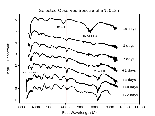
Figure 1: Rest frame sample of SN 2012fr spectra ranging from day $-15$ to day $+22$ with respect to maximum light. The vertical red line through $6100$ Å denotes the center of the Si II $\lambda 6355$ absorption feature from day $-8$ to day $+22$, which is the PVF component of the feature. The HVF components of Si II and Ca II IR3 are labeled in the day $-15$ plot. The HVF component of Ca II H&K can be seen at day $+8$ but not at day $+18$, and the PV Ca II IR3 feature becomes prominent at abound the time HV Ca II H&K starts to weaken. Data obtained from Childress et al. (2013) and Zhang et al. (2014).

3 SYNOW

We used the radiative transfer code SYNOW (Fisher, 2000) to fit a time-series of $10$ spectra ranging from day $-15$ to day $+18$ with respect to maximum light. SYNOW assumes homologous expansion $(v\propto r)$, spherical symmetry, a sharp photosphere with blackbody emission, and line formation by resonance scattering. SYNOW’s main advantage is that it takes multiple scattering into account (Branch et al., 2005). One disadvantage is that its free parameter space is large. SYNOW takes the photospheric velocity $v_{\text{phot}}$ and blackbody temperature $T_{\text{bb}}$ as global free parameters. For each ion, SYNOW takes the minimum and maximum velocities of each ion ($v_{\text{min}}$ & $v_{\text{max}}$), the e-folding velocity $v_{e}$ (explained below), the optical depth ($\tau$) of a reference line at $v_{\text{min}}$ for that ion, and the thermal excitation temperature $T_{\text{exec}}$. These parameters make SYNOW a useful tool for making line identifications and constraining ions to velocity intervals. However, SYNOW is not very helpful for making precise measurements because it does not give information on absolute abundances, rather only on the presence of a specific ion. Additionally, some parameters are degenerate. We use it here to explore possible reasons for the behavior of Si II and Ca II, particularly Si II, primarily on a qualitative level. We also use it to describe the relative evolution of other prominent ions in SN 2012fr.

The global fitting parameters and line optical depths used in our fits are given in Table 1. Although $T_{\text{exec}}$ can be set for each ion, we held it fixed at $10000$ K for all ions up to day $+1$ and $7000$K after that, to reduce the size of parameter space, as was done in Branch et al. (2007) and Branch et al. (2008). We constrained $T_{\text{bb}}$ to $16000$ or $15000$ K at all phases (except at day $-15$, for which $T_{\text{bb}}=7000$ K, and at day $+18$, for which $T_{\text{bb}}=9000$ K), although previous studies have shown that this parameter is not physically meaningful, because Type Ia’s are not even approximately true blackbodies and SYNOW only treats line scattering. (Bongard et al., 2008).

We employ a somewhat flexible definition of $v_{\text{phot}}$ in this study. In some cases, we found it helpful to define the $v_{\text{phot}}$ parameter lower than the minimum velocities (described below) of photospheric ions. In these cases, we give both $v_{\text{phot}}$ and $v_{\text{min}}$, but describe $v_{\text{min}}$ for the photospheric ions to be the “true” photospheric velocity. Clearly, in such cases all lines are detached. At day $+1$, $v_{\text{phot}}$ is consistent with previous fits to CN and SS Branch-type SNe Ia near-maximum light, with the notable exception of SN 2002cx (Branch et al., 2006). We note, however, that our $+8$ day $v_{\text{phot}}$ value of $12000$ $\text{km}~{}\text{s}^{-1}$ is $2000$ $\text{km}~{}\text{s}^{-1}$ less than the corresponding value found by Childress et al. (2013). A possible reason for this discrepancy will be explained in §3.2. We relegate many of the figures showing detailed SYNOW fits to Appendix A.

Table 1: Global SYNOW Fitting Parameters and Ion Optical Depths

Parameter	Day $-15$	Day $-12$	Day $-8$	Day $-5$	Day $-2$	Day $+1$	Day $+4$	Day $+8$	Day $+12$	Day $+18$
$v_{\text{phot}}\text{ ($10^{3}$ km $s^{-1}$)}\tablenotemark{*}$	$20/21$	$14$	$13.5$	$13$	$12.7/13$	$12.8$	$11.5/12.5$	$11/12$	$11/12$	$11$
$T_{\text{bb}}(\text{ K})$	$7000$	$16000$	$16000$	$16000$	$15000$	$16000$	$16000$	$16000$	$15000$	$9000$
$T_{\text{exec}}(\text{ K})$	$1000$	$10000$	$10000$	$10000$	$10000$	$10000$	$7000$	$7000$	$7000$	$7000$
$\tau(\text{{Na~{}I}})$	$\cdots$	$\cdots$	$\cdots$	$\cdots$	$0.1$	$0.3$	$0.3$	$0.5$	$0.3$	$0.4$
$\tau(\text{{Mg~{}II}})$	$\cdots$	$2.5$	$1.5$	$1.3$	$1.5$	$1.2$	$1.5$	$1.8$	$1.0$	$1.5$
$\tau(\text{{Si~{}II}})$	$\cdots$	$\cdots$	$3.5$	$3.5$	$6.0$	$8.0$	$7.0$	$6.0$	$5.5$	$4.0$
$\tau(\text{HV {Si~{}II}})$	$1.5$	$0.6$	$0.8$	$0.5$	$0.5$	$0.8$	$0.6$	$0.3$	$0.5$	$0.3$
$\tau(\text{{Si~{}III}})$	$2.5$	$1.5$	$2.5$	$2.5$	$1.0$	$\cdots$	$\cdots$	$\cdots$	$\cdots$	$\cdots$
$\tau(\text{{S~{}II}})$	$1.7$	$1.1$	$2.5$	$1.9$	$1.8$	$1.8$	$0.8$	$0.4$	$0.3$	$0$
$\tau(\text{{Ca~{}II}})$	$1.0$	$1.5$	$2.0$	$2.5$	$5.0$	$20$	$10$	$30$	$50$	$100$
$\tau(\text{HV {Ca~{}II} H\&K})$	$20$	$15$	$2.7$	$3.0$	$6.0$	$3.5$	$2.0$	$2.0$	$1.5$	$2.0$
$\tau(\text{{Fe~{}II}})$	$0.3$	$0.5$	$0.4$	$0.4$	$0.8$	$0.7$	$2.0$	$3.3$	$5.0$	$8.0$
$\tau(\text{{Fe~{}III}})$	$1.0$	$0.8$	$0.7$	$0.6$	$1.2$	$1.5$	$0.6$	$0.8$	$0.6$	$0.4$
$\tau(\text{{Co~{}II}})$	$\cdots$	$\cdots$	$\cdots$	$\cdots$	$0.2$	$1.0$	$0.3$	$0.5$	$1.0$	$2.0$

In SYNOW, the reference line optical depth of each ion as a function of velocity is approximated by

$$\centering\tau(v)=\tau(v_{\text{min}})e^{-(v-v_{\text{min}})/v_{e}},\@add@centering$$ (1)

where $\tau(v_{\text{min}})$ is the SYNOW input for that ion. Smaller values of $v_{e}$ produce a higher rate of decay of $\tau$ as v increases. The result is that $\tau$ and $v_{e}$ are partially degenerate (Branch et al., 2006). Some interesting trends are evident from the evolution of line optical depths. Ca II H&K is consistently fit with distinct HV and photospheric velocity (PV) components. The PV component is optically thin at early times and strengthens monotonically with time, becoming quite thick by day $+18$. The HV component (Ca II H&K) begins optically thick, declines rapidly, then increases again and reaches a local maximum at day $-2$. Si II displays the same type of two-component behavior as Ca II, although its HV component has a much lower $\tau$ than its PV component ($0.3\leq\tau(\text{HV {Si~{}II}})\leq 0.7$) in all later fits. The velocity parameters for each of the fits are given in Table 2. The top half of the table gives $v_{\text{min}}$ and $v_{\text{max}}$ for each ion and the bottom half gives $v_{e}$. Ions with minimum velocities greater than the PV are referred to as “detached.” The behavior of $v_{\text{min}}$, $v_{\text{max}}$, and $v_{e}$ are discussed for pre-maximum, maximum light, and post-maximum phases in § 3.1, § 3.2, and § 3.3, respectively.

Table 2: SYNOW Velocity Parameters in $10^{3}$ km $s^{-1}$

Parameter	Day $-15$	Day $-12$	Day $-8$	Day $-5$	Day $-2$	Day $+1$	Day $+4$	Day $+8$	Day $+12$	Day $+18$
$v_{\text{min}},v_{\text{max}}$ (Na I)	$\cdots$	$\cdots$	$\cdots$	$\cdots$	$16,19$	$14,16$	$12.5,16$	$12,15$	$12,16$	$11,15.5$
$v_{\text{min}},v_{\text{max}}$ (Mg II)	$\cdots$	$19,24$	$17.5,22$	$17,23.5$	$15.5,20.5$	$15.5,20$	$13.5,17.5$	$12.7,16.5$	$12,16$	$11,14$
$v_{\text{min}},v_{\text{max}}$ (Si II)	$\cdots$	$\cdots$	$13.5,16$	$14,16$	$14,15.5$	$14,16$	$14,15.5$	$14,15.5$	$13.8,15.5$	$13.5,15$
$v_{\text{min}},v_{\text{max}}$ (HV Si II)	$25,37$	$22,34$	$16,21$	$16,20$	$15.5,19$	$16,18.5$	$15.5,18$	$15.5,18$	$15.5,18$	$15,17$
$v_{\text{min}},v_{\text{max}}$ (Si III)	$23,28$	$17,21$	$14,16$	$13,15$	$13,15$	$\cdots$	$\cdots$	$\cdots$	$\cdots$	$\cdots$
$v_{\text{min}},v_{\text{max}}$ (S II)	$21,24$	$14,19$	$13.5,16$	$13,16.7$	$13,16$	$12.8,16$	$12.5,16$	$14,16$	$12,14$	$\cdots$
$v_{\text{min}},v_{\text{max}}$ (Ca II)	$21,26$	$14,25$	$13.5,18$	$13,19.2$	$13,17$	$12.8,16.8$	$12.5,16$	$12,15$	$12,15$	$11,15$
$v_{\text{min}},v_{\text{max}}$ (HV Ca II H&K)	$30,48$	$29,35$	$22.5,34$	$22.7,31.7$	$21,33$	$20.5,29$	$20,27$	$17.5,25$	$17,23$	$18,23$
$v_{\text{min}},v_{\text{max}}$ (Fe II)	$21,28$	$14,19$	$13.5,20$	$13,20.7$	$12.7,19$	$12.8,16.5$	$11.5,15$	$12,15$	$12,15$	$11,13$
$v_{\text{min}},v_{\text{max}}$ (Fe III)	$23,28$	$17.5,24.5$	$14,18$	$15,17.5$	$14,16$	$12.8,17.5$	$11.7,14.5$	$11.5,15$	$11.5,14.5$	$11,13.5$
$v_{\text{min}},v_{\text{max}}$ (Co II)	$\cdots$	$\cdots$	$\cdots$	$\cdots$	$13,15$	$12.8,13.5$	$12.5,14.5$	$12,14$	$11.5,13.5$	$11,13.5$
$v_{e}$ (Na I)	$\cdots$	$\cdots$	$\cdots$	$\cdots$	$1.0$	$1.0$	$1.0$	$1.0$	$8.0$	$10$
$v_{e}$ (Mg II)	$\cdots$	$1.0$	$1.0$	$1.0$	$1.0$	$1.0$	$1.0$	$1.0$	$1.0$	$1.0$
$v_{e}$ (Si II)	$\cdots$	$\cdots$	$1.0$	$1.0$	$1.0$	$1.0$	$1.0$	$1.0$	$1.0$	$1.0$
$v_{e}$ (HV Si II)	$4.0$	$5.0$	$1.0$	$1.0$	$1.0$	$1.0$	$1.0$	$1.0$	$1.0$	$1.0$
$v_{e}$ (Si III)	$1.0$	$1.0$	$1.0$	$1.0$	$1.0$	$\cdots$	$\cdots$	$\cdots$	$\cdots$	$\cdots$
$v_{e}$ (S II)	$1.0$	$1.0$	$1.0$	$1.0$	$1.0$	$1.0$	$1.0$	$1.0$	$1.0$	$\cdots$
$v_{e}$ (Ca II)	$4.0$	$4.0$	$3.0$	$3.0$	$4.0$	$3.0$	$3.0$	$4.0$	$3.0$	$4.0$
$v_{e}$ (HV Ca II H&K)	$10$	$10$	$10$	$7.0$	$4.0$	$5.0$	$6.0$	$5.0$	$4.0$	$4.0$
$v_{e}$ (Fe II)	$1.0$	$1.0$	$1.0$	$1.0$	$2.0$	$4.0$	$2.0$	$2.0$	$2.0$	$8.0$
$v_{e}$ (Fe III)	$2.0$	$1.0$	$1.0$	$1.0$	$1.0$	$1.0$	$1.0$	$1.0$	$1.0$	$1.0$
$v_{e}$ (Co II)	$\cdots$	$\cdots$	$\cdots$	$\cdots$	$1.0$	$5.0$	$1.0$	$1.0$	$3.0$	$5.0$

3.1 Pre-Maximum Light

From day $-15$ to day $-8$, the spectra of SN 2012fr were dominated by HVFs. At day $-15$ and day $-12$, HV Ca II H&K and Si II absorption was exceptionally strong. Figures 2 and A1 show the SYNOW fits at these times. At both phases, the Ca IR3 is unresolved, which is not reflected well in the fits despite large values of $v_{e}$ and $\tau(\text{HV {Ca~{}II}})$. At day $-15$, the speed of the IR3 and H&K absorption was correctly fit with a Ca II distribution stretching up to $48000$ $\text{km}~{}\text{s}^{-1}$ $\approx 0.16$c (in agreement with Childress et al., 2013), although it is unlikely that this speed is physical. Our fitted $\tau$ and $v_{e}$ are also large for the HV Si II feature. O I $\lambda 7773$ can account for some of the additional absorption in this region, but not all of it. PV Si II is not identified at these phases and the PV Ca II component is weak. Evidence for PV S II is found at both times, as reflected by the reasonable fits to the $5000-6000$ Å region, where the characteristic “Sulfur W” becomes distinct as the SN evolves to maximum brightness. Detached Mg II in the same velocity region as HV Si II and Ca II is also likely at day $-12$, although we find no evidence for Mg II at day $-15$. Si III $\lambda 4338.5$ may be present, although it is partially degenerate with Mg II $\lambda\lambda 4338.6$ because the two ions are used to fit the same features. Hence, we confirm the assertion by Childress et al. (2013) that the early-time spectra are dominated by IMEs.

Figure 2: Day $-12$ spectrum and two SYNOW fits. The fit in red does not contain any C II, while the dashed blue fit does. The Ca IR3 fit feature is not well-blended in the fit as it is in the observed spectrum. Also, adding C II decreases the quality of the fit near $6300$ Å as shown in the inset.

We tested for C II $\lambda 6580$ absorption by adding C II to the day $-12$ fit with a low optical depth of $\tau=0.02$ in a velocity range of $v_{\text{min}},v_{\text{max}}=17-19\times 10^{3}$ $\text{km}~{}\text{s}^{-1}$. The fits with and without C II are shown in Figure 2. We find that even optically thin C II produces a worse fit near $6300$ Å and so we did not include this feature in Tables 1 and 2. Therefore, if there is any C II present at early times in SN 2012fr, it is too weak to be confirmed by SYNOW in the Optical. However, a full search for C II would include a consideration of the NIR (see the analysis performed by Marion et al. (2015) of SN 2014J), which is beyond the scope of this work. This observation confirms the conclusions reached by Childress et al. (2013) and Zhang et al. (2014). Fe II and Fe III lines are present, although they are weak at early phases, as expected (Branch et al., 2006). We note that $v_{\text{phot}}$ evolves rapidly between day $-15$ and day $-12$, but quickly flattens out after this, as shown in Figure 3.

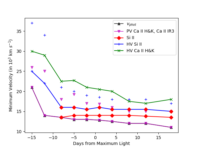
Figure 3: Minimum and maximum velocities of all components of Ca II and Si II, as well as $v_{\text{phot}}$ vs. time WRT maximum light. The minimum ion velocity is used here for $v_{\text{phot}}$ rather than the actual parameter value (see note on Table 2). Maximum velocity points are not connected by lines in the figure, to distinguish them from the corresponding minimum velocities. We also did not include the maximum velocity for HV Ca II H&K because it distorts the velocity scale and is not as important as the others. Note that the minimum HV and maximum PV Si II velocities are equal at day $-8$ and thereafter.

Fits to the day $-8$ and day $-5$ spectra are shown in Figure A1 (Appendix A). By day $-8$, the HV Si II feature has been largely replaced by a PV component. However, optically thin HV Si II remains distinct well after the PV component appears. We differentiate between the HV Si II denoted in Figures A1 and 2 and HV Si II absorption as defined in Tables 1 and 2. The former denotes visible absorption features blue-ward of $6000$ Å and the latter denotes fitted Si II with a minimum velocity greater than or equal to the maximum velocity of the PV component. HV Ca II H&K remains prominent surprisingly late, but PV Ca II  is necessary to produce the small but distinct absorption feature near $3900$ Å. The two components remain detached from each other up to day $+4$ and possibly afterward. Fe III is found to be detached from the photosphere, particularly at day $-5$. S II becomes more prominent at this stage, while Mg II weakens but stays detached.

The detachment of Ca II, Si II, Mg II, and even Fe III at pre-maximum phases implies that SN 2012fr is highly stratified before maximum light. The large width of HV Si II and Ca II absorption features at early times suggests the presence of processed IMEs at high velocities, since it is unlikely that the progenitor of SN 2012fr would contain that much primordial Si II and Ca II. By day $-5$, this layer has become optically thin, but remains identifiable in the fits. We note that while the HV component of Ca II remains detached from the PV component well past maximum light, there is no gap between the HV and PV components of Si II at day $-8$. Therefore, we find that the Ca II distribution in SN 2012fr is discontinuous, while the Si II distribution is continuous, but with a discontinuous $\tau$ gradient. S II displays roughly the same velocity evolution as PV Ca II, while Mg II behaves more like the HV Si II component, at least before maximum light. All of this suggests that the distribution of IMEs at pre-maximum phases have a complicated layered structure in which different ions dominate each layer.

3.2 Near Maximum Light

Near maximum light, PV components dominate the spectra of SN 2012fr, with the exception of Ca II H&K, which continues to have a prominent HV component. At day $-2$ (Figure 2) the HV and PV components of Si II have merged, occupying the range of $14000-19000$ $\text{km}~{}\text{s}^{-1}$, although at different optical depths. As mentioned, $\tau(PV\text{{Si~{}II}})$ peaks at maximum light and decreases steadily afterwards. The first evidence for optically thin Na I is found at day $-2$. However, the fit to the region where Na features typically form ($5700-6000$ Å) is not good at day $-2$ or $+1$, so Na I may not be present at this phase (or later). Ca IR3 absorption is relatively weak by this time, but the Ca H&K feature remains prominent, with distinct HV and PV Ca II being needed to obtain a good fit. Fe II becomes more prominent at this phase and PV Co II appears for the first time.

As early as day $-5$ (Figure 2), the PV Si II distribution becomes detached from the photosphere and the Si II $\lambda 6355$ absorption line begins to narrow after that. Si III disappears at day $+1$, leaving a single-component Si feature with an optical depth gradient that is discontinuous at around $15500-16000$ $\text{km}~{}\text{s}^{-1}$. All the other ions are photospheric by day $+1$ except Na I, HV Ca II H&K, and Mg II (Figure 4). At day $+4$ (Figure A2), the detachment of Si II becomes more pronounced as the photosphere continues to recede but the minimum velocity of PV Si II remains fixed at $14000$ $\text{km}~{}\text{s}^{-1}$ . The Si II $\lambda 6355$ line becomes progressively narrower, reflecting the decreasing size of the velocity interval in which optically thick Si II is found. PV Ca II becomes optically thick at this phase and Ca IR3 begins to strengthen. Absorption lines of Fe in the $4500-5000$ Å region, which become distinct starting at day $+4$, are best fit when Fe II and Fe III are placed below the minimum velocities of the photospheric ions. This just reduces the effective optical depth, since SYNOW only calculates the region between $v_{phot}$ and $v_{max}$.

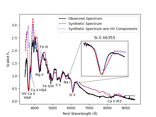
Figure 4: Day $+1$ spectrum and a synthetic SYNOW fit. The fit is plotted with and without the HV components of Si II and Ca II to illustrate their importance. The Si II $\lambda 6355$ line is enlarged in the inset to show the difference in the fits.

The defining feature of the temporal evolution near maximum light is the detachment of Si II, which becomes definite by day $-2$. Interestingly, the PV component of Ca II (as constrained by the PV H&K component ) does not behave this way, remaining truly photospheric at later times. This is the first major divergence between the behavior of PV Ca II and Si II, suggesting that Ca II reaches to much lower velocities than does Si II. This explains why the PV component of Ca II does not display the same LVG behavior at late times that Si II does.

3.3 Post-Maximum Light

At post-maximum phases, the Si II $\lambda 6355$ line becomes exceptionally narrow and PV Ca II becomes optically thick (as evidenced by the strengthening IR3 features). Lines of Fe II, including Fe II $\lambda 4924$, $\lambda 5018$, and $\lambda 5169$, also become more prominent at this stage. Figure A2 displays the fit to the day $+8$ spectrum. The defining feature here is the excellent fit to the Fe features in the range $4500-5000$ Å. These lines are exceptionally well-distinguished from each other, so they constrain the Fe II parameters quite well. Ca H&K is still fit reasonably well in the blue, but the IR3 feature is unresolved. Emission near $4000$ Å becomes much too strong starting at day $+8$, but this is likely an artifact of the blackbody approximation used in SYNOW. By day $+12$ (Figure A2), the absorption feature in the region of Si II $\lambda 5972$ broadens substantially, but by this phase the spectrum is dominated by Fe II absorption, so our identification of this feature with Si II $\lambda 5972$ is provisional. S II, still faintly visible in the small absorption feature near $5400$ Å at day $+8$, is essentially gone by day $+12$ and entirely absent in the day $+18$ fit (Figure A2).

The defining feature of the day $+12$ and day $+18$ spectra is the decreasing width of Si II $\lambda 6355$. The absorption feature of Si II $\lambda 6355$ remains distinct from strengthening Fe II lines as late as day $+39$, according to Childress et al. (2013). The minimum velocity does finally recede slightly, to $13500$ $\text{km}~{}\text{s}^{-1}$ by day $+18$, while the $\tau(\text{{Si~{}II}})$ discontinuity recedes to $15000$ $\text{km}~{}\text{s}^{-1}$ by that phase (Figure 3). However, it still evolves much more slowly in velocity space than the photosphere does, as illustrated in Figure 3. This type of Si II behavior at late times was identified by Branch (2001) in SN 1991bg. The PV component of Ca II in the fits does not become detached from the photosphere, but the HV component does remain identifiable and detached from the PV component. Therefore, the behaviors of Si II and Ca II continue to diverge at late times, suggesting that these ions are distributed differently at low velocities.

The confinement of Si II to a narrow interval of velocities and the late-time distinctiveness of the Si II $\lambda 6355$ line support the hypothesis that SN 2012fr may have a density enhancement after maximum light. But if there is a shell, it is unclear where it is located. At least three explanations are possible. First, there may be a high-velocity shell in the middle of the Si II distribution. In this case, we would expect Ca II and Si II to both be detached, unless Ca II is not abundant in the shell region. It is also possible that the narrow Si II absorption is produced by a steep density profile at high velocities. In this case, a shell at lower speeds might explain the shallow photospheric velocity noted by Contreras et al. (2018). Another possibility is that the abundance structure of SN 2012fr is sufficiently stratified to produce a structure involving multiple shells. The rest of this work is devoted to exploring the first two possibilities. Furthermore, in § 4 - 6, we investigate whether the strange behavior of SN 2012fr can be explained by only an abnormal density structure.

4 Density Modeling in PHOENIX

The shell-like behavior of Si II and Ca II at late times and the narrow width of the Si II $\lambda 6355$ line are independently suggestive of the presence of a shell and/or a steep density dropoff described above. Zhang et al. (2014) found that a value of $v_{e}$ lower than $1000$ $\text{km}~{}\text{s}^{-1}$ for Si II was needed to fit the maximum light Si II $\lambda 6355$ feature of SN 2012fr using SYNOW. We obtained nearly equivalent fits with $v_{e}=1000$ $\text{km}~{}\text{s}^{-1}$, but with an awkwardly discontinuous opacity gradient structure. It may be that there is actually one continuous opacity gradient with $v_{e}<1000$ $\text{km}~{}\text{s}^{-1}$. Either way, a possible interpretation of this result is that the density profile of SN 2012fr is steeper than most SNe, which are usually well-fitted with a single Si II component with $v_{e}\geq 1000$ $\text{km}~{}\text{s}^{-1}$ (Branch et al., 2006, 2007, 2008). This is an odd conclusion to reach, considering our earlier deduction that the region containing Si II may be shell-like. To try to explain this phenomenon, we examined the density structure of SN 2012fr more closely.

To probe the density structure of SN 2012fr, we used the parameterized deflagration model W7 (Nomoto et al., 1984) converged with the radiation transfer code PHOENIX (Baron et al., 2006). We used W7 because it has a relatively simple abundance/density structure that was easy to manipulate and it fits the observed spectrum of SNe Ia relatively well near maximum light. Our focus was the formation of the Si II $\lambda 6355$ line at post-maximum phases. Note that the distribution of Si II in W7 is in good agreement with the velocity limits inferred from SYNOW at maximum light for SN 2012fr after being shifted $4000$ $\text{km}~{}\text{s}^{-1}$ to the right, as shown in Figure A4. Since there is no sharp photosphere in PHOENIX, an offset in velocity space is not surprising. The advantage of using PHOENIX here is that it can be used to probe the detailed physical structure of the model, not just to produce synthetic spectra. This allowed for direct manipulation of the density profile of W7. Models were converged in Local Thermal Equilibrium (LTE) for computational expediency. We simulated the qualitative features discussed above using three parameterized density modification procedures. Since W7 assumes homologous expansion, all physical manipulations were performed in velocity space. In each procedure, a W7 model was calculated to provide an unmodified reference density profile $\rho_{\text{ref}}(v)$. This profile was piecewise fit to a set of exponential and linear functions to obtain an “idealized” density profile $\rho_{\text{fit}}(v)$.

Next, $\rho_{\text{fit}}(v)$ was modified using three functions formulated to simulate the desired features. These are described in § 4.1, § 4.2, and § 4.3. Each was applied to the fit density on a range of velocities ($v_{\text{min}}$ to $v_{\text{max}}$) such that the new fit $\rho_{\text{new}}(v)$ is given by

$$\large\rho_{\text{new}}(v)=\begin{cases}\rho_{\text{mod}}(v)&v_{\text{min}}\leq v\leq v_{\text{max}},\\ \rho_{\text{fit}}(v)&\text{otherwise},\end{cases}$$ (2)

where $\rho_{\text{mod}}(v)$ is the modified density function added by the procedure. Finally, the reference profile was multiplied at every point by the ratio of the modified and unmodified fit densities, giving

$$\rho(v)=\rho_{\text{ref}}(v)\cdot\frac{\rho_{\text{new}}(v)}{\rho_{\text{fit}}(v)}.$$ (3)

The final step was to normalize the new density to conserve the mass of the reference profile. We integrate (using a trapezoidal approximation) to get the mass ratio $R_{m}$ as

$$R_{m}=\frac{\int_{v_{lower}}^{v_{upper}}\rho_{\text{ref}}(v)v^{2}\text{dv}}{\int_{v_{\text{lower}}}^{v_{upper}}\rho(v)v^{2}\text{dv}},$$ (4)

where $v_{\text{upper}}$ and $v_{\text{lower}}$ are the lower and upper velocity limits of the model. Models were then converged with density profile $R_{m}\rho(v)$. The advantage of this procedure is that local features of the W7 density that are not included in the idealized fit are preserved in the modified profile. This allows for an honest evaluation of the effects of the added features. We note that this method affects only the density structure of W7, it does not effect the velocity ranges where different ions are present, so the abundance structure is manipulated only indirectly. Future work will investigate whether a direct manipulation of the abundance stratification of W7 or some other model can best explain SN 2012fr.

4.1 Density Model: D0

Our first procedure, denoted D0, steepens the decay rate of $\rho(v)$ in the velocity region $v_{\text{min}}\leq v\leq v_{\text{max}}$, where $v_{\text{min}}$ and $v_{\text{max}}$ are parameters. The steepened profile is an exponential function with decay rate specified by $v_{e}$ (also a free parameter), as in SYNOW. The modified density function is

$$\rho_{\text{mod}}(v)=Ae^{-v/v_{e}}+B,$$ (5)

where $A$ and $B$ both have units of density and are chosen so that $\rho_{\text{mod}}(v_{\text{min}})=\rho_{\text{fit}}(v_{\text{min}})$ and $\rho_{\text{mod}}(v_{\text{max}})=\rho_{\text{fit}}(v_{\text{max}})$. This restriction ensures that $\rho_{\text{new}}(v)$ is continuous, but requires the shift parameter $B$. A D0 profile with parameters $v_{\text{min}}=10000$ $\text{km}~{}\text{s}^{-1}$, $v_{\text{max}}=17000$ $\text{km}~{}\text{s}^{-1}$ and $v_{e}=1000$ $\text{km}~{}\text{s}^{-1}$ is displayed in Figure 5 (left) with the corresponding day $+1$ fit to SN 2012fr (right). We observe that the endpoints of the modified profile are not precisely at $10000$ $\text{km}~{}\text{s}^{-1}$ and $17000$ $\text{km}~{}\text{s}^{-1}$. This is because the density grid in velocity space only contains $256$ bins, so a binning error of $\approx 100$ $\text{km}~{}\text{s}^{-1}$ is introduced. The local features of the W7 profile are “warped” to match the change to the global features.

Figure 5: W7 density profile with modified D0 profile (a) and corresponding day $+1$ fit (b) with the W7 fit with the unmodified profile included for comparison. The input parameters for this fit are $v_{min}=10,000$ $\text{km}~{}\text{s}^{-1}$, $v_{max}=17,000$ $\text{km}~{}\text{s}^{-1}$, and $v_{e}=1,000$ $\text{km}~{}\text{s}^{-1}$. Note that local features of the profile, such as the irregularity centered near $14,000$ $\text{km}~{}\text{s}^{-1}$, are preserved in D0. The flux spectra are normalized at $6260$ Å to make the $\lambda 6355$ line easy to compare, which is why the fit to the blue of $5800$ Å is vertically offset.

We held $v_{e}$ at $1000$ $\text{km}~{}\text{s}^{-1}$ to reduce the size of parameter space, and varied $v_{\text{min}}$ and $v_{\text{max}}$ over a reasonable range. This grid-based approach allowed us to explore the dependence of the Si II $\lambda 6355$ line on the D0 parameters. While D0 was able to reproduce the shape of the Si II absorption profile reasonably well, it placed the minimum of the line too far to the red. This implies that in D0, the line forming region of Si II is too far inside the ejecta and thus, at velocities that are too low.

4.2 Density Model: D1

Our second procedure, denoted D1, adds a shell-like density enhancement centered at a variable velocity $v_{c}$ with width and thickness parameters w and p. The shell is modeled by a “tilted Gaussian” function of the form

$$\rho_{\text{mod}}(v)=(p+1)*\rho_{\text{fit}}(v_{c})e^{-(v-v_{c})^{2}/a}+bv+c,$$ (6)

where $a$, $b$, and $c$ are free parameters chosen so that $\rho_{mod}(v)$ fits the points $(v_{c},(p+1)*\rho_{\text{fit}}(v_{c}))$, $(v_{c}-0.5w,\rho_{\text{fit}}(v_{c}-0.5w))$, and $(v_{c}+0.5w,\rho_{\text{fit}}(v_{c}+0.5w))$. The result is a shell centered near $v_{c}$ with approximate width $w$ and peak density close to $(p+1)*\rho_{\text{fit}}(v_{c})$. D1 reproduces the shell-like structure hypothesized in SN 2012fr with variable dimensions and position in velocity space. An example D1 profile with parameters $v_{c}=11000$ $\text{km}~{}\text{s}^{-1}$, $w=3000$ $\text{km}~{}\text{s}^{-1}$, and $p=2$, which clearly shows the effect of D1 on W7 and provides a reasonable fit, and the corresponding day $+1$ fit are shown in Figure 6. The fit to the Si II $\lambda 6355$ line is better than in D0 in terms of position, but the overall shape of the absorption profile is not quite the same as the observed feature. Also, the prominent absorption feature near $5750$ Å (a blend Si II $\lambda 5972$, Na I, and Fe II absorption) that is nearly absent in SN 2012fr is much stronger in D1 than in D0, at least for these parameters. D0 and D1 produce partially inverse effects when applied to the same velocity regions. D0 subtracts mass between $v_{\text{min}}$ and $v_{\text{max}}$, while D1 adds mass between $v_{c}-0.5w$ and $v_{c}+0.5w$. The fits in Figures 5 and 6 suggest that D0 does a better job of reproducing the shape of the SN 2012fr Si II absorption profile, but D1 correctly places the line in velocity space. Thus, they account for different aspects of the observed profile.

Figure 6: W7 Density Profile with modified D1 profile (a) and corresponding day $+1$ fit (b) with the W7 fit with the unmodified profile included for comparison. The input parameters for this fit are $v_{c}=11,000$ $\text{km}~{}\text{s}^{-1}$, $p=2$, and $w=3,000$ $\text{km}~{}\text{s}^{-1}$.

4.3 Density Model: D2

To determine how these features interact with each other, we parameterized a third procedure (denoted D2) that combines the effects of D0 and D1 by producing a shell at lower velocities and a steep density profile at higher velocities. D2 fits Equation 6 with a set of D1 parameters $v_{c}$, $w$, and $p$, then fits Equation 5 to $v_{\text{min}}=v_{c}+0.5w$ and $v_{\text{max}}=v_{u}$, where $v_{u}$ is a free parameter specifying the upper velocity limit for Equation 5. We fixed $v_{e}=1000$ $\text{km}~{}\text{s}^{-1}$ to reduce the size of parameter space. A D2 profile with parameters $v_{c}=11000$ $\text{km}~{}\text{s}^{-1}$, $w=3000$ $\text{km}~{}\text{s}^{-1}$, $p=2$ and $v_{u}=17000$ $\text{km}~{}\text{s}^{-1}$ is shown in Figure 7 (left) and corresponding day $+1$ fit (right). The fit to the Si II $\lambda 6355$ line is similar to Figure 6. This is not surprising, since the D1 component of the modification overlaps the W7 Si II distribution more than does the D0 component for these parameters. When $v_{c}$ is reduced with $v_{u}$ held fixed, the effect of D0 becomes more pronounced as more mass is removed from the Si II distribution.

W7 contains Si between $9000$ $\text{km}~{}\text{s}^{-1}$ and $16000$ $\text{km}~{}\text{s}^{-1}$ (Bongard et al., 2008), so we focused our analysis on that velocity region. In D1 and D2, we held p to either $1$, $2$ or $3$ and w to either $2000$ $\text{km}~{}\text{s}^{-1}$ or $3000$ $\text{km}~{}\text{s}^{-1}$. We varied the other parameters to sufficiently cover the $9000-16000$ $\text{km}~{}\text{s}^{-1}$ range. This process was repeated at selected phases to produce a time-series of grids. Because of the relatively small number of free parameters, we were able to accomplish a comprehensive analysis by converging on the order of $1000$ models. To quantitatively analyze the effect of these parameters on the Si II $\lambda 6355$ line, we developed goodness-of-fit parameters described in the next section.

Figure 7: W7 density profile with D2 profile (a) and corresponding day $+1$ fit (b) with the W7 fit with the unmodified profile included for comparison. The input parameters for this fit are $v_{c}=11,000$ $\text{km}~{}\text{s}^{-1}$, $p=2$, $w=3,000$ $\text{km}~{}\text{s}^{-1}$, and $v_{u}=17,000$ $\text{km}~{}\text{s}^{-1}$. Note that D2 adds mass at lower velocities and removes mass at higher velocities, so the effect of normalization on the rest of the profile is less than in either D0 or D1.

5 $\lambda_{\text{diff}}$ and $R_{\lambda 6355}$

To capture the behavior of the Si II$\lambda 6355$ line quantitatively, we developed a two-parameter metric for evaluating its goodness-of-fit to observed spectra. We defined parameters to (1) measure the relative minima of the synthetic and observed line and (2) capture their relative absorption strengths. First, we define

$$\large\lambda_{\text{diff}}=\lambda^{\text{obs}}_{\text{min}}-\lambda^{\text{syn}}_{\text{min}},$$ (7)

where $\lambda^{\text{obs}}_{\text{min}}$ is the wavelength that minimizes the observed flux, $F^{\text{obs}}_{\lambda}$ between $5970$ Å and $6220$ Å and $\lambda^{\text{syn}}_{\text{min}}$ is defined equivalently. Because the minimum of the Si II $\lambda 6355$ line depends on the average speed of the Si II distribution, $\lambda_{\text{diff}}$ is a measure of the difference of the average speeds of Si II in the synthetic and observed spectra. Positive values of $\lambda_{\text{diff}}$ indicate faster synthetic absorption. Note that $\lambda_{\text{diff}}$ is independent how the spectra are normalized.

To measure the relative absorption strength of the lines, we first define the continuum flux as the straight line that goes through the two points at $(F^{X}_{\lambda}(5970),F^{X}_{\lambda}(6220))$, where the superscript $X$ refers to synthetic or observed flux. Thus,

$$F^{X}_{\text{cont}}(\lambda)\equiv\left(\frac{F^{X}_{\lambda}(6220~{}\text{\AA})-F^{X}_{\lambda}(5970~{}\text{\AA})}{250\text{\AA}}\right)(\lambda-5970~{}\text{\AA})+F^{X}_{\lambda}(5970~{}\text{\AA}).$$ (8)

Then we define the ratio

$$R_{\lambda 6355}=\frac{\int_{5970~{}\text{\AA}}^{6220~{}\text{\AA}}\left(F^{\text{syn}}_{\text{cont}}(\lambda)-F^{\text{syn}}_{\lambda}(\lambda)\right)\,d\lambda}{\int_{5970~{}\text{\AA}}^{6220~{}\text{\AA}}\left(F^{\text{obs}}_{\text{cont}}(\lambda)-F^{\text{obs}}_{\lambda}(\lambda)\right)d\lambda},$$ (9)

where the subscripts syn and obs refer to the synthetic and observed flux, as in Equation 7. $R_{\lambda 6355}$ is conceptually similar to the ratio of the pseudo-equivalent line widths (pEWs) of Si II $\lambda 6355$ in the synthetic and observed spectra, with two important differences. First, the flux integrals are not normalized with respect to the continuum flux, so that differences in absorption strength can be compared. Note that this means that $R_{\lambda 6355}$ is sensitive to flux normalization, unlike the pEW. We account for this by normalizing all the spectra in the same place ($6260$ Å). Second, the wavelength interval used to calculate $R_{\lambda 6355}$ is held fixed at $5970-6220$ Å, rather than being selected for each individual spectrum based on the particular shape of the P-Cygni line (Nordin et al., 2011). Furthermore, the pEW is usually not considered when the pseudo-continuum becomes no longer accurately measurable due to Fe lines (Childress et al., 2013). However, $R_{\lambda 6355}$ retains its usefulness as a figure of merit because it measures how “washed out” the Si II line is by Fe features at these times. Moreover, $R_{\lambda 6355}$ accounts for differences in line width because the wavelength limits of the integral are independent of differences in pEW.

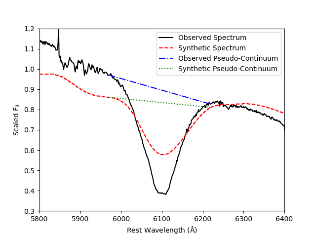
Figure 8: A W7 fit to the Si II $\lambda 6355$ line at day $+1$. The dashed blue line denotes the OPC, and the dashed green line the SPC. At day $+1$, $\lambda_{\text{diff}}=+5.55$ Å and $R_{\lambda 6355}=0.564$.

Figure 8 displays W7 fits to the Si II $\lambda 6355$ line at day $+1$ and day $+18$. In each plot, the solid blue line is the observed pseudo-continuum (OPC) from $5970-6220$ Å and the dashed blue line is the synthetic pseudo-continuum (SPC). In the day $+1$ fit (Figure 8), the OPC clearly approximates the continuum of the observed spectrum. The SPC is much flatter, but it still clearly denotes the area carved out by the synthetic Si II absorption.

We found that $\lambda_{\text{diff}}$ was slightly larger than $0$ in the unmodified fits and increased past maximum light. This systematic offset may be due to the fact that Si II $\lambda 6355$ is slightly too fast in W7 (Baron et al., 2006). Also, the presence of Fe features in that region at late times can have the effect of masking the true position of the Si II $\lambda 6355$ line. The doublet nature of the Si II $\lambda 6355$ line can also result in the flux minimum being offset from the true center by roughly $\pm 5-10$ Å. We also found that the synthetic Si II $\lambda 6355$ absorption profile in W7 was consistently too shallow. A perfect fit would produce $R_{\lambda 6355}=1$, but we found that $0.2\leq R_{\lambda 6355}\leq 0.65$ in nearly all our fits. Still, higher values of $R_{\lambda 6355}$ consistently correspond to better fits at fixed phases. We therefore focused on using $\lambda_{\text{diff}}$ and $R_{\lambda 6355}$ to make differential comparisons of the effects of changing inputs in D0, D1, and D2.

6 PHOENIX Results

We converged grids of W7 models at day $+1$, $+4$, $+8$, $+12$, and $+18$ in D0, D1, and D2. Luminosities were chosen for each phase based on the observed luminosity evolution of SN 2012fr. The goodness-of-fit of the Si II $\lambda 6355$ line was measured using $\lambda_{\text{diff}}$ and $R_{\lambda 6355}$. To compare the fixed-time effects of each procedure, we used the day $+1$ fits, which were generally the best. While all the input parameters affect the fits, the most significant for us are those which control the location of the modification in velocity space. In D0, we focused on the effect of changes in $v_{\text{max}}$ and in D1 and D2 we focused on $v_{c}$. We did this because $v_{\text{max}}$ determines the extent and prominence of the steepened region of the density profile in D0 and $v_{c}$ determines the location of the shell in D1 and D2. Thus, these parameters are most directly related to where mass is being added or subtracted in velocity space. Selected plots of $\lambda_{\text{diff}}$ and $R_{\lambda 6355}$ against velocity parameters of D0, D1, and D2 are shown in Figures 9 and  10.

Figure 9: $\lambda_{\text{diff}}$ (a) and $R_{\lambda 6355}$ (b) vs. $v_{\text{max}}$ (for D0 fits) at day $+1$ with $v_{\text{min}}$ and $v_{e}$ held fixed at $9000$ $\text{km}~{}\text{s}^{-1}$ and $1000$ $\text{km}~{}\text{s}^{-1}$, respectively. $\lambda_{\text{diff}}$ trends monotonically downward, while $R_{\lambda 6355}$ peaks at $v_{\text{max}}=15500$ $\text{km}~{}\text{s}^{-1}$. The values of $\lambda_{\text{diff}}$ and $R_{\lambda 6355}$ for unmodified W7 are included for comparison. (c): Fits to the Si II $\lambda 6355$ line for several values of $v_{\text{max}}$. Note that the lineshape is best fit with $v_{\text{max}}$ between $14000$ $\text{km}~{}\text{s}^{-1}$ and $16000$ $\text{km}~{}\text{s}^{-1}$, but the line is pushed too far to the red as $v_{\text{max}}$ increases.

As shown in Figure 9, increasing $v_{\text{max}}$ with $v_{\text{min}}$ and $v_{e}$ held fixed caused $\lambda_{\text{diff}}$ to decrease. This is not surprising. A steeper density profile would shift the mean of the Si II distribution to a lower velocity. More interesting is the sharp peak in $R_{\lambda 6355}$ at $15500$ $\text{km}~{}\text{s}^{-1}$, which indicates a maximum in absorption strength. The peak may be the result of weakening Si II $\lambda 5792$ absorption raising the flux at $5970$ Å, thus increasing the area under the SPC. The sharp decline in flux for values above $15500$ $\text{km}~{}\text{s}^{-1}$ is probably due to decreasing Si II opacity as more mass is removed from the $9000-16000$ $\text{km}~{}\text{s}^{-1}$ region and the corresponding red-ward movement of the absorption line. What this suggests is that the shape of the Si II $\lambda 6355$ line is slightly better fit by a density profile that falls off more quickly in the range where Si II is found than it does in unmodified W7.

Figure 10: $\lambda_{\text{diff}}$ (a) and $R_{\lambda 6355}$ (b) vs. $v_{c}$ (for D1 and D2 fits) at day $+1$ with w and p held fixed at $3000$ $\text{km}~{}\text{s}^{-1}$ and $2$, respectively. In the D2 models, $v_{u}$ is held fixed at $17000$ $\text{km}~{}\text{s}^{-1}$. In D1, $\lambda_{\text{diff}}$ increases monotonically and $R_{\lambda 6355}$ peaks at $9500$ $\text{km}~{}\text{s}^{-1}$. In D2, $\lambda_{\text{diff}}$ increases monotonically and $R_{\lambda 6355}$ peaks at $10500$ $\text{km}~{}\text{s}^{-1}$. The values of $\lambda_{\text{diff}}$ and $R_{\lambda 6355}$ for unmodified W7 are included for comparison. (c): D1 fits to the Si II $\lambda 6355$ line for several values of $v_{c}$. (d): D2 fits to the Si II $\lambda 6355$ line for several values of $v_{c}$.

As shown in Figure 10, increasing $v_{c}$ in D1 produces faster Si II absorption, as expected. Shifting a shell to higher speeds increases the average velocity of Si II. However, $R_{\lambda 6355}$ begins to fall off starting at $v_{c}=11000$ $\text{km}~{}\text{s}^{-1}$. This may be due to the broadening of the line as optically thick Si II is spread over a wider range of velocities. It may also be due to the strengthening of the Si II $\lambda 5972$ line, or an increase in the mass fraction of the HV Fe II mentioned earlier. To probe the significance of the HV Fe, we converted the ${}^{52}\text{Fe}$, ${}^{54}\text{Fe}$ and ${}^{56}\text{Fe}$ abundances in W7 to Si and re-converged the model. We found that the removal of HV Fe had a negligible effect on the formation of the $5500-6500$ Å region of the spectrum, suggesting that the strong absorption may be produced by the LV Fe that forms the continuum. Previous studies (such as Bongard et al., 2008) have shown that Fe absorption at low velocities significantly affects the shape of the continuum in certain wavelength regions at late time, including the region considered here.

In any case, we find that shells centered at high velocities ($\geq 11000$ $\text{km}~{}\text{s}^{-1}$) did not produce good fits. Better fits are obtained with the shell centered at $\leq 11000$ $\text{km}~{}\text{s}^{-1}$ and these produce stronger absorption profiles than the best fits using D0. Therefore, our preliminary analysis suggests that a shell centered somewhere below $11000$ $\text{km}~{}\text{s}^{-1}$ can account for SN 2012fr better than an unusually steep density profile.

Increasing $v_{c}$ in D2 (Figure 10) produces a more interesting effect. $\lambda_{\text{diff}}$ increases linearly, while $R_{\lambda 6355}$ peaks near $v_{c}=10500$ $\text{km}~{}\text{s}^{-1}$ at a value of $0.628$. Moreover, $\lambda_{\text{diff}}=-8$ Å at that point, so the position is reasonably well-fit (and improves in later fits). Figure 11 shows the day $+1$ D2 fit with unmodified W7 in blue for comparison. D2 parameters used are $v_{c}=10500$ $\text{km}~{}\text{s}^{-1}$, w = $3000$ $\text{km}~{}\text{s}^{-1}$, p = $2$, and $v_{u}=17000$ $\text{km}~{}\text{s}^{-1}$. Although the D1 fit at day $+1$ is actually slightly worse than W7, the overall D2 time series for these parameters does a better job of matching observations than W7. Figure 12 shows the fits at day $+4$ (left) and day $+8$ (right) using the same parameters. In both fits, the synthetic line is centered correctly and the absorption profile is a slightly better match than in the unmodified spectrum. Even at later times, when W7 ceases to resemble the observed spectra of SNe Ia in the $5500-6500$ Å wavelength region (Baron et al., 2006), the situation is still improved qualitatively. In Figure 13, the fit at day $+18$ (right) is shown for the same D2 parameters. At day $+18$, the Si II line is completely washed out by Fe features in the unmodified fit, but in the D2 fit faint Si II absorption remains distinct and correctly positioned.

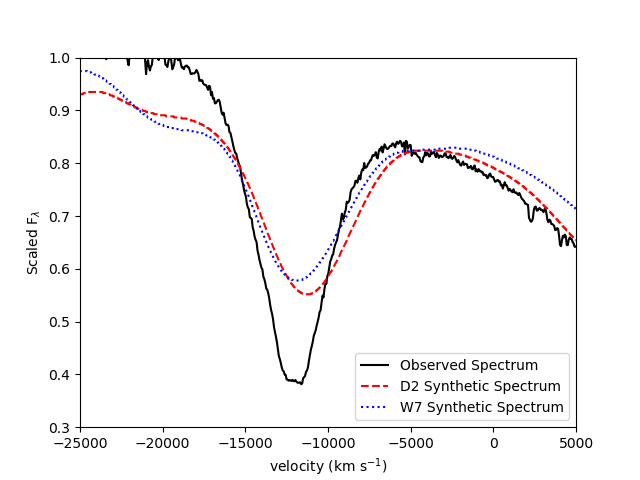
Figure 11: D2 fit (red) to the Si II $\lambda 6355$ line in SN 2012fr at day $+1$, with unmodified W7 fit (blue) for comparison, plotted in velocity space (negative velocities are indicate blue-shift). The profiles have nearly the same shape, the W7 profile being slightly too blue and the D2 profile being somewhat too red. Neither profile successfully captures the flat bottom (doublet feature) of the observed line. At this epoch, the D2 absorption trough is slightly deeper, but the wavelength minimum of W7 is closer to observations.

Figure 12: D2 fit at day $+4$ (left) and day $+8$ (right) with unmodified W7 for comparison.

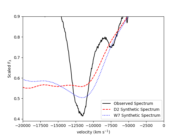
Figure 13: D2 fit at day $+18$ (right) with unmodified W7 for comparison.

It may be that constraining the Si II abundance in W7 to occupy a smaller range of velocities would produce a better result. We reemphasize that the procedures used here do not affect the velocities at which Si II is found or the mass fractions in each velocity bin, since they are density enhancements rather than abundance enhancements. By only modifying the density, we consider the effect of redistributing mass without changing the velocity intervals in which each ion is present. As mentioned earlier, Figure A4 indeed shows that the velocity extent of silicon in W7 well matches the velocity extent that we have inferred from our SYNOW fits. Due to the different treatments of radiative transfer, there is a global velocity offset between SYNOW and PHOENIX, but the velocity width is nearly the same. We modified only the density here because modifying the abundance distribution as well would produce a much larger parameter space. We do, of course, alter the optical depths at every point, both the Sobolev optical depths, which are not used in PHOENIX, and in general. Since PHOENIX does not use Sobolev optical depths the line formation in PHOENIX is much more complex than in SYNOW (Bongard et al., 2008). We note that since we ran over $1000$ models in this study, we ran them in Local Thermal Equilibrium (LTE) for computational expediency. However, NLTE effects are known to play an important role in the formation of the features being studied here (Baron et al., 2006)

7 Discussion

From the results presented in § 3, it is evident that the abundances in SN 2012fr are highly stratified at early and late times. HV components of Si II and Ca II occupy roughly the same velocity region at early times, possibly mixed with Mg II. However, at later times PV Ca II and PV Si II diverge, Si II detaching from the photosphere before maximum light and Ca II remaining attached (again, as constrained by the H&K feature). The narrowness of the Si II $\lambda 6355$ line, its shallow velocity evolution and its prominence at late times further complicate the situation. The question that we attempted to answer in § 4 - § 6 is whether this behavior can be explained by only an abnormal density structure.

Our analysis using W7 suggests that it might be possible. The D1 and D2 procedures both produced slightly improved fits to the Si II $\lambda 6355$ line after maximum light. Both procedures produced the best results when shells were centered between $10000$ $\text{km}~{}\text{s}^{-1}$ and $11000$ $\text{km}~{}\text{s}^{-1}$. However, shells at higher velocities produced much worse fits, as evidenced by the low values of $R_{\lambda 6355}$ obtained for large values of $v_{c}$ in D1 and D2. What this shows is that if there is a narrow shell in SN 2012fr, it is likely centered at or below $11000$ $\text{km}~{}\text{s}^{-1}$ in velocity space. D0, on the other hand, does not improve the fits overall. While the shape of the P-Cygni profile does improve slightly in D0 (see Figure 5), the line is formed at too low a velocity.

Part of the difficulty of interpreting these results has to do with the W7 density structure itself. In W7, flame quenching produces a sharp density spike near $15000$ $\text{km}~{}\text{s}^{-1}$ (Baron et al., 2006) that is clearly visible in Figures 5, 6, and 7. This feature is not removed in any of our procedures. Instead, added features are multiplicatively superimposed onto local features to create a composite structure. In D0, this means the spike is “dampened”, somewhat, while it may be enhanced in D1 and D2 based on where the shell is positioned. The reason for doing this is to ensure that the differences between modified and unmodified W7 depend (as much as possible) only on the parameterization of the procedure rather than on local variability in the W7 profile. The disadvantage is that W7 may already contain the feature being tested for, and so by failing to remove the bump, the added density enhancements at high velocities might be much too strong.

It is unclear whether a low-velocity shell is implied by our results. As shown in Figures 11–13, D2 reproduced the temporal gradient of Si II $\lambda 6355$ in SN 2012fr reasonably well. The best fits were obtained when the D2 shell was placed so as to add mass to the lower $3000$ $\text{km}~{}\text{s}^{-1}$ or so of the Si II distribution and subtract mass from the rest. If, as suggested by SYNOW, most of the Si II in SN 2012fr is confined to a velocity interval about $2000-3000$ $\text{km}~{}\text{s}^{-1}$ across, then this structure makes sense. If PV Ca II is present throughout this shell, then the distinctiveness of the Ca IR3 lines at late times is not surprising. Placing more Ca II within this range would reduce the relative spread of the Ca II abundance, causing the lines to become narrow. The same can be said of the distinct separation of the Fe II lines that form in the $4500-5000$ Å range, assuming any Fe II is present that high.

Furthermore, if there is a shell, it is fairly clear where it has to be located. To have a significant effect on the W7 Si II distribution, shells have to be placed at high enough speeds to interact with the $9000-16000$ $\text{km}~{}\text{s}^{-1}$ region. However, as demonstrated, they produce low-quality fits above $11000$ $\text{km}~{}\text{s}^{-1}$. So, if SN 2012fr has a shell, it is probably centered somewhere between $9000-11000$ $\text{km}~{}\text{s}^{-1}$. Moreover, it needs to be a thick shell to maintain high opacity at late times and keep the Si II $\lambda 6355$ line distinct from Fe features. The D1 shell displayed in Figure 6 increases the unnormalized mass of the SN by roughly $24$%. The amount of mass added varies according to the input parameters, but in any case it must be large to significantly affect the spectra. After normalization, the density profile flattens out significantly, producing a much shallower density gradient. That late-time behavior, illustrated by our day $+18$ fit with D2 (Figure 13) seems to suggest that the a shell is capable of keeping the Si II feature distinct from Fe features later than usual, although this conclusion is somewhat provisional because of the very poor fit quality at day $+18$ in W7.

A clearer picture of SN 2012fr can likely be gained by a procedure to vary the abundances, particularly those of Si and Ca, in W7 or some other model. It may be that the peculiar features of SN 2012fr can be explained entirely in terms of how these elements are distributed, without any appeal to the global density structure, if there were such a thing as a fiducial SN Ia model. This is what SYNOW does on a qualitative level, but not to a degree of physical accuracy to validate a concrete conclusion. Childress et al. (2013) suggested that the odd behavior of the Si II $\lambda 6355$ line could be explained by a cutoff in the radial distribution of IMEs at a higher-than-usual velocity. Such a model could be tested by converting Si to Fe or ${}^{56}\text{Ni}$ below some minimum velocity (perhaps $11000$ $\text{km}~{}\text{s}^{-1}$), and would not require any enhancement of the density profile. Or, if there is a shell, a correct model of it would have to take both the density and abundance structures into account. Such an analysis is beyond the scope of this work.

8 Conclusions

We demonstrated here using various modeling techniques that the unusual spectroscopic features of SN 2012fr can be described in a sensible way. Using SYNOW, we found that Ca II and Si II each have two component (HV and PV) that behave similarly up to maximum light. After maximum, the minimum velocities of the PV components diverge, Ca II remaining attached to the photosphere and Si II detaching with a constant minimum velocity of $14000$ $\text{km}~{}\text{s}^{-1}$. Using W7 converged in PHOENIX, we probed the density structure of SN 2012fr using a set of parameterized density enhancement procedures. We focused our analysis on the Si II $\lambda 6355$ line and developed goodness-of-fit parameters $\lambda_{\text{diff}}$ and $R_{\lambda 6355}$ to aid in quantitative analysis. Using these parameters, we ran grids in each parameter space and analyzed the effect of each procedure. We found that the position, absorption strength, and temporal evolution of $\lambda 6355$ in SN 2012fr can be modeled with slightly improved accuracy using a density enhancement centered at low velocities. The best results were obtained for profiles that contained density shells centered between $9000$ and $11000$ $\text{km}~{}\text{s}^{-1}$. We also hypothesized that the presence of thick Ca II in the shell region would explain the clean separation of the Ca IR3 lines in SN 2012fr. Within the Delayed Detonation paradigm the formation of a shell is rather natural. The initial deflagration provides a certain amount of energy to the WD, whether the energy is sufficient to unbind the WD depends on the parameters (in the 1-D DDT approximation). If the energy is not quite enough to unbind the WD, material begins to fall back, which creates a shell when hit by the shock produced by the detonation. From our density plots, this corresponds to a DDT transition density of $\sim 10^{7}$ g cm^-3, which is the right order of magnitude. Thus, future research will explore the effect of density and abundance modifications using a Delayed Detonation (DDT) model converged in PHOENIX. This analysis will include consideration variations of the transition density $\rho_{tr}$ (Hoeflich, 2002; Contreras et al., 2018)) at which the deflagration becomes a detonation, and how the placement of $\rho_{tr}$ affects the abundance structure of the model.

Appendix A SYNOW Fits

Figure A1 shows the premaximum observed spectra and SYNOW fits at days $-12$, $-8$, $-5$, and $-2$.

Figure A2 shows the postmaximum observed spectra and SYNOW fits at days $+4$, $+8$, $+12$, and $+18$.

Figure A4 shows the velocity extent of silicon in W7 compared to that we have inferred from our SYNOW fits. Due to the different treatments of radiative transfer, there is a global velocity offset between SYNOW and PHOENIX, but the velocity width is nearly the same.

Figure A1: Premaximum spectra with SYNOW fits. (a): Day $-15$ spectrum and a SYNOW fit. The fit is very good in the $5500-6500$ Å range and is reasonable in region where Ca IR3 forms, but is not good blue-ward of $5500$ Å. O I is tentatively identified (though not included in Table 1) along with Mg II to account for some of the absorption red-ward of Si II $\lambda 6355$. (b): Day $-8$ spectrum and a SYNOW fit. (c): Day $-5$ spectrum and a SYNOW fit. (d): Day $-2$ spectrum and a SYNOW fit.

Figure A2: (a): Day $+4$ spectrum and a SYNOW fit. (b): Day $+8$ spectrum and a synthetic SYNOW fit. (c) Day $+12$ spectrum and a SYNOW fit. (d): Day $+18$ spectrum and a SYNOW fit.

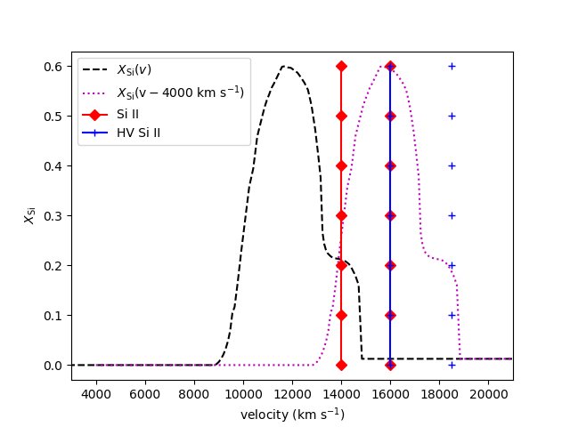
Figure A3: (a)

Figure A4: Comparison of the Si II distribution in W7 compared to the minimum and maximum PV and HV ion velocities in the day $+1$ SYNOW fit. When the W7 mass fraction function is shifted to the right by $4000$ $\text{km}~{}\text{s}^{-1}$, the distributions agree quite nicely. The red and blue markers denote min/max SYNOW velocities as in Figure 3

References

- Baron (2014) Baron, E. 2014, Nuclear Physics A, 928, 319
- Baron et al. (2006) Baron, E., Bongard, S., Branch, D., & Hauschildt, P. 2006, ApJ, 645, 480
- Benetti et al. (2005) Benetti, S., Cappellaro, E., Mazzali, P. A., et al. 2005, ApJ, 623, 1011
- Blondin et al. (2012) Blondin, S., et al. 2012, AJ, 143, 126
- Bongard et al. (2008) Bongard, S., Baron, E., Smadja, G., Branch, D., & Hauschildt, P. 2008, ApJ, 687, 456
- Branch (1998) Branch, D. 1998, Ann. Rev. Astr. Ap., 36, 37
- Branch (2001) —. 2001, PASP, 113, 169
- Branch et al. (2005) Branch, D., Baron, E., Hall, N., Melakayil, M., & Parrent, J. 2005, PASP, 117, 545
- Branch et al. (2009) Branch, D., Dang, L. C., & Baron, E. 2009, PASP, 121, 238
- Branch et al. (2006) Branch, D., Dang, L. C., Hall, N., et al. 2006, PASP, 118, 560
- Branch et al. (2007) Branch, D., et al. 2007, PASP, 119, 709
- Branch et al. (2008) Branch, D., Jeffery, D. J., Parrent, J., et al. 2008, PASP, 120, 135
- Candia et al. (2003) Candia, P., et al. 2003, PASP, 115, 277
- Childress et al. (2013) Childress, M., Aldering, G., Antilogus, P., et al. 2013, ApJ, 770, 108
- Contreras et al. (2018) Contreras, C., Phillips, M. M., Burns, C. R., et al. 2018, ApJ, 859, 24
- Fisher (2000) Fisher, A. 2000, PhD thesis, Univ. of Oklahoma, unpublished
- Hoeflich (2002) Hoeflich, P. 2002, New Astronomy Review, 46, 475
- Hoeflich et al. (2000) Hoeflich, P., Nomoto, K., Umeda, H., & Wheeler, J. C. 2000, ApJ, 528, 590
- Li et al. (2001) Li, W., et al. 2001, AJ, 113, 1178
- Marion et al. (2015) Marion, G. H., Sand, D. J., Hsiao, E. Y., et al. 2015, ApJ, 798, 39
- Nomoto et al. (1984) Nomoto, K., Thielemann, F.-K., & Yokoi, K. 1984, ApJ, 286, 644
- Nordin et al. (2011) Nordin, J., Östman, L., Goobar, A., et al. 2011, ApJ, 734, 42
- Phillips (1993) Phillips, M. M. 1993, ApJ, 413, L105
- Silverman et al. (2012) Silverman, J. M., Kong, J. J., & Filippenko, A. V. 2012, MNRAS, 425, 1819
- Silverman et al. (2013) Silverman, J. M., et al. 2013, MNRAS, 436, 1225
- Stritzinger et al. (2018) Stritzinger, M. D., Shappee, B. J., Piro, A. L., et al. 2018, ApJ, 864, L35
- Tripp (1998) Tripp, R. 1998, A&A, 331, 815
- Wang et al. (2009) Wang, X., Filippenko, A. V., Ganeshalingam, M., et al. 2009, ApJ, 699, L139
- Wang et al. (2012) Wang, X., et al. 2012, ApJ, 749, 126
- Zhang et al. (2014) Zhang, J.-J., Wang, X.-F., Bai, J.-M., et al. 2014, AJ, 148, 1