Freezing dynamics of entanglement and nonlocality for qutrit-qutrit ($3\otimes 3$) quantum systems

Abstract

We examine the possibilities of non-trivial phenomena of time-invariant entanglement and freezing dynamics of entanglement for qutrit-qutrit quantum systems. We find no evidence for time-invariant entanglement, however, we do observe that quantum states freeze their entanglement after decaying for some time. It is interesting that quantum states are changing whereas their entanglement remains constant. We find that the combined action of decoherence free subspaces and subspaces where quantum states decay, facilitate this phenomenon. This study is an extension of similar phenomena observed for qubit-qubit systems, qubit-qutrit, and multipartite quantum systems. We examine nonlocality of a specific family of states and find the certain instances where the states still remain entangled, however they can either loose their nonlocality at a finite time or remain nonlocal for all times.

I Introduction

Entanglement and nonlocality are two features of quantum mechanics which have attracted lot of interest and considerable efforts have been devoted to develop a theory of these phenomenona Horodecki-RMP-2009 ; gtreview . Due to growing efforts for experimental realizations of devices utilizing these features, it is essential to study the effects of noisy environments on entanglement and nonlocality. Such studies are an active area of research Aolita-review and several authors have studied decoherence effects on quantum correlations for both bipartite and multipartite systems Yu-work ; lifetime ; Aolita-PRL100-2008 ; bipartitedec ; Band-PRA72-2005 ; lowerbounds ; Lastra-PRA75-2007 ; Guehne-PRA78-2008 ; Lopez-PRL101-2008 ; Ali-work ; Weinstein-PRA85-2012 ; Ali-JPB-2014 ; Ali-2015 ; Ali-2016 ; Ali-2017 .

The specific noise dominant in experiments on trapped atoms is caused by intensity fluctuations of electromagnetic fields which leads to collective dephasing process. The dynamics of entanglement under collective dephasing has been studied for both bipartite and multipartite quantum systems Yu-CD-2002 ; AJ-JMO-2007 ; Li-EPJD-2007 ; Karpat-PLA375-2011 ; Liu-arXiv ; Carnio-PRL-2015 ; Carnio-NJP-2016 ; Song-PRA80-2009 ; Ali-PRA81-2010 . Some of these previous studies Ali-2017 ; Karpat-PLA375-2011 ; Liu-arXiv ; Carnio-PRL-2015 ; Carnio-NJP-2016 , revealed two interesting features of the dynamical process, which are so called freezing dynamics of entanglement Ali-2017 and time-invariant entanglement Karpat-PLA375-2011 ; Liu-arXiv ; Carnio-PRL-2015 ; Carnio-NJP-2016 . It was shown that a specific two qubits state may first decay upto some numerical value before suddenly stop decaying and maintain this stationary entanglement Carnio-PRL-2015 . Such behavior was also observed for various genuine multipartite specific states of three and four qubits, including random states Ali-2017 . Other interesting dynamical feature under collective dephasing is the possibility of time-invariant entanglement. Time-invariant entanglement does not necessarily mean that the quantum states live in decoherence free subspaces (DFS). In fact the quantum states may change at every instance whereas their entanglement remain constant throughout the dynamical process. This feature was first observed for qubit-qutrit systems Karpat-PLA375-2011 and more recently for qubit-qubit systems Liu-arXiv . We have investigated time-invariant phenomenon for genuine entanglement of three and four qubits. We have explicitly observed this phenomenon for a specific family of quantum states of four qubits Ali-2017 . For qutrit-qutrit ($3\otimes 3$) systems, some features of entanglement dynamics under collective dephasing are known, in particular the phenomenon of distillability sudden death Song-PRA80-2009 ; Ali-PRA81-2010 , however, so far to our knowledge, the possibility of time-invariant entanglement and freezing dynamics of entanglement has not been studied so far. In this work, we investigate these two features for this dimension of Hilbert space for a specific family of states and also for some random states.

Another aspect of quantum correlations is quantum nonlocality, which refers to the phenomenon that the predictions made using quantum mechanics cannot be simulated by a local hidden variable model. The existance of nonlocal correlations can be detected via violation of some types of Bell inequalities Bell-Phys-1964 . It is well known that pure entangled states violate a Bell inequality, whereas mixed entangled states may not do so Gisin-Werner-1991 . It is also known that entangled states do exhibit some kind of hidden nonlocality Liang-PRA86-2011 . The well known Clauser-Horne-Shimony-Holt (CHSH) inequality CHSH-1969 for two qubits has been studied under decoherence both in theory Mazzola-PRA81-2010 , and experiment Xu-PRL-2010 . Several investigations of nonlocality of multipartite quantum states under decoherence have been carried out NLD . The extension of CHSH inequality for multipartite quantum systems has received considerable attention in theory Mermin-PRL-1990 ; Ardehali-PRA-1992 ; Bancal-PRL-2011 ; Svetlichny-PRD-1987 ; Collins-PRL88-2002 ; Chen-PRA64-2001 and in experiments Pan-expMBI ; Bastian-PRL104-2010 . We have recently studied the effect of collective dephasing on genuine nonlocality of quantum states exhibiting time-invariant and freezing entanglement dynamics Ali-2017 . The problem of quantum nonlocality for high dimensional systems has been studied Kaszlikowski-PRL-2000 ; Kaszlikowski-PRA65-2002 ; Chen-PRA74-2006 . One particular inequality is called Collins-Gisin-Linden-Massar-Popescu (CGLMP) inequality CGLMP-PRL-2002 . In this work, we also study the effect of collective dephasing on nonlocality of qutrit-qutrit systems using CGLMP inequality.

This paper is organized as follows. In section II, we briefly discuss our model of interest. In section III, we review the idea of maximally entangled states for qutrit-qutrit systems and describe the method to compute a specific measure of entanglement for an arbitrary initial quantum state. We also review nonlocality and its computation in the same section. In section IV, we provide our main results. Finally, we conclude our work in section V.

II Collective dephasing for qutrit-qutrit systems

Our physical model consists of two qutrits (two three-level atoms for example) $A$ and $B$ that are coupled to a noisy environment, collectively. Our qutrits are sufficiently far apart and they do not interact with each other, so that we can treat them as independent. The collective dephasing refers to coupling of qutrits to the same noisy environment $B(t)$. The Hamiltonian of the quantum system (with $\hbar=1$) can be written as AJ-JMO-2007 ; Ali-PRA81-2010

$$H(t)=-\frac{\mu}{2}\,\big{[}\,B(t)(\sigma_{z}^{A}+\sigma_{z}^{B})\,\big{]}\,,$$ (1)

where $\mu$ is gyromagnetic ratio and $\sigma_{z}$ denotes the dephasing operator for qutrits $A$ and $B$. The stochastic magnetic fields refer to statistically independent classical Markov processes satisfying the conditions

$$\langle B(t)\,B(t^{\prime})\rangle = \frac{\Gamma}{\mu^{2}}\,\delta(t-t^{\prime})\,,$$

$$\langle B(t)\rangle = 0\,,$$ (2)

with $\langle\cdots\rangle$ as ensemble time average and $\Gamma$ denote the phase-damping rate for collective decoherence.

Let $|2\rangle$, $|1\rangle$, and $|0\rangle$ be the first excited state, second excited, and ground state of the qutrit, respectively. We choose the computational basis $\{\,|0,0\rangle$, $|0,1\rangle$, $|0,2\rangle\,|1,0\rangle$, $|1,1\rangle$, $|1,2\rangle$, $|2,0\rangle$, $|2,1\rangle$, $|2,2\rangle$,$\}$, where we have dropped the subscripts $A$ and $B$ with the understanding that first basis represents qutrit $A$ and second qutrit $B$. Also the notation $|0\rangle\otimes|0\rangle=|0\,0\rangle$ has been adopted for simplicity. The time-dependent density matrix for two-qutrits system is obtained by taking ensemble average over the noisy field, i. e., $\rho(t)=\langle\rho_{st}(t)\rangle$, where $\rho_{st}(t)=U(t)\rho(0)U^{\dagger}(t)$ and $U(t)=\exp[-\mathrm{i}\int_{0}^{t}\,dt^{\prime}\,H(t^{\prime})]$. The dynamics of density matrix can be given by operator sum representation AJ-JMO-2007 as $\rho(t)=\sum_{j}^{n}\,K_{j}^{\dagger}(t)\rho(0)K_{j}(t)$, where $K_{j}$ are Kraus operators that preserve the positivity and unit trace conditions, i. e., $\sum_{j}^{n}\,K_{j}^{\dagger}K_{j}=\mathbb{I}$. The most general solution of $\rho(t)$ under the assumption that the system is not initially correlated with environment is given as

$$\rho(t)=\,\sum_{k=1}^{3}\,(D_{k}^{AB\,\dagger}\,\rho(0)\,D_{k}^{AB})\,,$$ (3)

where the terms describing interaction with collective magnetic field $B(t)$ involve the operators $D_{1}^{AB}=\mathrm{diag}(\gamma(t),1,1,1,\gamma(t)\,,1,1,1,\gamma(t))$, $D_{2}^{AB}=\mathrm{diag}(\omega_{1}(t),0,0,0,\omega_{2}(t)\,,0,0,0,\omega_{2}(t))$, and $D_{3}^{AB}=\mathrm{diag}(0,0,0,0,\omega_{3}(t),0,0,0,\omega_{3}(t))$. The time dependent parameters are defined as, $\gamma=\mathrm{e}^{-\Gamma t/2}$, $\omega_{1}(t)=\sqrt{1-\gamma^{2}(t)}$, $\omega_{2}(t)=-\gamma^{2}(t)\,\sqrt{1-\gamma^{2}(t)}$, and $\omega_{3}(t)=(1-\gamma^{2}(t))\,\sqrt{1+\gamma^{2}(t)}$.

The matrix form of Eq. (3) for an arbitrary initial state is given as

$$\rho(t)=\left(\begin{array}[]{lllllllll}\rho_{11}&\gamma\rho_{12}&\gamma\rho_{13}&\gamma\rho_{14}&\gamma^{4}\rho_{15}&\gamma\rho_{16}&\gamma\rho_{17}&\gamma\rho_{18}&\gamma^{4}\rho_{19}\\ \gamma\rho_{21}&\rho_{22}&\rho_{23}&\rho_{24}&\gamma\rho_{25}&\rho_{26}&\rho_{27}&\rho_{28}&\gamma\rho_{29}\\ \gamma\rho_{31}&\rho_{32}&\rho_{33}&\rho_{34}&\gamma\rho_{35}&\rho_{36}&\rho_{37}&\rho_{38}&\gamma\rho_{39}\\ \gamma\rho_{41}&\rho_{42}&\rho_{43}&\rho_{44}&\gamma\rho_{45}&\rho_{46}&\rho_{47}&\rho_{48}&\gamma\rho_{49}\\ \gamma^{4}\rho_{51}&\gamma\rho_{52}&\gamma\rho_{53}&\gamma\rho_{54}&\rho_{55}&\gamma\rho_{56}&\gamma\rho_{57}&\gamma\rho_{58}&\rho_{59}\\ \gamma\rho_{61}&\rho_{62}&\rho_{63}&\rho_{64}&\gamma\rho_{65}&\rho_{66}&\rho_{67}&\rho_{68}&\gamma\rho_{69}\\ \gamma\rho_{71}&\rho_{72}&\rho_{73}&\rho_{74}&\gamma\rho_{75}&\rho_{76}&\rho_{77}&\rho_{78}&\gamma\rho_{79}\\ \gamma\rho_{81}&\rho_{82}&\rho_{83}&\rho_{84}&\gamma\rho_{85}&\rho_{86}&\rho_{87}&\rho_{88}&\gamma\rho_{89}\\ \gamma^{4}\rho_{91}&\gamma\rho_{92}&\gamma\rho_{93}&\gamma\rho_{94}&\rho_{95}&\gamma\rho_{96}&\gamma\rho_{97}&\gamma\rho_{98}&\rho_{99}\end{array}\right)\,.$$ (13)

We note that decoherence free subspaces (DFS) Yu-CD-2002 do appear in this system as a common characteristic of collective dephasing. Another interesting property of the dynamics is the fact that all initially zero matrix elements remain zero.

III Entanglement and nonlocality for $3\otimes 3$ quantum systems

In this section, we briefly review the key ideas and certain work related with entanglement and nonlocality for qutrit-qutrit systems. In subsection III.1, we discuss the maximally entangled states and a computable measures of entanglement. In subsection III.2, we review the nonlocality and methods to quantify it for quantum states.

III.1 Maximally entangled states of qutrit-qutrit systems

The analog of Bell-diagonal states of two qubits for qutrit-qutrit systems is simplex Baumgartner-PRA-2006 , which lives in nine dimensional real linear space. Let us consider the maximally entangled pure state, given as

$$|\Psi_{0,0}\rangle=\frac{1}{\sqrt{3}}\sum_{k=0}^{2}|k\rangle\otimes|k\rangle)\,.$$ (14)

We can construct the basis of $\mathbb{C}^{3}\otimes\mathbb{C}^{3}$ consisting of maximally entangled pure states, like Bell states as follows. Let $\mathbb{M}$ is set of indices $(m,n)$, where $m,n\in\mathbb{Z}_{3}$ with addition and multiplication of indices as modulo 3. For each pair $\lambda=(m,n)\in\mathbb{M}$, we can define a unitary operator

$$W_{\lambda}=W_{(m,n)}=\sum_{k=0}^{2}e^{\frac{2\,\pi\,i}{3}kn}\,|k\rangle\langle k+m|\,.$$ (15)

Then to each point $\lambda\in\mathbb{M}$, we associate the vector $|\Psi_{\lambda}\rangle\in\mathbb{C}^{3}\otimes\mathbb{C}^{3}$, as

$$|\Psi_{\lambda}\rangle=(W_{\lambda}\otimes\mathbb{I})\,|\Psi_{0,0}\rangle\,.$$ (16)

So we obtain the nine maximally entangled vectors, which form a basis of two qutrits vector space. We note that for collective dephasing model, six of these states reside in DFS and the rest of the 3 states reside in a space which is decoupled from DFS. While the geometry of Bell-diagonal states can be considered as tetrahedron with Bell states sitting at four corners, the corresponding geometry for qutrits is not that intuitive Baumgartner-PRA-2006 , however both cases contain the maximally mixed state “$\mathbb{I}/N^{2}$” at the center of tetrahedrons.

The problem of detection and quantification of entanglement for qutrit-qutrit systems is not an easy one. It is well know that for a given bipartite quantum state, if the matrix with a partial transpose taken with respect to either of the subsystem, has at least one negative eigenvalue, then the quantum state is entangled and called NPT state Peres-PRL-1996 . There exist some qutrit-qutrit quantum states which have positive partial transpose (PPT), nevertheless, they are entangled Horodecki-RMP-2009 ; Clarisse-PhD . These PPT-entangled states or so called bound entangled states (BES) pose the actual difficulty in order to characteristic and quantify entangled states. Although there are few criteria, like realignment criterion also called cross-norm criterion Chen-QIP-2003 to detect some of bound entangled states, nevertheless, in general the problem of detection of entanglement for this dimension of Hilbert space is not solved and it is an open issue.

Negativity Vidal-PRA65-2002 is a useful measure to quantify entanglement of bipartite NPT states, however, strictly speaking, this measure do not captures the bound entangled states, and for a given initial state, if negativity is zero, then it is not known in general whether the states are entangled or not except for isotropic states. In addition, as the dimension of Hilbert space for bipartite systems is larger than $4$ (qubit-qubit system), it is not always easy to find the analytical expressions for eigenvalues for an initial state. As negativity is quantified by adding negative eigenvalues, so exact expression for it is also intractable in many cases. Even the numerical computations could be done but the procedure is also not straightforward. The difficulty in computing the negativity numerically is now removed by recent studies in quantification of multipartite entanglement Bastian-PRL106-2011 . Although the main efforts of authors Bastian-PRL106-2011 were to quantify genuine entanglement for multipartite quantum systems, nevertheless, the genuine negativity simply gives the usual measure of negativity for bipartite quantum systems. We have used this measure in our study. The further details on computing this measure can be found in original work Bastian-PRL106-2011 .

III.2 Quantum nonlocality for qutrits

For a brief description of bipartite nonlocality, consider that each party can perform a measurement $X_{j}$ with result $a_{j}(b_{j})$ for $j=A(B)$. The joint probability distribution $P(a_{A}b_{B}|X_{A}X_{B})$ may exhibit different notions of nonlocality. It may be that it cannot be written in local form as

$$P(a_{A}b_{B}|X_{A}X_{B})=\int d\lambda P_{A}(a_{A}|X_{A}\lambda)\,P_{B}(b_{B}|X_{B}\lambda)\,,$$ (17)

where $\lambda$ is a shared local variable. Such nonlocality can be tested by standard Bell inequalities. One such inequality for two parties, two settings, and three outcomes is called CGLMP inequality CGLMP-PRL-2002 . The experimental violation of this inequality has been observed Vaziri-PRL-2002 as well. The inequality is given as

$$P(a=b)+P(b=a^{\prime}+1)+P(a^{\prime}=b^{\prime})$$

$$+P(b^{\prime}=a)-P(a=b-1)-P(b=a^{\prime})$$

$$-P(a^{\prime}=b^{\prime}-1)-P(b^{\prime}=a-1)\leq 2\,,$$ (18)

where the outcomes are $0,1,2$ and sum inside probabilities are modulo 3. The Bell operator associated with this inequality can be written Alsina-PRA94-2016 as

$$\mathcal{B}=2-3(a^{2}+b^{\prime 2})+\frac{3}{4}(ab+a^{2}b-a^{\prime}b-a^{\prime 2}b$$

$$-ab^{2}+a^{\prime}b^{2}+ab^{\prime}-a^{2}b^{\prime}+a^{\prime}b^{\prime}+a^{\prime 2}b^{\prime}+ab^{\prime 2}$$

$$-a^{\prime}b^{\prime 2})+\frac{9}{4}(a^{2}b^{2}-a^{\prime 2}b^{2}+a^{2}b^{\prime 2}+a^{\prime 2}b^{\prime 2})\,,$$ (19)

where we have omitted the tensor product symbols. The optimal measurements can be expressed in terms of eight Gell-Mann matrices. In general the exact form of these measurements are initial state dependent. However for an initial entangled state of the form $|\Psi_{0,0}\rangle$, the Bell operator Acin-PRA65-2002 is given as

$$\mathcal{B}=\left(\begin{array}[]{lllllllll}0&0&0&0&\frac{2}{\sqrt{3}}&0&0&0&2\\ 0&0&0&0&0&\frac{2}{\sqrt{3}}&0&0&0\\ 0&0&0&0&0&0&0&0&0\\ 0&0&0&0&0&0&0&\frac{2}{\sqrt{3}}&0\\ \frac{2}{\sqrt{3}}&0&0&0&0&0&0&0&\frac{2}{\sqrt{3}}\\ 0&\frac{2}{\sqrt{3}}&0&0&0&0&0&0&0\\ 0&0&0&0&0&0&0&0&0\\ 0&0&0&\frac{2}{\sqrt{3}}&0&0&0&0&0\\ 2&0&0&0&\frac{2}{\sqrt{3}}&0&0&0&0\\ \end{array}\right)\,.$$ (29)

It is well known that entangled qutrits violate local realism more stronger than qubits Kaszlikowski-PRL-2000 . For qubits, the maximum violation is achieved by Bell states and it is equal to $2\,\sqrt{2}\approx 2.8284$, whereas for qutrits the violation by maximally entangled state is equal to $\approx 2.8729$ Acin-PRA65-2002 . Surprisingly, it was found that the maximum violation for two qutrits is not achieved by maximally entangled state but by a non-maximally entangled state Acin-PRA65-2002 given as

$$|\psi_{\mu}\rangle=\frac{1}{\sqrt{2+\mu^{2}}}\,(|00\rangle+\mu|11\rangle+|22\rangle)\,,$$ (30)

with $\mu=(\sqrt{11}-\sqrt{3})/2\approx 0.7923$. It is not difficult to check that

$$\langle\,\mathcal{B}\,\rangle_{|\psi_{\mu}\rangle\langle\psi_{\mu}|}=\frac{12+8\sqrt{3}\mu}{6+3\mu^{2}}\,,$$ (31)

which is equal to $\langle\,\mathcal{B}\,\rangle\approx 2.9149$ for $\mu\approx 0.7923$. Similarly, for another entangled state Acin-PRL-2005

$$|\psi_{\nu}\rangle=\nu(|00\rangle+|11\rangle)+\sqrt{1-2\nu^{2}}|22\rangle)\,,$$ (32)

where $0\leq\nu\leq 1/\sqrt{2}$, the expectation value of Bell operator is given as

$$\langle\,\mathcal{B}\,\rangle_{|\psi_{\nu}\rangle\langle\psi_{\nu}|}=\frac{4\,\nu\,\big{(}\sqrt{3}\,\nu+(3+\sqrt{3})\sqrt{1-2\,\nu^{2}}\,\big{)}}{3}\,,$$ (33)

which achieve its maximum violation for $\nu\approx 0.617$ Acin-PRL-2005 .

IV Dynamics of entanglement and nonlocality

All previous studies Karpat-PLA375-2011 ; Liu-arXiv ; Carnio-PRL-2015 ; Carnio-NJP-2016 ; Ali-2017 which reported the possibility of time-invariant entanglement and freezing dynamics of entanglement have one fact common in their findings. The quantum states exhibiting these features are always mixtures of two entangled states and one of this entangled state reside in DFS such that when the entangled state living in subspace which is not decoherence free, decays, then somehow the entanglement present in DFS shields the combined states to preserve their entanglement. So, it is interesting to note that although quantum states (their eigenvalues as well) are changing all the time, nevertheless their entanglement remains stationary. In current system of two qutrits, we must also take a mixture of states from each subspace to check the possibility of time-invariant or freezing entanglement. To this aim, we define our initial states by mixing two entangled states from two decoupled subspaces. First let us consider the states,

$$\rho_{\alpha}=\alpha|\Psi_{0,0}\rangle\langle\Psi_{0,0}|+\frac{1-\alpha}{9}\,\mathbb{I}_{9}\,,$$ (34)

where $0\leq\alpha\leq 1$. These states are called isotropic states and they have the property that their PPT region is separable Clarisse-PhD . The states are NPT for $1/4<\alpha\leq 1$, and hence entangled. These states exhibit nonlocality for $\alpha>9/(2(3+2\sqrt{3}))\approx 0.6962$ Acin-PRA65-2002 . We now take another maximally entangled state residing in DFS, given as

$$|\Psi_{0,2}\rangle=\frac{1}{\sqrt{3}}\,\big{(}|02\rangle+|10\rangle+|21\rangle\,\big{)}\,.$$ (35)

This state is obtained using the relation (16). We can now define a family of states, which are mixture of isotropic states and $|\Psi_{0,2}\rangle$, given as

$$\rho_{\alpha,\beta}=\beta\,|\Psi_{0,2}\rangle\langle\Psi_{0,2}|+(1-\beta)\,\rho_{\alpha}\,,$$ (36)

where $0\leq\beta\leq 1$. Although, the entanglement properties for this family of states may not be very clear, however, the spectrum of states do shed some light on their being NPT or PPT. The partial transpose w.r.t. subsystem $B$ gives $9$ eigenvalues and $6$ of them are definitely positive for the given range of parameters $\alpha$ and $\beta$. The $3$ possible negative eigenvalues are all same and given as

$$\frac{1}{9}\,\big{[}(1-\alpha)(1-\beta)-3\sqrt{\alpha^{2}(1-\beta)^{2}-\alpha\beta(1-\beta)+\beta^{2}}\big{]}\,.$$ (37)

It is not difficult to check that for $\beta>1/4$, the states are NPT for $0\leq\alpha\leq 1$. Alternatively, the states are again NPT if $\alpha>0.277$ and $0\leq\beta\leq 1$.

The time evolution of these states follows from Eq. (13) and can be written as

$$\rho_{\alpha,\beta}(t)=\beta\,|\Psi_{0,2}\rangle\langle\Psi_{0,2}|+(1-\beta)\,\rho_{\alpha}(t)\,.$$ (38)

Hence $\rho_{\alpha}(t)$ decays, whereas $|\Psi_{0,2}\rangle$ remain dynamically invariant as it lives in DFS. Now there is an additional parameter $\Gamma t$ involved in the density matrix and due to this parameter not all the eigenvalues of partially transposed matrix are tractable. However, an interesting observation is accessible, which is the fact that out of three possible negative eigenvalues (given in Eq. (37)), one eigenvalue remains same and independent of parameter $\Gamma t$. This simply implies that if we choose the parameters $\alpha>0.277$ and $\beta>1/4$, the time evolved density matrix $\rho_{\alpha,\beta}(t)$ remain NPT for all the time and hence remain entangled. The other two negative eigenvalues become unknown functions of parameters $(\alpha,\,\beta,\,\Gamma t)$ and do feed (vary) any reasonable measure of entanglement, like negativity for some time until their contribution becomes extremely small or zero.

Another observation in previous studies on time-invariant and freezing dynamics of entanglement is the fact that the fraction of states living in DFS must always be larger than other state. This makes sense as if the state living in decaying subspaces has larger probability in the mixture then due to decoherence of this fraction, entanglement is expected to decay faster. On the other hand if the state living in DFS has a larger fraction then its share of entanglement in combined state would also be larger and more stable. So only in these situations, one can expect either time-invariant entanglement or its freezing dynamics. This is exactly the expected dynamics which have found in Figure (1). Although, we have included a very tiny fraction of states living outside decoherence free subspaces, nevertheless the entanglement does not remain invariant and decays with a very small rate (in 7th place after decimal point.). This simple example indicates that actually there is no time-invariant entanglement for this dimension of Hilbert space. However, we do expect the freezing dynamics of entanglement as the curve tends towards value $0.9985$.

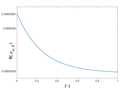
Figure 1: Entanglement monotone (negativity) for an initial state $\rho_{\alpha,\beta}(t)$ with parameters $\alpha=0.999$ and $\beta=0.999$. It can be seen that despite quite a very large fraction of states living in DFS, entanglement decays with an extremly small rate. See text for explanations.

In order to get a general trend of decay for an arbitrary initial states, we have generated $100$ random pure qutrit-qutrit states acoording to Haar measure Toth-CPC-2008 . We let these states interact with our reservoirs and we have studied their entanglement properties over a period of time. Figure (2) shows the results where it can seen that all of the initial NPT states remain NPT throughout the dynamical process. After initial entanglement decay upto a certain value, we observe the freezing behavior as expected. As all the off-diagonal elements living in DFS do not decay, so these elements in DFS retain their entanglement.

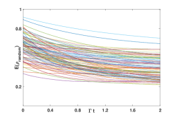
Figure 2: Entanglement monotone (negativity) is plotted against parameter $\Gamma t)$ for $100$ initial random pure states. It can be seen that all states remain NPT and more or less approach to a fixed (freezing) value of entanglement after some time.

Finally, we study the CGLMP inequality for this state $\rho_{\alpha,\beta}(t)$. For this aim, we need an appropriate Bell operator which depends on the type of initial state we want to test. If we choose our parameters such that the off-diagonal term for DFS is larger than we need to apply unitary transformation to operator $\mathcal{B}$ (Eq. (29)) before taking the expectation value of it, that is,

$$\tilde{\mathcal{B}}=(W_{0,2}\otimes\mathbb{I})\,\mathcal{B}\,(W_{0,2}^{\dagger}\otimes\mathbb{I})\,,$$ (39)

where $W_{0,2}$ is the unitary operator to get state $|\Psi_{0,2}\rangle$ from state $|\Psi_{0,0}\rangle$. It is straightforward to calculate the expectation value of this operator, which is given as

$$\langle\,\tilde{\mathcal{B}}\,\rangle_{\rho_{\alpha,\beta}(t)}=\frac{4\,\big{(}\sqrt{3}\,\alpha\,(1-\beta)\,e^{-2\,\Gamma t}+(3+2\,\sqrt{3})\beta\,\big{)}}{9}\,.$$ (40)

It is clear that for $\beta=1$, the state is trivially time-invariant (as it lives in DFS) and we have violation of $4(3+2\sqrt{3})/9\approx 2.8729$, for maximally entangled state $|\Psi_{0,2}\rangle$. For all values $\beta<1$, we have some change in nonlocality of quantum states, however for $\beta>9/(2(3+2\sqrt{3}))\approx 0.6961$ (This value coincides with the maximum white noise tolerance as discussed above), we have nonlocal asymptotic states and there is no so called sudden death of nonlocality.

Hence, we have both situations depending on parameter $\beta$, one with sudden death of quantum nonlocality but quantum states are still entangled and other case where states remain nonlocal and entangled.

V Conclusions

We have studied the behavior of bipartite entanglement under Markovian collective dephasing. Using a computable entanglement monotone, we have observed the freezing dynamics of entanglement which has not been studied before for qutrit-qutrit quantum systems. We have analyzed the dynamics of ensemble of random pure quantum states of two qutrits and have found that all of them remain NPT and hence entangled for all times. The specific family of states which we have studied, also exhibit freezing entanglement phenomenon. Depending on parameter $\beta$, the dynamics can be different. We have also examined quantum nonlocality for these states and it turned out that again depending upon parameter $\beta$, the initial states either loose their nonlocality at a finite time for $\beta<0.6961$ or remain nonlocal throughout the dynamics for $\beta$ larger than this value. In both of these cases, provided that $\beta>1/4$, the states remain NPT, means entangled irrespective of whether they are nonlocal or not. We have found no evidence for time-invariant entanglement for qutrit-qutrit states and based on our results, we conjecture that under current dynamics, this feature of time-invariant entanglement may not exist for qutrit-qutrit systems.

References

- (1) R. Horodecki et al., Rev. Mod. Phys. 81, 865 (2009).
- (2) O. Gühne and G. Tóth, Phys. Rep. 474, 1 (2009).
- (3) L. Aolita, F. de Melo, and L. Davidovich, Rep. Prog. Phys. 78, 042001 (2015).
- (4) T. Yu and J. H. Eberly, Phys. Rev. B 66, 193306 (2002); T. Yu and J. H. Eberly, Phys. Rev. B 68, 165322 (2003); T. Yu and J. H. Eberly, Phys. Rev. Lett. 93, 140404 (2004).
- (5) W. Dür and H.J. Briegel, Phys. Rev. Lett. 92, 180403 (2004); M. Hein, W. Dür, and H.-J. Briegel, Phys. Rev. A 71, 032350 (2005).
- (6) L. Aolita et al., Phys. Rev. Lett. 100, 080501 (2008).
- (7) C. Simon and J. Kempe, Phys. Rev. A 65, 052327 (2002); A. Borras et al., Phys. Rev. A 79, 022108 (2009); D. Cavalcanti et al., Phys. Rev. Lett. 103, 030502 (2009).
- (8) S. Bandyopadhyay and D. A. Lidar, Phys. Rev. A 72, 042339 (2005); R. Chaves and L. Davidovich, Phys. Rev. A 82, 052308 (2010); L. Aolita et al., Phys. Rev. A 82, 032317 (2010).
- (9) A. R. R. Carvalho, F. Mintert, and A. Buchleitner, Phys. Rev. Lett. 93, 230501 (2004).
- (10) F. Lastra, G. Romero, C. E. Lopez, M. França Santos and J. C. Retamal, Phys. Rev A 75, 062324 (2007).
- (11) O. Gühne, F. Bodoky, and M. Blaauboer, Phys. Rev. A 78, 060301(R) (2008).
- (12) C. E. López, G. Romero, F. Lastra, E. Solano, and J. C. Retamal, Phys. Rev. Lett. 101, 080503 (2008).
- (13) A. R. P. Rau, M. Ali and G. Alber, EPL 82, 40002 (2008); M. Ali, G. Alber, and A. R. P. Rau, J. Phys. B: At. Mol. Opt. Phys. 42, 025501 (2009); M. Ali, J. Phys. B: At. Mol. Opt. Phys. 43, 045504 (2010);
- (14) Y.S. Weinstein et al., Phys. Rev. A 85, 032324 (2012); S. N. Filippov, A. A. Melnikov, and M. Ziman, Phys. Rev. A 88, 062328 (2013).
- (15) M. Ali and O. Gühne, J. Phys. B: At. Mol. Opt. Phys. 47, 055503 (2014); M. Ali, Phys. Lett. A 378, 2048 (2014); M. Ali and A. R. P. Rau, Phys. Rev. A 90, 042330 (2014); M. Ali, Open. Sys. & Info. Dyn. Vol. 21, No. 4, 1450008 (2014).
- (16) M. Ali, Chin. Phys. B, Vol. 24, No. 12, 120303 (2015); M. Ali, Chin. Phys. Lett. Vol. 32, No. 6, 060302 (2015).
- (17) M. Ali, Int. J. Quant. Info. Vol.14, No. 7, 1650039 (2016).
- (18) M. Ali, Int. J. Quant. Info. Vol.15, No. 3, 1750022 (2017); M. Ali, Eur. Phys. J. D 71: 1 (2017).
- (19) T. Yu and J. H. Eberly, Phys. Rev. B 66, 193306 (2002); T. Yu and J. H. Eberly, Phys. Rev. B 68, 165322 (2003); T. Yu and J. H. Eberly, Optics Communications 264, 393 (2006).
- (20) G. Jaeger and K. Ann, J. Mod. Opt. 54(16), 2327 (2007).
- (21) Li S-B. and Xu J-B., Eur. Phys. J. D., 41, 377 (2007).
- (22) G. Karpat and Z. Gedik, Phys. Lett. A 375, 4166 (2011).
- (23) Liu B-H. et al., Phys. Rev. A 94 (2016) 062107.
- (24) Carnio E. G., Buchleitner A. and Gessner M., Phys. Rev. Lett. 115, (2015), 010404.
- (25) Carnio E. G., Buchleitner A. and Gessner M., New. J. Phys., 18, 073010 (2016).
- (26) W. Song, L. Chen, and S. L. Zhu, Phys. Rev. A 80, 012331 (2009).
- (27) M. Ali, Phys. Rev. A 81, 042303 (2010).
- (28) Bell J. S., Physics 1, 195 (1964).
- (29) Gisin N., Phys. Lett. A 154 (1991) 201; Werner R. F., Phys. Rev. A 40 (1989) 4277.
- (30) Liang Y-C., Masanes L. and Rosset D., Phys. Rev. A 86 (2011) 052115.
- (31) Clauser J. F., Horne M. A., Shimony A. and Holt R. A., Phys. Rev. Lett. 23 (1969) 880.
- (32) Mazzola L., Bellomo B., Lo Franco R. and Compagno G., Phys. Rev. A 81 (2010) 052116.
- (33) Xu J-S. et al., Phys. Rev. Lett. 104 (2010) 100502.
- (34) Laskowski W., Paterek T., Brukner C. and Zukowski M. Phys. Rev. A 81 (2010) 042101; Chaves R., Cavalcanti D., Aolita L. and Acin A., Phys. Rev. A 86 (2012) 012108; Chaves R., Acin A., Aolita L. and Cavalcanti D., Phys. Rev. A 89 (2014) 042106; Sohbi A., Zaquine I., Diamanti E. and Markham D., Phys. Rev. A 91 (2015) 022101; Divianszky P., Trencsenyi R., Bene E. and Vertesi T., Phys. Rev. A 93 (2016) 042113; Laskowski W., Vertesi T. and Wiesniak M., J. Phys. A: Math. Theor. 48 (2015) 465301.
- (35) Mermin D., Phys. Rev Lett. 65 (1990) 1838.
- (36) Ardehali M., Phys. Rev. A 46 (1992) 5375.
- (37) Bancal J-D., Brunner N., Gisin N. and Liang Y-C., Phys. Rev. Lett. 106 (2011) 020405.
- (38) Svetlichny G., Phys. Rev. D 35 (1987) 3066.
- (39) Collins D., Gisin N., Popescu S., Roberts D. and Scarani V., Phys. Rev Lett. 88 (2002) 170405.
- (40) J-L. Chen, D. Kaszlikowski, L. C. Kwek, C. H. Oh, and M. Zukowski, Phys. Rev. A 64, 052109 (2001).
- (41) Pan J. W. et al., Nature 403 (2000) 515; Lavoie J., Kaltenbaek R. and Resch K. J., New. J. Phys. 11 (2009) 073051; Erwen C. et al., Nature Photonics 8 (2014) 292.
- (42) Jungnitsch B. et al., Phys. Rev. Lett. 104 (2010) 210401.
- (43) D. Kaszlikowski, P. Gnaciński, M. Zukowski, W. Miklaszewski, and A. Zeilinger, Phys.Rev. Lett. 85, 4418 (2000); T. Durt, D. Kaszlikowski, and M. Zukowski, Phys. Rev. A 64, 024101 (2001).
- (44) D. Kaszlikowski, L. C. Kwek, J-L. Chen, M. Zukowski, and C. H. Oh, Phys. Rev A 65, 032118 (2002); J-L. Chen, D. Kaszlikowski, L. C. Kwek, and C. H. Oh, Mod. Phys. Lett. A 17, 2231 (2002).
- (45) J-L. Chen, C. Wu, L. C. Kwek, C. H. Oh, and M-L. Ge, Phys. Rev. A 74, 032106 (2006).
- (46) D. Collins, N. Gisin, N. Linden, S. Massar, and S. Popescu, Phys. Rev. Lett. 88, 040404 (2002).
- (47) B. Baumgartner, B. C. Hiesmayr, and N. Narnhofer, Phys. Rev. A 74, 032327 (2006); Ł. Derkacz and L. Jakóbczyk, Phys. Rev. A 76, 042304 (2007).
- (48) A. Peres, Phys. Rev. Lett. 77, 1413 (1996).
- (49) L. Clarisse, PhD thesis, University of York, England. arXiv: quant-ph/0612072.
- (50) K. Chen and L. A. Wu, Quantum Inf. Comput. 3, 193 (2003); O. Rudolph, Quant. Info. Proc. 4, 219 (2005).
- (51) G. Vidal and R.F. Werner, Phys. Rev. A 65 032314 (2002).
- (52) B. Jungnitsch, T. Moroder, and O. Gühne, Phys. Rev. Lett. 106, 190502 (2011); L. Novo, T. Moroder, and O. Gühne, Phys. Rev. A 88, 012305 (2013); M. Hofmann, T. Moroder, and O. Gühne, J. Phys. A: Math. Theor. 47, 155301 (2014).
- (53) A. Vaziri, G. Weihs, and A. Zeilinger, Phys. Rev. Lett. 89, 240401 (2002).
- (54) D. Alsina, A. Cervera, D. Goyeneche, J. I. Latorre, and K. Zyczkowski, Phys. Rev. A 94, 032102 (2016).
- (55) A. Acin, T. Durt, N. Gisin, and J. I. Latorre, Phys. Rev. A 65, 052325 (2002).
- (56) A. Acin, R. Gill, and N. Gisin, Phys. Rev. Lett. 95, 210402 (2005).
- (57) G. Tóth, Comput. Phys. Comm. 179, 430 (2008).