Universal Property of the Housekeeping Entropy Production

Abstract

The entropy production of a nonequilibrium system with broken detailed balance is a random variable whose mean value is nonnegative. Among the total entropy production, the housekeeping entropy production is associated with the heat dissipation in maintaining a nonequilibrium steady state. We derive a Langevin-type stochastic differential equation for the housekeeping entropy production. The equation allows us to define a housekeeping entropic time $\tau$. Remarkably, it turns out that the probability distribution of the housekeeping entropy production at a fixed value of $\tau$ is given by the Gaussian distribution regardless of system details. The Gaussian distribution is universal for any systems, whether in the steady state or in the transient state, whether they are driven by time-independent or time-dependent driving forces. We demonstrate the universal distribution numerically for model systems.

I Introduction

Recent developments of stochastic thermodynamics have made it possible to investigate thermodynamic properties of small-sized nonequilibrium systems Seifert (2012). In stochastic thermodynamics, thermodynamic quantities are defined at the level of a single trajectory realized by stochastic dynamics Sekimoto (1998). Among them, the entropy production is of particular importance. The total entropy production consists of two contributions: change in the stochastic entropy of a system under consideration and the entropy production in the thermal environment surrounding the system Seifert (2005). The entropy production turns out to be a measure of the extent to which the time-reversal symmetry is broken Schnakenberg (1976); Lebowitz and Spohn (1999); Maes and Netočný (2003); Chun and Noh (2018).

The total entropy production is decomposed into two parts. A nonequilibrium steady state is accompanied by a heat dissipation resulting in an entropy production of the thermal environment. Such an entropy production to maintain a nonequilibrium steady state is called the housekeeping entropy production. The remaining part is called the excess entropy production Oono and Paniconi (1998); Hatano and Sasa (2001); Lee et al. (2013). While the housekeeping entropy production is associated with dissipation in a nonequilibrium steady state, the excess entropy production occurs due to extra dissipation during relaxation toward a steady state or transition between steady states. They are also interpreted as adiabatic and nonadiabatic parts, respectively, in the perspective of time-scale separation Esposito and Van den Broeck (2010).

The total entropy production exhibits intriguing universal properties. Recently, it was found that the probability distribution should satisfy the fluctuation theorem. It is a direct consequence of the relation between the total entropy production and the broken time-reversal symmetry of nonequilibrium system dynamics Lebowitz and Spohn (1999); Crooks (1999); Seifert (2005). The fluctuation theorem guarantees that the mean total entropy production should be nonnegative. Experimental results support the validity of the fluctuation theorem for various kinds of nonequilibrium systems Wang et al. (2002); Carberry et al. (2004); Wang et al. (2005); Wong et al. (2017). More recently, after a pioneering investigation of Barato and Seifert Barato and Seifert (2015), it was found that the thermodynamic currents should obey the universal inequality called the thermodynamic uncertainty relation Gingrich et al. (2016, 2017); Pietzonka et al. (2017); Horowitz and Gingrich (2017); Proesmans and Van den Broeck (2017); Dechant and Sasa (2018a, b). The inequality reveals a trade-off relation between the current fluctuation and the total entropy production in a nonequilibrium steady state. Besides, extreme-value statistics of the total entropy production Neri et al. (2017) and entropic bounds on currents based on the Cauchy-Schwarz inequality Dechant and Sasa (2018c) have been studied.

One of the most interesting recent investigations on the total entropy production in nonequilibrium steady state was performed by Pigolotti et al. Pigolotti et al. (2017). They derived a Langevin-type stochastic differential equation of the total entropy production. In the steady state, by introducing a so-called entropic time, the stochastic differential equation can be transformed into a universal form that does not depend on system details. As a consequence, the probability distribution of the total entropy production at a fixed entropic time is universally given by the Gaussian distribution. The mapping to the entropic time provides an elegant explanation for the origin of the universal properties of the total entropy production. However, it is limited to the steady state of nonequilibrium systems under time-independent driving forces Pigolotti et al. (2017). It raises a question whether the universal property can be found even in the transient state under the time-dependent driving forces. In this paper, we will show that the housekeeping entropy production has the universal property not only in the steady state but also in the transient state even under time-dependent driving forces.

This paper is organized as follows. In Sec. II, we introduce a broad class of nonequilibrium thermodynamic systems described by the overdamped Langevin equation, and derive a stochastic differential equation for the housekeeping entropy production. Using the stochastic differential equation, we show that the housekeeping entropy production follows the universal distribution in Sec. III. In Sec. IV, we present numerical results for the model systems to demonstrate the theoretical results. We summarize our results in Sec. V.

II Stochastic differential equation for the housekeeping entropy production

We consider a multi-dimensional overdamped Langevin system in thermal contact with a heat bath at temperature $T$. The configuration is described by the column vector $\bm{x}=(x_{1},\cdots,x_{d})^{\rm T}$ for position variable with the superscript ^T representing the transpose. The position variable may stand for the coordinates of a single particle in a $d$ dimensional space or those of $n$ particles in a $(d/n)$ dimensional space. The particle is applied to the force

$$\bm{F}(\bm{x},\bm{\lambda}(t),\bm{\kappa}(t))=-\bm{\nabla}_{\bm{x}}V(\bm{x},\bm{\lambda}(t))+\bm{f}(\bm{x},\bm{\kappa}(t)),$$ (1)

where the first term is a conservative force with a potential energy $V$ and the second term is a nonconservative force. Note that $\bm{\nabla}_{\bm{x}}=(\partial_{x_{1}},\cdots,\partial_{x_{d}})^{\rm T}$ denotes the gradient with respect to $\bm{x}$ and that the column vector notation is adopted for $\bm{F}$ and $\bm{f}$. In general, both forces may depend explicitly on time through sets of protocol parameters $\bm{\lambda}(t)\equiv\{\lambda_{1}(t),\cdots,\lambda_{p}(t)\}$ and $\bm{\kappa}(t)\equiv\{\kappa_{1}(t),\cdots,\kappa_{q}(t)\}$. The Langevin equation is given by

$$\dot{\bm{x}}(t)=\mathsf{M}\bm{F}(\bm{x}(t),\bm{\lambda}(t),\bm{\kappa}(t))+\bm{\xi}(t)$$ (2)

where $\mathsf{M}$ is the mobility matrix, $\bm{\xi}(t)=(\xi_{1}(t),\cdots,\xi_{d}(t))^{\rm T}$ is a Gaussian white noise satisfying $\langle\bm{\xi}(t)\rangle=0$ and $\langle\bm{\xi}(t)\bm{\xi}^{\rm T}(t^{\prime})\rangle=2\mathsf{D}\delta(t-t^{\prime})$ with a diffusion matrix $\mathsf{D}$. The mobility matrix and the diffusion matrix are symmetric and positive definite, and satisfy the Einstein relation $\mathsf{D}=T\mathsf{M}$ Risken (1996); Zwanzig (2001). They are assumed to be independent of $\bm{x}$ and $t$. We set the Boltzmann constant to unity throughout this paper. The Fokker-Planck equation corresponding to (2) is given by Risken (1996); Gardiner (2010)

$$\partial_{t}P(\bm{x},t;\bm{\lambda}(t),{\bm{\kappa}}(t))=-\bm{\nabla}_{\bm{x}}\cdot\bm{J}(\bm{x},t;\bm{\lambda}(t),{\bm{\kappa}}(t))$$ (3)

with the probability current

$$\bm{J}=\mathsf{M}\bm{F}P-\mathsf{D}\bm{\nabla}_{\bm{x}}P.$$ (4)

For the sake of brevity, we omit arguments of functions unless it causes confusion.

The total energy $E$ of an overdamped Langevin system is given solely by the potential energy. When the protocol $\bm{\lambda}$ changes over time, the potential energy also changes. We define the net work $W$ done on the system as the sum of the potential energy change due to the protocol change and the work done by the nonconservative force, i.e., $W(t)=\int_{0}^{t}dt^{\prime}\dot{W}(t^{\prime})$ with

$$\dot{W}=\sum_{\alpha=1}^{p}\dot{\lambda}_{\alpha}(\partial_{\lambda_{\alpha}}V)+\dot{\bm{x}}\circ\bm{f}.$$ (5)

The heat dissipation is given by $Q(t)=\int_{0}^{t}dt^{\prime}\dot{Q}(t^{\prime})$ with Sekimoto (1998)

$$\dot{Q}=\dot{\bm{x}}\circ\bm{F}.$$ (6)

The notation $\circ$ denotes the inner product in the Stratonovich sense Risken (1996); Gardiner (2010). The definitions of work and heat are consistent with the energy conservation law $\dot{E}=\dot{W}-\dot{Q}$.

The total entropy production $S_{\rm tot}(t)=S_{\rm sys}(t)+S_{\rm env}(t)$ consists of the change in the stochastic entropy of a system ($S_{\rm sys}(t))$ and the entropy production in the heat bath ($S_{\rm env}(t)$) Seifert (2005). The stochastic entropy is defined by $s(t)=-\ln P(\bm{x}(t),t;\bm{\lambda}(t),\bm{\kappa}(t))$, whose mean value is the Shannon entropy of the probability distribution function $P$ Seifert (2005). The change in the stochastic entropy is then given by $S_{\rm sys}(t)=s(t)-s(0)$. The environmental entropy production is given by the Clausius form $S_{\rm env}(t)=Q(t)/T$ Seifert (2005).

Recently, Pigolotti et al. derived a Langevin-type stochastic differential equation for the total entropy production Pigolotti et al. (2017). The resulting equation reveals the universal statistical property of the total entropy production in the nonequilibrium steady state. Due to the steady state condition, the theory applies only to systems driven by a time-independent force. We extend the theory in search for the universal property of general nonequilibrium systems even in the transient state under a time-dependent driving force.

The total entropy production can be divided into the housekeeping entropy production $S_{\rm hk}$ and the excess entropy production $S_{\rm ex}$. Each contribution satisfies the fluctuation theorem in the absence of an odd-parity variable, such as momentum, under the time reversal Esposito and Van den Broeck (2010); Spinney and Ford (2012); Lee et al. (2013). When the protocol parameters $\bm{\lambda}$ and $\bm{\kappa}$ are fixed to constant values, the system ultimately relaxes to the corresponding nonequilibrium steady state. Maintaining the steady state, the system constantly dissipates the heat into the heat bath and produces the entropy. Such a contribution is called the housekeeping entropy production, while the rest is called the excess entropy production. Among them, we focus on the housekeeping entropy production. We describe below how it is defined in the single trajectory level. For more details, we refer readers to e.g. Refs. Speck and Seifert (2005); Esposito and Van den Broeck (2010).

Suppose that the position variable evolves along a trajectory $\bm{x}_{0}\to\cdots\to\bm{x}_{j}\to\cdots\to\bm{x}_{N}$ with $\bm{x}_{j}=\bm{x}(t_{j}=jdt)$ and $dt=t/N$ while the protocols change as $\bm{\lambda}_{0}\to\cdots\to\bm{\lambda}_{j}\to\cdots\to\bm{\lambda}_{N}$ with $\bm{\lambda}_{j}=\bm{\lambda}(t_{j})$ and similarly for $\bm{\kappa}$. At each $t_{j}$, we can define the fictitious steady state distribution $P_{\rm ss}(\bm{x};\bm{\lambda}_{j},\bm{\kappa}_{j})$ to which the system would relax if the protocols were fixed to the values $\bm{\lambda}_{j}$ and $\bm{\kappa}_{j}$. It is given by the solution of $\partial_{t}P_{\rm ss}=-\bm{\nabla}_{\bm{x}}\cdot{\bm{J}}_{\rm ss}(\bm{x};\bm{\lambda},\bm{\kappa})=0$ where

$${\bm{J}}_{\rm ss}(\bm{x};\bm{\lambda},\bm{\kappa})=\mathsf{M}\bm{F}(\bm{x},\bm{\lambda},\bm{\kappa})P_{\rm ss}-\mathsf{D}\bm{\nabla}_{\bm{x}}P_{\rm ss}$$ (7)

is the probability current in the fictitious steady state to given $\bm{\lambda}$ and $\bm{\kappa}$. The housekeeping entropy production is defined as Esposito and Van den Broeck (2010)

$$S_{\rm hk}\simeq\sum_{j=0}^{N-1}\ln\left[\frac{P_{\rm ss}(\bm{x}_{j};\bm{\lambda}_{j},\bm{\kappa}_{j})\Pi(\bm{x}_{j}\to\bm{x}_{j+1};\bm{\lambda}_{j},\bm{\kappa}_{j})}{P_{\rm ss}(\bm{x}_{j+1};\bm{\lambda}_{j},\bm{\kappa}_{j})\Pi(\bm{x}_{j+1}\to\bm{x}_{j};\bm{\lambda}_{j},\bm{\kappa}_{j})}\right]$$ (8)

where $\Pi(\bm{x}\to\bm{x}^{\prime};\bm{\lambda},\bm{\kappa})$ denotes the probability density of a transition from $\bm{x}$ to $\bm{x}^{\prime}$ for given instant protocols $\bm{\lambda}$ and $\bm{\kappa}$. The equality in (8) becomes exact in the limit of $N\to\infty$ with a fixed $t=Ndt$. The argument of the logarithm is identically equal to unity when the transition rates satisfy the detailed balance. Thus, the housekeeping entropy production measures the extent to which the detailed balance is broken. For the Langevin system described by (2), the housekeeping entropy production is given by Speck and Seifert (2005)

$$S_{\rm hk}(t)=\int_{0}^{t}dt^{\prime}~{}\dot{\bm{x}}(t^{\prime})\circ\frac{\mathsf{D}^{-1}\bm{J}_{\rm ss}(\bm{x}(t^{\prime});\bm{\lambda}(t^{\prime}),\bm{\kappa}(t^{\prime}))}{P_{\rm ss}(\bm{x}(t^{\prime});\bm{\lambda}(t^{\prime}),\bm{\kappa}(t^{\prime}))}.$$ (9)

Using the expression (9) and the Langevin equation (2), one can obtain a Langevin-type stochastic differential equation for $S_{\rm hk}(t)$. First, we rewrite the expression for the housekeeping entropy production in terms of the Itô product instead of the Stratonovich product to obtain

$$\frac{dS_{\rm hk}}{dt}=\dot{\bm{x}}\cdot\frac{\mathsf{D}^{-1}\bm{J}_{\rm ss}}{P_{\rm ss}}+\bm{\nabla}_{\bm{x}}\cdot\left(\frac{\bm{J}_{\rm ss}}{P_{\rm ss}}\right).$$ (10)

Replacing $\dot{\bm{x}}$ with the right hand side of (2) and using the property $\bm{\nabla}_{\bm{x}}\cdot\bm{J}_{\rm ss}=0$ of $\bm{J}_{\rm ss}$ in (7), one obtains that

$$\frac{dS_{\rm hk}(t)}{dt}=v(\bm{x}(t),\bm{\lambda}(t),\bm{\kappa}(t))+\sqrt{2v(\bm{x}(t),\bm{\lambda}(t),\bm{\kappa}(t))}\xi_{\rm hk}(t)$$ (11)

where

$$v=\frac{\bm{J}_{\rm ss}\cdot(\mathsf{D}^{-1}\bm{J}_{\rm ss})}{P_{\rm ss}^{2}}$$ (12)

and $\xi_{\rm hk}(t)$ is the Gaussian white noise satisfying $\langle\xi_{\rm hk}(t)\rangle=0$ and $\langle\xi_{\rm hk}(t)\xi_{\rm hk}(t^{\prime})\rangle=\delta(t-t^{\prime})$. The noise term is equal to $\bm{J}_{\rm ss}\cdot(\mathsf{D}^{-1}\bm{\xi}(t))/P_{\rm ss}$ with the noise $\bm{\xi}(t)$ in the Langevin equation (2). It is a Gaussian white noise with the same statistical properties as $\sqrt{2v}\xi_{\rm hk}$. The inner product symbol  $\cdot$  involving noise indicates Itô product throughout this paper.

Equation (11) is the key result of this paper, from which one can discover the universal property of the housekeeping entropy production. Before proceeding further, it is worth comparing (11) with the corresponding equation for the total entropy production considered in Ref. Pigolotti et al. (2017). The latter has the similar form to (11) with an additional term $(-2\partial_{t}\ln P)$, where $v$ is defined in terms of the genuine probability distribution and the current $P$ and $\bm{J}$ instead of the fictitious steady state ones. In the steady state, which exists only when the protocols are time-independent constants, the additional term $(-2\partial_{t}\ln P)$ vanishes and the total entropy production satisfies (11) with the constant $\bm{\lambda}$ and $\bm{\kappa}$. This comparison suggests that the housekeeping entropy production should display the universal statistical property even in the transient state under time-dependent driving forces.

III Universal property of the housekeeping entropy production

In this section, we explore the universal property of the housekeeping entropy production. The universal property is guaranteed by the form of the differential equation (11). We will follow the analysis in Ref. Pigolotti et al. (2017) which was done for the total entropy production in the steady state.

The housekeeping entropy production is known to satisfy the integral fluctuation theorem $\left\langle e^{-S_{\rm hk}(t)}\right\rangle=1$ Hatano and Sasa (2001); Speck and Seifert (2005). It can be derived straightforwardly from the evolution equation (11). Consider a random variable $Y(t)\equiv e^{-S_{\rm hk}(t)}$ with $Y(0)=e^{-S_{\rm hk}(0)}=1$. It satisfies

$$\frac{dY}{dt}=-\sqrt{2v}Y(t)\xi_{\rm hk}(t).$$ (13)

The ensemble average of the right hand side is identically zero due to the Itô calculus. Therefore, one has that $\langle Y(t)\rangle=\langle Y(0)\rangle=1$ at any $t$, which proves the integral fluctuation theorem.

In Eq. (11), the housekeeping entropy production has the deterministic part $v$ and the stochastic part $\sqrt{2v}\xi_{\rm hk}$. Note that $v$ is deterministic in the sense that its value is fixed for a given position variable $\bm{x}$. Upon taking the ensemble average, the stochastic part $\langle\sqrt{2v}\xi_{\rm hk}\rangle$ vanishes in the Itô calculus. That is, the deterministic component $v$ determines the average rate of the housekeeping entropy production. Note that the deterministic part (12) is nonnegative. Thus, it is useful to define a housekeeping entropic time $\tau$:

$$\tau(t)=\int_{0}^{t}dt^{\prime}v(\bm{x}(t^{\prime}),\bm{\lambda}(t^{\prime}),\bm{\kappa}(t^{\prime})).$$ (14)

It is a random variable depending on the stochastic trajectory of the system, whose mean is the average housekeeping entropy production. Due to the nonnegativity of $v$, the relation (14) defines a one-to-one mapping between $t$ and $\tau$ for a given stochastic trajectory. Their differentials are related as

$$d\tau=v(\bm{x}(t),\bm{\lambda}(t),\bm{\kappa}(t))dt.$$ (15)

We now consider the evolution of $S_{\rm hk}$ in the housekeeping entropic time scale $\tau$. The differential form of (11) is written as

$$dS_{\rm hk}=vdt+d\mathcal{W}_{\rm hk}(t)$$ (16)

with the uncorrelated Gaussian distributed random variables $d\mathcal{W}_{\rm hk}(t)$ satisfying $\langle d\mathcal{W}_{\rm hk}\rangle=0$ and $\langle d\mathcal{W}_{\rm hk}^{2}\rangle=2vdt$. Combining (15) and (16), one obtains $dS_{\rm hk}=d\tau+\sqrt{2}d\tilde{\mathcal{W}}_{\rm hk}(\tau)$ with the uncorrelated Gaussian distributed random variables $d\tilde{\mathcal{W}}_{\rm hk}(\tau)$ satisfying $\langle d\tilde{\mathcal{W}}_{\rm hk}\rangle=0$ and $\langle d\tilde{\mathcal{W}}_{\rm hk}^{2}\rangle=d\tau$. Equivalently, we obtain the Langevin-type equation

$$\frac{dS_{\rm hk}(\tau)}{d\tau}=1+\sqrt{2}\eta(\tau),$$ (17)

where $\eta(\tau)$ is a Gaussian white noise satisfying $\langle\eta(\tau)\rangle=0$ and $\langle\eta(\tau)\eta(\tau^{\prime})\rangle=\delta(\tau-\tau^{\prime})$. Therefore, the probability distribution of the housekeeping entropy production for a given $\tau$ is given by the Gaussian distribution

$$P(S_{\rm hk}|\tau)=\frac{1}{\sqrt{4\pi\tau}}\exp\left[-\frac{(S_{\rm hk}-\tau)^{2}}{4\tau}\right].$$ (18)

We emphasize that that (17) and (18) are valid universally for any nonequilibrium systems described by the overdamped Langevin equation, irrespectively of system details. System-specific details matter for the mapping between $t$ and $\tau$. However, once the housekeeping entropic time scale is adopted, the housekeeping entropy production always follows the Gaussian distribution whether the system is in the steady state or a transient state.

It is worth asking whether the excess entropy production can also be universal after a random time transformation. We introduce a short-hand notation $\bm{u}\equiv\bm{J}/P$, which is decomposed into the sum of $\bm{u}_{\rm hk}\equiv\bm{J}_{\rm ss}/P_{\rm ss}$ and $\bm{u}_{\rm ex}\equiv\bm{u}-\bm{u}_{\rm hk}$. Subtracting (11) from the differential equation for the total entropy production Pigolotti et al. (2017), one can derive the differential equation for the excess entropy production $S_{\rm ex}=S_{\rm tot}-S_{\rm hk}$. It is given by

$$\frac{dS_{\rm ex}}{dt} =-2\partial_{t}\ln P-\left(\sum_{i=1}^{p}\dot{\lambda}_{i}\partial_{\lambda_{i}}\ln P+\sum_{i=1}^{q}\dot{\kappa}_{i}\partial_{\kappa_{i}}\ln P\right)$$

$$~{}~{}~{}+(2\bm{u}_{\rm hk}+\bm{u}_{\rm ex})\cdot\mathsf{D}^{-1}\bm{u}_{\rm ex}+\sqrt{2{\bm{u}_{\rm ex}\cdot\mathsf{D}^{-1}\bm{u}_{\rm ex}}}\xi_{\rm ex}$$

where $\xi_{\rm ex}$ is a Gaussian white noise satisfying $\langle\xi_{\rm ex}(t)\rangle=0$ and $\langle\xi_{\rm ex}(t)\xi_{\rm ex}(t^{\prime})\rangle=\delta(t-t^{\prime})$. The noise term is equal to $\bm{u}_{\rm ex}\cdot\mathsf{D}^{-1}\bm{\xi}$ with the same $\bm{\xi}$ of the Langevin equation (2). Evidently, there is no simple proportionality relation between the deterministic part and the noise variance even when the protocol parameters are time-independent. Thus, we conclude that only the housekeeping entropy production displays the universal property in the transient state.

Meditating on the similarity between (17) and the corresponding equation for $S_{\rm tot}$ in the steady state Pigolotti et al. (2017), one may suspect whether the housekeeping entropy production satisfies the thermodynamic uncertainty relation even in the transient regime. Integrating (11), one obtains $S_{\rm hk}(t)=\tau(t)+\int_{0}^{t}dt^{\prime}\sqrt{2v(t^{\prime})}\xi_{\rm hk}(t^{\prime})$, which yields that $\langle S_{\rm hk}(t)^{2}\rangle=\langle\tau(t)^{2}\rangle+2\langle\tau(t)\rangle+2\Upsilon(t)$ with $\Upsilon(t)=\int_{0}^{t}dt^{\prime}\int_{0}^{t}dt^{\prime\prime}\langle v(t^{\prime\prime})\sqrt{2v(t^{\prime})}\xi_{\rm hk}(t^{\prime})\rangle$. Thus, the Fano factor $\mathcal{F}[S_{\rm hk}(t)]=(\langle S_{\rm hk}^{2}(t)\rangle-\langle S_{\rm hk}(t)\rangle^{2})/\langle S_{\rm hk}(t)\rangle$ for the housekeeping entropy production is given by

$$\mathcal{F}[S_{\rm hk}(t)]=2+\mathcal{F}[\tau(t)]+\frac{2\Upsilon(t)}{\langle\tau(t)\rangle}$$ (19)

with $\mathcal{F}[\tau(t)]=(\langle\tau^{2}(t)\rangle-\langle\tau(t)\rangle^{2})/\langle\tau(t)\rangle$. Following the formalism of Ref. Pigolotti et al. (2017), one can show that $\Upsilon(t)$ is equal to zero identically when the system is in the steady state. Thus, one recovers the thermodynamic uncertainty relation $(\langle S_{\rm hk}^{2}(t)\rangle-\langle S_{\rm hk}(t)\rangle^{2})/\langle S_{\rm hk}(t)\rangle\geq 2$ in the steady state. In the transient state, however, (19) does not guarantee the inequality $\mathcal{F}[S_{\rm hk}(t)]\geq 2$ with or without time-dependent protocol parameters.

IV Numerical studies on model systems

We demonstrate the universal property of the housekeeping entropy production with numerical simulations. The probability distributions of $S_{\rm hk}$ are obtained numerically in the following way: (i) The initial configuration $\bm{x}$ at $t=0$ is drawn from an initial distribution $P_{\rm ini.}(\bm{x})$. (ii) The increments of $\bm{x}$, $\tau$, and $S_{\rm hk}$ are evaluated using the time-discretized equations of motion with $dt$. The Heun algorithm is adopted Greiner et al. (1988). We choose $dt=0.0001$ in simulations, which is small enough. Time-dependent protocol parameters are also updated. (iii) The data are collected when $t$ or $\tau$ reaches a target value. The simulations are repeated independently for $N_{\rm samples}$ times to construct the probability distribution.

First, we reconsider a model studied in Ref. Pigolotti et al. (2017). A particle diffuses in a one-dimensional ring under a triangular potential

$$V(x)=\begin{cases}V_{0}\left(\frac{x}{x^{*}}\right)&{\rm for}~{}0\leq x<x^{*},\\ V_{0}\left(\frac{1-x}{1-x^{*}}\right)&{\rm for}~{}x^{*}\leq x<1.\end{cases}$$ (20)

The periodic boundary condition ($x+1=x$) is applied. In addition to the conservative force $-\partial V(x)/\partial x$, an $x$-independent force $f$ is applied to drive the system into a nonequilibrium state. The whole system is embedded in a heat bath at temperature $T$. The Langevin equation is given by

$$\dot{x}(t)=\mu F(x(t))+\sqrt{2\mu T}\xi(t)$$ (21)

where $\mu$ is the mobility of the particle,

$$F(x)=\begin{cases}F_{A}\equiv f-\frac{V_{0}}{x^{*}}&{\rm for}~{}0\leq x<x^{*},\\ F_{B}\equiv f+\frac{V_{0}}{1-x^{*}}&{\rm for}~{}x^{*}\leq x<1\end{cases}$$ (22)

is the total force, and $\xi(t)$ is a Gaussian white noise satisfying $\langle\xi(t)\rangle=0$ and $\langle\xi(t)\xi(t^{\prime})\rangle=\delta(t-t^{\prime})$. The protocol parameters $\bm{\lambda}=\{V_{0},x^{*}\}$ and $\bm{\kappa}=\{f\}$ may change over time.

The steady state probability distribution for fixed parameters is given by

$$P_{\rm ss}(x)=\begin{cases}\alpha_{1}+\alpha_{2}e^{F_{A}x/T}&{\rm for}~{}0\leq x<x^{*},\\ \alpha_{3}+\alpha_{4}e^{F_{B}x/T}&{\rm for}~{}x^{*}\leq x<1,\end{cases}$$ (23)

where the explicit expressions for $\alpha_{i}=\alpha_{i}(V_{0},x^{*},f)$ are found in Ref. Pigolotti et al. (2017). The corresponding current $J_{\rm ss}=\mu F_{A}\alpha_{1}=\mu F_{B}\alpha_{2}$ is an $x$-independent constant. With these expressions, one is ready to calculate the housekeeping entropy production and the housekeeping entropic time. We choose $P_{\rm ini.}(x)=\delta(x)$ and $N_{\rm samples}=10^{6}$.

We present the probability distribution of the housekeeping entropy production in Fig. 1. We performed the numerical simulations for three different protocol parameter sets, in which one among $V_{0}$, $x^{*}$, and $f$ varies in time while the others are kept to be constant. First of all, Fig. 1(a) shows the distributions at a fixed housekeeping entropic time $\tau=0.1$. Despite the difference in the protocol parameters, the probability distributions follow the predicted Gaussian distribution (18) with $\tau=0.1$. For comparison, we also present the probability distributions at fixed $t=0.1$ in Fig. 1(b). The probability distributions depend on the protocol and clearly deviate from the universal Gaussian distribution. This example confirms the universal distribution of the housekeeping entropy production even in the transient systems.

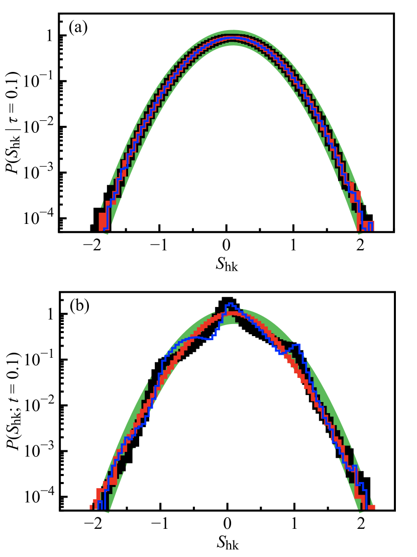
Figure 1: Probability distributions of the housekeeping entropy production (a) at fixed $\tau=0.1$ and (b) at fixed $t=0.1$. They were obtained from $N_{\rm samples}=10^{6}$ trajectories with $\mu=T=1$. Three different parameter sets are considered: (i) $x^{*}(t)=0.5+0.25\sin(20\pi t)$, $V_{0}=1$, and $f=1$ (black) (ii) $f(t)={\rm sign}(\sin(10\pi t))$, $V_{0}=1$, and $x^{*}=3/4$ (red) (iii) $V_{0}(t)=10t$, $x^{*}=3/4$, $f=1$ (blue). Also drawn is the Gaussian distribution in (18) with $\tau=0.1$ (green).

In order to highlight the difference of the housekeeping entropy production and the total entropy production, we next consider a two-dimensional Brownian motion under a harmonic potential $V(\bm{x})=\frac{1}{2}K(x_{1}^{2}+x_{2}^{2})$ in contact with a heat bath at temperature $T$. A linear nonconservative force $\bm{f}(\bm{x})=(\epsilon x_{2},-\epsilon x_{1})^{\rm T}$ drives the system into a nonequilibrium state. The parameter $\epsilon$ stands for the strength of the nonequilibrium driving. For simplicity, the mobility matrix is taken to be $\mathsf{M}=\mu\mathsf{I}$ with the identity matrix $\mathsf{I}$, and the initial distribution of $\bm{x}$ is taken be a Gaussian with zero mean and covariance $\sigma_{0}^{2}\mathsf{I}$. In this model, the protocol parameters $K$ and $\epsilon$ are taken to be time-independent.

The model belongs to the Ornstein-Uhlenbeck process Risken (1996), which is exactly solvable. The time-dependent probability distribution is given by

$$P(\bm{x},t)=\frac{1}{2\pi\sigma_{t}^{2}}\exp\left[-\frac{1}{2\sigma_{t}^{2}}\left(x_{1}^{2}+x_{2}^{2}\right)\right]$$ (24)

where $\sigma_{t}=\frac{T}{K}+e^{-2\mu Kt}\left(\sigma_{0}^{2}-\frac{T}{K}\right)$. The corresponding probability current is

$$\bm{J}(\bm{x},t)=\mu P(\bm{x},t)\begin{pmatrix}(\frac{T}{\sigma_{t}^{2}}-K)x_{1}+\epsilon x_{2}\\ -\epsilon x_{1}+(\frac{T}{\sigma_{t}^{2}}-K)x_{2}\end{pmatrix}.$$ (25)

The steady state probability distribution is given by $P_{\rm ss}(\bm{x})=\frac{K}{2\pi T}\exp[-\frac{K}{2T}(x_{1}^{2}+x_{2}^{2})]$ with the current $\bm{J}_{\rm ss}(\bm{x})=\mu\epsilon P_{\rm ss}(\bm{x})(x_{2},-x_{1})^{\rm T}$. Since the probability distribution in the transient state is available, one can measure the total entropy production $S_{\rm tot}(t)=[-\ln P(\bm{x}(t),t)+\ln P(\bm{x}(0),0)]+Q(t)/T$ as well as the housekeeping entropy production $S_{\rm hk}(t)$ numerically.

We present the numerical results for the total entropy production and the housekeeping entropy production in Fig. 2 with three different values of $K=4$, $6$, and $8$. Initially the system is prepared in the Gaussian distribution with $\sigma_{0}=0.1\neq\sigma_{\infty}\equiv\lim_{t\to\infty}\sigma_{t}$ so that the system is in a transient state. Then, $S_{\rm hk}$ is measured until $\tau=0.1$. Figure 2(a) shows that the housekeeping entropy production follows the same Gaussian distribution at all values of $K$ as predicted. In contrast, the total entropy production is known to be universal to a given value of the total entropic time $\tau_{\rm tot}$ only in the steady state Pigolotti et al. (2017). The total entropic time $\tau_{\rm tot}$ is defined by replacing $P_{\rm ss}$ and $J_{\rm ss}$ of $v$ in (14) with $P$ and $J$ Pigolotti et al. (2017). We also measured the total entropy production at $\tau_{\rm tot}=0.1$, whose probability distribution is presented in Fig. 2(b). The probability distributions of $S_{\rm tot}$ do not coincide with each other and do not have the Gaussian form. The time scale $\tau_{\rm tot}=0.1$ is too short for the system to relax into the steady state. This example demonstrates the universal fluctuations of the housekeeping entropy production in the transient state.

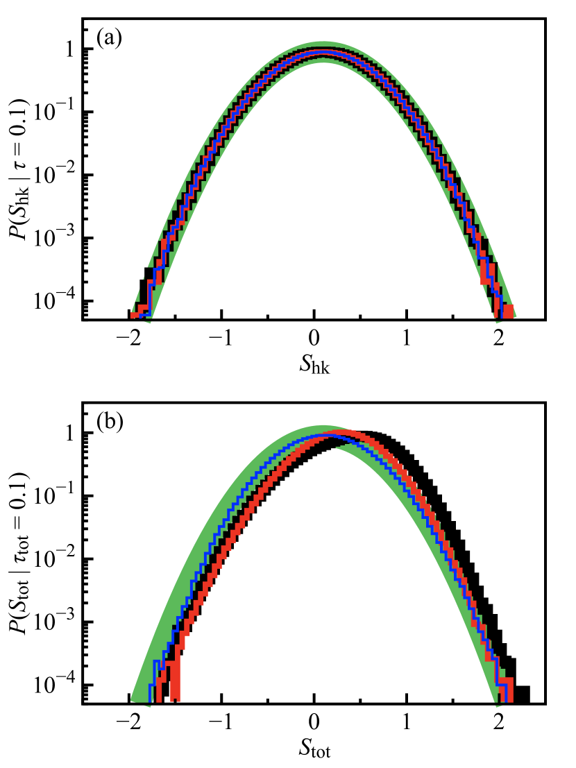
Figure 2: Probability distributions of (a) $S_{\rm hk}$ at fixed housekeeping entropic time $\tau=0.1$ and (b) $S_{\rm tot}$ at fixed total entropic time $\tau_{\rm tot}=0.1$. The parameters are $\mu=T=\epsilon=1$ and $K=$ 4 (black), 6 (red), and 8 (blue). The number of samples is $N_{\rm samples}=10^{6}$. Also shown is the Gaussian distribution in (18) with $\tau=0.1$ (green).

V Summary

We derived a Langevin-type stochastic differential equation of the housekeeping entropy production for a broad class of overdamped Langevin systems. The stochastic differential equation in (11) allows us to define the housekeeping entropic time $\tau$ as given in (14). The nonnegative contribution leads to define the housekeeping entropic time. We found that overdamped Langevin systems share the universal property regardless of system details: The housekeeping entropy production follows the Gaussian distribution in (18) for any systems on the entropic time scale. The universal property is confirmed by numerical simulations. Our study extends the work of Ref. Pigolotti et al. (2017) significantly. While the total entropy production displays the universal property only in the steady state under a time-independent protocols, the housekeeping entropy production does even in the transient state under a time-dependent protocol. We also remark that our formulation in (11) and (17) provides an easy understanding of the fluctuation theorem.

While most studies have focused on the universal property of the total entropy production, only a few studies have considered other thermodynamic quantities. It is noteworthy that Shiraishi et al. recently found a universal trade-off relation between the dynamical activity of a nonequilibrium system and the excess entropy production Shiraishi et al. (2018). Interestingly, similar to our results, a part of the total entropy production is shown to uncover a universal nature of nonequilibrium systems. These findings suggest that thermodynamic quantities other than the total entropy production can be useful in scrutinizing the universal properties of nonequilibrium systems. We hope that our study will promote the investigation of the universal properties of nonequilibrium systems not only in the steady state but also in the transient state.

References

- Seifert (2012) U. Seifert, Rep. Prog. Phys. 75, 126001 (2012).
- Sekimoto (1998) K. Sekimoto, Prog. Theor. Phys. Suppl. 130, 17 (1998).
- Seifert (2005) U. Seifert, Phys. Rev. Lett. 95, 040602 (2005).
- Schnakenberg (1976) J. Schnakenberg, Rev. Mod. Phys. 48, 571 (1976).
- Lebowitz and Spohn (1999) J. L. Lebowitz and H. Spohn, J. Stat. Phys. 95, 333 (1999).
- Maes and Netočný (2003) C. Maes and K. Netočný, J. Stat. Phys. 110, 269 (2003).
- Chun and Noh (2018) H.-M. Chun and J. D. Noh, J. Stat. Mech.: Theor. Exp. 2018, 023208 (2018).
- Oono and Paniconi (1998) Y. Oono and M. Paniconi, Prog. Theo. Phys. Suppl. 130, 29 (1998).
- Hatano and Sasa (2001) T. Hatano and S.-I. Sasa, Phys. Rev. Lett. 86, 3463 (2001).
- Lee et al. (2013) H. K. Lee, C. Kwon, and H. Park, Phys. Rev. Lett. 110, 050602 (2013).
- Esposito and Van den Broeck (2010) M. Esposito and C. Van den Broeck, Phys. Rev. Lett. 104, 090601 (2010).
- Crooks (1999) G. E. Crooks, Phys. Rev. E 60, 2721 (1999).
- Wang et al. (2002) G. M. Wang, E. M. Sevick, E. Mittag, D. J. Searles, and D. J. Evans, Phys. Rev. Lett. 89, 050601 (2002).
- Carberry et al. (2004) D. M. Carberry, J. C. Reid, G. M. Wang, E. M. Sevick, D. J. Searles, and D. J. Evans, Phys. Rev. Lett. 92, 140601 (2004).
- Wang et al. (2005) G. M. Wang, J. C. Reid, D. M. Carberry, D. R. M. Williams, E. M. Sevick, and D. J. Evans, Phys. Rev. E 71, 046142 (2005).
- Wong et al. (2017) C.-S. Wong, J. Goree, Z. Haralson, and B. Liu, Nature Physics 14, 21 (2017).
- Barato and Seifert (2015) A. C. Barato and U. Seifert, Phys. Rev. Lett. 114, 158101 (2015).
- Gingrich et al. (2016) T. R. Gingrich, J. M. Horowitz, N. Perunov, and J. England, Phys. Rev. Lett. 116, 120601 (2016).
- Gingrich et al. (2017) T. R. Gingrich, G. M. Rotskoff, and J. M. Horowitz, J. Phys. A 50, 184004 (2017).
- Pietzonka et al. (2017) P. Pietzonka, F. Ritort, and U. Seifert, Phys. Rev. E 96, 012101 (2017).
- Horowitz and Gingrich (2017) J. M. Horowitz and T. R. Gingrich, Phys. Rev. E 96, 020103 (2017).
- Proesmans and Van den Broeck (2017) K. Proesmans and C. Van den Broeck, Europhys. Lett. 119, 20001 (2017).
- Dechant and Sasa (2018a) A. Dechant and S.-I. Sasa, J. Stat. Mech.: Theor. Exp. 2018, 063209 (2018a).
- Dechant and Sasa (2018b) A. Dechant and S.-I. Sasa (2018b), eprint arXiv:1804.08250v2 [cond-mat.stat-mech].
- Neri et al. (2017) I. Neri, É. Roldán, and F. Jülicher, Phys. Rev. X 7, 011019 (2017).
- Dechant and Sasa (2018c) A. Dechant and S.-i. Sasa, Phys. Rev. E 97, 062101 (2018c).
- Pigolotti et al. (2017) S. Pigolotti, I. Neri, É. Roldán, and F. Jülicher, Phys. Rev. Lett. 119, 140604 (2017).
- Risken (1996) H. Risken, The Fokker-Planck Equation: Methods of Solution and Applications (Springer-Verlag, Berlin, 1996), 2nd ed.
- Zwanzig (2001) R. Zwanzig, Nonequilibrium Statistical Mechanics (Oxford University Press, New York, 2001).
- Gardiner (2010) C. Gardiner, Stochastic Methods: A Handbook for the Natural and Social Sciences (Springer, New York, 2010), 4th ed.
- Spinney and Ford (2012) R. E. Spinney and I. J. Ford, Phys. Rev. Lett. 108, 170603 (2012).
- Speck and Seifert (2005) T. Speck and U. Seifert, J. Phys. A 38, L581 (2005).
- Greiner et al. (1988) A. Greiner, W. Strittmatter, and J. Honerkamp, J. Stat. Phys. 51, 95 (1988).
- Shiraishi et al. (2018) N. Shiraishi, K. Funo, and K. Saito, Phys. Rev. Lett. 121, 070601 (2018).