A flexible sequential Monte Carlo algorithm for parametric constrained regression
Abstract
An algorithm is proposed that enables the imposition of shape constraints on regression curves, without requiring the constraints to be written as closed-form expressions, nor assuming the functional form of the loss function. This algorithm is based on Sequential Monte Carlo-Simulated Annealing and only relies on an indicator function that assesses whether or not the constraints are fulfilled, thus allowing the enforcement of various complex constraints by specifying an appropriate indicator function without altering other parts of the algorithm. The algorithm is illustrated by fitting rational function and B-spline regression models subject to a monotonicity constraint. An implementation of the algorithm using R is freely available on GitHub.
keywords:
shape constraints , constrained optimisation , simulated annealing , sequential Monte Carlo , rational functions , B-splines1 Introduction
Shape constraints, such as monotonicity or convexity, can be required on a regression curve to ensure its interpretability due to some external theory. For instance, growth curve modelling often requires monotonicity constraints to be imposed on the response curve (Marsh, 1980; Thornley, 1999), or shape constrained models can be used to estimate dose-response curves (Kelly and Rice, 1990), cumulative distribution functions (Ramsay, 1998) and various response curves in economics that are convex by some underlying theory (Matzkin, 1991). Therefore, fitting a shape-constrained regression model becomes a constrained optimisation problem, where the parameter space of the regression coefficients is appropriately restricted.
Despite the importance of restricting the shape of the regression curves, current shape constrained models are mainly concentrated on polynomial or spline models due to their relative ease of implementation. For instance, when considering monotonicity in polynomial models, apart from directly minimising the loss function subject to a restricted parameter space (Bon et al., 2017), such constraints can be achieved through an appropriate model parameterisation (Elphinstone, 1983; Murray et al., 2013, 2016; Manderson et al., 2017). On the other hand, when using penalised splines, the monotonicity or convexity conditions for models with truncated power bases (up to quadratic spline) or B-spline bases can be written as a system of linear inequality constraints (Leitenstorfer and Tutz, 2007; Brezger and Steiner, 2008; Hazelton and Turlach, 2011; Meyer et al., 2011; Meyer, 2012; Pya and Wood, 2015). However, shape-constrained models other than these are less common, partly due to the difficulty of deriving appropriate closed-form expressions required for enforcing the constraints. This motivates us to develop a flexible method that is capable of imposing shape constraints on a wide variety of regression models, even in the absence of closed-form expressions of the constraints.
We propose a new constrained optimisation method that works on any constraints that are presentable as an indicator function. Such constraints are not enforced by exploiting the mathematical expressions that describe them; rather, the feasibility of an estimate is only known from the indicator function. Consequently, our method is more versatile than those that assume specific structures on the constraints. To our knowledge, the only other optimisation method developed with the black-box constraint property is the Constrained Estimation Particle Swarm Optimisation (CEPSO, Wolters, 2012) algorithm. However, CEPSO requires a pilot estimate to operate, which is usually the unconstrained global minimum. Since the unconstrained global minimum is often difficult to obtain, especially when there are multiple local minima in the loss function, there are some circumstances when CEPSO may be unsuitable. Our method is based on Sequential Monte Carlo-Simulated Annealing (SMC-SA, Zhou and Chen, 2013), and will overcome the need for a pilot estimate.
The remainder of the paper is outlined as follows: In Section 2, we will formally define the optimisation problem and discuss the challenges of solving this. The details of the constraint-augmented SMC-SA are discussed in Section 3. In Section 4, the performance of our method will be assessed by fitting regression models on both simulated and real-world datasets. We conclude and discuss our algorithm in Section 5.
2 Problem specification
Constrained regression analysis is usually analogous to finding a state , where the feasible set is not necessarily finite or convex, such that a loss function is minimised
For the purpose of this study, we assume that is unique.
The classic approach of solving constrained optimisation problems is to introduce Lagrange multipliers into the loss function, and solve the system of equations attained from partially differentiating the transformed function with respect to the parameters and Lagrange multipliers (see for example Nocedal and Wright, 2006). In the usual case of minimising a complicated loss function, iterative algorithms may be the more sensible choice (see for example Romeijn and Smith, 1994; Andreani et al., 2013; Reddi et al., 2015).
However, most of the existing constrained optimisation methods are restricted to only solving problems with particular types of constraints, and are consequently not suitable for the development of a flexible constrained optimisation methodology. Moreover, there are constraints which cannot be written down as a finite set of closed-form expressions. For example, fitting a least squares continuous rational function requires its denominator polynomial to be non-zero over the region of interest, implying that there are infinitely many non-equalities to be considered. It is therefore difficult, if not impossible, to implement any of the traditional methods for this problem.
3 Optimisation
It is well known that the Boltzmann distribution of the form
will converge to a degenerate distribution whose mass is concentrated on the global minimum of when the temperature converges to 0. Similarly for constrained optimisation problems, it can be shown that this will still hold when the solution space is restricted. That is, the distribution
| (1) |
where is an indicator for , will converge to a degenerate distribution concentrated on the constrained global minimum (Romeijn and Smith, 1994). In light of these results, a constrained optimisation problem can essentially be solved by drawing samples from (1) with , a fact employed by the algorithm we propose.
3.1 Simulated annealing
The Metropolis algorithm (Metropolis et al., 1953), a Markov chain Monte Carlo (MCMC) technique, can be employed to draw samples from (1), in a similar fashion to simulated annealing (Kirkpatrick et al., 1983; Locatelli, 2000). More specifically, we sample from a sequence of Boltzmann distributions
| (2) |
that starts from a Boltzmann distribution with high temperature and eventually converges to the degenerate distribution of interest (i.e. ). Simulated annealing first simulates a Markov chain with invariant , then proceeds to simulate the rest of with fresh Markov chains using the sample from the preceding as starting states. This construction of sampling from a distribution sequence, rather than direct sampling from (1) with low , is necessary to facilitate efficient sampling due to the low acceptance probability of the Markov chain when the temperature is low. This can be observed evidently from the formula of the acceptance probability for each
| (3) |
where and denote proposed and previous states respectively. At low temperatures, even a small difference of will lead to the exponential function evaluating to a large negative value.
Since simulated annealing minimises by sampling from (2), there are two decisions to be made: the number of samples drawn from before moving to , and the choice of temperature at each iteration. Naturally when sampling from , the ideal situation will be simulating its corresponding Markov chain until the invariant distribution of the chain is achieved, and using the sample from as the starting state of the subsequent Markov chain to sample from . This strategy is clearly impractical in general due to the large amount of transitions required for each Markov chain to achieve stationarity; rather, the common practice is to perform only a single transition for each . Consequently, those Markov chains never achieve their stationarity, and some conditions (such as the choice of and the proposal distribution) have to be followed to ensure that the whole algorithm will still minimise when (Locatelli, 2000). For more detailed analysis and implementation of constrained simulated annealing with compact , we refer to Romeijn and Smith (1994) and Locatelli (2002).
While simulated annealing will converge to the global minimum when , in practice one can only carry out a finite number of iterations. This may lead the algorithm to converge to a local minimum if it starts from a poor state and stops prematurely. However, with the abundance of parallel computing power available nowadays, this issue can be mitigated by performing multiple independent simulated annealings that start from different states. For the rest of this paper, we will refer to this technique as multi-start SA, which starts from different locations, leading to the following set of search chains after iterations. Arguably, this strategy of starting from multiple states is widely used by practitioners when multiple local minima are present in the loss function, in the hope that at least one of the search chains will converge to the global minimum. As we will argue in the following, multi-start SA can be improved by utilising the information extracted from at each iteration, which is the motivation of SMC-SA.
3.2 Sequential Monte Carlo-Simulated Annealing
An alternative approach to sampling from (2) is the Sequential Monte Carlo (SMC) sampler proposed by Del Moral et al. (2006) and formalised by Zhou and Chen (2013), who then called the resulting algorithm Sequential Monte Carlo-Simulated Annealing (SMC-SA). Intuitively speaking, SMC-SA is a multi-start SA algorithm combined with the idea of importance sampling. Prior to the start of Markov transitions at each iteration, the importance sampling step will only select the states with lower loss function values for further optimisation, and discard the rest to save computational resources. From a MCMC perspective, all states are weighted and sampled at the start of each iteration to resemble before performing a Markov transition, such that the single-transition Markov chain can achieve its invariant distribution (i.e. ) more easily.
We will discuss SMC-SA as a two-step process, namely importance sampling and the SA-move.
-
1.
Importance sampling: The idea of the importance sampling step is to filter out states with greater loss function values, which are less likely to lead to the global minimum. This is implemented by sampling promising states from the pool of previous states at the start of each iteration, according to the weights assigned to each
(4) The eventual output from the importance sampling step is a set .
-
2.
SA-move (Markov kernel): The from the importance sampling step are then transitioned once with a Markov kernel with invariant distribution of . For each , a candidate state is drawn from a symmetrical random walk proposal which is centred on , and performs an accept-reject routine according to (3) to determine . This step is essentially performing an iteration of the Metropolis algorithm with as the starting state.
3.2.1 Proposal distribution
The selection of can greatly affect the transition of the chain, and thus the quality of the samples being drawn. More specifically, a proposal distribution with significant mass outside will result in the chain rarely moving to a new state, as (3) will evaluate to 0 when is not feasible. In this case, a random walk proposal with support , which we refer to as a truncated random walk for the remainder of this paper, will be a more ideal candidate than a symmetrical random walk as the acceptance probability will be strictly positive. Using a proposal other than a symmetrical random walk also implies that (3) needs to be adjusted with a ratio of proposal densities evaluated at the current and proposed states (Hastings, 1970)
| (5) |
to preserve the reversibility of the Markov kernel. However, the calculation of (5) is not trivial.
In light of the ratio of proposal distributions in (5) being intractable, we suggest ignoring this ratio and using (3) to calculate acceptance probabilities. This strategy is equivalent to having a Markov chain with a symmetrical random walk proposal and transitioning the chain until the acceptance probability is non-zero. A truncated random walk merely rejects the infeasible states at the proposal stage rather than at the acceptance-rejection stage. Although omitting the proposal ratio might result in the Markov chains having invariant distributions other than (2), we are not interested in estimating the density of the exact Boltzmann distributions, but rather the states that correspond to high density regions. The sequence of Boltzmann distributions is only a vehicle to minimise . Our aim can still be achieved as long as the global minimum is visited by the algorithm.
Sampling from a truncated random walk, especially when the nature of the constraint is unknown, is difficult and we usually have to use a rejection sampler. In our algorithm, we use a truncated Gaussian random walk proposal
| (6) |
This proposal can be generated with a rejection sampler, by repeatedly adding a -dimensional Gaussian noise to until a feasible is obtained.
When is high-dimensional, can be small relative to ; thus, a rejection sampler for (6) is notoriously inefficient. In this case, we suggest using a -point operator proposal, as shown in Liang et al. (2014), which updates only components of in each iteration. The components to be updated are randomly chosen at the beginning of the Markov transition, and a -dimensional Gaussian noise is repeatedly added to the chosen components until a feasible is obtained, as in the case where .
3.2.2 Cooling schedule
A cooling schedule is a function that controls the temperature at each iteration, which in turn affects the algorithm convergence. It should restrict the cooling rate such that the invariant distributions of adjacent Markov chains do not differ too much, and the initial states for each chain in (2) are more likely to fall within the high density region of their respective invariant distributions. The choice of cooling schedule is usually dependent on the problem at hand. However, in general, there are two conditions that need to be met for SMC-SA to converge: and is monotonically decreasing (Zhou and Chen, 2013). Schedules that satisfy both of these conditions include the logarithm schedule, which is suggested in Zhou and Chen (2013) and has the form
where is the best state observed up until the iteration. However, as described in Nourani and Andresen (1998), the cooling rate of the logarithm schedule can be too conservative, and an alternative is to use a more stringent reciprocal schedule
| (7) |
In our experience, this schedule outperforms the logarithm schedule when using our modified SMC-SA algorithm in terms of the best minimum achieved for a given number of iterations, despite not being monotonically decreasing.
3.2.3 SMC-SA and SMC sampler
The SMC-SA algorithm can also be seen as a special case of the SMC sampler (Del Moral et al., 2006) that simulates the distribution sequence in (2) with the following specifications:
-
1.
the initial distribution is ;
-
2.
Metropolis MCMC forward kernels are used with invariant distributions given by (2);
-
3.
the backward kernels are
-
4.
states are resampled after each iteration to avoid degeneracy.
In this case, (4) gives the weights for each sample in the SMC sampler. The implementation of is outlined in Algorithm 1.
3.3 Stochastic approximation annealing
Stochastic approximation annealing (SAA) is another improvement on the simulated annealing proposed by Liang et al. (2014). Rather than sampling from (2) directly, SAA partitions the parameter space into multiple regions according to their loss function values
where are arbitrary but fixed. SAA seeks to sample from the following sequence of partitioned Boltzmann distributions
| (8) |
which resembles a mixture of Boltzmann distributions truncated to . The extra hyperparameters , which vary at each iteration, control the mixing probability and are updated to encourage the exploration of partitions that are previously unvisited. Liang et al. (2014) proved that such augmentation on the Boltzmann distributions allows SAA to converge using a square-root schedule as opposed to the logarithm schedule used in standard simulated annealing, thus achieving a faster convergence rate.
In principle, we can further improve SAA by using an SMC sampler, instead of a Metropolis-Hastings sampler as suggested in the original implementation in Liang et al. (2014), to simulate the sequence (8). We conjuncture that the resulting algorithm will resemble the following structure in each iteration:
While SAA incorporated with a SMC sampler may converge faster, the convergence performance of SAA depends on the partition , which can be challenging to choose. In light of this issue, a detailed study of incorporating SAA into our algorithm is left for future research.
4 Applications
In this section, we will discuss the convergence performance of our augmented SMC-SA in a regression context. We demonstrate our algorithm by fitting rational function models and B-spline models, both of which are subject to monotonicity constraints. We use either a least squares estimator or Tukey’s biweight estimator, depending on the dataset. The results are then compared to that from multi-start SA and CEPSO, which will also serve as our benchmark. This simulation study was conducted in R (R Core Team, 2018) on an Intel Core i7-6700 (3.4GHz) machine with 8 gigabytes of RAM. The code for implementing the algorithm and simulation study is available on https://github.com/weiyaw/blackbox.
All of the algorithms which we tested require a set of starting states , rather than a single point in the parameter space, to operate efficiently. We ran all the algorithms 40 times, each of which started with different sets of 1000 states. The same set of starting states were used across different algorithms to ensure a fair comparison. The set of starting states are generated from the following procedure:
-
1.
Obtain a crude estimate ;
-
2.
Draw a sample from until that sample is feasible;
- 3.
A Cauchy distribution is preferred due to its heavy tails (Meyer, 2003), which allows the set of starting states to cover more areas in , although a uniform distribution is more suitable when is bounded.
We tried three different cooling schedules for SMC-SA: the logarithm schedule, and the reciprocal schedule with set to 0.85 and 0.95. For multi-start SA, we only used the logarithm schedule since the reciprocal schedule is too aggressive. The variance parameter in (6), the number of states and the number of iterations performed were then set according to the cooling schedule used in the algorithm and are given in Table 1. The was decreased after each iteration to allow a smaller step size and thus a finer improvement at the latter stages of the algorithm. We also used a 2-point operator proposal for all the examples, unless specified otherwise. The number of iterations was chosen to ensure that the computational efforts across different algorithms were roughly the same. In general, a more stringent cooling schedule requires less iterations but more samples to converge.
| Schedule | Iterations | ||
|---|---|---|---|
| Logarithm | 1000 | 3000 | |
| Reciprocal | 3000 | 1000 |
For CEPSO, the algorithm used 2000 iterations and the neighbourhood size for the local best estimation was set to 200. The methods used to obtain the pilot estimates are problem-specific and will be discussed later.
4.1 Rational function models
Rational functions are fractions whose numerator and denominator are both polynomials. They are usually more flexible than polynomials in the sense that they can describe a given curve with fewer parameters, yet retaining the same degree of accuracy (Newman, 1964; Ralston and Rabinowitz, 2001). Apart from their superior flexibility, some physical phenomena can be precisely modelled as a rational function, such as the Michaelis-Menten kinetics model in biochemistry (Piegorsch and Bailer, 2005). However, rational function models are not continuous at the roots of their denominator, making it challenging to reliably fit them to data in practical applications; see Figure 3.
4.1.1 A simulated dataset from a hyperbolic tangent function
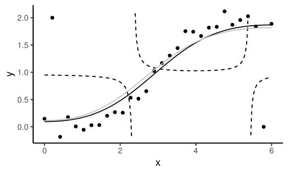
We first consider a dataset generated from a hyperbolic tangent function which has a sigmoidal shape
where and ; see Figure 1. This dataset will be referred to as HT0 for the remainder of this paper. Our objective is to fit the following rational function model
| (9) |
which has a horizontal asymptote at , to the HT0 dataset, subject to a increasing monotonicity constraint in the interval . The necessary conditions for this constraint are
| (10) |
and
| (11) |
where (10) is necessary for the first derivative of to be non-negative, and (11) for to be continuous, in the interval . Although both (10) and (11) are not closed-form expressions, these conditions can be verified easily. For (10), the left hand side of the inequality, which itself is a polynomial, needs to fulfil two conditions: (i) all roots of the polynomial in must have even multiplicities; and (ii) the polynomial must evaluate to a positive number at an arbitrary in . To verify (11), we only need to ensure that the polynomial does not have any roots in .
We use a least squares estimator, which minimises the model’s residual sums of squares
| (12) |
where , to obtain the best fit of (9) to HT0. A rough estimate for generating starting states was obtained from a linear model rearranged from (9)
| (13) |
The pilot estimate for CEPSO was an unconstrained least squares estimate obtained from the Newton-Gauss algorithm implemented in R. The rough estimate was used as the starting value for the Newton-Gauss algorithm.
| Algorithms | Mean | SD | Min | Med | Max | #Conv | Time |
|---|---|---|---|---|---|---|---|
| SMC-SA, reciprocal () | 1.224 | 0.61 | 0.455 | 1.649 | 1.781 | 14 | 326 |
| SMC-SA, reciprocal () | 1.186 | 0.638 | 0.455 | 1.681 | 1.782 | 16 | 687 |
| SMC-SA, logarithm | 1.565 | 0.236 | 0.464 | 1.614 | 1.801 | 0 | 636 |
| multi-start SA | 1.185 | 0.313 | 0.532 | 1.329 | 1.585 | 0 | 293 |
| CEPSO | 0.570 | 0.362 | 0.458 | 0.470 | 1.824 | 4 | 442 |
| Algorithms | Mean | SD | Min | Med | Max | #Conv | Time |
|---|---|---|---|---|---|---|---|
| SMC-SA, reciprocal () | 1.296 | 0.568 | 0.455 | 1.646 | 1.772 | 11 | 375 |
| SMC-SA, reciprocal () | 1.463 | 0.488 | 0.455 | 1.688 | 1.963 | 6 | 374 |
| SMC-SA, logarithm | 1.615 | 0.113 | 1.363 | 1.639 | 1.767 | 0 | 296 |
| multi-start SA | 1.296 | 0.201 | 0.509 | 1.328 | 1.558 | 0 | 309 |
For this example, we tried SMC-SA, multi-start SA and CEPSO with different hyperparameters. The results from SA-based algorithms with a 2-point operator proposal and CEPSO are presented in Table 3. In terms of the best estimate achieved, SMC-SA with a reciprocal schedule attained the lowest loss function value (), followed by CEPSO (). CEPSO generally has a higher chance of converging to the area near compared with SA-based algorithms, as shown in the medians of the loss function values; although, SMC-SA with a reciprocal schedule can produce a more accurate estimate, as demonstrated in the number of chains with a loss function value within 1% of the lowest achieved in this simulation study. The hyperparameter in the reciprocal schedule also did not have a significant impact on the convergence of SMC-SA. However, SMC-SA with the logarithm schedule and multi-start SA are less robust in the sense that the algorithms either did not converge (i.e. high median of or produced inaccurate estimates (i.e. no chain getting close to the best ). The results from SA-based algorithms with a 1-point operator proposal are presented in Table 3, which does not indicate any significant difference in the summary statistics of loss function values between using a 1-point and 2-point operator proposal. Nevertheless, SMC-SA with a reciprocal schedule was more likely to produce accurate estimates when using a 2-point operator proposal, as shown in the higher proportion of chains achieving (14 and 16 out of 40 in Table 2 compared to 11 and 6 out of 40 in Table 3).
| Algorithms | Iterations | |||||
|---|---|---|---|---|---|---|
| 100 | 200 | 400 | 1000 | 2000 | 3000 | |
| SMC-SA, recip. | 1.314 (0) | 1.231 (14) | 1.224 (14) | 1.224 (14) | NA | NA |
| SMC-SA, log. | 1.683 (0) | 1.656 (0) | 1.634 (0) | 1.605 (0) | 1.565 (0) | 1.565 (0) |
| multi-start SA | 1.764 (0) | 1.713 (0) | 1.639 (0) | 1.429 (0) | 1.241 (0) | 1.185 (0) |
| CEPSO | 0.681 (0) | 0.598 (0) | 0.582 (1) | 0.574 (2) | 0.57 (4) | NA |
In Table 4, we have also included the means of loss function values and the number of chains achieving when the algorithm stopped at different iterations. The estimate generally improved slowly as the algorithm iterates, with the exception of SMC-SA with a reciprocal schedule which achieved 14 estimates that were close to in the first 400 iterations and plateaued thereafter. This observation motivates using a reciprocal schedule instead of a logarithm schedule to save computational resources, as we can terminate the SMC-SA well before iterating 1000 times. However, we still iterated 1000 times in this simulation study to ensure that all algorithms consume roughly the same amount of computational resources.
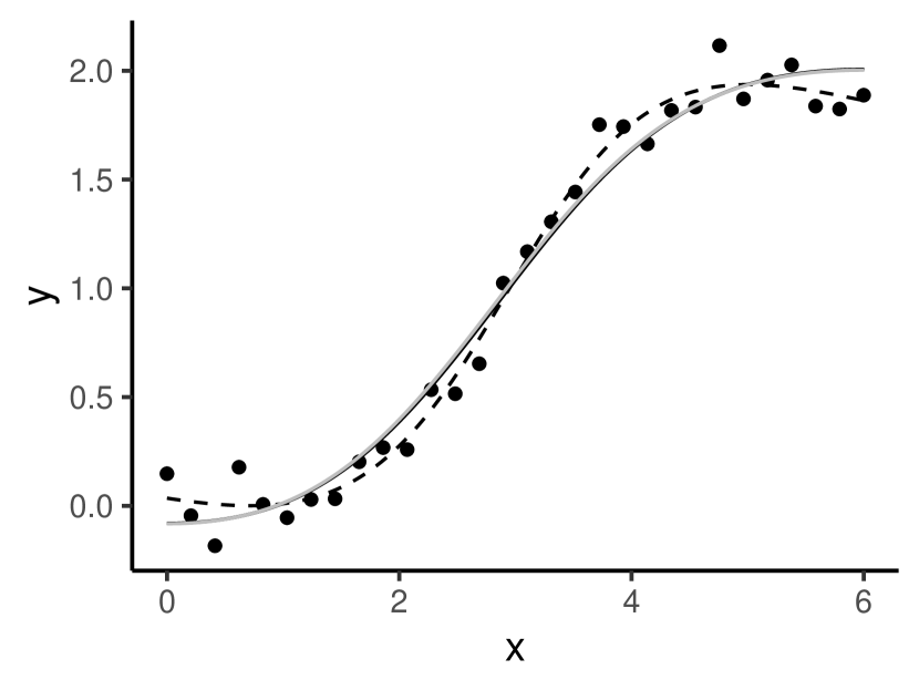
The least squares curves produced by SMC-SA, multi-start SA and CEPSO are illustrated in Figure 1, with the unconstrained least squares curve (black dotted) serving as a reference. Since the results produced by SMC-SA and CEPSO did not differ greatly, their regression curves are overlaying one another, and thus appear to be a single curve. Conversely, there is a noticeable difference between the curves produced from SMC-SA and multi-start SA, as the best estimate attained by the latter was sub-optimal. From these results, we conclude that SMC-SA can produce estimates comparable to that from CEPSO but without the need of a pilot estimate.
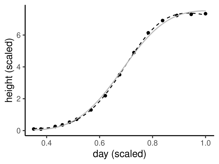
4.1.2 Modelling the growth of Cucumis melo
Rational function models with the same degree of polynomial on the numerator and denominator have a horizontal asymptote, which can be useful when modelling growth curve. For instance, (9) will converge to when . In this example, we demonstrate the practical usage of rational function models by using (9) to model the growth of Cucumis melo seeds that were grown at C. The dataset comprises 15 mean observations of the height of Cucumis melo seeds recorded over 24 days; more details can be found in Pearl et al. (1934). The response (height) and covariate (day) are scaled appropriately for numerical stability.
We constrained the growth curve to be monotonically increasing between the first and last recorded dates as we do not expect the seedlings to reduce in height over time. A least squares estimator was employed to fit (9), and and a pilot estimate were obtained using the same procedure in Section 4.1.1.
| Algorithms | Mean | SD | Min | Med | Max | #Conv | Time |
|---|---|---|---|---|---|---|---|
| SMC-SA, reciprocal () | 0.43 | 0.227 | 0.246 | 0.341 | 1.112 | 10 | 387 |
| SMC-SA, reciprocal () | 0.441 | 0.259 | 0.246 | 0.382 | 1.451 | 7 | 386 |
| SMC-SA, logarithm | 0.639 | 0.626 | 0.247 | 0.373 | 3.029 | 6 | 397 |
| CEPSO | 0.295 | 0.017 | 0.274 | 0.289 | 0.337 | 0 | 407 |
The results from SMC-SA and CEPSO are presented in Table 5. Contrary to the previous example in Section 4.1.1, the cooling schedule in SMC-SA did not affect the convergence noticeably. SMC-SA did manage to produce estimates with a lower loss function value compared with CEPSO, which failed to produced an estimate with a loss function value close to 0.246, which is the lowest loss function value achieved in this simulation. The estimates produced by CEPSO, nonetheless, were more stable compared with that from SMC-SA, in the sense that the estimates are similar to each other. The best regression curves produced by each algorithm are also shown in Figure 2, which does not indicate any visually noticeable difference between the curves produced.

4.2 Constrained robust models
Observed data are sometimes contaminated with outliers, and a different loss function can be used to reduce their influence on the model fit. In this example, we demonstrate that our algorithm is capable of estimating the regression coefficients of (9), subject to both (10) and (11), with an M-estimator (Huber, 1981) which minimises the following loss function
| (14) |
where is carefully chosen to limit the influence of outliers on the overall model fit. The least squares estimator is essentially a special case of (14) where , but this particular choice of greatly inflates the influence of outliers. Here, we employ Tukey’s biweight loss function
where the choice of is arbitrary, but our default value is 1.
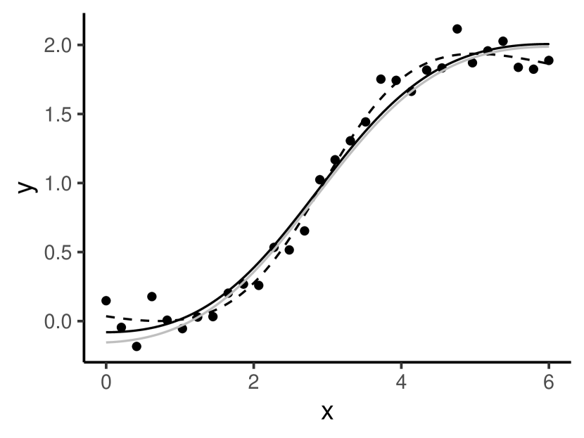
In this example, we used a dataset purposefully contaminated with outliers. This dataset will be referred to as HT1, and was produced by setting the values of and in HT0 to 2 and 0 respectively. We used an unconstrained least squares estimate of (9) fitted on HT0 as the pilot estimate of CEPSO. The estimate was obtained using the Newton-Gauss algorithm starting from , which was obtained following the same procedure described in Section 4.1.1. However, due to the presence of outliers, the estimate obtained from the Newton-Gauss algorithm (the black dotted curve in Figure 3) is a local minimum in the corresponding residual sum of squares function, and thus may not be suitable to be used as the pilot estimate. An unconstrained M-estimate can also be used, but to obtain this will require a different optimisation method.
| Algorithms | Mean | SD | Min | Med | Max | #Conv | Time |
|---|---|---|---|---|---|---|---|
| SMC-SA, reciprocal () | 3.875 | 0.466 | 3.439 | 3.441 | 4.426 | 21 | 365 |
| SMC-SA, reciprocal () | 3.958 | 0.455 | 3.439 | 4.188 | 4.429 | 16 | 680 |
| SMC-SA, logarithm | 4.420 | 0.032 | 4.289 | 4.425 | 4.454 | 0 | 255 |
| CEPSO | 3.573 | 0.149 | 3.489 | 3.567 | 4.452 | 0 | 359 |
In this example, SMC-SA with a reciprocal schedule outperformed CEPSO in terms of the minimum loss function value achieved in 40 runs, as demonstrated in Table 6. There is also a noticeable difference in the regression curves produced by SMC-SA and CEPSO (Figure 3). Since we were using a sub-optimal pilot estimate, we expect that CEPSO would struggle to produce accurate estimates when comparing with SMC-SA. Therefore, in the absence of a satisfactory pilot estimate, we conclude that SMC-SA is preferable.
4.3 Constrained B-spline models
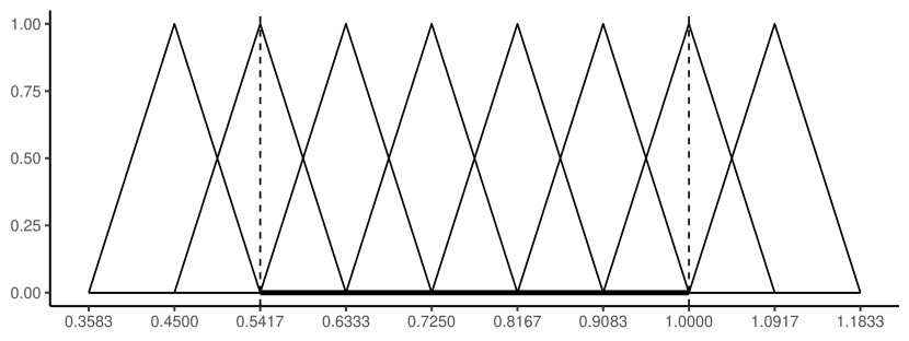
SMC-SA is not restricted to fitting rational function models. In this section, we demonstrate our algorithm by fitting a quadratic B-spline model on a dataset collected from a light detection and ranging (LIDAR) experiment (Sigrist et al., 1994). The data comprises 221 observations of log-ratios of received light from two laser sources (logratio), recorded against the distance travelled before the light is reflected back to its source (range). The log-ratio is expected to decrease as the range increases. For the purpose of this example, both response and covariate were divided by their respective maximum to ensure numerical stability.
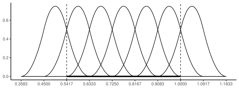
The mathematical formulation of the quadratic B-spline model is given by
| (15) |
where denotes quadratic B-spline basis functions with 10 equidistant knots spanning between the minimum () and maximum () of the covariate; see Figure 4. For the quadratic B-spline model to be monotonically decreasing over the interval , we require the regression coefficients to follow ; further details are given in A. We used a least squares estimator to fit (15) and chose an arbitrary sequence as the rough estimate for generating starting states. The ordinary least squares estimate of (15) was employed as the pilot estimate of CEPSO and admits a close-form expression where , , , and the response vector .
| Algorithms | Mean | SD | Min | Med | Max | #Conv | Time |
|---|---|---|---|---|---|---|---|
| SMC-SA, reciprocal () | 1.530 | 0.001 | 1.530 | 1.530 | 1.530 | 40 | 752 |
| SMC-SA, reciprocal () | 1.530 | 0.001 | 1.530 | 1.530 | 1.530 | 40 | 762 |
| SMC-SA, logarithm | 1.540 | 0.003 | 1.533 | 1.54 | 1.547 | 37 | 2235 |
| CEPSO | 1.530 | 0.001 | 1.530 | 1.530 | 1.530 | 40 | 682 |
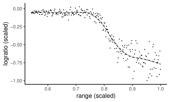
In this example, SMC-SA with a reciprocal schedule produced indistinguishable results to CEPSO, as shown in Table 7, although CEPSO is slightly faster in terms of computation time. More remarkably, all 40 runs of these algorithms converged to the same estimate. This accomplishment is partly attributed to the similarity between the unconstrained and constrained estimates, which can be seen in Figure 5. However, SMC-SA with a logarithm schedule performed slightly worse than the rest in terms of the quality of estimates and took significantly more time to run. This inefficiency is mainly due to the relatively high variance of the proposal of SMC-SA with the logarithm schedule, resulting in the algorithm spending too much effort on exploring rather than refining the estimate. From this result, we can conclude that SMC-SA with a reciprocal schedule is a competitive alternative to CEPSO, with the benefit of not requiring a pilot estimate to operate.
5 Discussion
We introduced a constrained-augmented SMC-SA algorithm which is capable of optimising with a wide variety of constraints, including those that do not have closed-form expressions. Our algorithm only requires an indicator function that verifies the feasibility of an estimate to operate, as opposed to CEPSO which requires an additional pilot estimate which may be difficult to obtain.
Our algorithm was built upon the fact that a Boltzmann distribution will converge to a Dirac measure at the global minimum as the cooling temperature decreases to 0, even when its support is restricted to a subset of a real space. Therefore, we followed the idea of Zhou and Chen (2013) to sample from the sequence of Boltzmann distributions using a SMC sampler. We could similarly use a sampler that incorporates Hamiltonian dynamics, which may explore high-dimensional parameter space more efficiently, or parallel tempering to make our algorithm more robust against local minima. Furthermore, our algorithm can potentially be sped up by augmenting the Boltzmann distribution, as in Liang et al. (2014).
The running time of our algorithm is mainly concentrated on the rejection sampler that generates proposed states from (6). However, the usage of rejection samplers, which is necessary in our algorithm due to the lack of assumptions on the nature of the constraints, is notoriously inefficient for truncating high dimensional distributions, particularly when the probability mass of the untruncated (6) is spreading mainly across the infeasible set. For this reason, it is advisable to start the algorithm with feasible starting values to avoid lengthy computation at the first iteration, although our algorithm works with arbitrary starting values in principle. Moreover, when working with a large set of starting values, the computational time can be further improved by parallelising the SA-move, which is executed independently for each .
Although our algorithm is originally intended to solve shape-constrained regression problems, it can be generalised to solve generic constrained optimisation problems. However, one may expect that a reciprocal schedule, which is suggested for shape-constrained regression, may be less suitable since the cooling schedule is usually dependent on the problem at hand. In such cases, we advise a slight modification to the in (7) before trying an alternative family of cooling schedules when a performance improvement is not immediately attained (Fouskakis and Draper, 2002).
The proposal variance, in particular its decreasing factor, is also crucial to the algorithm convergence. Our motivation of decreasing the variance after each iteration is to maintain a healthy acceptance rate (around 0.2 to 0.5) at the latter stages of the algorithm, when a substantial move from the current states is unlikely to improve the search chain (Zhou and Chen, 2013). During that period, the algorithm should focus on refining the current estimates rather than exploring new regions in the parameter space, and a small proposal variance will facilitate this effort. However, the choice of a (or when using the logarithm schedule) decrement of the proposal in our study may be too aggressive in some situations and prevent the algorithm to explore the parameter space effectively. Hence, the user should adjust the decrement accordingly.
As with all optimisation problems, rescaling of the data is sensible to ensure numerical stability which is reflected in the choice of the scale of our example data presented, which in turn affects the choice of hyperparameters (i.e. cooling schedule and proposal variance).
References
-
Andreani et al. (2013)
Andreani, R., Fukuda, E. H., Silva, P. J. S., 2013. A Gauss–Newton
approach for solving constrained optimization problems using differentiable
exact penalties. Journal of Optimization Theory and Applications 156 (2),
417–449.
URL http://dx.doi.org/10.1007/s10957-012-0114-6 - Bon et al. (2017) Bon, J. J., Murray, K., Turlach, B. A., 2017. Fitting monotone polynomials in mixed effects models. Statistics and Computing, 1–20.
-
Brezger and Steiner (2008)
Brezger, A., Steiner, W. J., 2008. Monotonic regression based on Bayesian
P–splines. Journal of Business & Economic Statistics 26 (1), 90–104.
URL http://dx.doi.org/10.1198/073500107000000223 - De Boor (1978) De Boor, C., 1978. A practical guide to splines. Vol. 27. Springer.
- Del Moral et al. (2006) Del Moral, P., Doucet, A., Jasra, A., 2006. Sequential Monte Carlo samplers. Journal of the Royal Statistical Society: Series B (Statistical Methodology) 68 (3), 411–436.
-
Elphinstone (1983)
Elphinstone, C. D., 1983. A target distribution model for nonparametric density
estimation. Communications in Statistics - Theory and Methods 12 (2),
161–198.
URL http://dx.doi.org/10.1080/03610928308828450 - Fouskakis and Draper (2002) Fouskakis, D., Draper, D., 2002. Stochastic optimization: a review. International Statistical Review 70 (3), 315–349.
- Hastings (1970) Hastings, W. K., 1970. Monte Carlo sampling methods using Markov chains and their applications. Biometrika 57 (1), 97–109.
- Hazelton and Turlach (2011) Hazelton, M. L., Turlach, B. A., 2011. Semiparametric regression with shape-constrained penalized splines. Computational Statistics & Data Analysis 55 (10), 2871–2879.
- Huber (1981) Huber, P. J., 1981. Robust statistics. John Wiley & Sons.
-
Kelly and Rice (1990)
Kelly, C., Rice, J., 1990. Monotone smoothing with application to dose-response
curves and the assessment of synergism. Biometrics 46 (4), 1071–1085.
URL http://www.jstor.org/stable/2532449 -
Kirkpatrick et al. (1983)
Kirkpatrick, S., Gelatt, Jr., C. D., Vecchi, M. P., 1983. Optimization by
simulated annealing. Science 220 (4598), 671–680.
URL http://dx.doi.org/10.1126/science.220.4598.671 -
Leitenstorfer and Tutz (2007)
Leitenstorfer, F., Tutz, G., 2007. Generalized monotonic regression based on
B-splines with an application to air pollution data. Biostatistics 8 (3),
654–673.
URL http://dx.doi.org/10.1093/biostatistics/kxl036 - Liang et al. (2014) Liang, F., Cheng, Y., Lin, G., 2014. Simulated stochastic approximation annealing for global optimization with a square-root cooling schedule. Journal of the American Statistical Association 109 (506), 847–863.
- Locatelli (2000) Locatelli, M., 2000. Simulated annealing algorithms for continuous global optimization: convergence conditions. Journal of Optimization Theory and Applications 104 (1), 121–133.
- Locatelli (2002) Locatelli, M., 2002. Simulated annealing algorithms for continuous global optimization. In: Handbook of global optimization. Springer, pp. 179–229.
- Manderson et al. (2017) Manderson, A. A., Cripps, E., Murray, K., Turlach, B. A., 2017. Monotone polynomials using BUGS and Stan. Australian & New Zealand Journal of Statistics 59 (4), 353–370.
- Marsh (1980) Marsh, H., 1980. Age determination of the dugong (Dugong dugon (Müller)) and its biological implications. International Whaling Commission Reports (Special Issue), 181–201.
-
Matzkin (1991)
Matzkin, R. L., 1991. Semiparametric estimation of monotone and concave utility
functions for polychotomous choice models. Econometrica 59 (5), 1315–1327.
URL http://www.jstor.org/stable/2938369 - Metropolis et al. (1953) Metropolis, N., Rosenbluth, A. W., Rosenbluth, M. N., Teller, A. H., Teller, E., 1953. Equation of state calculations by fast computing machines. The Journal of Chemical Physics 21 (6), 1087–1092.
- Meyer (2003) Meyer, M. C., 2003. An evolutionary algorithm with applications to statistics. Journal of Computational and Graphical Statistics 12 (2), 265–281.
-
Meyer (2012)
Meyer, M. C., 2012. Constrained penalized splines. Canadian Journal of
Statistics 40 (1), 190–206.
URL http://dx.doi.org/10.1002/cjs.10137 - Meyer et al. (2011) Meyer, M. C., Hackstadt, A. J., Hoeting, J. A., 2011. Bayesian estimation and inference for generalised partial linear models using shape-restricted splines. Journal of Nonparametric Statistics 23 (4), 867–884.
-
Murray et al. (2013)
Murray, K., Müller, S., Turlach, B. A., 2013. Revisiting fitting monotone
polynomials to data. Computational Statistics 28 (5), 1989–2005.
URL http://dx.doi.org/10.1007/s00180-012-0390-5 -
Murray et al. (2016)
Murray, K., Müller, S., Turlach, B. A., 2016. Fast and flexible methods for
monotone polynomial fitting. Journal of Statistical Computation and
Simulation 86 (15), 2946–2966.
URL http://dx.doi.org/10.1080/00949655.2016.1139582 -
Newman (1964)
Newman, D. J., 03 1964. Rational approximation to . The Michigan
Mathematical Journal 11 (1), 11–14.
URL http://dx.doi.org/10.1307/mmj/1028999029 - Nocedal and Wright (2006) Nocedal, J., Wright, S. J., 2006. Numerical optimization, 2nd Edition. Springer Series in Operations Research and Financial Engineering. Springer.
-
Nourani and Andresen (1998)
Nourani, Y., Andresen, B., 1998. A comparison of simulated annealing cooling
strategies. Journal of Physics A: Mathematical and General 31 (41), 8373.
URL http://stacks.iop.org/0305-4470/31/i=41/a=011 - Pearl et al. (1934) Pearl, R., Edwards, T. I., Miner, J. R., 1934. The growth of Cucumis melo seedlings at different temperatures. The Journal of General Physiology 17 (5), 687.
-
Piegorsch and Bailer (2005)
Piegorsch, W. W., Bailer, A. J., 2005. Nonlinear Regression. John Wiley &
Sons, Ch. 2, pp. 83–87.
URL http://dx.doi.org/10.1002/0470012234.ch2 -
Pya and Wood (2015)
Pya, N., Wood, S. N., May 2015. Shape constrained additive models. Statistics
and Computing 25 (3), 543–559.
URL https://doi.org/10.1007/s11222-013-9448-7 -
R Core Team (2018)
R Core Team, 2018. R: A Language and Environment for Statistical Computing. R
Foundation for Statistical Computing, Vienna, Austria.
URL https://www.R-project.org/ - Ralston and Rabinowitz (2001) Ralston, A., Rabinowitz, P., 2001. A first course in numerical analysis. Courier Corporation.
-
Ramsay (1998)
Ramsay, J. O., 1998. Estimating smooth monotone functions. Journal of the Royal
Statistical Society: Series B (Statistical Methodology) 60 (2), 365–375.
URL http://dx.doi.org/10.1111/1467-9868.00130 - Reddi et al. (2015) Reddi, S. J., Hefny, A., Downey, C., Dubey, A., Sra, S., 2015. Large-scale randomized-coordinate descent methods with non-separable linear constraints. In: Proceedings of the Thirty-First Conference on Uncertainty in Artificial Intelligence. pp. 762–771.
-
Romeijn and Smith (1994)
Romeijn, H. E., Smith, R. L., Sep 1994. Simulated annealing for constrained
global optimization. Journal of Global Optimization 5 (2), 101–126.
URL https://doi.org/10.1007/BF01100688 - Sigrist et al. (1994) Sigrist, M. W., Winefordner, J. D., Kolthoff, I. M., et al., 1994. Air monitoring by spectroscopic techniques. Vol. 127. John Wiley & Sons.
-
Thornley (1999)
Thornley, J. H. M., 1999. Modelling stem height and diameter growth in plants.
Annals of Botany 84 (2), 195.
URL http://dx.doi.org/10.1006/anbo.1999.0908 - Wolters (2012) Wolters, M. A., 2012. A particle swarm algorithm with broad applicability in shape-constrained estimation. Computational Statistics & Data Analysis 56 (10), 2965–2975.
-
Zhou and Chen (2013)
Zhou, E., Chen, X., 2013. Sequential Monte Carlo simulated annealing.
Journal of Global Optimization 55 (1), 101–124.
URL http://dx.doi.org/10.1007/s10898-011-9838-3
Appendix A Monotone B-spline models
A B-spline model with degree and a set of knots can be written as
where only evaluates in . Suppose that knots are equidistant and separated by a distance , the basis functions can be derived from the following recursive formula (De Boor, 1978)
The corresponding first order derivative of is given by
and consequently, can be deduced
| (16) |
The third equality follows from the fact that we are only interested in evaluating for , and that and evaluate to 0 over that interval. For quadratic B-spline models (), we deduce that necessary conditions for decreasing monotonicity, , can be achieved by ensuring that the coefficients of the linear B-spline basis functions in (16), , are non-positive since B-spline basis functions are non-negative everywhere; otherwise, will evaluate to a positive value at at least one knot ; see Figure 6. Therefore, the necessary condition for a monotonically decreasing quadratic spline is . The condition for increasing monotonicity can also be deduced similarly.