Super-Resolution Blind Channel-and-Signal
Estimation for Massive MIMO with
One-Dimensional Antenna Array

Abstract

In this paper, we study blind channel-and-signal estimation by exploiting the burst-sparse structure of angular-domain propagation channels in massive MIMO systems. The state-of-the-art approach utilizes the structured channel sparsity by sampling the angular-domain channel representation with a uniform angle-sampling grid, a.k.a. virtual channel representation. However, this approach is only applicable to uniform linear arrays and may cause a substantial performance loss due to the mismatch between the virtual representation and the true angle information. To tackle these challenges, we propose a sparse channel representation with a super-resolution sampling grid and a hidden Markovian support. Based on this, we develop a novel approximate inference based blind estimation algorithm to estimate the channel and the user signals simultaneously, with emphasis on the adoption of the expectation-maximization method to learn the angle information. Furthermore, we demonstrate the low-complexity implementation of our algorithm, making use of factor graph and message passing principles to compute the marginal posteriors. Numerical results show that our proposed method significantly reduces the estimation error compared to the state-of-the-art approach under various settings, which verifies the efficiency and robustness of our method.

I Introduction

Multiuser massive multi-input multi-output (MIMO) has attracted intensive research interests since it provides remarkable improvements on system capacity and reliability[MIMO_over1, MIMO_over3, MIMO_over4, MIMO_over5]. As one of the key obstacles to utilizing the high array gain of a massive MIMO system, the acquisition of the channel state information (CSI) becomes challenging due to increased channel dimensions and fast channel variations [MIMO_chanllenge]. Many studies have been conducted to design reliable techniques for channel acquisition. For example, a conventional training-based approach estimates the channel coefficients by using orthogonal pilot sequences [MIMO_pilot3, MIMO_pilot4, MIMO_chanllenge2]. Joint channel and signal estimation can further improve the system performance since the estimated signals can be used as “soft pilots” to enhance the channel estimation accuracy [MIMO_pilot7, MIMO_bayes]. However, the training overhead may become unaffordable in a large-dimension system due to the constrained length of the channel coherence time [MIMO_chanllenge3]. Moreover, training-based methods give rise to the pilot contamination problem, for the reason that the number of available orthogonal pilot sequences cannot exceed the sequence length [MIMO_contamination].

In contrast to training-based methods, another line of research, namely blind or semi-blind channel estimation, aims to estimate the channels without or with less help of the training processes. In [MIMO_blind1, MIMO_EVD, MIMO_Neumann], a particular class of algorithms under this category was proposed to rely on a subspace partition of the received signals, by assuming the asymptotic orthogonality of user channels for extremely large MIMO systems. However, subspace-based methods suffer severe estimation inaccuracy since the number of antennas at the receiver is always limited to be finite in practice. More importantly, these methods require very long coherence duration to generate stable channel estimates, which is usually difficult to realize in fast time-varying scenarios.

Recently, experimental studies have evidenced the burst-sparse structure in the angular domain of the physical channels in massive MIMO systems, thanks to the limited number of scatterers in the propagation environment [Channel_Geometry, Channel_3DmmWave]. Inspired by this, recent studies exploited the sparsity of the massive MIMO channel [MIMO_pilot5, MIMO_pilot6] or the low-rankness of the channel covariance matrix [Channel_formular, MIMO_TSPrecent] in the design of training-based channel estimation schemes. The burst-sparse structure of the channel was modeled using Markovian priors to further improve the channel estimation performance [MIMO_TurboCS, MIMO_LiuAN]. Alternatively, a blind channel estimation method based on channel sparsity was proposed in [MIMO_Amine], where the subspace partition with $\ell_{1}$ regularization was developed to force the sparsity of the channel matrix under the discrete Fourier transform (DFT) angular basis.

To exploit the channel sparsity more efficiently, the authors in [MIMO_zhangjianwen] developed a blind massive MIMO channel-and-signal estimation scheme that simultaneously estimates the channel and detects the transmitted signal from the received signal. It was shown in [MIMO_zhangjianwen] that the channel sparsity leads to a fundamental performance gain on the degrees of freedom of the massive MIMO system. The authors in [MIMO_zhangjianwen] also proposed a modified bilinear generalized approximate message passing (BiG-AMP) algorithm [MP_BIGAMP1], termed projection-based BiG-AMP (Pro-BiG-AMP), to efficiently factorize the sparse channel matrix and the signal matrix.

The existing sparsity-learning based blind channel estimation methods [MIMO_Amine, MIMO_zhangjianwen] assume half-wavelength uniform linear antenna arrays (ULAs). Then, with a uniform sampling grid and a DFT basis, the virtual channel representation model [Channel_virtual_representation, Channel_ExperimentalVR] is employed to characterize the angular-domain sparsity of the massive MIMO channel. However, the DFT-based virtual channel representation is not applicable to ULAs with a non-uniform sampling grid, letting alone antenna arrays with arbitrary geometry. More importantly, the channel estimation accuracy of all DFT-based methods is severely compromised even for ULAs, not only due to the leakage of energy in the DFT basis, but also because the DFT basis is not adaptable to efficiently exploit the burst-sparse structure of the physical channels. To tackle the defects of the existing blind estimation methods, we model the massive MIMO channel using the non-uniform angle-sampling [MIMO_Ding] and the off-grid representation [MIMO_DOA1, OFFGRID_1, OFFGRID_2, OFFGRID_3]. Based on this, we formulate the blind channel estimation problem as an affine matrix factorization (AMF) problem and propose an efficient super-resolution blind channel-and-signal estimation algorithm based on approximate inference and expectation-maximization (EM) principles. The main contributions of this paper are summarized as follows.

• Non-uniform angle-sampling and sparse representation with Markovian support for blind channel-and-signal estimation problem:

  Unlike the existing blind estimation methods that adopt the DFT basis representation, we unfix the angle-of-arrival (AoA) sampling grid and employ an off-grid channel model in massive MIMO. Although the non-DFT sampling basis and the off-grid model have been employed previously in [MIMO_Ding, MIMO_DOA1], this is the first work to adapt the idea to the joint channel-and-signal estimation problem. As such, we formulate the problem as an AMF task with unknown parameters, where the existing off-grid frameworks are not applicable. Following the prior work in [MIMO_TurboCS, MIMO_LiuAN], we employ a set of Markov chains, one for each user, to model the probability space of the channel support. The framework does not impose any restrictions on angle sampling, and hence is able to avoid the energy leakage problem by achieving a resolution much higher than uniform sampling. Moreover, with the Markovian structure, our proposed framework is able to capture the burst-sparse nature of the massive MIMO channel.

• Super-resolution blind channel-and-signal estimation via approximate-inference-based EM:

  We develop a novel blind channel-and-signal estimation method based on EM principles. We show that the exact posterior distributions required by the expectation step (E-step) is difficult to acquire for the bilinear system model with both channel and signal unknown. As such, we propose to utilize approximate inference for the realization of the E-step, hence the name approximate-inference-based EM. Since the proposed solution is designed on top of the off-grid channel representation with the Markovian support, our solution operates with general one-dimensional array geometry and overcomes the angle mismatch problem in the DFT-based methods. Furthermore, under the EM framework, angle-tuning and hyper-parameter learning are employed to learn the AoAs automatically without any prior knowledge of the CSI. We also show that the proposed scheme demonstrates a superior performance to the existing super-resolution algorithm in [MIMO_DOA1] under the joint channel-and-signal estimation framework.

• Marginal posterior calculation via message passing:

  We present a low-complexity implementation of the proposed algorithm. Specifically, as the EM involves the calculation of marginals, we construct an associated factor graph and apply the message passing principles to achieve this purpose. To further reduce the computation complexity, additional approximations are introduced to particular messages based on the general approximate message passing (AMP) framework [MP_AMP1, MP_GAMP]. Finally, we put forth a simplified message passing algorithm and concrete maximization step (M-step) update rules. Additional guidance for convergence acceleration is provided as well.

The remainder of this paper is organized as follows: Section II describes the system model and introduces the off-grid representation. Investigations on the state-of-the-art blind channel estimation algorithm are conducted in this section as well. In Section III, we derive the proposed blind channel-and-signal estimation algorithm and the associated prior-information learning algorithm. In Section IV, we present the marginal posterior calculation scheme based on message passing. Furthermore, Section LABEL:Simulation gives numerical results on the proposed methods. Finally, the paper concludes in Section LABEL:conclusions.

Notation: Throughout, we use $\mathbb{R}$ and $\mathbb{C}$ to denote the real and complex number sets, respectively. We use regular small letters, bold small letters, and bold capital letters to denote scalars, vectors, and matrices, respectively. We use $x_{ij}$ to denote the entry at the $i$-th row and $j$-th column of matrix ${\bf X}$. We use $(\cdot)^{\star}$, $(\cdot)^{T}$, and $(\cdot)^{H}$ to denote the conjugate, transpose, and conjugate transpose, respectively. We use $\mathbb{E}[\cdot]$ to denote the expectation operator, $\lvert\cdot\rvert$ to denote the absolute operator, $\lVert\cdot\rVert_{p}$ to denote the $\ell_{p}$ norm, $\lVert\cdot\rVert_{F}$ to denote the Frobenius norm, $\delta(\cdot)$ to denote the Dirac delta function, and $\propto$ to denote equality up to a constant multiplicative factor. We use $\mathcal{N}(\cdot;\mu,\sigma^{2})$ and $\mathcal{CN}(\cdot;\mu,\sigma^{2})$ to denote the real normal and circularly-symmetric normal distributions with mean $\mu$ and variance $\sigma^{2}$, respectively. Finally, we define $[n]\triangleq\{1,2,3,\cdots,n\}$ for some positive integer $n$.

II System Model

II-A Massive MIMO Channel Model

Consider a multiuser massive MIMO system with $K$ users equipped with a single antenna and one base station (BS) with $N$ antennas, where $N\gg K\gg 1$. We assume that the channel is block-fading. During coherence time $T$, the uplink channel impulse response from the $k$-th user to the BS can be modeled as [Channel_formular]

$${\bf h}_{k}(t)=\sum_{i=1}^{L_{c}(k)}\sum_{j=1}^{L_{p}(k)}\alpha_{k}(i,j){\bf a}\left(\theta_{k}(i,j)\right)\delta\left(t\!-\!\tau_{k}(i,j)\right),\forall t\in[T],$$ (1)

where $L_{c}(k)$ and $L_{p}(k)$ denote the number of scattering clusters and the number of physical paths in each cluster between the $k$-th user and the BS, respectively; $\alpha_{k}(i,j)$ denotes the complex-valued channel coefficient of the $j$-th path in the $i$-th cluster for the $k$-th user; $\theta_{k}(i,j)$ denotes the corresponding azimuth AoA; $\tau_{k}(i,j)$ denotes the corresponding time delay; and ${\bf a}(\theta)$ is the steering vector for receiving a signal, impinging upon the antenna array at angle $\theta$. In general, ${\bf a}(\theta)$ is determined by the geometry of the antenna array at the BS. For instance, if a ULA is deployed at the BS, ${\bf a}(\theta)$ is given by

$${\bf a}(\theta)=\frac{1}{\sqrt{N}}\left[1,e^{-j\frac{2\pi}{\varrho}d\sin(\theta)},\cdots,e^{-j\frac{2\pi}{\varrho}d(N-1)\sin(\theta)}\right]^{T},$$ (2)

where $\varrho$ denotes the carrier wavelength, and $d$ denotes the distance between any two adjacent antennas. As another example, suppose that the BS is equipped with a lens antenna array (LAA), where the lens antennas are placed on the focal arc of the lens with critical antenna spacing. The steering vector ${\bf a}(\theta)$ is given by (3), where $\text{sinc}(\cdot)$ denotes the nominalized “sinc” function, and $D$ denotes the lens length along the azimuth plane [MIMO_LAA].

$${\bf a}(\theta)=\left[\text{sinc}\left(-\frac{N-1}{2}-\frac{D}{\varrho}\sin\theta\right),\text{sinc}\left(-\frac{N-3}{2}-\frac{D}{\varrho}\sin\theta\right),\cdots,\text{sinc}\left(\frac{N-1}{2}-\frac{D}{\varrho}\sin\theta\right)\right]^{T}.$$ (3)

With the channel impulse response given by (1), the received signal at time $t$ can be expressed as

$${\bf y}(t) =\sum_{k=1}^{K}{\bf h}_{k}(t)\ast x_{k}(t)+{\bf n}(t)$$

$$=\sum_{k=1}^{K}\sum_{i=1}^{L_{c}(k)}\sum_{j=1}^{L_{p}(k)}\alpha_{k}(i,\!j){\bf a}\left(\theta_{k}(i,\!j)\right)x_{k}(t\!-\!\tau_{k}(i,\!j))\!+\!{\bf n}(t),$$ (4)

where $\ast$ denotes the linear convolution operation; $x_{k}(t)\in\mathbb{C}$ is the transmitted symbol from the $k$-th user; and ${\bf n}(t)$ is the channel noise vector.

Assume that the delay spread for different paths is negligible compared to the reciprocal of signal bandwidth $W$, i.e., $|\tau_{k}(i,j)\!-\!\tau_{k}(i^{\prime},j^{\prime})|\!\ll\!1/W$ for $\forall(i,j),(i^{\prime}\!,j^{\prime}\!)$. We further simplify (II-A) by approximating different delays with the same value, i.e., $\tau_{k}(i,j)\!\approx\!\tau_{k}$. Therefore, with time synchronization at the receiver side, we can rewrite (II-A) as

$${\bf y}(t)=\sum_{k=1}^{K}\tilde{{\bf h}}_{k}x_{k}(t)+{\bf n}(t),$$ (5)

where the channel coefficient vector of the $k$-th user is defined as

$$\tilde{{\bf h}}_{k}\triangleq\sum_{i=1}^{L_{c}(k)}\sum_{j=1}^{L_{p}(k)}\alpha_{k}(i,j){\bf a}\left(\theta_{k}(i,j)\right).$$ (6)

II-B Off-Grid Representation

Let $\bm{\vartheta}=\{\vartheta_{l}\}^{L}_{l=1}$ be a given grid that consists of $L$ discrete angular points and covers the AoAs ranging from $-90^{\circ}$ to $90^{\circ}$. Denote by $\bm{\theta}\triangleq\{\theta_{k}(i,j)\}_{\forall k,i,j}$ the collection of true AoAs. When $L$ becomes large enough such that $\bm{\theta}\!\subseteq\!\bm{\vartheta}$, (6) can be represented as

$$\tilde{{\bf h}}_{k}=\sum_{l=1}^{L}s_{k,l}{\bf a}(\vartheta_{l})={\bf A}(\bm{\vartheta}){\bf s}_{k},$$ (7)

where ${\bf A}(\bm{\vartheta})\!\triangleq\![{\bf a}(\vartheta_{1}),{\bf a}(\vartheta_{2}),\cdots,{\bf a}(\vartheta_{L})]\!\in\!\mathbb{C}^{N\times L}$ is the angular array response for given $\bm{\vartheta}$, and ${\bf s}_{k}\triangleq[s_{k,1},s_{k,2},\cdots,s_{k,L}]^{T}\in\mathbb{C}^{L\times 1}$ contains the corresponding channel coefficients in the angular domain. More specifically, we have

$${s_{k,l}\!=\!}\begin{cases}\alpha_{k}(i,j),&\text{if }\vartheta_{l}\!=\!\theta_{k}(i,j)\text{ for some }\theta_{k}(i,j)\!\in\!\bm{\theta},\\ 0,&\text{otherwise.}\end{cases}$$ (8)

In fact, $\bm{\vartheta}$ can be viewed as a set of angular resolution bins located at the BS. In practice, since the scattering clusters usually have certain distances from the BS, the subpath associated with a particular scattering cluster will only have a small range of angular spread [Channel_Geometry]. Moreover, since the number of scatterers is usually very small [Channel_Geometry, Channel_3DmmWave], only a small portion of resolution bins will be occupied [Channel_virtual_representation, Channel_ExperimentalVR]. Therefore, if the selected grid $\bm{\vartheta}$ covers the true directions $\bm{\theta}$ well, ${\bf s}_{k}$ will be sparse and the non-zero elements of ${\bf s}_{k}$ will concentrate in a narrow range around a few positions [MIMO_DOA1]. We refer to this phenomenon as the burst-sparse structure of channel coefficient vectors in the angular domain. However, the direction mismatch generally exists between $\bm{\theta}$ and $\bm{\vartheta}$, since the true AoAs are difficult to acquire in practice. To address this problem, we propose an automatic angle tuning scheme for $\bm{\vartheta}$ in Section III.

For each coherence duration $T$, we denote the transmission signals for the $k$-th user by ${\bf x}_{k}\!=\!\left[x_{k}(1),x_{k}(2),\cdots,x_{k}(T)\right]^{T}$, and denote the collection of all transmission signals by ${\bf X}\!=\!\left[{\bf x}_{1},{\bf x}_{2},\cdots,{\bf x}_{K}\right]^{T}\!\in\!\mathbb{C}^{K\times T}$. Then, we represent the received signal by

$${\bf Y}={\bf A}(\bm{\vartheta}){\bf S}{\bf X}+{\bf N},$$ (9)

where ${\bf Y}\!=\![{\bf y}(1),{\bf y}(2),\cdots,{\bf y}(T)]\!\in\!\mathbb{C}^{N\times T}$ denotes the collection of the received signals; ${\bf S}\!=\![{\bf s}_{1},{\bf s}_{2},\cdots,{\bf s}_{K}]\!\in\!\mathbb{C}^{L\times K}$ is the corresponding channel coefficient matrix in the angular domain; and ${\bf N}\in\mathbb{C}^{N\times T}$ denotes an additive white Gaussian noise (AWGN) matrix with the entries i.i.d. drawn from $\mathcal{CN}(\cdot;0,\sigma^{2})$.

Let $P_{k}$ denote the average transmission power for the $k$-th user in duration $T$. Denote by $P\triangleq\sum_{k=1}^{K}P_{k}$ the total average transmission power. For a transmission sequence ${\bf x}_{k}$, by the definition of $P_{k}$ we have

$$\frac{1}{T}\mathbb{E}[{\bf x}_{k}^{H}{\bf x}_{k}]=P_{k},\text{ for }\forall k\in[K].$$ (10)

Without loss of generality, we assume $P=K$ in the sequel. Additionally, we assume $P_{k}=1$ for $\forall k$.

II-C Channel Representation with DFT Basis

Here, we discuss a state-of-the-art framework for blindly estimating user signals from (9) and specify its potential limitations. Suppose that the BS is equipped with a ULA. A framework called virtual channel representation [Channel_virtual_representation, Channel_ExperimentalVR] was proposed to resolve the channel by a fixed sampling grid $\bm{\vartheta}^{0}$ with length $L=N$. Specifically, $\bm{\vartheta}^{0}$ satisfies

$$\frac{d}{\varrho}\sin(\vartheta^{0}_{n})=\frac{n-1}{N},\forall n\in[N].$$ (11)

Substituting (11) into (2), we see that ${\bf A}(\bm{\vartheta}^{0})$ is the normalized DFT matrix denoted by ${\bf F}$. Thus, we obtain

$${\tilde{{\bf Y}}}={\bf F}^{H}{\bf Y}={\tilde{{\bf S}}}{\bf X}+{\tilde{{\bf N}}},$$ (12)

where ${\tilde{{\bf S}}}={\bf F}^{H}{\bf A}(\bm{\theta}){\bf S}\in\mathbb{C}^{N\times K}$ is the channel representation under the DFT basis, and the entries of ${\tilde{{\bf N}}}$ are i.i.d. drawn from $\mathcal{CN}(\cdot;0,\sigma^{2})$.

Existing blind estimation methods [MIMO_zhangjianwen, MIMO_Amine] aim to recover both the channel ${\tilde{{\bf S}}}$ and the signal ${\bf X}$ from the observation of ${\tilde{{\bf Y}}}$ in (12) by exploiting the sparsity of ${\tilde{{\bf S}}}$. However, this framework suffers from at least three defects:

• The DFT matrix can only approximate the array response of a ULA. For a general antenna geometry, we may not be able to project the received signal matrix to the angular domain by a simple unitary transformation.

• Since the number of antennas at the BS $N$ is physically constrained to be finite, the DFT-based methods always have performance loss due to the unavoidable AoA mismatch between $\bm{\vartheta}^{0}$ and $\bm{\theta}$, a.k.a. the energy leakage phenomenon. More importantly, due to the energy leakage, the channel matrix ${\tilde{{\bf S}}}$ is not exactly sparse. This may seriously compromise the performance of the channel estimation and signal estimation methods based on the channel sparsity.

• As mentioned in Section II-B, the true AoAs tend to concentrate in a few groups due to a limited number of scattering clusters. The DFT-based methods fail to exploit this burst-sparse structure since they sample the AoA range uniformly.

To address the above defects, we develop a novel framework to blindly estimate the channel matrix and the user signals. We tackle the problem directly based on the signal model (9), without resorting to the DFT-based simplification in (12). We assume general one-dimensional array geometry at the BS and use a general form of the steering vector ${\bf a}(\theta)$ in the derivation. Extensions of the following framework for higher-dimensional antenna arrays are possible but is not the focus of this paper.

III Super-Resolution Blind Channel-and-Signal Estimation

In this section, we develop a framework to infer ${\bf S}$ and ${\bf X}$ given ${\bf Y}$ in (9), a.k.a. the AMF problem. Besides, we discuss how to estimate the latent parameters and tune the grid $\bm{\vartheta}$ in the proposed algorithm.

III-A Probabilistic Model

Define ${\bf W}\triangleq{\bf S}{\bf X}\!\in\!\mathbb{C}^{L\times T}$ and ${\bf Z}\triangleq{\bf A}(\bm{\vartheta}){\bf W}\!\in\!\mathbb{C}^{N\times T}$. Under the assumption of AWGN, we have

$$p({\bf Y}|{\bf Z})=\prod_{n=1}^{N}\prod_{t=1}^{T}\mathcal{CN}\left(y_{nt};z_{nt},\sigma^{2}\right).$$ (13)

For simplicity, we assume that all signals are generated independently, i.e.,

$$p({\bf X})=\prod_{k=1}^{K}\prod_{t=1}^{T}p_{x_{kt}}\left(x_{kt}\right),$$ (14)

where $p_{x_{kt}}(x_{kt})$ is determined by the signal generation model at the transmitter side. Moreover, the hidden sparsity of ${\bf S}$ motivates us to model the prior distribution of ${\bf S}$ as

$$p({\bf S}|{\bf C})=\prod_{l=1}^{L}\prod_{k=1}^{K}\delta\left(c_{lk}\right)\delta\left(s_{lk}\right)+\delta\left(c_{lk}\!-\!1\right)\mathcal{CN}(s_{lk};0,\varphi_{k}),$$ (15)

where the binary state variable $c_{lk}\in\{0,1\}$ for $\forall l,k$ is introduced to indicate whether the corresponding entry of ${\bf S}$ is $0$ or not. In other words, ${\bf C}\in\{0,1\}^{L\times K}$ is the support for ${\bf S}$. Following [MIMO_EVD], we assign a Gaussian prior distribution with zero mean and distinct variance to each non-zero entry of ${\bf S}$. Note that here we set $\varphi_{k}$ to be independent of the antenna grid index $l$.

An intuitive approach to model the support matrix ${\bf C}$ is to assign an i.i.d. Bernoulli distribution to its entries, i.e.,

$$p\left(c_{lk}=1\right)=\lambda,\forall l,k,$$ (16)

where $\lambda$ is the Bernoulli parameter. However, as discussed in Section II-B, the non-zero elements of ${\bf C}$ can be grouped into a small number of clusters. We characterize such a clustered structure of ${\bf C}$ using a set of Markov chains as

$$p({\bf C})=\prod_{k=1}^{K}\left(p(c_{1k})\prod_{l=2}^{L}p\left(c_{lk}|c_{l-1,k}\right)\right).$$ (17)

The transition probabilities are defined as $p\left(c_{lk}=0|c_{l-1,k}=1\right)\triangleq p_{01}$ and $p\left(c_{lk}=1|c_{l-1,k}=0\right)=p_{01}\lambda/(1-\lambda)\triangleq p_{10}$. These definitions ensure that each Markov chain is consistent with the marginal distribution (16) with $p\left(c_{1k}=1\right)$ set to $\lambda$. Therefore, by marginalizing $c_{lk}$, we obtain

$$p_{s_{lk}}(s_{lk})=(1-\lambda)\delta(s_{lk})+\lambda\mathcal{CN}\left(s_{lk};0,\varphi_{k}\right).$$ (18)

III-B Inference by Expectation-Maximization

Given the prior distributions, the maximum a posterior (MAP) estimator (${\hat{\bf X}}$, ${\hat{\bf S}}$) is given by

$$({\hat{\bf X}},{\hat{\bf S}})=\operatorname*{argmax}_{{\bf X},{\bf S}}\int_{{\bf C}}p({\bf X},{\bf S},{\bf C}|{\bf Y}).$$ (19)

The computation of (19) requires the knowledge of prior distributions (13)–(18). While $p_{x_{kt}}(x_{kt})$ can be obtained from the transmitters, parameters $\sigma^{2}$, $\bm{\varphi}$, $p_{01}$, and $\lambda$ in $p({\bf Y}|{\bf Z})$, $p({\bf S}|{\bf C})$, and $p({\bf C})$ are usually difficult to extract before the estimation procedure. Besides, as mentioned in Section II-B, the AoA directions in $\bm{\vartheta}$ may be difficult to acquire in general. Following the EM principle [DL_Goodfellow], we infer the posterior distribution $p({\bf X},{\bf S},{\bf C}|{\bf Y})$ with unknown parameters $\Psi\triangleq\{\sigma^{2},\lambda,p_{01},\bm{\varphi},\bm{\vartheta}\}$ by maximizing the corresponding evidence lower bound (ELBO) $\mathcal{L}({\bf Y},\Psi,q)$, i.e.

$$p({\bf X},{\bf S},{\bf C}|{\bf Y})=\operatorname*{argmax}_{q}\underbrace{\mathbb{E}_{q}\left[\ln p({\bf Y},{\bf X},{\bf S},{\bf C};\Psi)\right]+H(q)}_{\mathcal{L}({\bf Y},\Psi,q)},$$ (20)

where the expectation is w.r.t. an arbitrary probability distribution $q$ over ${\bf X}$, ${\bf S}$ and ${\bf C}$, and $H(\cdot)$ is the entropy function.

The EM algorithm maximizes $\mathcal{L}$ with respect to $q$ and $\Psi$ in an alternating fashion. The detailed steps are as follows.

• E-step: Denote the initial guess of the parameters as $\Psi^{(0)}$. At the $j$-th iteration, set $q^{(j)}({\bf X},{\bf S},{\bf C}|{\bf Y})=p({\bf X},{\bf S},{\bf C}|{\bf Y};\Psi^{(j)})$. In other words, $q$ is defined as the posterior in terms of the current value of $\Psi$.

• M-step: Update $\Psi^{(j+1)}$ by

  $$\Psi^{(j+1)} =\operatorname*{argmax}_{\Psi}\mathcal{L}({\bf Y},\Psi,q^{(j)})$$

  $$=\operatorname*{argmax}_{\Psi}\mathbb{E}_{q^{(j)}}\left[\ln p({\bf Y},{\bf X},{\bf S},{\bf C};\Psi)\right].$$ (21)

In the sequel, we discuss our design to realize the EM algorithm based on the idea of approximate inference.

III-C Approximate-Inference-Based EM Algorithm

The posterior $q^{(j)}$ in each iteration is generally intractable even for given $\Psi^{(j)}$. We realize the E-step by restricting a particular family of distribution $q$, a.k.a. approximate inference[DL_Goodfellow]. Here, we set $q$ as a factorizable distribution. In other words, aforementioned $q^{(j)}$ is approximated by the product of the marginal distributions as

$$q^{(j)} ({\bf X},{\bf S},{\bf C}|{\bf Y})$$

$$=\prod_{k=1}^{K}\prod_{t=1}^{T}p(x_{kt}|{\bf Y};\Psi^{(j)})\prod_{l=1}^{L}\prod_{k=1}^{K}p(s_{lk},\!c_{lk}|{\bf Y};\Psi^{(j)}).$$ (22)

Remark 1.

The proposed approximation in (III-C) seems similar to, but is different from the idea of variational inference. Specifically, variational inference aims to find the factorizable distribution $\tilde{q}({\bf X},{\bf S},{\bf C})\triangleq\prod_{k=1}^{K}\prod_{t=1}^{T}q_{kt}(x_{kt})\prod_{l=1}^{L}\prod_{k=1}^{K}q_{lk}(s_{lk},c_{lk})$, such that the Kullback-Leibler divergence w.r.t. the target distribution $\text{KL}(\tilde{q}({\bf X},{\bf S},{\bf C})\!\!\parallel\!\!p({\bf X},{\bf S},{\bf C}|{\bf Y};\Psi^{(j)}))$ is minimized. However, here we approximate the true posterior as the product of marginal distributions. It is shown in [PRML] that the proposed approximation corresponds to the minimizer of the inverse Kullback-Leibler divergence $\text{KL}(p({\bf X},{\bf S},{\bf C}|{\bf Y};\Psi^{(j)})\!\parallel\!q^{(j)}({\bf X},{\bf S},{\bf C}|{\bf Y}))$.

We adopt the incremental variant scheme [NN_EM2] and perform coordinate-wise maximization to update the elements in $\Psi$ sequentially. Specifically, we have the following update rules for the M-step:

$$(\sigma^{2})^{(j+1)}\!=\! \operatorname*{argmax}_{\sigma^{2}}\mathbb{E}\left[\ln p({\bf Y},\!{\bf X},\!{\bf S},\!{\bf C};\sigma^{2}\!,\!\bm{\vartheta}^{(j)}\!,\!\bm{\varphi}^{(j)},p_{01}^{(j)}\!,\!\lambda^{(j)}\!)\right]\!;$$ (23a)

$$\vartheta_{l}^{(j+1)}\!=\! \operatorname*{argmax}_{\vartheta_{l}}\mathbb{E}\Big{[}\ln p({\bf Y},\!{\bf X},\!{\bf S},\!{\bf C};(\sigma^{2})^{(j\!+\!1)}\!,\!\vartheta_{1}^{(j\!+\!1)}\!,\cdots,$$

$$\vartheta_{l\!-\!1}^{(j\!+\!1)},\vartheta_{l},\vartheta_{l\!+\!1}^{(j)},\cdots,\vartheta_{L}^{(j)},\bm{\varphi}^{(j)},p_{01}^{(j)},\lambda^{(j)})\Big{]},\forall l;$$ (23b)

$$\varphi_{k}^{(j+1)}\!=\! \operatorname*{argmax}_{\varphi_{k}}\mathbb{E}\Big{[}\ln p({\bf Y},\!{\bf X},\!{\bf S},\!{\bf C};\sigma^{(j\!+\!1)},\bm{\vartheta}^{(j\!+\!1)},\varphi_{1}^{(j\!+\!1)},$$

$$\cdots,\varphi_{k\!-\!1}^{(j\!+\!1)},\varphi_{k},\varphi_{k\!+\!1}^{(j)},\cdots,\varphi_{K}^{(j)},p_{01}^{(j)},\lambda^{(j)})\Big{]},\forall k;$$ (23c)

$$p_{01}^{(j+1)}\!=\! \operatorname*{argmax}_{p_{01}}\mathbb{E}\Big{[}\ln p({\bf Y},\!{\bf X},\!{\bf S},\!{\bf C};(\sigma^{2})^{(j\!+\!1)},\bm{\vartheta}^{(j\!+\!1)},$$

$$\bm{\varphi}^{(j\!+\!1)},p_{01},\lambda^{(j)})\Big{]};$$ (23d)

$$\lambda^{(j+1)}= \operatorname*{argmax}_{\lambda}\mathbb{E}\Big{[}\ln p({\bf Y},\!{\bf X},\!{\bf S},\!{\bf C};(\sigma^{2})^{(j\!+\!1)},\bm{\vartheta}^{(j\!+\!1)},$$

$$\bm{\varphi}^{(j\!+\!1)},p_{01}^{(j\!+\!1)},\lambda)\Big{]},$$ (23e)

where the expectations are w.r.t. $q^{(j)}$ defined in (III-C). Note that once we have the exact form of $q^{(j)}$, (23a)–(23e) can be solved efficiently by fixed-point equations. For example, we can solve (23a)–(23e) by forcing the derivative of the objective to zero with respect to the corresponding variable.

The performance of coordinate ascent algorithms may be compromised when the optimized coordinates are correlated. As seen from the probabilistic model in Section III-A, $\bm{\varphi}$, $\lambda$, and $p_{01}$ are tightly coupled. To avoid an oscillation in the iterative process, we update $\bm{\varphi}$, $\lambda$, and $p_{01}$ with multiple times in each iteration to improve the convergence of the overall algorithm.

IV Computation of Marginals and Other Implementation Details

There exist a number of techniques to calculate or approximate the marginal posteriors required in (III-C), such as calculus of variants, sparse Bayesian learning, and message passing. Here, we propose to compute the marginal posteriors in (III-C) by message passing, which is used to execute the M-step in (23a)–(23e).

IV-A Computation of Marginal Posteriors

From the model introduced in Section III-A, we obtain

$$p({\bf Y}, {\bf X},{\bf S},{\bf C})\propto p({\bf Y}|{\bf Z})p({\bf X})p({\bf S}|{\bf C})p({\bf C})\delta({\bf Z}-{\bf A}(\bm{\vartheta}){\bf S}{\bf X})$$

$$\propto \left(\prod_{n=1}^{N}\prod_{t=1}^{T}p(y_{nt}|z_{nt})\delta\!\left(\!z_{nt}\!-\!\sum_{l=1}^{L}\sum_{k=1}^{K}A_{nl}s_{lk}x_{kt}\right)\right)$$

$$\left(\prod_{k=1}^{K}\prod_{t=1}^{T}p_{x_{kt}}(x_{kt})\right)\left(\prod_{l=1}^{L}\prod_{k=1}^{K}p(s_{lk}|c_{lk})p(c_{lk})\right).$$ (24)

The factor graph representation of (24) is depicted in Fig. 1. The factorized pdfs, represented by factor nodes, are connected with their associated arguments, represented by variable nodes. We divide the whole factor graph into two sub-regions to distinguish the AMF structure for (9) and the Markov chain (MC) structure for (17). We summarize the notations of the factors in Table I.

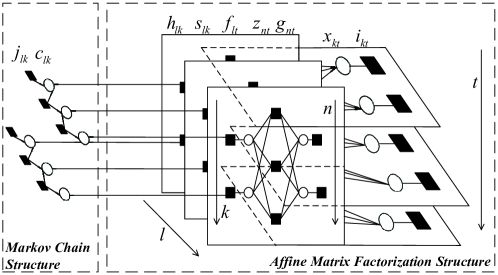
Figure 1: An example of the factor graph representation for $T=L=3$ and $N=K=2$, where empty circles and filled squares represent variable nodes and factor nodes, respectively.

The message passing algorithm on the factor graph in Fig. 1 is described as follows. Denote by $\Delta^{i}_{a\to b}(\cdot)$ the message from node $a$ to $b$ in iteration $i$, and by $\Delta_{c}^{i}(\cdot)$ the marginal posterior computed at variable node $c$ in iteration $i$. Applying the sum-product rules, we obtain the following messages and marginal posteriors.

IV-A1 Messages within the AMF structure

For $\forall n,t,l,k,$

$$\Delta_{z_{nt}\to f_{lt}}^{i}(w_{lt})\propto \int_{\{w_{l^{\prime}\!t}\}_{l^{\prime}\!\neq l}}\!p_{y_{nt}|z_{nt}}(y_{nt}|\sum_{l=1}^{L}A_{nl}w_{lt})$$

$$\prod_{l^{\prime}\!\neq l}\Delta^{i}_{f_{l^{\prime}\!t}\to z_{nt}}(w_{l^{\prime}\!t});$$ (25)

$$\Delta_{f_{lt}\to z_{nt}}^{i\!+\!1}(w_{lt})\propto p^{i}_{w_{lt}}(w_{lt})\prod_{n^{\prime}\!\neq n}\Delta^{i}_{z_{n^{\prime}\!t}\to f_{lt}}(w_{lt});$$ (26)

$$\Delta_{f_{lt}\to x_{kt}}^{i}(x_{kt})\propto \int_{\{s_{lk}\}_{\forall k},\{x_{k^{\prime}\!t}\}_{k^{\prime}\!\neq k}}\prod_{k=1}^{K}\Delta_{s_{lk}\to f_{lt}}^{i}(s_{lk})$$

$$\prod_{k^{\prime}\!\neq k}\Delta_{x_{k^{\prime}\!t}\to f_{lt}}^{i}(x_{k^{\prime}\!t})\prod_{n=1}^{N}\Delta_{z_{nt}\to f_{lt}}^{i}(w_{lt});$$ (27)

$$\Delta_{x_{kt}\to f_{lt}}^{i\!+\!1}(x_{kt})\propto p_{x_{kt}}(x_{kt})\prod_{l^{\prime}\!\neq l}\Delta_{f_{l^{\prime}\!t}\to x_{kt}}^{i}(x_{kt});$$ (28)

$$\Delta_{f_{lt}\to s_{lk}}^{i}(s_{lk})\propto \int_{\{x_{kt}\}_{\forall k},\{s_{lk^{\prime}}\!\}_{k^{\prime}\!\neq k}}\prod_{k=1}^{K}\Delta_{x_{kt}\to f_{lt}}^{i}(x_{kt})$$

$$\prod_{k^{\prime}\!\neq k}\Delta_{s_{lk^{\prime}}\!\to f_{lt}}^{i}(s_{lk^{\prime}})\prod_{n=1}^{N}\Delta_{z_{nt}\to f_{lt}}^{i}(w_{lt});$$ (29)

$$\Delta_{s_{lk}\to f_{lt}}^{i\!+\!1}(s_{lk})\propto \Delta_{h_{lk}\to s_{lk}}^{i}(s_{lk})\prod_{t^{\prime}\!\neq t}\Delta_{f_{lt^{\prime}}\to s_{lk}}^{i}(s_{lk}),$$ (30)

where $p^{i}_{w_{lt}}(w_{lt})$ in (26) is defined to be

$$p^{i}_{w_{lt}}(w_{lt})\propto \int_{\{s_{lk},x_{kt}\}_{\forall k}}\!\left(\prod_{k=1}^{K}\Delta^{i}_{x_{kt}\to f_{lt}}(x_{kt})\Delta^{i}_{s_{lk}\to f_{lt}}(s_{lk})\right)$$

$$\delta\left(w_{lt}\!-\!\sum_{k=1}^{K}s_{lk}x_{kt}\right).$$ (31)

Table I: Notation for the factor nodes

Factor	Distribution	Exact Form
$f_{lt}$	$p(w_{lt}|s_{lk},x_{kt},\!\forall k)$	$\delta(w_{lt}-\sum_{k}s_{lk}x_{kt})$
$g_{nt}$	$p(y_{nt}|z_{nt})$	$\mathcal{CN}(y_{nt};z_{nt},\sigma^{2})$
$h_{lk}$	$p(s_{lk}|c_{lk})$	$\delta\left(c_{lk}\right)\delta\left(s_{lk}\right)\!+$
		$\delta\left(c_{lk}\!-\!1\right)\mathcal{CN}(s_{lk};0,\varphi_{k})$
$i_{kt}$	$p_{x_{kt}}\left(x_{kt}\right)$	$p_{x_{kt}}\left(x_{kt}\right)$
$j_{lk}$	$p\left(c_{lk}|c_{l\!-\!1,k}\right)$	$\begin{cases}(1\!-\!p_{10})^{1\!-\!c_{lk}}p_{10}^{c_{lk}},c_{l-1,k}\!=\!0\\ p_{01}^{1\!-\!c_{lk}}(1\!-\!p_{01})^{c_{lk}},c_{l-1,k}\!=\!1\end{cases}$

IV-A2 Messages within the MC structure

For $\forall l,k,$ for $l=1,\cdots,L-1$,

$$\Delta_{j_{l\!+\!1,k}\to c_{l\!+\!1,k}}^{i}(c_{l\!+\!1,k})$$

$$\propto\!\sum_{c_{lk}\in\{0,1\}}p\left(c_{l\!+\!1,k}|c_{lk}\right)\Delta_{j_{lk}\!\to\!c_{lk}}^{i}(c_{lk})\Delta_{h_{lk}\!\to\!c_{lk}}^{i}(c_{lk}),$$ (32)

and $\Delta_{j_{1k}\!\to\!c_{1k}}^{i}(c_{1k})$ is set to $(1\!-\!\lambda)\delta(c_{1k})\!+\!\lambda\delta(c_{1k}\!-\!1)$.

For $l=L,L-1,\cdots,2$,

$$\Delta_{j_{lk}\to c_{l\!-\!1,k}}^{i}(c_{l\!-\!1,k})$$

$$\propto\!\sum_{c_{lk}\in\{0,1\}}p\left(c_{lk}|c_{l\!-\!1,k}\right)\Delta_{j_{l\!+\!1,k}\!\to\!c_{lk}}^{i}(c_{lk})\Delta_{h_{lk}\!\to\!c_{lk}}^{i}(c_{lk}),$$ (33)

and $\Delta_{j_{L\!+\!1,k}\!\to\!c_{Lk}}^{i}(c_{Lk})$ is set to $\frac{1}{2}\delta(c_{Lk})\!+\!\frac{1}{2}\delta(c_{Lk}\!-\!1)$.

Table II: Notation of mean and variance for various messages and posteriors

Message/Posterior	Mean	Variance
$\Delta_{f_{lt}\to z_{nt}}^{i}(w_{lt})$	${\hat{w}}_{lt,n}(i)$	$v^{w}_{lt,n}(i)$
$\Delta_{x_{kt}\to f_{lt}}^{i}(x_{kt})$	${\hat{x}}_{kt,l}(i)$	$v^{x}_{kt,l}(i)$
$\Delta_{s_{lk}\to f_{lt}}^{i}(s_{lk})$	${\hat{s}}_{lk,t}(i)$	$v^{s}_{lk,t}(i)$
$\Delta_{x_{kt}}^{i}(x_{kt})$	${\hat{x}}_{kt}(i)$	$v^{x}_{kt}(i)$
$\Delta_{s_{lk}}^{i}(s_{lk})$	${\hat{s}}_{lk}(i)$	$v^{s}_{lk}(i)$

Table III: Messages and posteriors after approximations

Message/Posterior	Functional Form
$\Delta_{h_{lk}\to c_{lk}}^{i}(c_{lk})$	$\pi^{\text{out}}_{lk}(i)$
$\Delta_{c_{lk}\to h_{lk}}^{i}(c_{lk})$	$\pi^{\text{in}}_{lk}(i)$
$\Delta_{j_{lk}\to c_{lk}}^{i}(c_{lk})$	$\lambda^{\text{fwd}}_{lk}(i)$
$\Delta_{j_{l+1,k}\to c_{lk}}^{i}(c_{lk})$	$\lambda^{\text{bwd}}_{lk}(i)$
$\Delta_{c_{lk}}^{i}(c_{lk})$	$\omega_{lk}(i)$
$\Delta_{s_{lk}\to h_{lk}}^{i}(s_{lk})$	$\mathcal{CN}(s_{lk};{\hat{q}}_{lk}(i),v^{q}_{lk}(i))$
$\Delta_{h_{lk}\to s_{lk}}^{i}(s_{lk})$	$\pi^{\text{in}}_{lk}(i)\mathcal{CN}(s_{lk};0,\varphi_{k})\!+\!$
	$(1\!-\!\pi^{\text{in}}_{lk}(i))\delta(s_{lk})$
$\Delta_{f_{lt}\to z_{nt}}^{i}(w_{lt})$	$\mathcal{CN}(w_{lt};{\hat{w}}_{lt,n}(i),v^{w}_{lt,n}(i))$
$\Delta_{x_{kt}\to f_{lt}}^{i}(x_{kt})$	$\frac{1}{Z}\mathcal{CN}(x_{kt};{\hat{r}}_{kt,l}(i),\!v^{r}_{kt,l}(i))p_{x_{kt}}\!\left(x_{kt}\right)$
$\Delta_{s_{lk}\to f_{lt}}^{i}(s_{lk})$	$\frac{1}{Z}\mathcal{CN}(s_{lk};{\hat{q}}_{lk,t}(i),\!v^{q}_{lk,t}(i))\Delta_{h_{lk}\!\to\!s_{lk}}^{i}\!(s_{lk})$
$\Delta_{x_{kt}}^{i}(x_{kt})$	$\frac{1}{Z}\mathcal{CN}(x_{kt};{\hat{r}}_{kt}(i),\!v^{r}_{kt}(i))p_{x_{kt}}\!\left(x_{kt}\right)$
$\Delta_{s_{lk}}^{i}(s_{lk})$	$\frac{1}{Z}\mathcal{CN}(s_{lk};{\hat{q}}_{lk}(i),\!v^{q}_{lk}(i))\Delta_{h_{lk}\!\to\!s_{lk}}^{i}\!(s_{lk})$

IV-A3 Messages exchanged between the MC structure and the AMF structure

For $\forall l,k,$

$$\Delta_{c_{lk}\to h_{lk}}^{i}(c_{lk})\propto \Delta_{j_{lk}\to c_{lk}}^{i}(c_{lk})\Delta_{j_{l\!+\!1,k}\to c_{lk}}^{i}(c_{lk});$$ (34)

$$\Delta_{h_{lk}\to c_{lk}}^{i\!+\!1}(c_{lk})\propto \int_{s_{lk}}p(s_{lk}|c_{lk})\prod_{t=1}^{T}\Delta_{f_{lt}\to s_{lk}}^{i}(s_{lk}).$$ (35)

IV-A4 Marginal functions at variable nodes

For $\forall l,k,t,$

$$\Delta_{x_{kt}}^{i\!+\!1}(x_{kt})\propto p_{x_{kt}}(x_{kt})\prod_{l=1}^{L}\Delta_{f_{lt}\to x_{kt}}^{i}(x_{kt});$$ (36)

$$\Delta_{s_{lk}}^{i\!+\!1}(s_{lk})\propto \Delta_{h_{lk}\to s_{lk}}^{i}(s_{lk})\prod_{t=1}^{T}\Delta_{f_{lt}\to s_{lk}}^{i}(s_{lk});$$ (37)

$$\Delta_{c_{lk}}^{i\!+\!1}(c_{lk})\propto \Delta_{h_{lk}\to c_{lk}}^{i}(c_{lk})\Delta_{j_{lk}\to c_{lk}}^{i}(c_{lk})\Delta_{j_{l\!+\!1,k}\to c_{lk}}^{i}(c_{lk}).$$ (38)

To reduce the overall computation complexity, we employ the “turbo” scheme [MIMO_Turbo] to schedule message updating. For the $j$-th EM iteration, we first perform message passing within the AMF structure until the updating process converges or reaches the maximum number of loops. Then, the updated messages are passed into the MC structure, where the updates within the MC structure are executed.

Input: ${\bf Y};{\bf A}(\bm{\vartheta});\sigma^{2};p_{x_{kt}}\left(x_{kt}\right);\bm{\varphi};\lambda;p_{01}.$

Initialization: $\hat{\beta}_{nt}(0)=\hat{\gamma}_{lt}(0)=0$;

$v^{w}_{lt}(1)=v^{s}_{lk}(1)=v^{x}_{kt}(1)=10$; ${\hat{w}}_{lt}(1)={\hat{s}}_{lk}(1)=0$;

${\hat{x}}_{kt}(1)$ randomly drawn from $p_{x_{kt}}\left(x_{kt}\right)$.

  for $i=1,2,\cdots,I_{\text{max}}$ do

      %Update messages within the AMF structure:

For $\forall l,t$, update ${\hat{w}}_{lt}(i\!+\!1)$ and $v^{w}_{lt}(i\!+\!1)$ by (LABEL:vuh_nn)–(LABEL:zetah), (LABEL:vph2)–(LABEL:ph2), and (LABEL:vwh_nn)–(LABEL:wh_nn);

%Update the posteriors:

For $\forall l,k,t$, update $\Delta_{x_{kt}}^{i\!+\!1}(x_{kt})$ and $\Delta_{s_{lk}}^{i\!+\!1}(s_{lk})$ as in Table III by (LABEL:valphah2)–(LABEL:qh2), then update the means and variances by (LABEL:xposta)–(LABEL:sposta);

     if $\sqrt{\frac{\sum_{k}\sum_{t}\lvert{\hat{x}}_{kt}(i\!+\!1)-{\hat{x}}_{kt}(i)\rvert^{2}}{\sum_{k}\sum_{t}\lvert{\hat{x}}_{kt}(i)\rvert^{2}}}\leq\delta_{1}$ then

        stop;

     end if

  end for

%Update $\Delta_{h_{lk}\to c_{lk}}^{i}$ and $\Delta_{c_{lk}\to h_{lk}}^{i}$:

For $\forall l,k$, update $\pi^{\text{out}}_{lk}(i)$ and $\pi^{\text{in}}_{lk}(i)$ by (LABEL:piout)–(LABEL:piin);

%Update $\Delta_{j_{lk}\to c_{lk}}^{i}$ and $\Delta_{j_{l+1,k}\to c_{lk}}^{i}$:

For $\forall l,k$, update $\lambda^{\text{fwd}}_{lk}(i)$ and $\lambda^{\text{bwd}}_{lk}(i)$ by (LABEL:fwd1)–(LABEL:bwd);

%Update $\Delta_{c_{lk}}^{i\!+\!1}$:

For $\forall l,k$, update $\omega_{lk}(i\!+\!1)$ by (LABEL:temp64).

Output:$\Delta^{i\!+\!1}_{x_{kt}}$ and $\Delta^{i\!+\!1}_{s_{lk}}$ as the estimations of $p(x_{kt}|{\bf Y};\Psi)$ and $p(s_{lk}|{\bf Y},\Psi)$, respectively.

Algorithm 1 Message Passing for the E-Step

Message passing within the AMF structure requires high-dimensional integration and normalization. To reduce the computation complexity, we approximately calculate (25)–(30) in the large-system limit, i.e., $N,K,L,T\to\infty$ with fixed ratios for $L/N$, $K/N$ and $T/N$, following the general idea of the AMP framework [MP_AMP1, MP_GAMP]. Without loss of generality, we assume that $x_{kt}$ scales as $O(1/\sqrt{T})$, $A_{nl}$ scales as $O(1/\sqrt{N})$, and other quantities scale as $O(1)$, which is the same as in [MP_AMP1, MP_GAMP, MP_BIGAMP1].

To facilitate the approximations, we define the mean and variance quantities in Table II. We sketch the major approximations in the following, where the rigorous derivations can be found in Appendix LABEL:mpproof.

• A second-order Taylor expansion together with the Gaussian integral is employed to derive the tractable closed-form approximation for (31);

• Based on the central limit theorem [MP_AMP1], we impose the Gaussian approximation on the product of a large number of messages, such as $\prod_{l^{\prime}\!\neq l}\Delta^{i}_{f_{l^{\prime}\!t}\to z_{nt}}$ in (25). Similar arguments also apply to the terms in (27) and (29);

• Second-order Taylor expansions are introduced in the computations of (25), (27), and (29) to further simplify the resulting messages;

• To close the loop, we neglect some vanishing terms and obtain the “Onsager term” as in [MP_AMP1, MP_GAMP]; see, e.g., (LABEL:uh_nn) and (LABEL:ph2).

The resultant messages and posteriors after the approximations are shown in Table III, where $Z$ is the normalization factor ensuring the messages are integrated to $1$. For brevity, we only show the nonzero probability for Bernoulli distributions, e.g., $\pi^{\text{out}}_{lk}(i)\triangleq\Delta_{h_{lk}\to c_{lk}}^{i}(c_{lk}=1)$. In Algorithm 1, we summarize the detailed computations of distributions listed in Table III. We add a threshold $\delta_{1}$ for early stopping and use adaptive damping [MP_MP0] to accelerate convergence.