Reinforcement Learning with Perturbed Rewards

Abstract

Recent studies have shown that reinforcement learning (RL) models are vulnerable in various noisy scenarios. For instance, the observed reward channel is often subject to noise in practice (e.g., when rewards are collected through sensors), and is therefore not credible. In addition, for applications such as robotics, a deep reinforcement learning (DRL) algorithm can be manipulated to produce arbitrary errors by receiving corrupted rewards. In this paper, we consider noisy RL problems with perturbed rewards, which can be approximated with a confusion matrix. We develop a robust RL framework that enables agents to learn in noisy environments where only perturbed rewards are observed. Our solution framework builds on existing RL/DRL algorithms and firstly addresses the biased noisy reward setting without any assumptions on the true distribution (e.g., zero-mean Gaussian noise as made in previous works). The core ideas of our solution include estimating a reward confusion matrix and defining a set of unbiased surrogate rewards. We prove the convergence and sample complexity of our approach. Extensive experiments on different DRL platforms show that trained policies based on our estimated surrogate reward can achieve higher expected rewards, and converge faster than existing baselines. For instance, the state-of-the-art PPO algorithm is able to obtain 84.6% and 80.8% improvements on average score for five Atari games, with error rates as 10% and 30% respectively.

Introduction

Designing a suitable reward function plays a critical role in building reinforcement learning models for real-world applications. Ideally, one would want to customize reward functions to achieve application-specific goals (?). In practice, however, it is difficult to design a reward function that produces credible rewards in the presence of noise. This is because the output from any reward function is subject to multiple kinds of randomness:

• Inherent Noise. For instance, sensors on a robot will be affected by physical conditions such as temperature and lighting, and therefore will report back noisy observed rewards.

• Application-Specific Noise. In machine teaching tasks (?), when an RL agent receives feedback/instructions, different human instructors might provide drastically different feedback that leads to biased rewards for machine.

• Adversarial Noise.  ? have shown that by adding adversarial perturbation to each frame of the game, they can mislead pre-trained RL policies arbitrarily.

Assuming an arbitrary noise model makes solving this noisy RL problem extremely challenging. Instead, we focus on a specific noisy reward model which we call perturbed rewards, where the observed rewards by RL agents are learnable. The perturbed rewards are generated via a confusion matrix that flips the true reward to another one according to a certain distribution. This is not a very restrictive setting (?) to start with, even considering that the noise could be adversarial: For instance, adversaries can manipulate sensors via reversing the reward value.

In this paper, we develop an unbiased reward estimator aided robust framework that enables an RL agent to learn in a noisy environment with observing only perturbed rewards. The main challenge is that the observed rewards are likely to be biased, and in RL or DRL the accumulated errors could amplify the reward estimation error over time. To the best of our knowledge, this is the first work addressing robust RL in the biased rewards setting (existing work need to assume the unbiased noise distribution). We do not require any assumption on the knowledge of true reward distribution or adversarial strategies, other than the fact that the generation of noises follows a reward confusion matrix. We address the issue of estimating the reward confusion matrices by proposing an efficient and flexible estimation module for settings with deterministic rewards.

? provided preliminary studies for this noisy reward problem and gave some general negative results. The authors proved a No Free Lunch theorem, which is, without any assumption about what the reward corruption is, all agents can be misled. Our results do not contradict with the results therein, as we consider a stochastic noise generation model (that leads to a set of perturbed rewards).

We analyze the convergence and sample complexity for the policy trained using our proposed method based on surrogate rewards, using $Q$-Learning as an example. We then conduct extensive experiments on OpenAI Gym (?) and show that the proposed reward robust RL method achieves comparable performance with the policy trained using the true rewards. In some cases, our method even achieves higher cumulative reward - this is surprising to us at first, but we conjecture that the inserted noise together with our noise-removal unbiased estimator add another layer of exploration, which proves to be beneficial in some settings.

Our contributions are summarized as follows: (1) We formulate and generalize the idea of defining a simple but effective unbiased estimator for true rewards under reinforcement learning setting. The proposed estimator helps guarantee the convergence to the optimal policy even when the RL agents only have noisy observations of the rewards. (2) We analyze the convergence to the optimal policy and the finite sample complexity of our reward-robust RL methods, using $Q$-Learning as the example. (3) Extensive experiments on OpenAI Gym show that our proposed algorithms perform robustly even at high noise rates. Code is online available: https://github.com/wangjksjtu/rl-perturbed-reward.

Related Work

Robust Reinforcement Learning

It is known that RL algorithms are vulnerable in noisy environments (?). Recent studies  (?; ?; ?) show that learned RL policies can be easily misled with small perturbations in observations. The presence of noise is very common in real-world environments, especially in robotics-relevant applications (?; ?). Consequently, robust RL algorithms have been widely studied, aiming to train a robust policy that is capable of withstanding perturbed observations (?; ?; ?) or transferring to unseen environments (?; ?). However, these algorithms mainly focus on noisy vision observations, instead of observed rewards. Some early works (?; ?; ?; ?) on noisy reward RL rely on the knowledge of unbiased noise distribution, which limits their applicability to more general biased rewards settings. A couple of recent works (?; ?) have looked into a parallel question of training robust RL algorithms with uncertainty in models.

Learning with Noisy Data

Learning appropriately with biased data has received quite a bit of attention in recent machine learning studies (?; ?; ?; ?; ?; ?). The idea of this line of works is to define unbiased surrogate loss functions to recover the true loss using the knowledge of the noise. Our work is the first to formally establish this extension both theoretically and empirically. Our quantitative understandings will provide practical insights when implementing reinforcement learning algorithms in noisy environments.

Problem Formulation and Preliminaries

In this section, we define our problem of learning from perturbed rewards in reinforcement learning. Throughout this paper, we will use perturbed reward and noisy reward interchangeably, considering that the noise could come from both intentional perturbation and natural randomness. In what follows, we formulate our Markov Decision Process (MDP) and reinforcement learning (RL) problem with perturbed rewards.

Reinforcement Learning: The Noise-Free Setting

Our RL agent interacts with an unknown environment and attempts to maximize the total of its collected reward. The environment is formalized as a Markov Decision Process (MDP), denoting as $\mathcal{M}=\langle\mathcal{S},\mathcal{A},\mathcal{R},\mathcal{P},\gamma\rangle$. At each time $t$, the agent in state $s_{t}\in\mathcal{S}$ takes an action $a_{t}\in\mathcal{A}$, which returns a reward $r(s_{t},a_{t},s_{t+1})\in\mathcal{R}$ (which we will also shorthand as $r_{t}$) , and leads to the next state $s_{t+1}\in\mathcal{S}$ according to a transition probability kernel $\mathcal{P}$. $\mathcal{P}$ encodes the probability $\mathbb{P}_{a}(s_{t},s_{t+1})$, and commonly is unknown to the agent. The agent’s goal is to learn the optimal policy, a conditional distribution $\pi(a|s)$ that maximizes the state’s value function. The value function calculates the cumulative reward the agent is expected to receive given it would follow the current policy $\pi$ after observing the current state $s_{t}$: $V^{\pi}(s)=\mathbb{E}_{\pi}\left[\sum_{k=0}^{\infty}\gamma^{k}r_{t+k+1}\mid s_{t}=s\right],$ where $0\leq\gamma\leq 1$ is a discount factor ($\gamma=1$ indicates an undiscounted MDP setting (?; ?; ?)). Intuitively, the agent evaluates how preferable each state is, given the current policy. From the Bellman Equation, the optimal value function is given by $V^{\ast}(s)=\max_{a\in\mathcal{A}}\sum_{s_{t+1}\in\mathcal{S}}\mathbb{P}_{a}(s_{t},s_{t+1})\left[r_{t}+\gamma V^{\ast}(s_{t+1})\right].$ It is a standard practice for RL algorithms to learn a state-action value function, also called the $Q$-function. $Q$-function denotes the expected cumulative reward if agent chooses $a$ in the current state and follows $\pi$ thereafter: $Q^{\pi}(s,a)=\mathbb{E}_{\pi}\left[r(s_{t},a_{t},s_{t+1})+\gamma V^{\pi}(s_{t+1})\mid s_{t}=s,a_{t}=a\right].$

Perturbed Reward in RL

In many practical settings, the RL agent does not observe the reward feedback perfectly. We consider the following MDP with perturbed reward, denoting as $\mathcal{\tilde{M}}=\langle\mathcal{S},\mathcal{A},\mathcal{R},C,\mathcal{P},\gamma\rangle$: instead of observing $r_{t}\in\mathcal{R}$ at each time $t$ directly (following his action), our RL agent only observes a perturbed version of $r_{t}$, denoting as $\tilde{r}_{t}\in\mathcal{\tilde{R}}$. For most of our presentations, we focus on the cases where $\mathcal{R}$, $\mathcal{\tilde{R}}$ are finite sets; but our results generalize to the continuous reward settings with discretization techinques.

The generation of $\tilde{r}$ follows a certain function $C:\mathcal{S}\times\mathcal{R}\rightarrow\mathcal{\tilde{R}}$. To let our presentation stay focused, we consider the following state-independent flipping error rates model: if the rewards are binary (consider $r_{+}$ and $r_{-}$), $\tilde{r}(s_{t},a_{t},s_{t+1})$ ($\tilde{r}_{t}$) can be characterized by the following noise rate parameters $e_{+},e_{-}$: $e_{+}=\mathbb{P}(\tilde{r}(s_{t},a_{t},s_{t+1})=r_{-}|r(s_{t},a_{t},s_{t+1})=r_{+}),e_{-}=\mathbb{P}(\tilde{r}(s_{t},a_{t},s_{t+1})=r_{+}|r(s_{t},a_{t},s_{t+1})=r_{-})$ . When the signal levels are beyond binary, suppose there are $M$ outcomes in total, denoting as $[R_{0},R_{1},\cdots,R_{M-1}]$. $\tilde{r}_{t}$ will be generated according to the following confusion matrix ${\mathbf{C}}_{M\times M}$ where each entry $c_{j,k}$ indicates the flipping probability for generating a perturbed outcome: $c_{j,k}=\mathbb{P}(\tilde{r}_{t}=R_{k}|r_{t}=R_{j}).$ Again we’d like to note that we focus on settings with finite reward levels for most of our paper, but we provide discussions later on how to handle continuous rewards.

In the paper, we also generalize our solution to the case without knowing the noise rates (i.e., the reward confusion matrices) for settings in which the rewards for each (state, action) pair is deterministic, which is different from the assumption of knowing them as adopted in many supervised learning works (?). Instead we will estimate the confusion matrices in our framework.

Learning with Perturbed Rewards

In this section, we first introduce an unbiased estimator for binary rewards in our reinforcement learning setting when the error rates are known. This idea is inspired by (?), but we will extend the method to the multi-outcome, as well as the continuous reward settings.

Unbiased Estimator for True Reward

With the knowledge of noise rates (reward confusion matrices), we are able to establish an unbiased approximation of the true reward in a similar way as done in (?). We will call such a constructed unbiased reward as a surrogate reward. To give an intuition, we start with replicating the results for binary reward $\mathcal{R}=\{r_{-},r_{+}\}$ in our RL setting:

Lemma 1.

Let $r$ be bounded. Then, if we define,

$$\begin{array}[]{l}\hat{r}(s_{t},a_{t},s_{t+1}):=\begin{cases}\frac{(1-e_{-})\cdot r_{+}-e_{+}\cdot r_{-}}{1-e_{+}-e_{-}}&(\tilde{r}(s_{t},a_{t},s_{t+1})=r_{+})\\ \frac{(1-e_{+})\cdot r_{-}-e_{-}\cdot r_{+}}{1-e_{+}-e_{-}}&(\tilde{r}(s_{t},a_{t},s_{t+1})=r_{-})\end{cases}\end{array}$$ (2)

we have for any $r(s_{t},a_{t},s_{t+1})$, $\mathbb{E}_{\tilde{r}|r}[\hat{r}(s_{t},a_{t},s_{t+1})]=r(s_{t},a_{t},s_{t+1}).$

In the standard supervised learning setting, the above property guarantees convergence - as more training data are collected, the empirical surrogate risk converges to its expectation, which is the same as the expectation of the true risk (due to unbiased estimators). This is also the intuition why we would like to replace the reward terms with surrogate rewards in our RL algorithms.

The above idea can be generalized to the multi-outcome setting in a fairly straight-forward way. Define $\hat{{\mathbf{R}}}:=[\hat{r}(\tilde{r}=R_{0}),\hat{r}(\tilde{r}=R_{1}),...,\hat{r}(\tilde{r}=R_{M-1})]$, where $\hat{r}(\tilde{r}=R_{k})$ denotes the value of the surrogate reward when the observed reward is $R_{k}$. Let ${\mathbf{R}}=\left[R_{0};R_{1};\cdots;R_{M-1}\right]$ be the bounded reward matrix with $M$ values. We have the following results:

Lemma 2.

Suppose ${\mathbf{C}}_{M\times M}$ is invertible. With defining:

$$\hat{{\mathbf{R}}}={\mathbf{C}}^{-1}\cdot{\mathbf{R}}$$ (3)

we have for any $r(s_{t},a_{t},s_{t+1})$, $\mathbb{E}_{\tilde{r}|r}[\hat{r}(s_{t},a_{t},s_{t+1})]=r(s_{t},a_{t},s_{t+1}).$

Continuous reward

When the reward signal is continuous, we discretize it into $M$ intervals, and view each interval as a reward level, with its value approximated by its middle point. With increasing $M$, this quantization error can be made arbitrarily small. Our method is then the same as the solution for the multi-outcome setting, except for replacing rewards with discretized ones. Note that the finer-degree quantization we take, the smaller the quantization error - but we would suffer from learning a bigger reward confusion matrix. This is a trade-off question that can be addressed empirically.

So far we have assumed knowing the confusion matrices and haven’t restricted our solution to any specific setting, but we will address this additional estimation issue focusing on determinisitc reward settings, and present our complete algorithm therein.

Convergence and Sample Complexity: $Q$-Learning

We now analyze the convergence and sample complexity of our surrogate reward based RL algorithms (with assuming knowing ${\mathbf{C}}$), taking $Q$-Learning as an example.

Convergence guarantee

First, the convergence guarantee is stated in the following theorem:

Theorem 1.

Given a finite MDP, denoting as $\mathcal{\hat{M}}=\langle\mathcal{S},\mathcal{A},\mathcal{\hat{R}},\mathcal{P},\gamma\rangle$, the $Q$-learning algorithm with surrogate rewards, given by the update rule,

$$Q_{t+1}(s_{t},a_{t})=(1-\alpha_{t})Q(s_{t},a_{t})+\alpha_{t}\left[\hat{r}_{t}+\gamma\max_{b\in\mathcal{A}}Q(s_{t+1},b)\right],$$ (4)

converges w.p.1 to the optimal $Q$-function as long as $\sum_{t}\alpha_{t}=\infty$ and $\sum_{t}\alpha^{2}_{t}<\infty$.

Note that the term on the right hand of Eqn. (4) includes surrogate reward $\hat{r}$ estimated using Eqn. (2) and Eqn. (3). Theorem 1 states that agents will converge to the optimal policy w.p.1 when replacing the rewards with surrogate rewards, despite of the noises in the observed rewards. This result is not surprising - though the surrogate rewards introduce larger variance, we are grateful of their unbiasedness, which grants us the convergence. In other words, the addition of the perturbed reward does not affect the convergence guarantees of $Q$-Learning with surrogate rewards.

Sample complexity

To establish our sample complexity results, we first introduce a generative model following previous literature (?; ?; ?). This is a practical MDP setting to simplify the analysis.

Definition 1.

A generative model $G(\mathcal{M})$ for an MDP $\mathcal{M}$ is a sampling model which takes a state-action pair $(s_{t},a_{t})$ as input, and outputs the corresponding reward $r(s_{t},a_{t})$ and the next state $s_{t+1}$ randomly with the probability of $\mathbb{P}_{a}(s_{t},s_{t+1})$, i.e., $s_{t+1}\sim\mathbb{P}(\cdot|s,a)$.

Exact value iteration is impractical if the agents follow the generative models above exactly (?). Consequently, we introduce a phased Q-Learning which is similar to the ones presented in (?; ?) for the convenience of proving our sample complexity results. We briefly outline phased Q-Learning as follows - the complete description (Algorithm 2) can be found in Appendix A.

Definition 2.

Phased Q-Learning algorithm takes $m$ samples per phase by calling generative model $G(\mathcal{M})$. It uses the collected $m$ samples to estimate the transition probability $\mathcal{P}$ and then update the estimated value function per phase. Calling generative model $G(\hat{\mathcal{M}})$ means that surrogate rewards $\hat{r}$ are returned and used to update the value function.

The sample complexity of Phased $Q$-Learning is given as follows:

Theorem 2.

(Upper Bound) Let $r\in[0,R_{\max}]$ be bounded reward, ${\mathbf{C}}$ be an invertible reward confusion matrix with $\mathrm{det}({\mathbf{C}})$ denoting its determinant. For an appropriate choice of $m$, the Phased $Q$-Learning algorithm calls the generative model $G(\mathcal{\hat{M}})$ $O\left(\frac{|\mathcal{S}||\mathcal{A}|T}{\epsilon^{2}(1-\gamma)^{2}\mathrm{det}({\mathbf{C}})^{2}}\log\frac{|\mathcal{S}||\mathcal{A}|T}{\delta}\right)$ times in $T$ epochs, and returns a policy such that for all state $s\in\mathcal{S}$, $\left|V_{\pi}(s)-V^{\ast}(s)\right|\leq\epsilon,~{}\epsilon>0,$ w.p. $\geq 1-\delta,~{}0<\delta<1$.

Theorem 2 states that, to guarantee the convergence to the optimal policy, the number of samples needed is no more than $O(1/\mathrm{det}({\mathbf{C}})^{2})$ times of the one needed when the RL agent observes true rewards perfectly. This additional constant is the price we pay for the noise presented in our learning environment. When the noise level is high, we expect to see a much higher $1/\mathrm{det}({\mathbf{C}})^{2}$; otherwise when we are in a low-noise regime , $Q$-Learning can be very efficient with surrogate reward (?). Note that Theorem 2 gives the upper bound in discounted MDP setting; for undiscounted setting ($\gamma=1$), the upper bound is at the order of $O\left(\frac{|\mathcal{S}||\mathcal{A}|T^{3}}{\epsilon^{2}\mathrm{det}({\mathbf{C}})^{2}}\log\frac{|\mathcal{S}||\mathcal{A}|T}{\delta}\right)$. This result is not surprising, as the phased $Q$-Learning helps smooth out the noise in rewards in consecutive steps. We will experimentally test how the bias removal step performs without explicit phases.

While the surrogate reward guarantees the unbiasedness, we sacrifice the variance at each of our learning steps, and this in turn delays the convergence (as also evidenced in the sample complexity bound). It can be verified that the variance of surrogate reward is bounded when ${\mathbf{C}}$ is invertible, and it is always higher than the variance of true reward. This is summarized in the following theorem:

Theorem 3.

Let $r\in[0,R_{\max}]$ be bounded reward and confusion matrix ${\mathbf{C}}$ is invertible. Then, the variance of surrogate reward $\hat{r}$ is bounded as follows: $\mathbf{Var}(r)\leq\mathbf{Var}(\hat{r})\leq\frac{M^{2}}{\mathrm{det}({\mathbf{C}})^{2}}\cdot R_{\max}^{2}.$

To give an intuition of the bound, when we have binary reward, the variance for surrogate reward bounds as follows: $\mathbf{Var}(r)\leq\mathbf{Var}(\hat{r})\leq\frac{4R_{\max}^{2}}{(1-e_{+}-e_{-})^{2}}.$ As $e_{-}+e_{+}\rightarrow 1$, the variance becomes unbounded and the proposed estimator is no longer effective, nor will it be well-defined.

Variance reduction

In practice, there is a trade-off question between bias and variance by tuning a linear combination of ${\mathbf{R}}$ and $\hat{{\mathbf{R}}}$, i.e., ${\mathbf{R}}_{proxy}=\eta{\mathbf{R}}+(1-\eta)\hat{{\mathbf{R}}}$, via choosing an appropriate $\eta\in[0,1]$. Other variance reduction techniques in RL with noisy environment, for instance (?), can be combined with our proposed bias removal technique too. We test them in the experiment section.

Estimation of Confusion Matrices

In previous solutions, we have assumed the knowledge of reward confusion matrices, in order to compute the surrogate reward. This knowledge is often not available in practice. Estimating these confusion matrices is challenging without knowing any ground truth reward information; but we would like to remark that efficient algorithms have been developed to estimate the confusion matrices in supervised learning settings (?; ?; ?; ?). The idea in these algorithms is to dynamically refine the error rates based on aggregated rewards. Note this approach is not different from the inference methods in aggregating crowdsourcing labels, as referred in the literature (?; ?; ?). We adapt this idea to our reinforcement learning setting, which is detailed as follows.

The estimation procedure is only for the case with deterministic reward, but not for stochastic rewards. The reason is that we will use repeated observations to refine an estimated ground truth reward, which will be leveraged to estimate the confusion matrix. With uncertainty in the true reward, it is not possible to distinguish a clean case with true reward ${\mathbf{C}}\cdot{\mathbf{R}}$ from the perturbed reward case with true reward ${\mathbf{R}}$ and added noise by confusion matrix ${\mathbf{C}}$.

Algorithm 1 Reward Robust RL (sketch)

1:  Input: $\mathcal{\tilde{M}}$, $\tilde{R}(s,a)$, $\eta$

2:  Output: $Q(s,a)$, $\pi(s)$

3:  Initialize value function $Q(s,a)$ arbitrarily.

4:  while $Q$ is not converged do

5:     Initialize state $s\in\mathcal{S}$, observed reward set $\tilde{R}(s,a)$

6:     Set confusion matrix $\tilde{{\mathbf{C}}}$ as identity matrix ${\mathbf{I}}$

7:     while $s$ is not terminal do

8:        Choose $a$ from $s$ using policy derived from $Q$

9:        Take action $a$, observe $s^{\prime}$ and noisy reward $\tilde{r}$

10:        if collecting enough $\tilde{r}$ for all $\mathcal{S}\times\mathcal{A}$ pairs then

11:           Get predicted true reward $\bar{r}$ using majority voting

12:           Re-estimate $\tilde{{\mathbf{C}}}$ based on $\tilde{r}$ and $\bar{r}$ (using Eqn. 6)

13:        end if

14:        Obtain surrogate reward $\dot{r}$ ($\hat{{\mathbf{R}}}=(1-\eta)\cdot{{\mathbf{R}}}+\eta\cdot\tilde{{\mathbf{C}}}^{-1}{{\mathbf{R}}}$)

15:        Update $Q$ using surrogate reward

16:        $s\leftarrow s^{\prime}$

17:     end while

18:  end while

19:  return $Q(s,a)$ and $\pi(s)$

At each training step, the RL agent collects the noisy reward and the current state-action pair. Then, for each pair in $\mathcal{S}\times\mathcal{A}$, the agent predicts the true reward based on accumulated historical observations of reward for the corresponding state-action pair via, e.g., averaging (majority voting). Finally, with the predicted true reward and the accuracy (error rate) for each state-action pair, the estimated reward confusion matrices $\tilde{{\mathbf{C}}}$ are given by

$$\bar{r}(s,a)=\operatorname*{arg\,max}_{R_{i}\in\mathcal{R}}~{}\#[\tilde{r}(s,a)=R_{i}],$$ (5)

$$\tilde{c}_{i,j}=\frac{\sum_{(s,a)\in\mathcal{S}\times\mathcal{A}}\#\left[\tilde{r}(s,a)=R_{j}|\bar{r}(s,a)=R_{i}\right]}{\sum_{(s,a)\in\mathcal{S}\times\mathcal{A}}\#[\bar{r}(s,a)=R_{i}]},$$ (6)

where in above $\#\left[\cdot\right]$ denotes the number of state-action pair that satisfies the condition $[\cdot]$ in the set of observed rewards $\tilde{R}(s,a)$ (see Algorithm 1 and 3); $\bar{r}(s,a)$ and $\tilde{r}(s,a)$ denote predicted true rewards (using majority voting) and observed rewards when the state-action pair is $(s,a)$. We break potential ties in Eqn. (5) equally likely. The above procedure of updating $\tilde{c}_{i,j}$ continues indefinitely as more observation arrives. Our final definition of surrogate reward replaces a known reward confusion ${\mathbf{C}}$ in Eqn. (3) with our estimated one $\tilde{{\mathbf{C}}}$. We denote this estimated surrogate reward as $\dot{r}$.

$\omega=0.3$

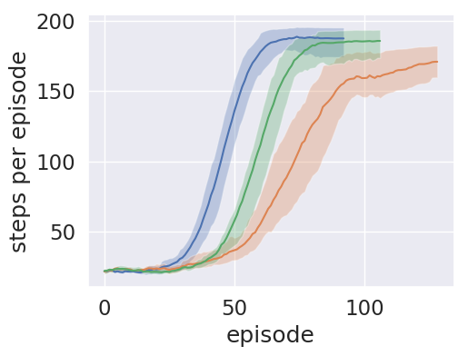
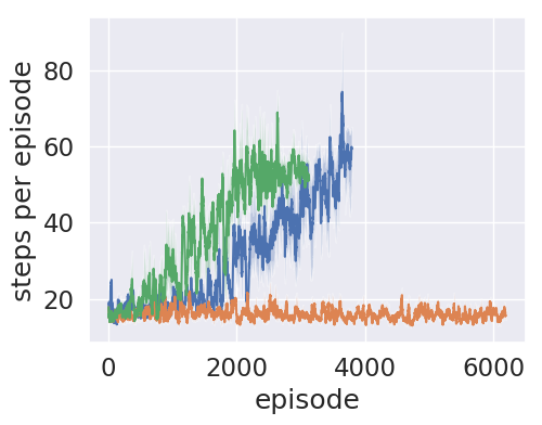
(b) CEM

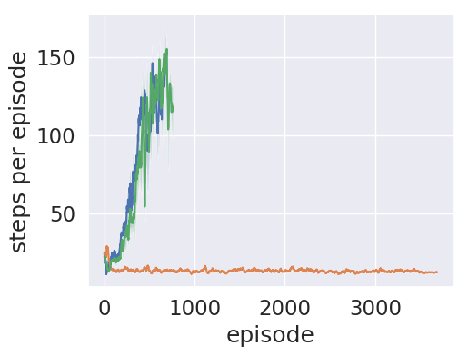
(c) SARSA

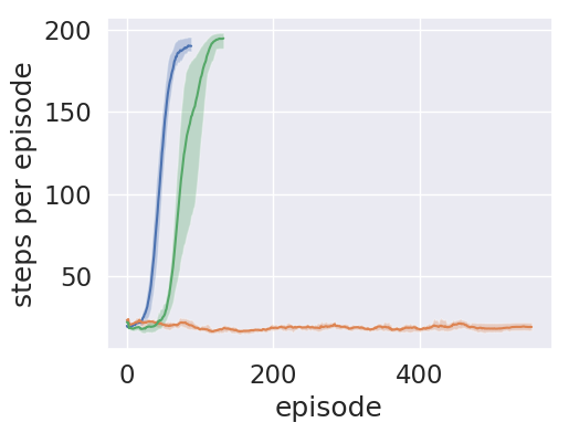
(d) DQN

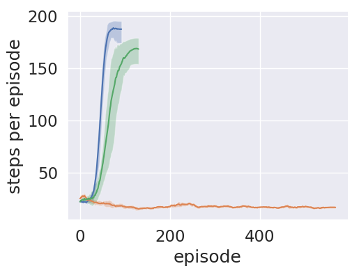
(e) DDQN

Figure 1: Learning curves from five RL algorithms on CartPole game with true rewards ($r$)  , noisy rewards ($\tilde{r}$)   and estimated surrogate rewards ($\dot{r}$)  ($\eta=1$)  . Note that ${\mathbf{C}}$ are unknown to the agents and each experiment is repeated 10 times with different random seeds. We plotted 10% to 90% percentile area with its mean highlighted. Full results are in Appendix D (Figure 6).

$\omega=0.7$

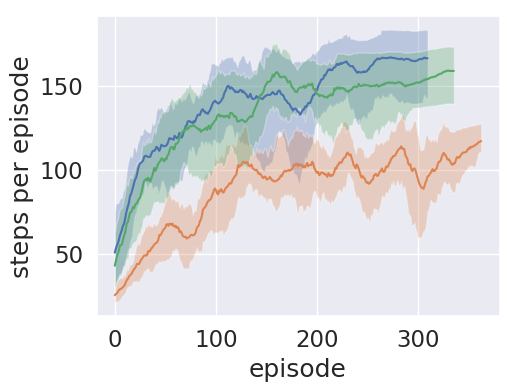
(a) $Q$-Learning

We present (Reward Robust RL) in Algorithm 1. Note that the algorithm is rather generic, and we can plug in any exisitng RL algorithm into our reward robust one, with only changes in replacing the rewards with our estimated surrogate rewards.

Experimental Results

In this section, we conduct extensive experiments to evaluate the noisy reward robust RL mechanism with different games, under various noise settings. Due to the space limit, more experimental results can be found in Appendix D.

Experimental Setup

Environments and RL Algorithms

To fully test the performance under different environments, we evaluate the proposed robust reward RL method on two classic control games (CartPole, Pendulum) and seven Atari 2600 games (AirRaid, Alien, Carnival, MsPacman, Pong, Phoenix, Seaquest), which encompass a large variety of environments, as well as rewards. Specifically, the rewards could be unary (CartPole), binary (most of Atari games), multivariate (Pong) and even continuous (Pendulum). A set of state-of-the-art RL algorithms are experimented with, while training under different amounts of noise (See Table 3). For each game and algorithm, unless otherwise stated, three policies are trained with different random initialization to decrease the variance.

$\omega=0.3$ $\omega=0.7$

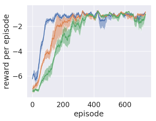
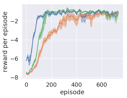
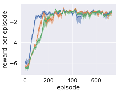
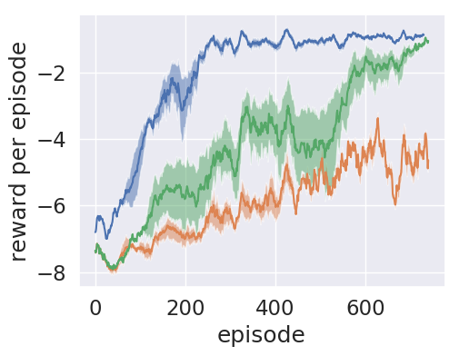
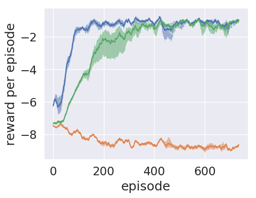
(a) DDPG (symmetric)

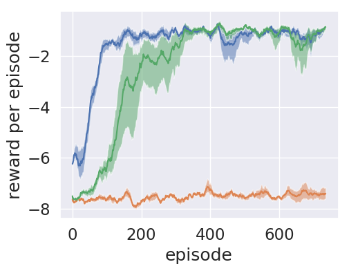
(b) DDPG (rand-one)

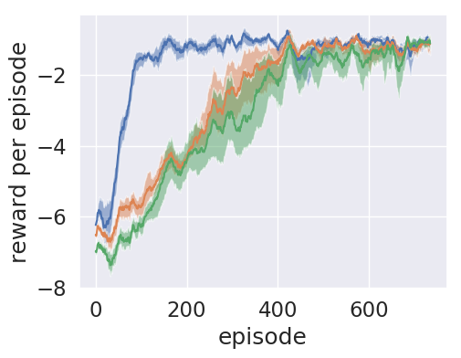
(c) DDPG (rand-all)

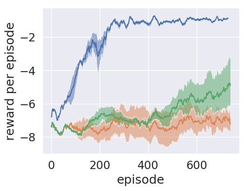
(d) NAF (rand-all)

Figure 2: Learning curves from DDPG and NAF on Pendulum game with true rewards ($r$)  , noisy rewards ($\tilde{r}$)   and surrogate rewards ($\hat{r}$) ($\eta=1$)  . Both symmetric and asymmetric noise are conduced in the experiments and each experiment is repeated 3 times with different random seeds. Full results are in Appendix D (Figure 9).

Reward Post-Processing

For each game and RL algorithm, we test the performance for learning with true rewards, noisy rewards and surrogate rewards. Both symmetric and asymmetric noise settings with different noise levels are tested. For symmetric noise, the confusion matrices are symmetric. As for asymmetric noise, two types of random noise are tested: 1) rand-one, each reward level can only be perturbed into another reward; 2) rand-all, each reward could be perturbed to any other reward, via adding a random noise matrix. To measure the amount of noise w.r.t confusion matrices, we define the weight of noise $\omega$ in Appendix B. The larger $\omega$ is, the higher the noise rates are.

Robustness Evaluation

CartPole

The goal in CartPole is to prevent the pole from falling by controlling the cart’s direction and velocity. The reward is $+1$ for every step taken, including the termination step. When the cart or pole deviates too much or the episode length is longer than 200, the episode terminates. Due to the unary reward $\{+1\}$ in CartPole, a corrupted reward $-1$ is added as the unexpected error ($e_{-}=0$). As a result, the reward space $\mathcal{R}$ is extended to $\{+1,-1\}$. Five algorithms $Q$-Learning (?), CEM (?), SARSA (?), DQN (?) and DDQN (?) are evaluated.

Table 1: Average scores of various RL algorithms on CartPole and Pendulum with noisy rewards ($\tilde{r}$) and surrogate rewards under known ($\hat{r}$) or estimated ($\dot{r}$) noise rates. Note that the results for last two algorithms DDPG (rand-one) $\&$ NAF (rand-all) are on Pendulum, but the others are on CartPole.

Noise Rate	Reward	$Q$-Learn	CEM	SARSA	DQN	DDQN	DDPG	NAF
$\omega=0.1$	$\tilde{r}$	170.0	98.1	165.2	187.2	187.8	-1.03	-4.48
	$\hat{r}$	165.8	108.9	173.6	200.0	181.4	-0.87	-0.89
	$\dot{r}$	181.9	99.3	171.5	200.0	185.6	-0.90	-1.13
$\omega=0.3$	$\tilde{r}$	134.9	28.8	144.4	173.4	168.6	-1.23	-4.52
	$\hat{r}$	149.3	85.9	152.4	175.3	198.7	-1.03	-1.15
	$\dot{r}$	161.1	82.2	159.6	186.7	200.0	-1.05	-1.36
$\omega=0.7$	$\tilde{r}$	56.6	19.2	12.6	17.2	11.8	-8.76	-7.35
	$\hat{r}$	177.6	87.1	151.4	185.8	195.2	-1.09	-2.26
	$\dot{r}$	172.1	83.0	174.4	189.3	191.3	–	–

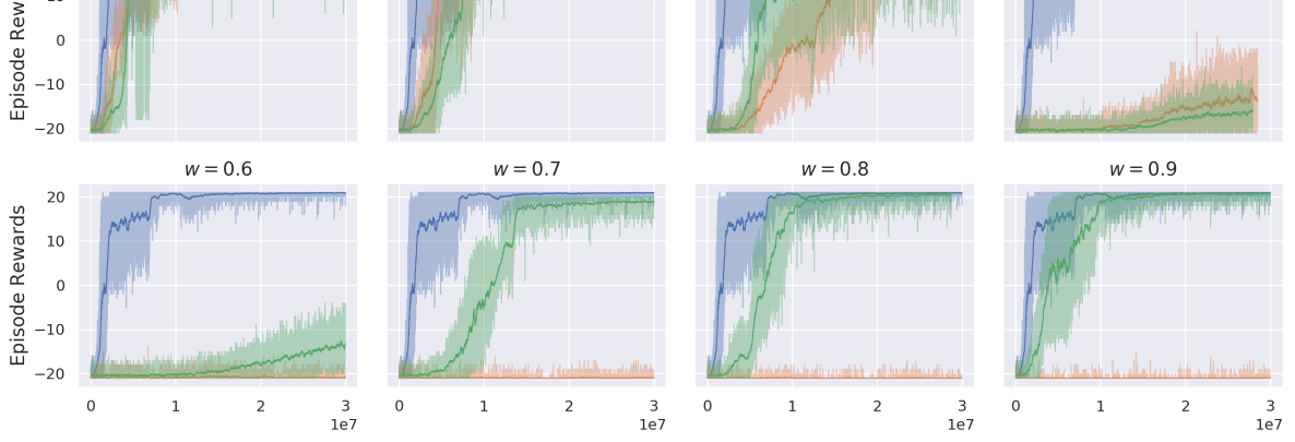
Figure 3: Learning curves from PPO on Pong-v4 game with true rewards ($r$)  , noisy rewards ($\tilde{r}$)   and surrogate rewards ($\eta=1$) ($\hat{r}$)  . The noise rate $\omega$ increases from 0.6 to 0.9, with a step of 0.1. Full results are in Appendix D (Figure 12).

Table 2: Average scores of PPO on five selected games with noisy rewards ($\tilde{r}$) and surrogate rewards under known ($\hat{r}$) or estimated ($\dot{r}$) noise rates.

Noise Rate	Reward	Lift ($\uparrow$)	Alien	Carnival	Phoenix	MsPacman	Seaquest
$\omega=0.1$	$\tilde{r}$	–	1835.1	1239.3	4609.0	1709.1	849.2
	$\hat{r}$	70.4%$\uparrow$	1737.0	3966.8	7586.4	2547.3	1610.6
	$\dot{r}$	84.6%$\uparrow$	2844.1	5515.0	5668.8	2294.5	2333.9
$\omega=0.3$	$\tilde{r}$	–	538.2	919.9	2600.3	1109.6	408.7
	$\hat{r}$	119.8%$\uparrow$	1668.6	4220.1	4171.6	1470.3	727.8
	$\dot{r}$	80.8%$\uparrow$	1542.9	4094.3	2589.1	1591.2	262.4
$\omega=0.7$	$\tilde{r}$	–	495.2	380.3	126.5	491.6	0.0
	$\hat{r}$	757.4%$\uparrow$	1805.9	4088.9	4970.4	1447.8	492.5
	$\dot{r}$	648.9%$\uparrow$	1618.0	4529.2	2792.1	1916.7	328.5

$\omega=0.9$

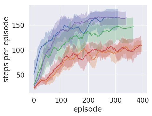
(a) $Q$-Learning

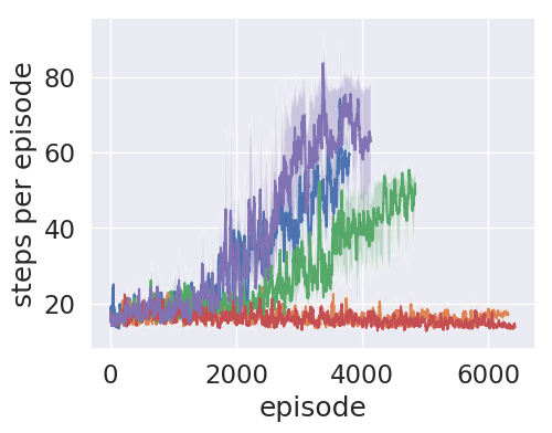
(b) CEM

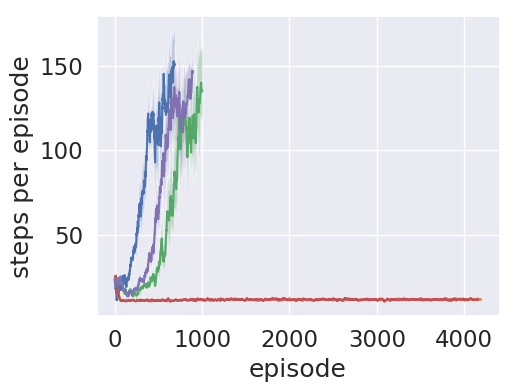
(c) SARSA

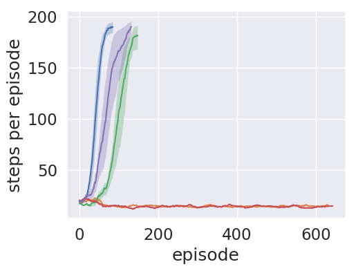
(d) DQN

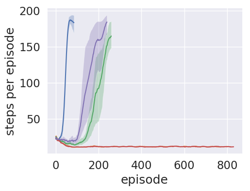
(e) DDQN

Figure 4: Learning curves from five reward robust RL algorithms on CartPole game with true rewards ($r$)  , noisy rewards ($\tilde{r}$)  , sample-mean noisy rewards  , estimated surrogate rewards ($\dot{r}$)   and sample-mean estimated surrogate rewards  . Full results are in Appendix D (Figure 8).

In Figure 1, we show that our estimator successfully produces meaningful surrogate rewards that adapt the underlying RL algorithms to the noisy settings, without any assumption of the true distribution of rewards. With the noise rate increasing (from 0.1 to 0.9), the models with noisy rewards converge slower due to larger biases. However, we observe that the models (DQN and DDQN) always converge to the best score 200 with the help of surrogate rewards.

In some circumstances (slight noise - see Figure 1(b), 1(c)), the surrogate rewards even lead to faster convergence. This points out an interesting observation: learning with surrogate reward sometimes even outperforms the case with observing the true reward. We conjecture that the way of adding noise and then removing the bias (or moderate noise) introduces implicit exploration. This may also imply why some algorithms with estimated confusion matrices $\tilde{{\mathbf{C}}}$ leads to better results than with known ${\mathbf{C}}$ in some cases (Table 1).

Pendulum

The goal in Pendulum is to keep a frictionless pendulum standing up. Different from the CartPole setting, the rewards in pendulum are continuous: $r\in(-16.28,0.0]$. The closer the reward is to zero, the better performance the model achieves. For simplicity, we firstly discretized $(-17,0]$ into 17 intervals: $(-17,-16],(-16,-15],\cdots,(-1,0]$, with its value approximated using its maximum point. After the quantization step, the surrogate rewards can be estimated using multi-outcome extensions.

We experiment two popular algorithms, DDPG (?) and NAF (?) in this game. In Figure 2, both algorithms perform well with surrogate rewards under different amounts of noise. In most cases, the biases were corrected in the long-term, even when the amount of noise is extensive (e.g., $\omega=0.7$). The quantitative scores on CartPole and Pendulum are given in Table 1, where the scores are averaged based on the last 30 episodes. Our reward robust method is able to achieve good scores consistently.

Atari

We validate our algorithm on seven Atari 2600 games using the state-of-the-art algorithm PPO (?). The games are chosen to cover a variety of environments. The rewards in the Atari games are clipped into $\{-1,0,1\}$. We leave the detailed settings to Appendix B.

Results for PPO on Pong-v4 in symmetric noise setting are presented in Figure 3. More results on other Atari games and noise settings are given in Appendix D. Similar to previous results, our surrogate estimator performs consistently well and helps PPO converge to the optimal policy. Table 2 shows the average scores of PPO on five selected Atari games with different amounts of noise (symmetric $\&$ asymmetric). In particular, when the noise rates $e_{+}=e_{-}>0.3$, agents with surrogate rewards obtain significant amounts of improvements in average scores. For the cases with unknown ${\mathbf{C}}$ ($\dot{r}$ in Table 2), due to the large state-space (image-input) in confusion matrix estimation, we embed and consider the adjacent frames within a batch as the same state and set the memory size for states as 1,000. Please refer to Appendix B for details.

Compatible with Variance Reduction Techniques

As illustrated in Theorem 3, our surrogate rewards introduce larger variance while conducting unbiased estimation, which are likely to decrease the stability of RL algorithms. Apart from the linear combination idea (a linear trade-off), some variance reduction techniques in statistics (e.g., correlated sampling) can also be applied to our method. Specially, ? proposed to use a reward estimator to compensate for stochastic corrupted-reward signals. It is worthy to notice that their method is designed for variance reduction under zero-mean noises, which is no longer efficacious in more general perturbed-reward setting. However, it is potential to integrate their method with our robust-reward RL framework because surrogate rewards provide unbiasedness guarantee.

To verify this idea, we repeated the experiments of Cartpole but included variance reduction step for estimated surrogate rewards. Following ?, we adopted sample mean as a simple approximator during the training and set sequence length as $100$. As shown in Figure 4, the models with only variance reduction technique (red lines) suffer from huge regrets, and in general do not converge to the optimal policies. Nevertheless, the variance reduction step helps surrogate rewards (purple lines) to achieve faster convergence or better performance in multiple cases. Similarly, Table 4 in Appendix C provides quantitative results which show that our surrogate reward benefits from variance reduction techniques (“ours + VRT”), especially when the noise rate is high.

Conclusions

Improving the robustness of RL in the settings with perturbed and noisy rewards is important given the fact that such noises are common when exploring a real-world scenario, such as sensor errors. In addition, in adversarial environments, perturbed reward could be leveraged Different robust RL algorithms have been proposed but they either only focus on the noisy observations or need strong assumption on the unbiased noise distribution for observed rewards. In this paper, we propose the first simple yet effective RL framework for dealing with biased noisy rewards. The convergence guarantee and finite sample complexity of $Q$-Learning (or its variant) with estimated surrogate rewards are provided. To validate the effectiveness of our approach, extensive experiments are conducted on OpenAI Gym, showing that surrogate rewards successfully rescue models from misleading rewards even at high noise rates. We believe this work will further shed light on exploring robust RL approaches under different noisy rewards observations in real-world environments.

Appendix A Proofs

Proof of Lemma 1.

For simplicity, we shorthand $\hat{r}(s_{t},a_{t},s_{t+1}),\tilde{r}(s_{t},a_{t},s_{t+1}),r(s_{t},a_{t},s_{t+1})$ as $\hat{r},\tilde{r},r$, and let $r_{+},r_{-},\hat{r}_{+},\hat{r}_{-}$ denote the general reward levels and corresponding surrogate ones:

$$\mathbb{E}_{\tilde{r}|r}(\hat{r})=\mathbb{P}_{\tilde{r}|r}(\hat{r}=\hat{r}_{-})\hat{r}_{-}+\mathbb{P}_{\tilde{r}|r}(\hat{r}=\hat{r}_{+})\hat{r}_{+}.$$ (7)

When $r=r_{+}$, from the definition in Lemma 1:

$$\mathbb{P}_{\tilde{r}|r}(\hat{r}=\hat{r}_{-})=e_{+},~{}\mathbb{P}_{\tilde{r}|r}(\hat{r}=\hat{r}_{+})=1-e_{+}.$$

Taking the definition of surrogate rewards Eqn. (2) into Eqn. (7), we have

$$\mathbb{E}_{\tilde{r}|r}(\hat{r}) =e_{+}\cdot\hat{r}_{-}+(1-e_{+})\cdot\hat{r}_{+}$$

$$=e_{+}\cdot\frac{(1-e_{+})r_{-7}-e_{-}r_{+}}{1-e_{-}-e_{+}}+(1-e_{+})\cdot\frac{(1-e_{-})r_{+}-e_{+}r_{-}}{1-e_{-}-e_{+}}=r_{+}.$$

Similarly, when $r=r_{-}$, it also verifies $\mathbb{E}_{\tilde{r}|r}[\hat{r}(s_{t},a_{t},s_{t+1})]=r(s_{t},a_{t},s_{t+1}).$ ∎

Proof of Lemma 2.

The idea of constructing unbiased estimator is easily adapted to multi-outcome reward settings via writing out the conditions for the unbiasedness property (s.t. $\mathbb{E}_{\tilde{r}|r}[\hat{r}]=r.$). For simplicity, we shorthand $\hat{r}(\tilde{r}=R_{i})$ as $\hat{R}_{i}$ in the following proofs. Similar to Lemma 1, we need to solve the following set of functions to obtain $\hat{r}$:

$$\begin{cases}\begin{aligned} R_{0}&=c_{0,0}\cdot\hat{R}_{0}+c_{0,1}\cdot\hat{R}_{1}+\dots+c_{0,M-1}\cdot\hat{R}_{M-1}\\ R_{1}&=c_{1,0}\cdot\hat{R}_{0}+c_{1,1}\cdot\hat{R}_{1}+\dots+c_{1,M-1}\cdot\hat{R}_{M-1}\\ &\cdots\\ R_{M-1}&=c_{M-1,0}\cdot\hat{R}_{0}+c_{M-1,1}\cdot\hat{R}_{1}+\dots+c_{M-1,M-1}\cdot\hat{R}_{M-1}\end{aligned}\end{cases}$$

where $\hat{R}_{i}$ denotes the value of the surrogate reward when the observed reward is $R_{i}$. Define ${\mathbf{R}}:=\left[R_{0};R_{1};\cdots;R_{M-1}\right]$, and $\hat{{\mathbf{R}}}:=[\hat{R}_{0},\hat{R}_{1},...,\hat{R}_{M-1}]$, then the above equations are equivalent to: ${\mathbf{R}}={\mathbf{C}}\cdot\hat{{\mathbf{R}}}.$ If the confusion matrix ${\mathbf{C}}$ is invertible, we obtain the surrogate reward:

$$\hat{{\mathbf{R}}}={\mathbf{C}}^{-1}\cdot{\mathbf{R}}.$$

According to above definition, for any true reward level $R_{i},i=0,1,\cdots,M-1$, we have

$$\mathbb{E}_{\tilde{r}|r=R_{i}}[\hat{r}]=c_{i,0}\cdot\hat{R}_{0}+c_{i,1}\cdot\hat{R}_{1}+\dots+c_{i,M-1}\cdot\hat{R}_{M-1}=R_{i}.$$

∎

Furthermore, the probabilities for observing surrogate rewards can be written as follows:

$$\hat{\mathbf{P}} =\left[\hat{p}_{1},\hat{p}_{2},\cdots,\hat{p}_{M}\right]=\left[\sum_{j}p_{j}c_{j,1},\sum_{j}p_{j}c_{j,2},\cdots,\sum_{j}p_{j}c_{j,M}\right],$$

where $\hat{p}_{i}=\sum_{j}p_{j}c_{j,i}$, and $\hat{p}_{i}$, $p_{i}$ represent the probabilities of occurrence for surrogate reward $\hat{R}_{i}$ and true reward $R_{i}$ respectively.

Corollary 1.

Let $\hat{p}_{i}$ and $p_{i}$ denote the probabilities of occurrence for surrogate reward $\hat{r}(\tilde{r}=R_{i})$ and true reward $R_{i}$. Then the surrogate reward satisfies,

$$\sum_{s_{t+1}\in\mathcal{S}}\mathbb{P}_{a}(s_{t},s_{t+1})r(s_{t},a,s_{t+1})=\sum_{j}p_{j}R_{j}=\sum_{j}\hat{p}_{j}\hat{R}_{j}.$$ (8)

Proof of Corollary 1.

From Lemma 2, we have,

$$\sum_{s_{t+1}\in\mathcal{S}}\mathbb{P}_{a}(s_{t},s_{t+1})r(s_{t},a,s_{t+1})=\sum_{s_{t+1}\in\mathcal{S};R_{j}\in\mathcal{R}}\mathbb{P}_{a}(s_{t},s_{t+1},R_{j})R_{j}$$

$$=\sum_{R_{j}\in\mathcal{R}}\sum_{s_{t+1}\in\mathcal{S}}\mathbb{P}_{a}(s_{t},s_{t+1})R_{j}=\sum_{R_{j}\in\mathcal{R}}p_{j}R_{j}=\sum_{j}p_{j}R_{j}.$$

Consequently,

$$\sum_{j}\hat{p}_{j}\hat{R}_{j} =\sum_{j}\sum_{k}p_{k}c_{k,j}\hat{R}_{j}=\sum_{k}p_{k}\sum_{j}c_{k,j}\hat{R}_{j}$$

$$=\sum_{k}p_{k}R_{k}=\sum_{s_{t+1}\in\mathcal{S}}\mathbb{P}_{a}(s_{t},s_{t+1})r(s_{t},a,s_{t+1}).$$

∎

To establish Theorem 1, we need an auxiliary result (Lemma 3) from stochastic process approximation, which is widely adopted for the convergence proof for $Q$-Learning (?; ?).

Lemma 3.

The random process $\{\Delta_{t}\}$ taking values in $\mathbb{R}^{n}$ and defined as

$$\Delta_{t+1}(x)=(1-\alpha_{t}(x))\Delta_{t}(x)+\alpha_{t}(x)F_{t}(x)$$

converges to zero w.p.1 under the following assumptions:

• $0\leq\alpha_{t}\leq 1$, $\sum_{t}\alpha_{t}(x)=\infty$ and $\sum_{t}\alpha_{t}(x)^{2}<\infty$;

• $||\mathbb{E}\left[F_{t}(x)|\mathcal{F}_{t}\right]||_{W}\leq\gamma||\Delta_{t}||$, with $\gamma<1$;

• ${\textbf{var}}\left[F_{t}(x)|\mathcal{F}_{t}\right]\leq C(1+||\Delta_{t}||^{2}_{W})$, for $C>0$.

Here $\mathcal{F}_{t}=\{\Delta_{t},\Delta_{t-1},\cdots,F_{t-1}\,\cdots,\alpha_{t},\cdots\}$ stands for the past at step $t$, $\alpha_{t}(x)$ is allowed to depend on the past insofar as the above conditions remain valid. The notation $||\cdot||_{W}$ refers to some weighted maximum norm.

Proof of Lemma 3.

See previous literature (?; ?). ∎

Proof of Theorem 1.

For simplicity, we abbreviate $s_{t}$, $s_{t+1}$, $Q_{t}$, $Q_{t+1}$, $r_{t}$, $\hat{r}_{t}$ and $\alpha_{t}$ as $s$, $s^{\prime}$, $Q$, $Q^{\prime}$, $r$, $\hat{r}$, and $\alpha$, respectively.

Subtracting from both sides the quantity $Q^{\ast}(s,a)$ in Eqn. (4):

$$Q^{\prime}(s,a)-Q^{\ast}(s,a)= (1-\alpha)\left(Q(s,a)-Q^{\ast}(s,a)\right)+\alpha\left[\hat{r}+\gamma\max_{b\in\mathcal{A}}Q(s^{\prime},b)-Q^{\ast}(s,a)\right].$$

Let $\Delta_{t}(s,a)=Q(s,a)-Q^{\ast}(s,a)$ and $F_{t}(s,a)=\hat{r}+\gamma\max_{b\in\mathcal{A}}Q(s^{\prime},b)-Q^{\ast}(s,a)$.

$$\Delta_{t+1}(s^{\prime},a)=(1-\alpha)\Delta_{t}(s,a)+\alpha F_{t}(s,a).$$

In consequence,

$$\mathbb{E}\left[F_{t}(x)|\mathcal{F}_{t}\right] =\sum_{s^{\prime}\in\mathcal{S};\hat{r}\in\mathcal{R}}\mathbb{P}_{a}(s,s^{\prime},\hat{r})\left[\hat{r}+\gamma\max_{b\in\mathcal{A}}Q(s^{\prime},b)\right]-Q^{\ast}(s,a)$$

$$=\sum_{s^{\prime}\in\mathcal{S};\hat{r}\in\mathcal{R}}\mathbb{P}_{a}(s,s^{\prime},\hat{r})\hat{r}+\sum_{s^{\prime}\in\mathcal{S}}\mathbb{P}_{a}(s,s^{\prime})\left[\gamma\max_{b\in\mathcal{A}}Q(s^{\prime},b)-r-\gamma\max_{b\in\mathcal{A}}Q^{\ast}(s^{\prime},b)\right]$$

$$=\sum_{s^{\prime}\in\mathcal{S};\hat{r}\in\mathcal{R}}\mathbb{P}_{a}(s,s^{\prime},\hat{r})\hat{r}-\sum_{s^{\prime}\in\mathcal{S}}\mathbb{P}_{a}(s,s^{\prime})r+\sum_{s^{\prime}\in\mathcal{S}}\mathbb{P}_{a}(s,s^{\prime})\gamma\left[\max_{b\in\mathcal{A}}Q(s^{\prime},b)-\max_{b\in\mathcal{A}}Q^{\ast}(s^{\prime},b)\right]$$

$$=\sum_{j}\hat{p}_{j}\hat{r}_{j}-\sum_{s^{\prime}\in\mathcal{S}}\mathbb{P}_{a}(s,s^{\prime})r+\sum_{s^{\prime}\in\mathcal{S}}\mathbb{P}_{a}(s,s^{\prime})\gamma\left[\max_{b\in\mathcal{A}}Q(s^{\prime},b)-\max_{b\in\mathcal{A}}Q^{\ast}(s^{\prime},b)\right]$$

$$=\sum_{s^{\prime}\in\mathcal{S}}\mathbb{P}_{a}(s,s^{\prime})\gamma\left[\max_{b\in\mathcal{A}}Q(s^{\prime},b)-\max_{b\in\mathcal{A}}Q^{\ast}(s^{\prime},b)\right]$$

$$\leq\gamma\sum_{s^{\prime}\in\mathcal{S}}\mathbb{P}_{a}(s,s^{\prime})\max_{b\in\mathcal{A},s^{\prime}\in\mathcal{S}}\left\lvert Q(s^{\prime},b)-Q^{\ast}(s^{\prime},b)\right\rvert$$

$$=\gamma\sum_{s^{\prime}\in\mathcal{S}}\mathbb{P}_{a}(s,s^{\prime})||Q-Q^{\ast}||_{\infty}=\gamma||Q-Q^{\ast}||_{\infty}=\gamma||\Delta_{t}||_{\infty}.$$

Finally,

$${\mathbf{Var}}\left[F_{t}(x)|\mathcal{F}_{t}\right] =\mathbb{E}\Bigg{[}\bigg{(}\hat{r}+\gamma\max_{b\in\mathcal{A}}Q(s^{\prime},b)-\sum_{s^{\prime}\in\mathcal{S};\hat{r}\in\mathcal{R}}\mathbb{P}^{\prime}(s,s^{\prime},\hat{r})\left[\hat{r}+\gamma\max_{b\in\mathcal{A}}Q(s^{\prime},b)\right]\bigg{)}^{2}\Bigg{]}$$

$$={\mathbf{Var}}\left[\hat{r}+\gamma\max_{b\in\mathcal{A}}Q(s^{\prime},b)|\mathcal{F}_{t}\right]$$

.

Because $\hat{r}$ is bounded, it can be clearly verified that

$${\mathbf{Var}}\left[F_{t}(x)|\mathcal{F}_{t}\right]\leq C(1+||\Delta_{t}||^{2}_{W})$$

for some constant $C$. Then, due to the Lemma 3, $\Delta_{t}$ converges to zero w.p.1, i.e., $Q^{\prime}(s,a)$ converges to $Q^{\ast}(s,a)$. ∎

The procedure of Phased $Q$-Learning is described as Algorithm 2:

Algorithm 2 Phased $Q$-Learning

  Input: $G(\mathcal{M})$: generative model of $\mathcal{M}=(\mathcal{S},\mathcal{A},\mathcal{R},\mathcal{P},\gamma)$, $T$: number of iterations.

  Output: $\hat{V}(s)$: value function, $\hat{\pi}(s,t)$: policy function.

  Set $\hat{V}_{T}(s)=0$

  for $t=T-1,\cdots,0$ do

     Calling $G(\mathcal{M})$ $m$ times for each state-action pair.

$$\hat{\mathbb{P}}_{a}(s_{t},s_{t+1})=\frac{\#[(s_{t},a_{t})\to s_{t+1}]}{m}$$

     Set

$$\hat{V}(s_{t}) =\max_{a\in\mathcal{A}}\sum_{s_{t+1}\in\mathcal{S}}\hat{\mathbb{P}}_{a}(s_{t},s_{t+1})\left[r_{t}+\gamma\hat{V}(s_{t+1})\right]$$

$$\hat{\pi}(s,t) =\operatorname*{arg\,max}_{a\in\mathcal{A}}\hat{V}(s_{t})$$

  end for

  return $\hat{V}(s)$ and $\hat{\pi}(s,t)$

Note that $\hat{\mathbb{P}}$ here is the estimated transition probability, which is different from $\mathbb{P}$ in Eqn. (8).

To obtain the sample complexity results, the range of our surrogate reward needs to be known. Assuming reward $r$ is bounded in $[0,R_{\max}]$, Lemma 4 below states that the surrogate reward is also bounded, when the confusion matrices are invertible:

Lemma 4.

Let $r\in[0,R_{\max}]$ be bounded, where $R_{\max}$ is a constant; suppose ${\mathbf{C}}_{M\times M}$, the confusion matrix, is invertible with its determinant denoting as $\mathrm{det}({\mathbf{C}})$. Then the surrogate reward satisfies

$$0\leq\left|\hat{r}\right|\leq\frac{M}{\mathrm{det}({\mathbf{C}})}R_{\max}.$$ (9)

Proof of Lemma 4.

From Eqn. (3), we have,

$$\hat{{\mathbf{R}}}={\mathbf{C}}^{-1}\cdot{\mathbf{R}}=\frac{\mathrm{adj}({\mathbf{C}})}{\mathrm{det}({\mathbf{C}})}\cdot{\mathbf{R}},$$

where $\mathrm{adj}({\mathbf{C}})$ is the adjugate matrix of ${\mathbf{C}}$; $\mathrm{det}({\mathbf{C}})$ is the determinant of ${\mathbf{C}}$. It is known from linear algebra that,

$$\mathrm{adj}({\mathbf{C}})_{ij}=(-1)^{i+j}\cdot{\mathbf{M}}_{ji},$$

where ${\mathbf{M}}_{ji}$ is the determinant of the $(M-1)\times(M-1)$ matrix that results from deleting row $j$ and column $i$ of ${\mathbf{C}}$. Therefore, ${\mathbf{M}}_{ji}$ is also bounded:

$${\mathbf{M}}_{ji}\leq\sum_{\sigma\in S_{n}}\left(\left|\mathrm{sgn}(\sigma)\right|\prod\limits_{m=1}c^{\prime}_{m,\sigma_{n}}\right)\leq\prod\limits_{m=0}^{M-1}\left(\sum\limits_{n=0}^{M-1}c_{m,n}\right)=1^{M}=1,$$

where the sum is computed over all permutations $\sigma$ of the set $\{0,1,\cdots,M-2\}$; $c^{\prime}$ is the element of ${\mathbf{M}}_{ji}$; $\mathrm{sgn}(\sigma)$ returns a value that is $+1$ whenever the reordering given by $\sigma$ can be achieved by successively interchanging two entries an even number of times, and $-1$ whenever it can not.

Consequently,

$$\left|\hat{R}_{i}\right|=\frac{\sum_{j}\left|\mathrm{adj}({\mathbf{C}})_{ij}\right|\cdot\left|R_{j}\right|}{\mathrm{det}({\mathbf{C}})}\leq\frac{M}{\mathrm{det}({\mathbf{C}})}\cdot R_{\max}.$$

∎

Proof of Theorem 2.

From Hoeffding’s inequality, we obtain:

$$P\left(\left|\sum_{s_{t+1}\in\mathcal{S}}\mathbb{P}_{a}(s_{t},s_{t+1})V_{t+1}^{\ast}(s_{t+1})-\sum_{s_{t+1}\in\mathcal{S}}\hat{\mathbb{P}}_{a}(s_{t},s_{t+1})V_{t+1}^{\ast}(s_{t+1})\right|\geq\epsilon\right)\leq 2\exp{\left(\frac{-2m\epsilon^{2}(1-\gamma)^{2}}{R_{\max}^{2}}\right)},$$

because $V_{t}(s_{t})$ is bounded within $\frac{R_{\max}}{1-\gamma}$. In the same way, $\hat{r}_{t}$ is bounded by $\frac{M}{\mathrm{det}({\mathbf{C}})}\cdot R_{\max}$ from Lemma 4. We then have,

$$P\left(\left|\sum_{\begin{subarray}{c}s_{t+1}\in\mathcal{S}\\ \hat{r}_{t}\in\mathcal{\hat{R}}\end{subarray}}\mathbb{P}_{a}(s_{t},s_{t+1},\hat{r}_{t})\hat{r}_{t}-\sum_{\begin{subarray}{c}s_{t+1}\in\mathcal{S}\\ \hat{r}_{t}\in\mathcal{\hat{R}}\end{subarray}}\hat{\mathbb{P}}_{a}(s_{t},s_{t+1},\hat{r}_{t})\hat{r}_{t}\right|\geq\epsilon\right)\leq 2\exp{\left(\frac{-2m\epsilon^{2}\mathrm{det}({\mathbf{C}})^{2}}{M^{2}R_{\max}^{2}}\right)}.$$

Further, due to the unbiasedness of surrogate rewards, we have

$$\sum_{s_{t+1}\in\mathcal{S}}\mathbb{P}_{a}(s_{t},s_{t+1})r_{t}=\sum_{s_{t+1}\in\mathcal{S};\hat{r}_{t}\in\mathcal{\hat{R}}}\mathbb{P}_{a}(s_{t},s_{t+1},\hat{r}_{t})\hat{r}_{t}.$$

As a result,

$$\left|V_{t}^{\ast}(s)-\hat{V}_{t}(s)\right| =\max_{a\in\mathcal{A}}\sum_{s_{t+1}\in\mathcal{S}}\mathbb{P}_{a}(s_{t},s_{t+1})\left[r_{t}+\gamma V_{t+1}^{\ast}(s_{t+1})\right]-\max_{a\in\mathcal{A}}\sum_{s_{t+1}\in\mathcal{S}}\hat{\mathbb{P}}_{a}(s_{t},s_{t+1})\left[\hat{r}_{t}+\gamma V_{t+1}^{\ast}(s_{t+1})\right]$$

$$\leq\epsilon_{1}+\gamma\max_{a\in\mathcal{A}}\left|\sum_{s_{t+1}\in\mathcal{S}}\mathbb{P}_{a}(s_{t},s_{t+1})V_{t+1}^{\ast}(s_{t+1})-\sum_{s_{t+1}\in\mathcal{S}}\hat{\mathbb{P}}_{a}(s_{t},s_{t+1})V_{t+1}^{\ast}(s_{t+1})\right|$$

$$\quad+\max_{a\in\mathcal{A}}\left|\sum_{s_{t+1}\in\mathcal{S}}\mathbb{P}_{a}(s_{t},s_{t+1})r_{t}-\sum_{s_{t+1}\in\mathcal{S};\hat{r}_{t}\in\mathcal{\hat{R}}}\mathbb{P}_{a}(s_{t},s_{t+1},\hat{r}_{t})\hat{r}_{t}\right|$$

$$\leq\gamma\max_{s\in\mathcal{S}}\left|V_{t+1}^{\ast}(s)-\hat{V}_{t+1}(s)\right|+\epsilon_{1}+\gamma\epsilon_{2}$$

In the same way,

$$\left|V_{t}(s)-\hat{V}_{t}(s)\right|\leq\gamma\max_{s\in\mathcal{S}}\left|V_{t+1}^{\ast}(s)-\hat{V}_{t+1}(s)\right|+\epsilon_{1}+\gamma\epsilon_{2}$$

Recursing the two equations in two directions ($0\to T$), we get

$$\max_{s\in\mathcal{S}}\left|V^{\ast}(s)-\hat{V}(s)\right| \leq(\epsilon_{1}+\gamma\epsilon_{2})+\gamma(\epsilon_{1}+\gamma\epsilon_{2})+\cdots+\gamma^{T-1}(\epsilon_{1}+\gamma\epsilon_{2})$$

$$=\frac{(\epsilon_{1}+\gamma\epsilon_{2})(1-\gamma^{T})}{1-\gamma}$$

$$\max_{s\in\mathcal{S}}\left|V(s)-\hat{V}(s)\right| \leq\frac{(\epsilon_{1}+\gamma\epsilon_{2})(1-\gamma^{T})}{1-\gamma}$$

Combining these two inequalities above we have:

$$\max_{s\in\mathcal{S}}\left|V^{\ast}(s)-V(s)\right|\leq 2\frac{(\epsilon_{1}+\gamma\epsilon_{2})(1-\gamma^{T})}{1-\gamma}\leq 2\frac{(\epsilon_{1}+\gamma\epsilon_{2})}{1-\gamma}.$$

Let $\epsilon_{1}=\epsilon_{2}$, so $\max_{s\in\mathcal{S}}\left|V^{\ast}(s)-V(s)\right|\leq\epsilon$ as long as

$$\epsilon_{1}=\epsilon_{2}\leq\frac{(1-\gamma)\epsilon}{2(1+\gamma)}.$$

For arbitrarily small $\epsilon$, by choosing $m$ appropriately, there always exists $\epsilon_{1}=\epsilon_{2}=\frac{(1-\gamma)\epsilon}{2(1+\gamma)}$ such that the policy error is bounded within $\epsilon$. That is to say, the Phased Q-Learning algorithm can converge to the near optimal policy within finite steps using our proposed surrogate rewards.

Finally, there are $|\mathcal{S}||\mathcal{A}|T$ transitions under which these conditions must hold, where $|\cdot|$ represent the number of elements in a specific set. Using a union bound, the probability of failure in any condition is smaller than

$$2|\mathcal{S}||\mathcal{A}|T\cdot\exp\left({-m\frac{\epsilon^{2}(1-\gamma)^{2}}{2(1+\gamma)^{2}}}\cdot\min\{(1-\gamma)^{2},\frac{\mathrm{det}({\mathbf{C}})^{2}}{M^{2}}\}\right).$$

We set the error rate less than $\delta$, and $m$ should satisfy that

$$m=O\left(\frac{1}{\epsilon^{2}(1-\gamma)^{2}\mathrm{det}({\mathbf{C}})^{2}}\log\frac{|\mathcal{S}||\mathcal{A}|T}{\delta}\right).$$

In consequence, after $m|\mathcal{S}||\mathcal{A}|T$ calls, which is, $O\left(\frac{|\mathcal{S}||\mathcal{A}|T}{\epsilon^{2}(1-\gamma)^{2}\mathrm{det}({\mathbf{C}})^{2}}\log\frac{|\mathcal{S}||\mathcal{A}|T}{\delta}\right)$, the value function converges to the optimal one for every state $s$, with probability greater than $1-\delta$. ∎

The above bound is for discounted MDP setting with $0\leq\gamma<1$. For undiscounted setting $\gamma=1$, since the total error (for entire trajectory of $T$ time-steps) has to be bounded by $\epsilon$, therefore, the error for each time step has to be bounded by $\frac{\epsilon}{T}$. Repeating our anayslis, we obtain the following upper bound:

$$O\left(\frac{|\mathcal{S}||\mathcal{A}|T^{3}}{\epsilon^{2}\mathrm{det}({\mathbf{C}})^{2}}\log\frac{|\mathcal{S}||\mathcal{A}|T}{\delta}\right).$$

Proof of Theorem 3.

$$\mathbf{Var}(\hat{r})-\mathbf{Var}(r) =\mathbb{E}\left[(\hat{r}-\mathbb{E}[\hat{r}])^{2}\right]-\mathbb{E}\left[\left({r}-\mathbb{E}[{r}]\right)^{2}\right]$$

$$=\mathbb{E}[\hat{r}^{2}]-\mathbb{E}[\hat{r}]^{2}+\mathbb{E}[{r}^{2}]-\mathbb{E}[{r}]^{2}$$

$$=\sum_{j}\hat{p}_{j}\hat{R_{j}}^{2}-\left(\sum_{j}\hat{p}_{j}\hat{R}_{j}\right)^{2}-\left[\sum_{j}{p}_{j}{R_{j}}^{2}-\left(\sum_{j}{p}_{j}{R}_{j}\right)^{2}\right]$$

$$=\sum_{j}\hat{p}_{j}\hat{R_{j}}^{2}-\sum_{j}{p}_{j}{R_{j}}^{2}$$

$$=\sum_{j}\sum_{i}p_{i}c_{i,j}\hat{R_{j}}^{2}-\sum_{j}p_{j}\left(\sum_{i}c_{j,i}\hat{R_{i}}\right)^{2}$$

$$=\sum_{j}p_{j}\left(\sum_{i}c_{j,i}\hat{R_{i}}^{2}-\left(\sum_{i}c_{j,i}\hat{R_{i}}\right)^{2}\right).$$

Using the Cauchy–Schwarz inequality,

$$\sum_{i}c_{j,i}\hat{R_{i}}^{2}=\sum_{i}\sqrt{c_{j,i}}^{2}\cdot\sum_{i}\left(\sqrt{c_{j,i}}\hat{R_{i}}\right)^{2}\geq\left(\sum_{i}c_{j,i}\hat{R_{i}}\right)^{2}.$$

So we get,

$$\mathbf{Var}(\hat{r})-\mathbf{Var}(r)\geq 0.$$

In addition,

$$\mathbf{Var}(\hat{r}) =\sum_{j}\hat{p}_{j}\hat{R_{j}}^{2}-\left(\sum_{j}\hat{p}_{j}\hat{R}_{j}\right)^{2}\leq\sum_{j}\hat{p}_{j}\hat{R_{j}}^{2}$$

$$\leq\sum_{j}\hat{p}_{j}\frac{M^{2}}{\mathrm{det}({\mathbf{C}})^{2}}\cdot R_{\max}^{2}=\frac{M^{2}}{\mathrm{det}({\mathbf{C}})^{2}}\cdot R_{\max}^{2}.$$

∎

Appendix B Experimental Setup

We set up our experiments within the popular OpenAI baselines (?) and keras-rl (?) framework. Specifically, we integrate the algorithms and interact with OpenAI Gym (?) environments (Table 3).

Table 3: RL algorithms utilized in the robustness evaluation.

Environment	RL Algorithm
CartPole	$Q$-Learning (?)
	CEM (?)
	SARSA (?)
	DQN (?; ?)
	DDQN (?)
Pendulum	DDPG (?)
	NAF (?)
Atari Games	PPO (?)

RL Algorithms

A set of state-of-the-art reinforcement learning algorithms are experimented with while training under different amounts of noise, including $Q$-Learning (?; ?), Cross-Entropy Method (CEM) (?), Deep SARSA (?), Deep $Q$-Network (DQN) (?; ?; ?), Dueling DQN (DDQN) (?), Deep Deterministic Policy Gradient (DDPG) (?), Continuous DQN (NAF) (?) and Proximal Policy Optimization (PPO) (?) algorithms. For each game and algorithm, three policies are trained based on different random initialization to decrease the variance in experiments.

Post-Processing Rewards

We explore both symmetric and asymmetric noise of different noise levels. For symmetric noise, the confusion matrices are symmetric, which means the probabilities of corruption for each reward choice are equivalent. For instance, a confusion matrix

$$\mathbf{C}=\begin{bmatrix}0.8&0.2\\ 0.2&0.8\end{bmatrix}$$

says that $r_{1}$ could be corrupted into $r_{2}$ with a probability of 0.2 and so does $r_{2}$ (weight = 0.2).

As for asymmetric noise, two types of random noise are tested: 1) rand-one, each reward level can only be perturbed into another reward; 2) rand-all, each reward could be perturbed to any other reward. To measure the amount of noise w.r.t confusion matrices, we define the weight of noise as follows:

$${\mathbf{C}}=(1-\omega)\cdot{\mathbf{I}}+\omega\cdot{\mathbf{N}},~{}\omega\in[0,1],$$

where $\omega$ controls the weight of noise; ${\mathbf{I}}$ and ${\mathbf{N}}$ denote the identity and noise matrix respectively. Suppose there are $M$ outcomes for true rewards, ${\mathbf{N}}$ writes as:

$${\mathbf{N}}=\begin{bmatrix}n_{0,0}&n_{0,1}&\cdots&n_{0,M-1}\\ \cdots&\cdots&\cdots&\cdots\\ n_{M-1,0}&n_{M-1,1}&\cdots&n_{M-1,M-1}\\ \end{bmatrix},$$

where for each row $i$, 1) rand-one: randomly choose $j$, s.t $n_{i,j}=1$ and $n_{i,k}\neq 0$ if $k\neq j$; 2) rand-all: generate $M$ random numbers that sum to 1, i.e., $\sum_{j}n_{i,j}=1$. For the simplicity, for symmetric noise, we choose ${\mathbf{N}}$ as an anti-identity matrix. As a result, $c_{i,j}=0$, if $i\neq j$ or $i+j\neq M$.

Perturbed-Reward MDP Example

To obtain an intuitive view of the reward perturbation model, where the observed rewards are generated based on a reward confusion matrix, and meanwhile evaluate our estimation algorithm’s robustness to time-variant noise, we constructed a simple MDP and evaluated the performance of robust reward $Q$-Learning (Algorithm 1) on different noise ratios (both symmetric and asymmetric). The finite MDP is formulated as Figure 5(a): when the agent reaches state 5, it gets an instant reward of $r_{+}=1$, otherwise a zero reward $r_{-}=0$. During the explorations, the rewards are perturbed according to the confusion matrix ${\mathbf{C}}_{2\times 2}=\left[1-e_{-},e_{-};e_{+},1-e_{+}\right]$.

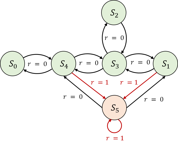
(a) Finite MDP (six-state)

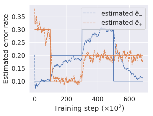
(b) Estimation process in time-variant noise

Figure 5: Perturbed-Reward MDP Example

For time-variant noise, we generated varying amount of noise at different training stages: 1) $e_{-}=0.1,e_{+}=0.3$ ($0$ to $1e^{4}$ steps); 2) $e_{-}=0.2,e_{+}=0.1$ ($1e^{4}$ to $3e^{4}$ steps); 3) $e_{-}=0.3,e_{+}=0.2$ ($3e^{4}$ to $5e^{4}$ steps); 4) $e_{-}=0.1,e_{+}=0.2$ ($5e^{4}$ to $7e^{4}$ steps). In Figure 5(b), we show that Algorithm 1 is robust against time-variant noise, which dynamically adjusts the estimated $\tilde{{\mathbf{C}}}$ after the noise distribution changes. Note that we set a maximum memory size for collected noisy rewards to let the agents only learn with recent observations.

Training Details

CartPole and Pendulum

The policies use the default network from keras-rl framework. which is a five-layer fully connected network. There are three hidden layers, each of which has 16 units and followed by a rectified nonlinearity. The last output layer is activated by the linear function. For CartPole, We trained the models using Adam optimizer with the learning rate of $1e^{-3}$ for 10,000 steps. The exploration strategy is Boltzmann policy. For DQN and Dueling-DQN, the update rate of target model and the memory size are $1e^{-2}$ and $50,000$. For Pendulum, We trained DDPG and NAF using Adam optimizer with the learning rate of $5e^{-4}$ for $150,000$ steps. the update rate of target model and the memory size are $1e^{-3}$ and $100,000$.

Atari Games

We adopt the pre-processing steps as well as the network architecture from  (?). Specifically, the input to the network is $84\times 84\times 4$, which is a concatenation of the last 4 frames and converted into $84\times 84$ gray-scale. The network comprises three convolutional layers and two fully connected layers. The kernel size of three convolutional layer are $8\times 8$ with stride 4 (32 filters), $4\times 4$ with stride 2 (64 filters) and $3\times 3$ with stride 1 (64 filters), respectively. Each hidden layer is followed by a rectified nonlinearity. Except for Pong where we train the policies for $3e^{7}$ steps, all the games are trained for $5e^{7}$ steps with the learning rate of $3e^{-4}$. Note that the rewards in the Atari games are discrete and clipped into $\{-1,0,1\}$. Except for Pong game, in which $r=-1$ means missing the ball hit by the adversary, the agents in other games attempt to get higher scores in the episode with binary rewards $0$ and $1$.

Discretization for Continuous States

To apply proposed estimation algorithm to continuous-state MDPs, we adopt a discretization procedure similar to the pre-processing of continuous rewards As stated before, there is a also trade-off between the quantization error as well as the estimation complexity. However, in practice, we found that the estimation step is highly robust to the quantization level.

For Cartpole, the observations (states) are speed and velocity of the cart, and we discretized them into $8~{}\text{(speeds)}\times 10~{}\text{(velocity)}=80$ independent states for collecting noisy rewards for each state-action pair. In inverted Pendulum swingup problem, the states ($\cos\theta\in[-1.0,1.0];\sin\theta\in[-1.0,1.0];d\theta/dt\in[-8.0,+8.0]$, $\theta$ denotes the rotation degree of pendulum) are discretized into $20~{}(\cos\theta)\times 20~{}(sin\theta)\times 40~{}(d\theta/dt)=16,000$ states. When the state-space is high-dimensional (e.g., the image inputs for Atari games), we propose a batch-based adjacency embedding policy. In particular, we embedded a batch (32) of adjacent image observations as one single state. For the consideration of time dependency and efficiency, we set a “state queue” which only records the noisy rewards for the latest 1,000 states. The confusion matrices are re-estimated based on current collections of observed noisy rewards every 100 steps.

Appendix C Estimation of Confusion Matrices

Reward Robust RL Algorithms

As stated in proposed reward robust RL framework, the confusion matrix can be estimated dynamically based on the aggregated answers, similar to previous literature in supervised learning (?). To get a concrete view, we take $Q$-Learning for an example, and the algorithm is called Reward Robust $Q$-Learning (Algorithm 3). Note that is can be extended to other RL algorithms by plugging confusion matrix estimation steps and the computed surrogate rewards, as shown in the experiments (Figure 6).

Algorithm 3 Reward Robust $Q$-Learning

  Input: $\mathcal{\tilde{M}}=(\mathcal{S},\mathcal{A},\mathcal{\tilde{R}},\mathcal{P},\gamma)$: MDP with corrupted reward channel $T$: transition function $T:\mathcal{S}\times\mathcal{A}\rightarrow\mathcal{S}$ $D_{\min}\in\mathbb{N}$: lower bound of collected noisy rewards (to collect enough noisy copies)$\alpha\in(0,1)$: learning rate in the update rule $\eta\in(0,1)$: weight of unbiased surrogate reward $\tilde{R}(s,a)$: set of observed rewards with a maximum size $D_{\max}$ when the state-action pair is $(s,a)$.

  Output: $Q(s,a)$: value function; $\pi(s)$: policy function

  Initialize $Q$: $\mathcal{S}\times\mathcal{A}\rightarrow\mathbb{R}$ arbitrarily

  Set confusion matrix $\tilde{{\mathbf{C}}}$ as identity matrix ${\mathbf{I}}$

  while $Q$ is not converged do

     Start in state $s\in\mathcal{S}$

     while $s$ is not terminal do

        Calculate $\pi$ according to $Q$ and exploration strategy

        $a\leftarrow\pi(s)$; $s^{\prime}\leftarrow T(s,a)$

        Observe noisy reward $\tilde{r}(s,a)$ and add it to $\tilde{R}(s,a)$

        if $\sum_{(s,a)}|\tilde{R}(s,a)|\geq D_{\min}$ then

           Get predicted true reward $\bar{r}(s,a)$ using majority voting in every $\tilde{R}(s,a)$ (using Eqn. 5)

           Re-estimate confusion matrix $\tilde{{\mathbf{C}}}$ based on $\tilde{r}(s,a)$ and $\bar{r}(s,a)$ (using Eqn. 6)

        end if

        Obtain surrogate reward $\dot{r}(s,a)$ using ${\mathbf{R}}_{proxy}=(1-\eta)\cdot{{\mathbf{R}}}+\eta\cdot{\mathbf{C}}^{-1}{{\mathbf{R}}}$

        $Q(s,a)\leftarrow(1-\alpha)\cdot Q(s,a)+\alpha\cdot\left(\hat{r}(s,a)+\gamma\cdot\max_{a^{\prime}}Q(s^{\prime},a^{\prime})\right)$

        $s\leftarrow s^{\prime}$

     end while

  end while

  return $Q(s,a)$ and $\pi(s)$

State-Dependent Perturbed Reward

In previous sections, to let our presentation stay focused, we consider the state-independent perturbed reward environments, which share the same confusion matrix for all states. In other words, the noise for different states is generated within the same distribution. More generally, the generation of $\tilde{r}$ follows a certain function $C:\mathcal{S}\times\mathcal{R}\to\tilde{R}$, where different states may correspond to varied noise distributions (also varied confusion matrices). However, our algorithm is still applicable. One intuitive solution is to maintain different confusion matrices ${\mathbf{C}}_{s}$ for different states. It is worthy to notice that Theorem 1 holds because the surrogate rewards produce an unbiased estimation of true rewards for each state, i.e.,

$$\mathbb{E}_{\tilde{r}|r,s_{t}}[\hat{r}(s_{t},a_{t},s_{t+1})]=r(s_{t},a_{t},s_{t+1}).$$

Then we have,

$$\mathbb{E}_{\tilde{r}|r}[\hat{r}(s_{t},a_{t},s_{t+1})] =\sum_{s\in\mathcal{S}}\mathbb{P}_{a}(s_{t},s_{t+1})r(s_{t},a_{t},s_{t+1})=r(s_{t},a_{t},s_{t+1})$$

Furthermore, Theorem 2 and 3 can be revised as:

Theorem 4.

(Upper bound) Let $r\in[0,R_{\max}]$ be bounded reward, ${\mathbf{C}}_{s}$ be invertible reward confusion matrices with $\mathrm{det}({\mathbf{C}}_{s})$ denoting its determinant. For an appropriate choice of $m$, the Phased $Q$-Learning algorithm calls the generative model $G(\mathcal{\hat{M}})$

$$O\left(\frac{|\mathcal{S}||\mathcal{A}|T}{\epsilon^{2}(1-\gamma)^{2}\min_{s\in\mathcal{S}}\{\mathrm{det}({\mathbf{C}}_{s})\}^{2}}\log\frac{|\mathcal{S}||\mathcal{A}|T}{\delta}\right)$$

times in $T$ epochs, and returns a policy such that for all state $s\in\mathcal{S}$, $\left|V_{\pi}(s)-V^{\ast}(s)\right|\leq\epsilon,\epsilon>0,$ w.p. $\geq 1-\delta,~{}0<\delta<1$.

Theorem 5.

Let $r\in[0,R_{\max}]$ be bounded reward and all confusion matrices ${\mathbf{C}}_{s}$ are invertible. Then, the variance of surrogate reward $\hat{r}$ is bounded as follows:

$$\mathbf{Var}(r)\leq\mathbf{Var}(\hat{r})\leq\frac{M^{2}}{\min_{s\in\mathcal{S}}\{\mathrm{det}({\mathbf{C}}_{s})\}^{2}}\cdot R_{\max}^{2}.$$

Let $\tilde{c}_{i,j|s}$ represents the entry of confusion matrix ${\mathbf{C}}_{s}$, indicating the flipping probability for generating a perturbed outcome for state $s$, i.e., $\tilde{c}_{i,j|s}=\mathbb{P}(\tilde{r}_{t}=R_{k}|r_{t}=R_{j},s)$. Then the estimation step (see Eqn (6)) should be replaced by

$$\tilde{c}_{i,j|s}=\frac{\sum_{a\in\mathcal{A}}\#\left[\tilde{r}(s,a)=R_{j}|\bar{r}(s,a)=R_{i}\right]}{\sum_{a\in\mathcal{A}}\#[\bar{r}(s,a)=R_{i}]}.$$

Experimental Results

To validate the effectiveness of robust reward algorithms (like Algorithm 3), where the noise rates are unknown to the agents, we conduct extensive experiments in CartPole. It is worthwhile to notice that the noisy rates are unknown in the explorations of RL agents. Besides, we discretize the observation (velocity, angle, etc.) to construct a set of states and implement like Algorithm 3. The $\eta$ is set $1.0$ in the experiments.

Figure 6 provides learning curves from five algorithms with different kinds of rewards. The proposed estimation algorithms successfully obtain the approximate confusion matrices, and are robust in the unknown noise environments. From Figure 7, we can observe that the estimation of confusion matrices converges very fast. The results are inspiring because we don’t assume any additional knowledge about noise or true reward distribution in the implementation.

$\omega=0.1$

$\omega=0.3$

$\omega=0.7$

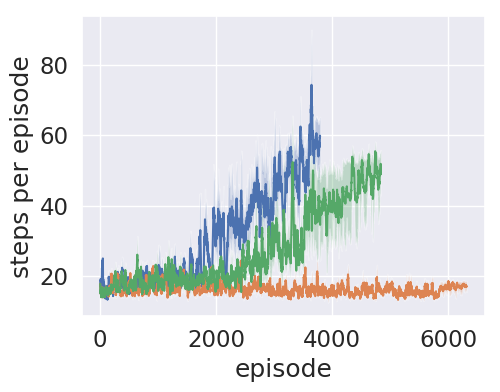
(b) CEM

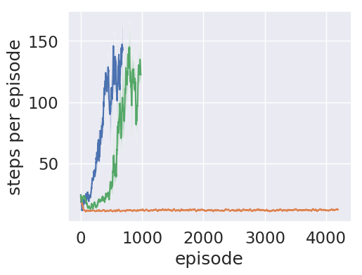
(c) SARSA

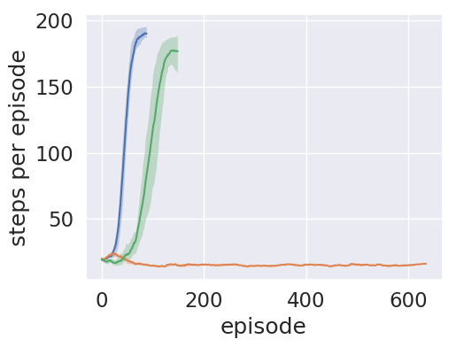
(d) DQN

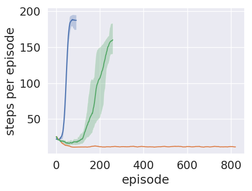
(e) Dueling-DQN

Figure 6: Complete learning curves from five reward robust RL algorithms (see Algorithm 3) on CartPole game with true rewards ($r$)  , noisy rewards ($\tilde{r}$) ($\eta=1$)   and estimated surrogate rewards ($\dot{r}$)  . Note that confusion matrices ${\mathbf{C}}$ are unknown to the agents here. From top to the bottom, the noise rates are 0.1, 0.3, 0.7 and 0.9. Here we repeated each experiment 10 times with different random seeds and plotted 10% to 90% percentile area with its mean highlighted.

$\omega=0.9$

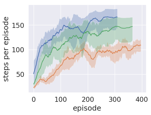
(a) $Q$-Learning

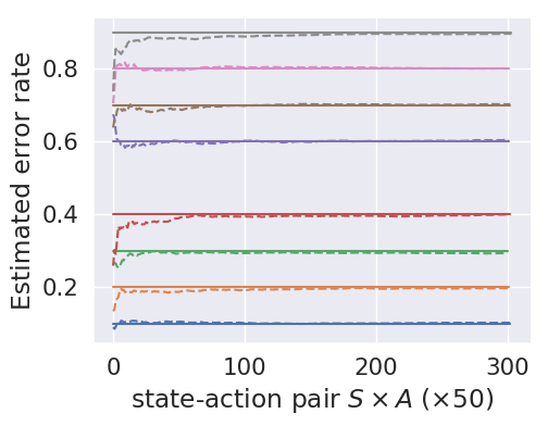
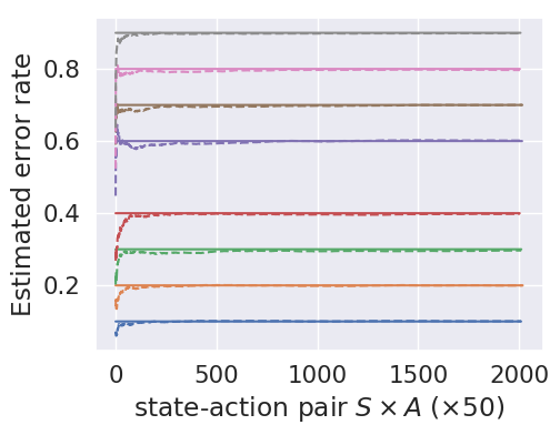
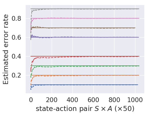
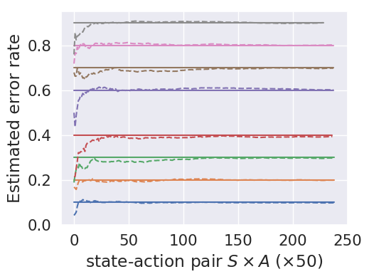
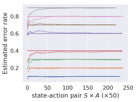
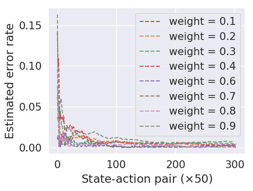
(a) $Q$-Learning

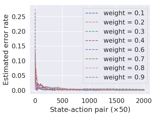
(b) CEM

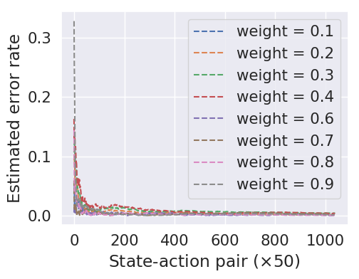
(c) SARSA

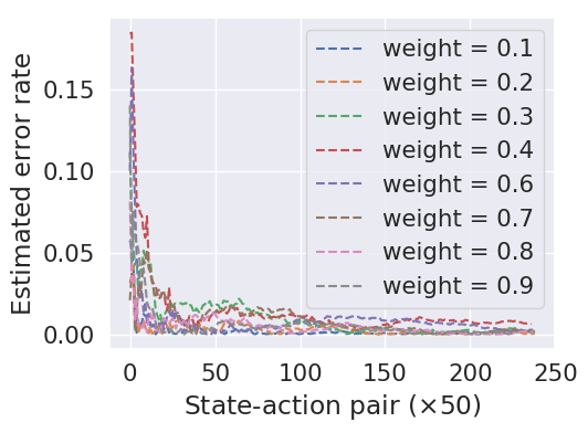
(d) DQN

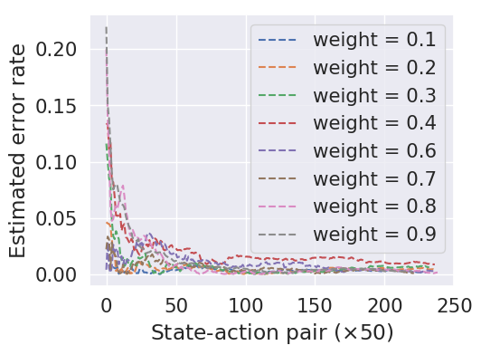
(e) Dueling-DQN

Figure 7: Estimation analysis from five reward robust RL algorithms (see Algorithm 3) on CartPole game. The upper figures are the convergence curves of estimated error rates (from 0.1 to 0.9), where the solid and dashed lines are ground truth and estimation, respectively; The lower figures are the absolute difference between the estimation and ground truth of confusion matrix ${\mathbf{C}}$ (normalized matrix norm).

$\omega=0.1$

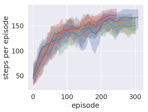
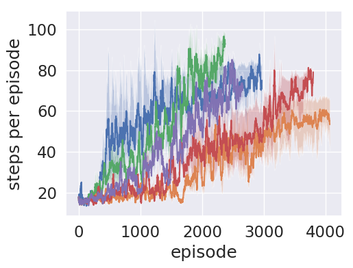
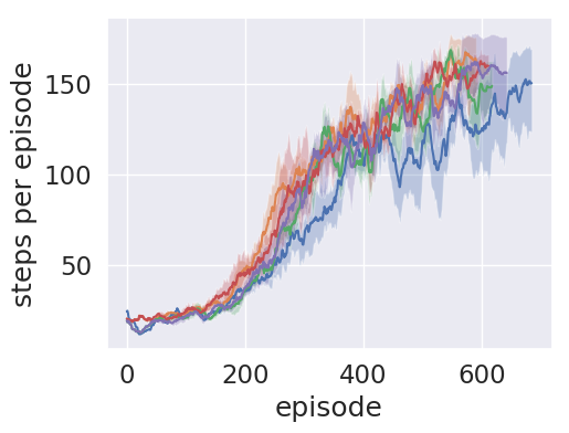
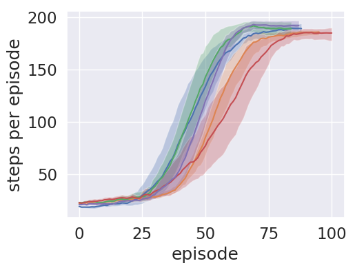
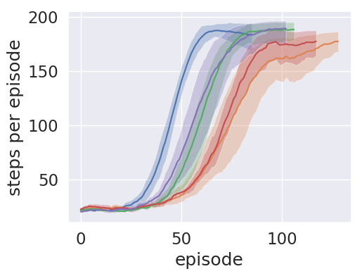
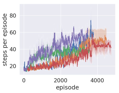
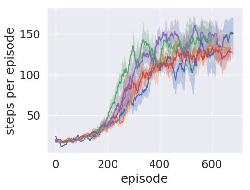
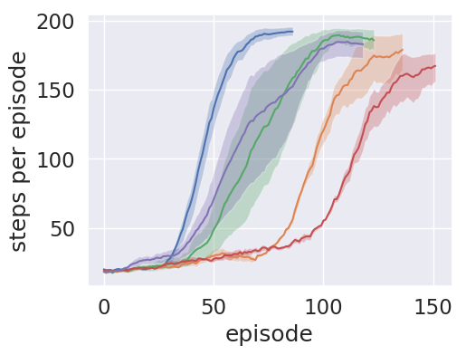
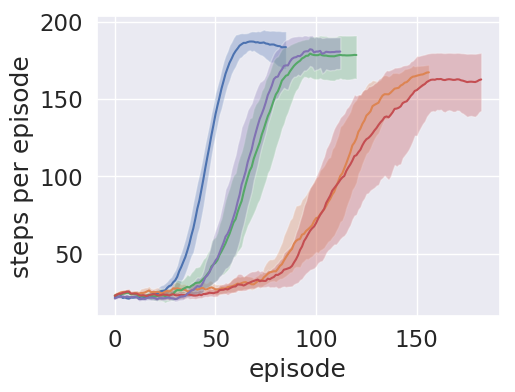
$\omega=0.3$

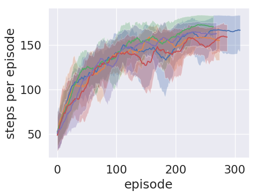
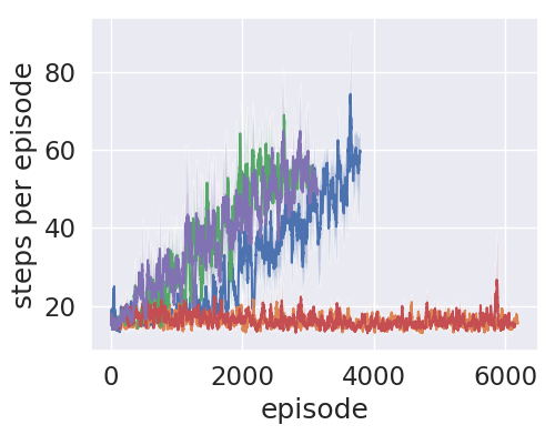
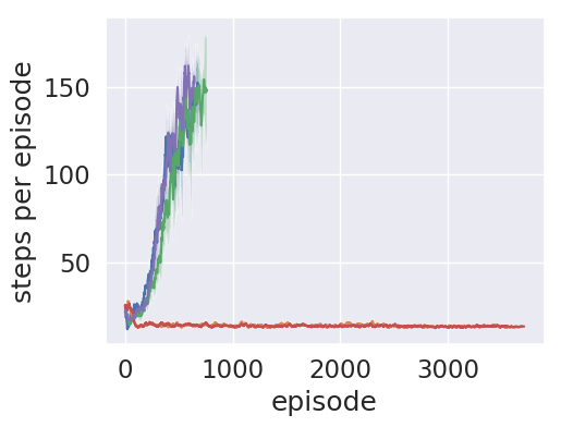
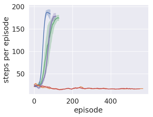
$\omega=0.7$

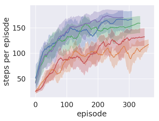
(b) CEM

(c) SARSA

(d) DQN

(e) DDQN

$\omega=0.9$

(a) $Q$-Learning

Figure 8: Learning curves from five reward robust RL algorithms (see Algorithm 3) on CartPole game with true rewards ($r$)  , noisy rewards ($\tilde{r}$) ($\eta=1$)  , sample-mean noisy rewards ($\eta=1$)  , estimated surrogate rewards ($\dot{r}$)   and sample-mean estimated surrogate rewards  . Note that confusion matrices ${\mathbf{C}}$ are unknown to the agents here. From top to the bottom, the noise rates are 0.1, 0.3, 0.7 and 0.9. Here we repeated each experiment 10 times with different random seeds and plotted 10% to 90% percentile area with its mean highlighted.

Table 4: Average scores of various RL algorithms on CartPole with sample-mean reward using variance reduction technique (VRT), surrogate rewards (ours) and the combination of them (ours + VRT). Note that the reward confusion matrices are unknown to the agents and each experiment is repeated three times with different random seeds.

Noise Rate	Reward	$Q$-Learn	CEM	SARSA	DQN	DDQN
$\omega=0.1$	VRT	173.5	99.7	167.3	181.9	187.4
	ours ($\dot{r}$)	181.9	99.3	171.5	200.0	185.6
	ours + VRT	184.5	98.2	174.2	199.3	186.5
$\omega=0.3$	VRT	140.4	43.9	149.8	182.7	177.6
	ours ($\dot{r}$)	161.1	81.8	159.6	186.7	200.0
	ours + VRT	161.6	82.2	159.8	188.4	198.2
$\omega=0.7$	VRT	71.1	16.1	13.2	15.6	14.7
	ours ($\dot{r}$)	172.1	83.0	174.4	189.3	191.3
	ours + VRT	182.3	79.5	178.9	195.9	194.2

Appendix D Supplementary Experimental Results

Visualizations on Control Games

$\omega=0.1$ $\omega=0.3$ $\omega=0.7$ $\omega=0.9$

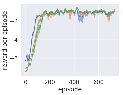
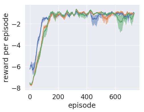
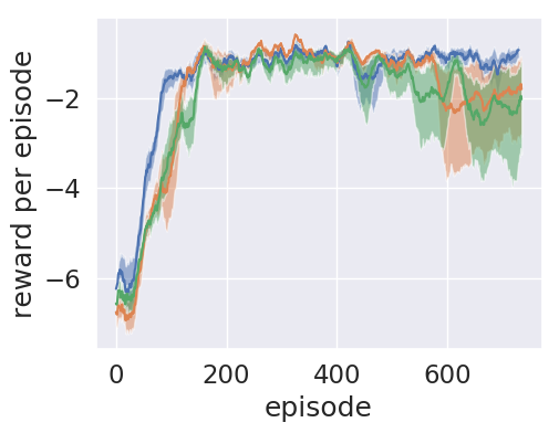
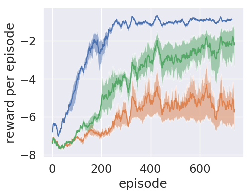
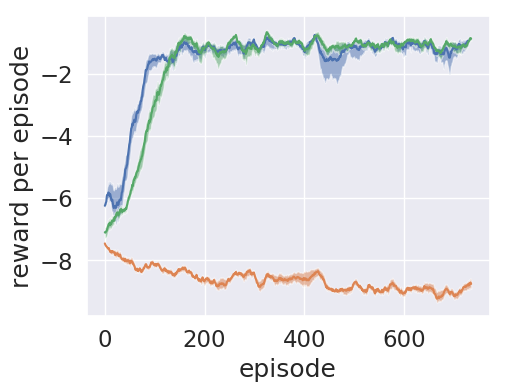
(a) DDPG (symmetric)

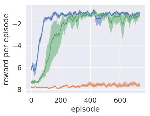
(b) DDPG (rand-one)

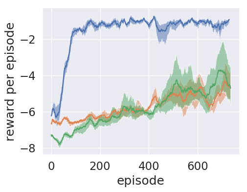
(c) DDPG (rand-all)

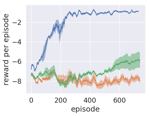
(d) NAF (rand-all)

Figure 9: Complete learning curves from DDPG and NAF on Pendulum game with true rewards ($r$)   , noisy rewards ($\tilde{r}$)   and surrogate rewards ($\hat{r}$) ($\eta=1$)  . Both symmetric and asymmetric noise are conduced in the experiments. From top to the bottom, the noise rates are 0.1, 0.3, 0.7 and 0.9, respectively. Here we repeated each experiment 6 times with different random seeds and plotted 10% to 90% percentile area with its mean highlighted.

Visualizations on Atari Games

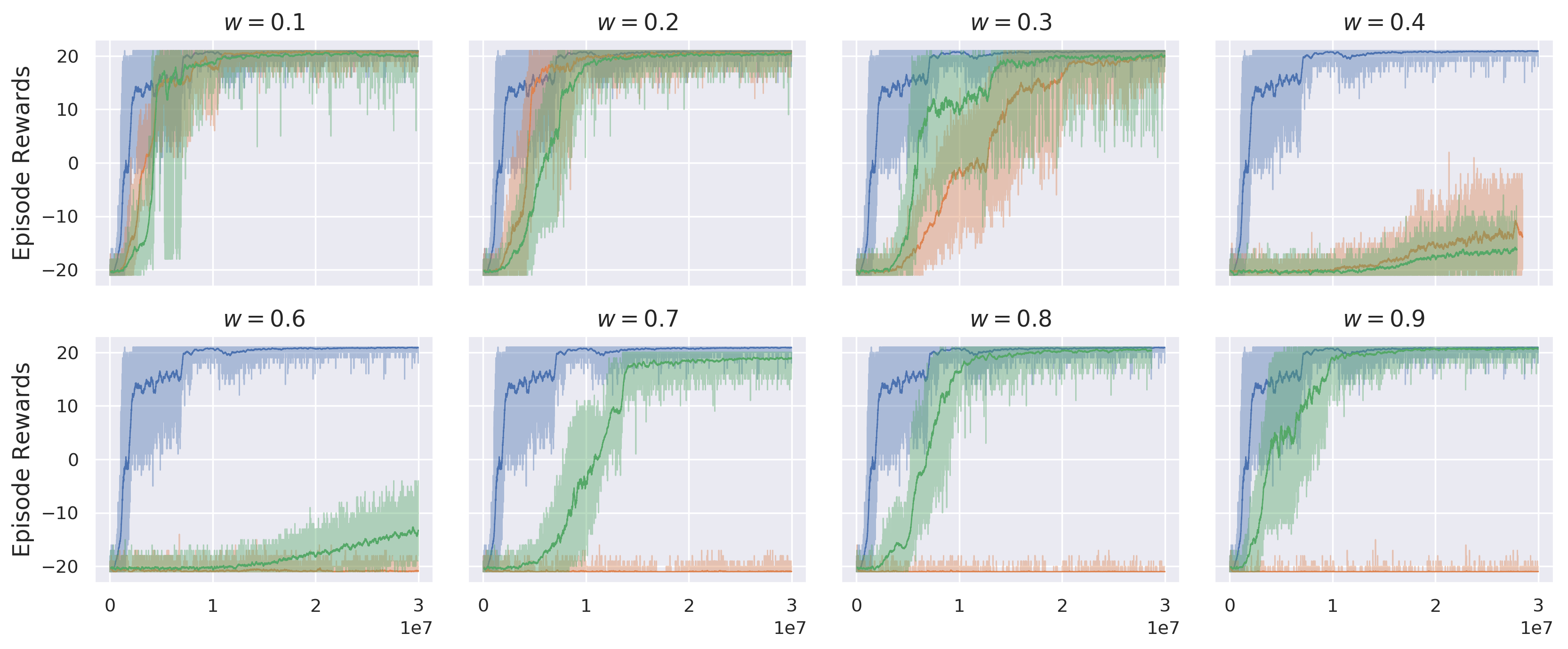
(a) Pong (sysmetric)

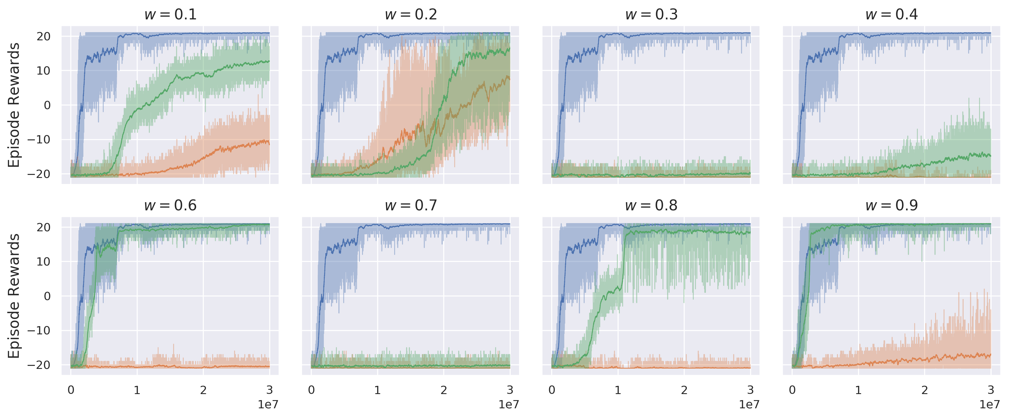
(b) Pong (rand-one)

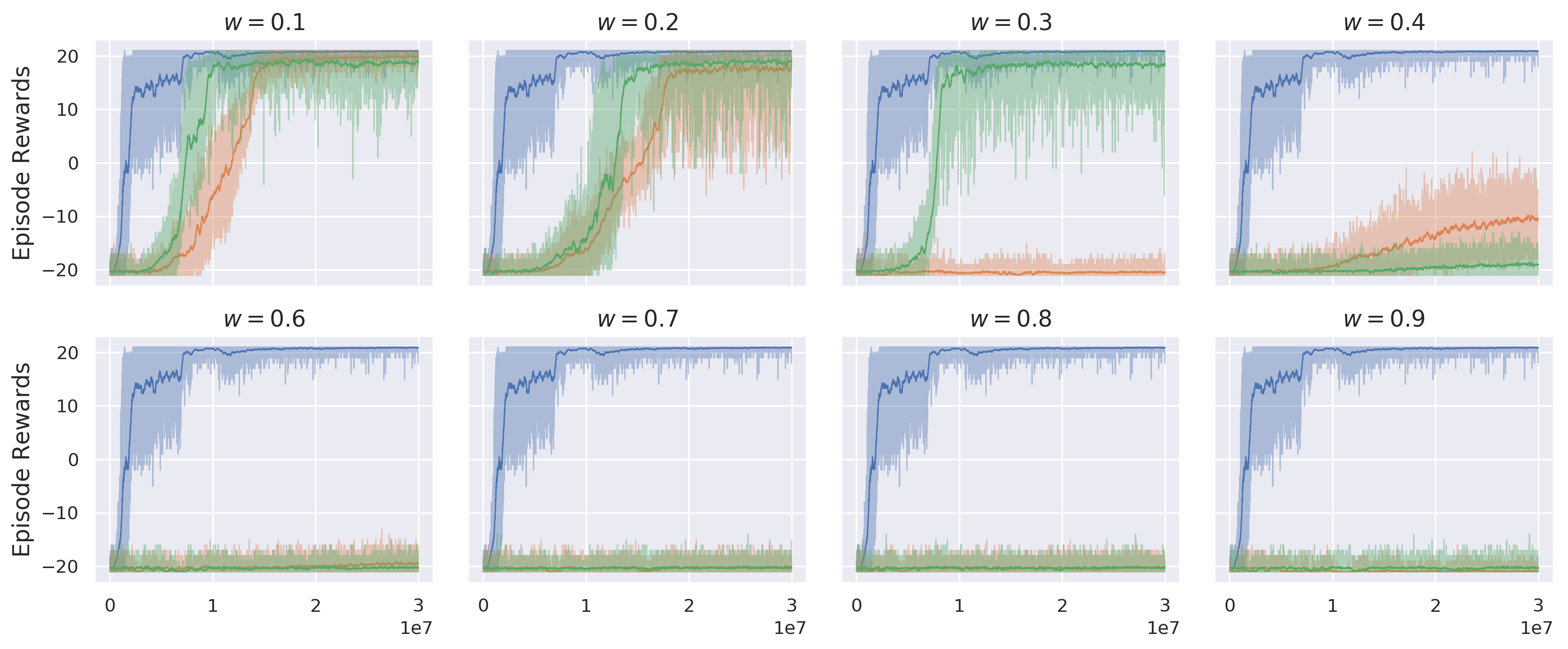
(c) Pong (rand-all)

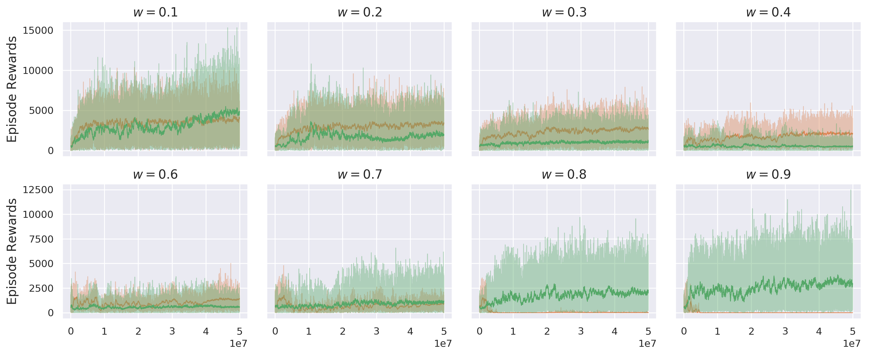
(a) AirRaid (sysmetric)

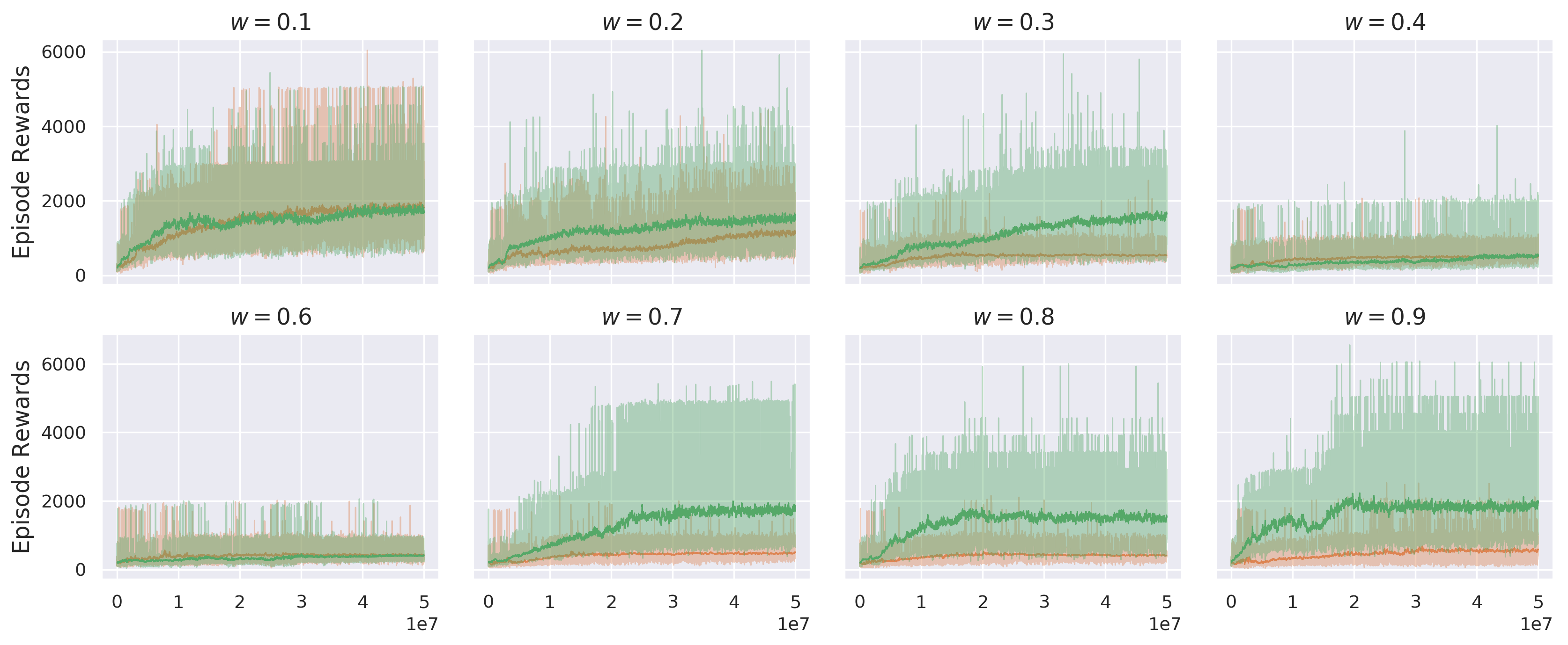
(b) Alien (sysmetric)

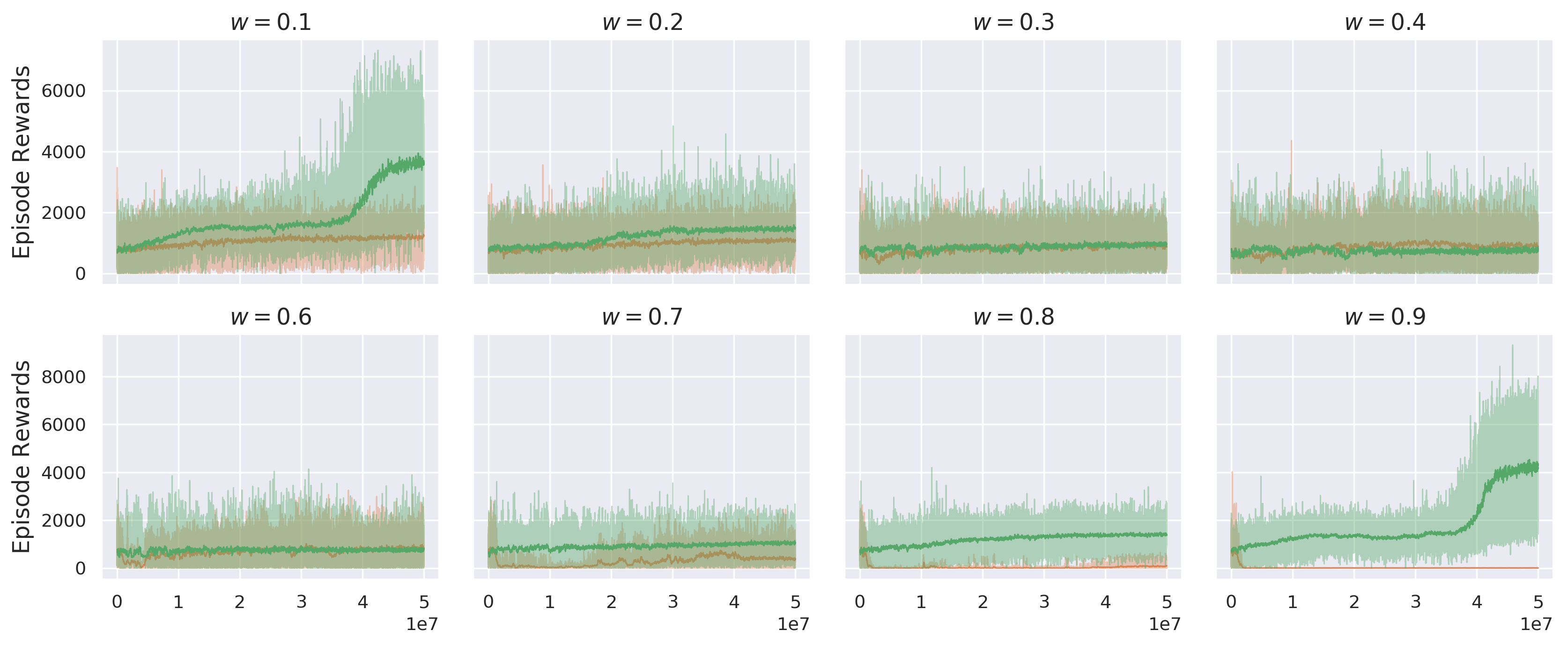
(c) Carnival (sysmetric)

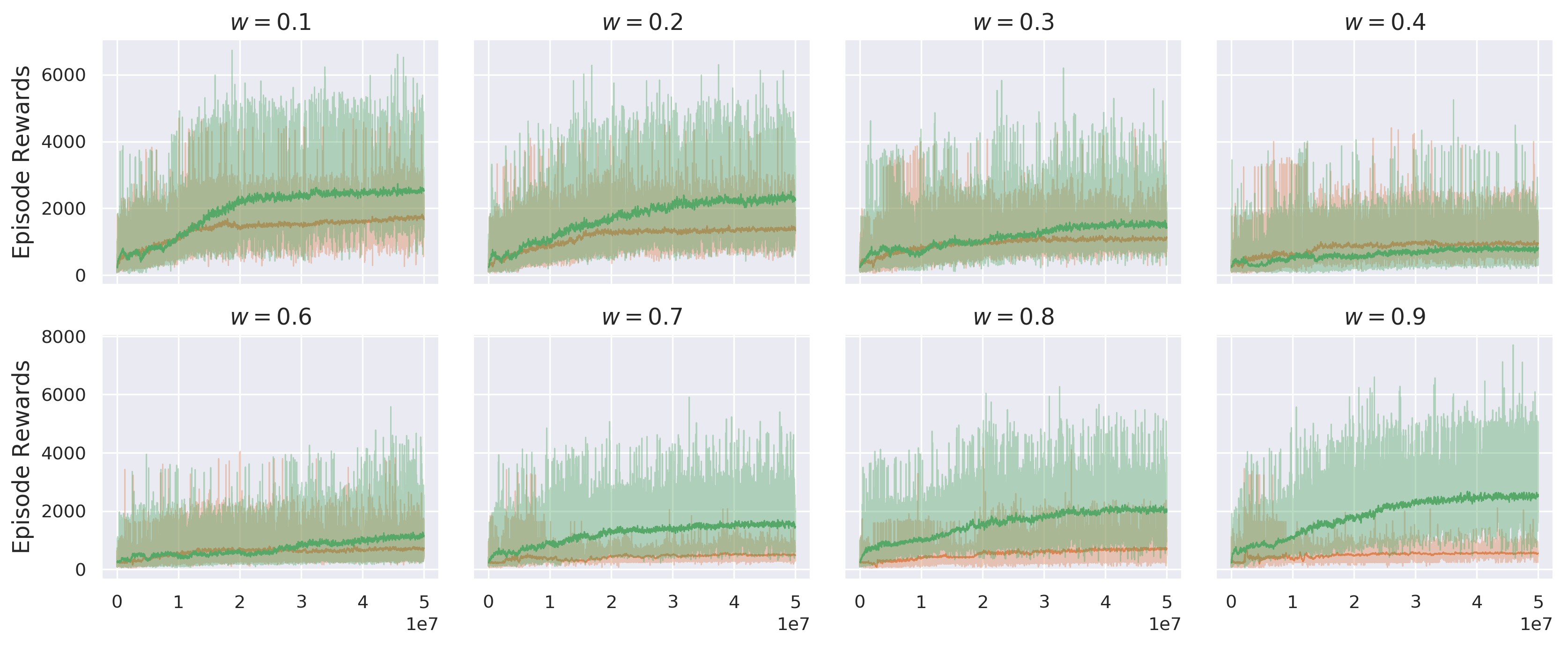
(a) MsPacman (sysmetric)

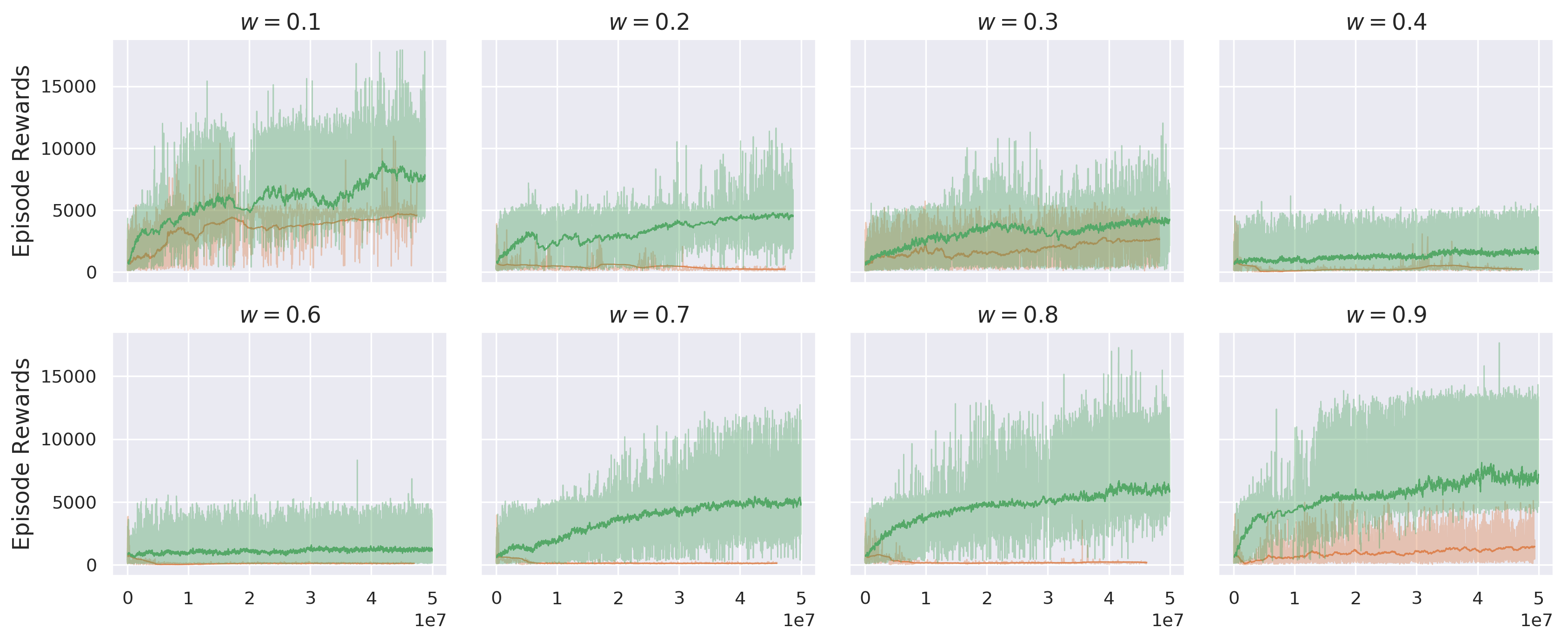
(b) Phoenix (sysmetric)

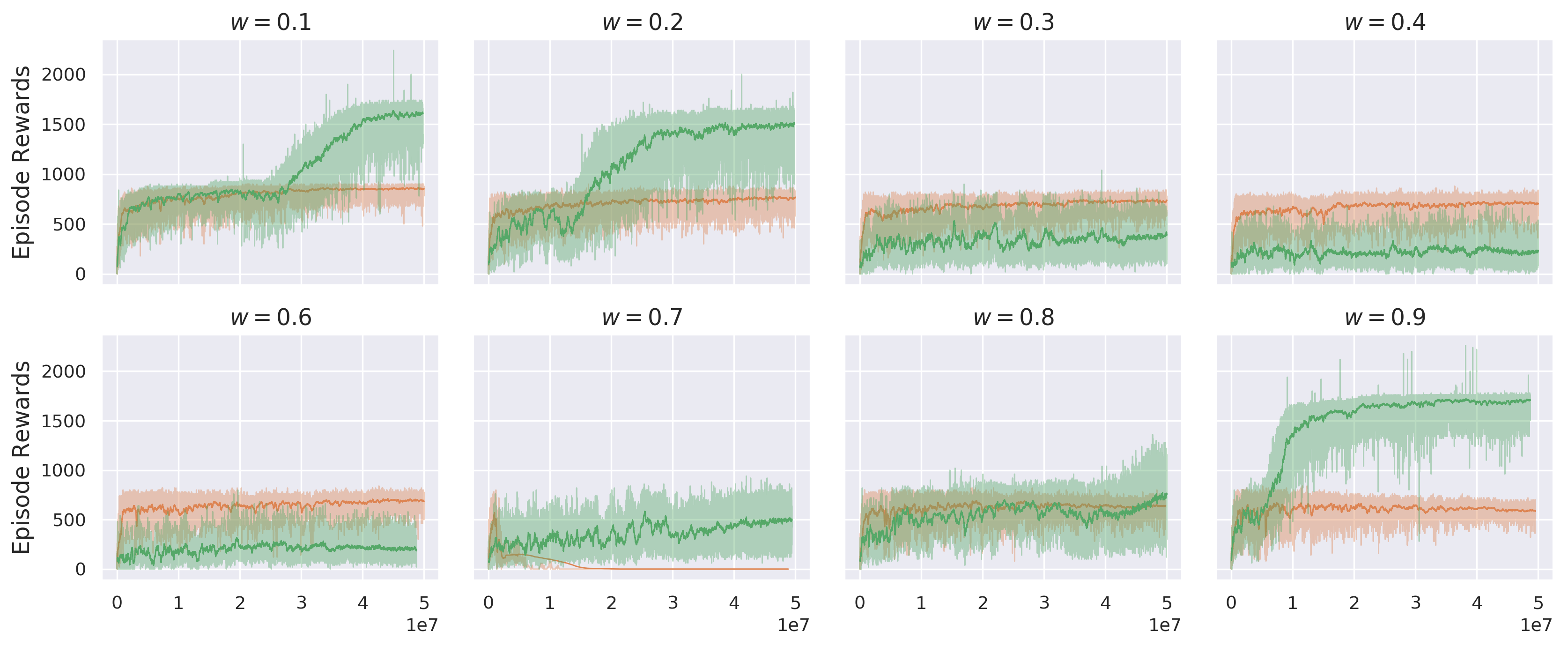
(c) Seaquest (sysmetric)

Figure 12: Complete learning curves from PPO on seven Atari game with true rewards ($r$)  , noisy rewards ($\tilde{r}$)   and surrogate rewards ($\eta=1$) ($\hat{r}$)  . The noise rates increase from 0.1 to 0.9, with a step of 0.1.

References

- [Bekker and Goldberger] Bekker, A. J., and Goldberger, J. 2016. Training deep neural-networks based on unreliable labels. In ICASSP, 2682–2686.
- [Brockman et al.] Brockman, G.; Cheung, V.; Pettersson, L.; Schneider, J.; Schulman, J.; Tang, J.; and Zaremba, W. 2016. Openai gym.
- [Dawid and Skene] Dawid, A. P., and Skene, A. M. 1979. Maximum likelihood estimation of observer error-rates using the em algorithm. Applied statistics 20–28.
- [Deisenroth, Rasmussen, and Fox] Deisenroth, M. P.; Rasmussen, C. E.; and Fox, D. 2011. Learning to control a low-cost manipulator using data-efficient reinforcement learning. In Robotics: Science and Systems.
- [Dhariwal et al.] Dhariwal, P.; Hesse, C.; Klimov, O.; Nichol, A.; Plappert, M.; Radford, A.; Schulman, J.; Sidor, S.; and Wu, Y. 2017. Openai baselines. https://github.com/openai/baselines.
- [Everitt et al.] Everitt, T.; Krakovna, V.; Orseau, L.; and Legg, S. 2017. Reinforcement learning with a corrupted reward channel. In IJCAI, 4705–4713.
- [Fu, Luo, and Levine] Fu, J.; Luo, K.; and Levine, S. 2017. Learning robust rewards with adversarial inverse reinforcement learning. CoRR abs/1710.11248.
- [Gu et al.] Gu, S.; Lillicrap, T. P.; Sutskever, I.; and Levine, S. 2016. Continuous deep q-learning with model-based acceleration. In ICML, volume 48, 2829–2838.
- [Gu, Jia, and Choset] Gu, Z.; Jia, Z.; and Choset, H. 2018. Adversary a3c for robust reinforcement learning.
- [Hadfield-Menell et al.] Hadfield-Menell, D.; Milli, S.; Abbeel, P.; Russell, S. J.; and Dragan, A. 2017. Inverse reward design. In NIPS, 6765–6774.
- [Hendrycks et al.] Hendrycks, D.; Mazeika, M.; Wilson, D.; and Gimpel, K. 2018. Using trusted data to train deep networks on labels corrupted by severe noise. CoRR abs/1802.05300.
- [Huang et al.] Huang, S.; Papernot, N.; Goodfellow, I.; Duan, Y.; and Abbeel, P. 2017. Adversarial attacks on neural network policies. arXiv preprint arXiv:1702.02284.
- [Irpan] Irpan, A. 2018. Deep reinforcement learning doesn’t work yet. https://www.alexirpan.com/2018/02/14/rl-hard.html.
- [Jaakkola, Jordan, and Singh] Jaakkola, T. S.; Jordan, M. I.; and Singh, S. P. 1993. Convergence of stochastic iterative dynamic programming algorithms. In NIPS, 703–710.
- [Kakade] Kakade, S. M. 2003. On the Sample Complexity of Reinforcement Learning. Ph.D. Dissertation, University of London.
- [Karger, Oh, and Shah] Karger, D. R.; Oh, S.; and Shah, D. 2011. Iterative learning for reliable crowdsourcing systems. In NIPS, 1953–1961.
- [Kearns and Singh] Kearns, M. J., and Singh, S. P. 1998. Finite-sample convergence rates for q-learning and indirect algorithms. In NIPS, 996–1002.
- [Kearns and Singh] Kearns, M. J., and Singh, S. P. 2000. Bias-variance error bounds for temporal difference updates. In COLT, 142–147.
- [Kearns, Mansour, and Ng] Kearns, M. J.; Mansour, Y.; and Ng, A. Y. 1999. A sparse sampling algorithm for near-optimal planning in large markov decision processes. In IJCAI, 1324–1231.
- [Khetan, Lipton, and Anandkumar] Khetan, A.; Lipton, Z. C.; and Anandkumar, A. 2017. Learning from noisy singly-labeled data. CoRR abs/1712.04577.
- [Kos and Song] Kos, J., and Song, D. 2017. Delving into adversarial attacks on deep policies. CoRR abs/1705.06452.
- [Lillicrap et al.] Lillicrap, T. P.; Hunt, J. J.; Pritzel, A.; Heess, N.; Erez, T.; Tassa, Y.; Silver, D.; and Wierstra, D. 2015. Continuous control with deep reinforcement learning. CoRR abs/1509.02971.
- [Lim, Xu, and Mannor] Lim, S. H.; Xu, H.; and Mannor, S. 2016. Reinforcement learning in robust markov decision processes. Math. Oper. Res. 41(4):1325–1353.
- [Lin et al.] Lin, Y.; Hong, Z.; Liao, Y.; Shih, M.; Liu, M.; and Sun, M. 2017. Tactics of adversarial attack on deep reinforcement learning agents. In IJCAI, 3756–3762.
- [Liu and Liu] Liu, Y., and Liu, M. 2017. An online learning approach to improving the quality of crowd-sourcing. IEEE/ACM Transactions on Networking 25(4):2166–2179.
- [Liu, Peng, and Ihler] Liu, Q.; Peng, J.; and Ihler, A. T. 2012. Variational inference for crowdsourcing. In NIPS, 701–709.
- [Loftin et al.] Loftin, R. T.; Peng, B.; MacGlashan, J.; Littman, M. L.; Taylor, M. E.; Huang, J.; and Roberts, D. L. 2014. Learning something from nothing: Leveraging implicit human feedback strategies. In RO-MAN, 607–612. IEEE.
- [Menon et al.] Menon, A.; Van Rooyen, B.; Ong, C. S.; and Williamson, B. 2015. Learning from corrupted binary labels via class-probability estimation. In ICML, 125–134.
- [Mnih et al.] Mnih, V.; Kavukcuoglu, K.; Silver, D.; Graves, A.; Antonoglou, I.; Wierstra, D.; and Riedmiller, M. A. 2013. Playing atari with deep reinforcement learning. CoRR abs/1312.5602.
- [Mnih et al.] Mnih, V.; Kavukcuoglu, K.; Silver, D.; Rusu, A. A.; Veness, J.; Bellemare, M. G.; Graves, A.; Riedmiller, M.; Fidjeland, A. K.; Ostrovski, G.; et al. 2015. Human-level control through deep reinforcement learning. Nature 518(7540):529.
- [Moreno et al.] Moreno, A.; Martín, J. D.; Soria, E.; Magdalena, R.; and Martínez, M. 2006. Noisy reinforcements in reinforcement learning: some case studies based on gridworlds. In WSEAS, 296–300.
- [Natarajan et al.] Natarajan, N.; Dhillon, I. S.; Ravikumar, P. K.; and Tewari, A. 2013. Learning with noisy labels. In Advances in neural information processing systems, 1196–1204.
- [Pendrith, Ryan, and others] Pendrith, M. D.; Ryan, M. R.; et al. 1997. Estimator variance in reinforcement learning: Theoretical problems and practical solutions.
- [Pinto et al.] Pinto, L.; Davidson, J.; Sukthankar, R.; and Gupta, A. 2017. Robust adversarial reinforcement learning. In ICML, volume 70, 2817–2826.
- [Plappert] Plappert, M. 2016. keras-rl. https://github.com/keras-rl/keras-rl.
- [Rajeswaran et al.] Rajeswaran, A.; Ghotra, S.; Levine, S.; and Ravindran, B. 2016. Epopt: Learning robust neural network policies using model ensembles. CoRR abs/1610.01283.
- [Romoff et al.] Romoff, J.; Piché, A.; Henderson, P.; François-Lavet, V.; and Pineau, J. 2018. Reward estimation for variance reduction in deep reinforcement learning. CoRR abs/1805.03359.
- [Roy, Xu, and Pokutta] Roy, A.; Xu, H.; and Pokutta, S. 2017. Reinforcement learning under model mismatch. CoRR abs/1706.04711.
- [Schulman et al.] Schulman, J.; Wolski, F.; Dhariwal, P.; Radford, A.; and Klimov, O. 2017. Proximal policy optimization algorithms. CoRR abs/1707.06347.
- [Schwartz] Schwartz, A. 1993. A reinforcement learning method for maximizing undiscounted rewards. In ICML, 298–305.
- [Scott et al.] Scott, C.; Blanchard, G.; Handy, G.; Pozzi, S.; and Flaska, M. 2013. Classification with asymmetric label noise: Consistency and maximal denoising. In COLT, 489–511.
- [Scott] Scott, C. 2015. A rate of convergence for mixture proportion estimation, with application to learning from noisy labels. In AISTATS.
- [Sobel] Sobel, M. J. 1994. Mean-variance tradeoffs in an undiscounted MDP. Operations Research 42(1):175–183.
- [Strens] Strens, M. J. A. 2000. A bayesian framework for reinforcement learning. In ICML, 943–950.
- [Sukhbaatar and Fergus] Sukhbaatar, S., and Fergus, R. 2014. Learning from noisy labels with deep neural networks. arXiv preprint arXiv:1406.2080 2(3):4.
- [Sutton and Barto] Sutton, R. S., and Barto, A. G. 1998. Reinforcement learning - an introduction. Adaptive computation and machine learning.
- [Szita and Lörincz] Szita, I., and Lörincz, A. 2006. Learning tetris using the noisy cross-entropy method. Neural Computation 18(12):2936–2941.
- [Teh et al.] Teh, Y. W.; Bapst, V.; Czarnecki, W. M.; Quan, J.; Kirkpatrick, J.; Hadsell, R.; Heess, N.; and Pascanu, R. 2017. Distral: Robust multitask reinforcement learning. In NIPS, 4499–4509.
- [Tsitsiklis] Tsitsiklis, J. N. 1994. Asynchronous stochastic approximation and q-learning. Machine Learning 16(3):185–202.
- [van Hasselt, Guez, and Silver] van Hasselt, H.; Guez, A.; and Silver, D. 2016. Deep reinforcement learning with double q-learning. In AAAI, 2094–2100.
- [van Rooyen and Williamson] van Rooyen, B., and Williamson, R. C. 2015. Learning in the presence of corruption. arXiv preprint arXiv:1504.00091.
- [Wang et al.] Wang, Z.; Schaul, T.; Hessel, M.; van Hasselt, H.; Lanctot, M.; and de Freitas, N. 2016. Dueling network architectures for deep reinforcement learning. In ICML, volume 48, 1995–2003.
- [Watkins and Dayan] Watkins, C. J. C. H., and Dayan, P. 1992. Q-learning. In Machine Learning, 279–292.
- [Watkins] Watkins, C. J. C. H. 1989. Learning from Delayed Rewards. Ph.D. Dissertation, King’s College, Cambridge, UK.