Extremely large telescopes
for complex stellar populations
around the Galactic centre

Abstract

The Galactic centre and its surrounding space are important in studying galaxy-scale evolution, and stellar populations therein are expected to have imprints of the long-term evolution. Interstellar extinction, however, severely limits optical observations, thereby requiring infrared observations. In addition, many systems from those in the proximity of the central black hole to foreground objects in the disc overlap in each sightline, which complicates the interpretation of observations of a wide variety of objects. We discuss some important issues concerning the central regions, particularly the Galactic bulge and the Nuclear Stellar Disc (also known as the Central Molecular Zone). An obvious advantage of Extremely Large Telescopes (ELTs) is the deeper limiting magnitudes, but we emphasise the importance of the synergy between the data of deep ELTs and other observational data (e.g.  astrometric measurements and the detection of interstellar absorption lines) in order to disentangle the complex stellar populations.

1 Introduction

The region within a few kiloparsecs from the Galactic centre (GC, hereinafter) is extremely interesting and complicated. In the very centre, a super massive black hole (BH) of a few million solar masses is surrounded by the Nuclear Stellar Cluster (NSC), which hosts stars—more than $10^{7}~{}{\rm M}_{\odot}$ within a few parsecs ([Genzel et al. (2010), Genzel et al. 2010]). Up to $\sim$250 pc around the centre is a disc system composed of stars, ${\sim}10^{9}~{}{\rm M}_{\odot}$, and interstellar gas (mainly molecular) and dust; the system is called the Nuclear Stellar Disc (NSD) and the Central Molecular Zone (CMZ) ([Morris & Serabyn (1996), Morris & Serabyn, 1996]; [Launhardt et al. (2002), Launhardt et al. 2002]). Around the NSD/CMZ and extended out to a few kiloparsecs is the Galactic bulge (GB), which is made up of a large number of stars, ${\sim}2\times 10^{10}~{}{\rm M}_{\odot}$ ([Valenti et al. (2016), Valenti et al. 2016]). Approximately at the Galactocentric distance of 3 kpc, the Galactic disc takes over as the main contributor to stellar populations in the Galactic disc. Generally speaking, observational studies on the innermost part of the disc are lacking, and the stellar populations around the interface between the GB and the disc remain elusive.

These regions, at around the distance of $\sim$8.3 kpc ([de Grijs & Bono (2016), de Grijs & Bono, 2016]), provide us with unique opportunities to investigate in detail the central components of a galaxy by observing individual stars and interstellar matter (ISM) down to a small scale. In fact, the last decade has seen many new results concerning stellar populations therein based on rapidly growing observational data from many large-scale, both photometric and spectroscopic, surveys targeting the GB (see the review by [Barbuy et al. (2018), Barbuy et al. 2018]). There are, however, a few difficulties in studying the central regions. First, strong interstellar extinction prevents us from observing the stars in shorter wavelengths and measuring their intrinsic brightness and colours. Dealing with the extinction towards the GC is especially hard, because it is patchy with respect to both the celestial position and the ling-of-sight (LoS) distance. Second, the interpretation of observational data is often complicated by the fact that various components of stars and ISM, including those in the foreground and background disc, are mixed along the LoS. In Section 2, we describe these problems as well as review some recent results and important unsolved issues. We then discuss some approaches in Section 3, which will become more and more practical by using data from Extremely Large Telescopes (ELTs) and other facilities. The high sensitivity of ELTs is a simple and clear advantage in observing faint stars (or stars of a given brightness with significantly shorter observational times and/or higher precision), as we present in Section 4, but combining various types of data is crucial for disentangling the mixed stellar populations around the GC.

2 Recent progress and unsolved matters

2.1 Nuclear Stellar Cluster (NSC)

With intensive and sustained efforts, many publications on the NSC have been reported in the literature. The results based on near-infrared data cover a broad range including the mass of the central BH, the distance to the GC based on stellar orbits around Sgr A^∗, and stellar populations within the cluster ([Genzel et al. (2010), Genzel et al. 2010]; [Fritz et al. (2016), Fritz et al. 2016], and references therein). Detailed observations of stars and ISM in the proximity of the central BH allow us to investigate exciting events, which are useful for testing fundamental processes in astronomy and physics ([Plewa et al. (2017), Plewa et al. 2017]; [GRAVITY Collaboration (2018), GRAVITY Collaboration, 2018]). This cluster is also unique among stellar clusters in the Galaxy because it hosts stellar populations with a wide range of ages from a few megayears to older than 5 Gyr ([Pfuhl et al. (2011), Pfuhl et al. 2011]; see also a report of RR Lyrae in [Dong et al. (2017), Dong et al. 2017]). A long-standing issue is the formation and growth of the NSC and the presence of young stars (e.g.  [Antonini (2013), Antonini, 2013]; [Lu et al. (2014), Lu et al. 2014]; [Yelda et al. (2014), Yelda et al. 2014]); are they formed in situ, and if so where does the ISM come from and how can it lose its angular momentum and fall into the central part? The most likely source for such ISM is the gas of the CMZ, but the mechanism(s) of the gas transfer is/are unclear ([Gallego & Cuadra (2017), Gallego & Cuadra, 2017]). Although the main focus of this contribution is on the NSD/CMZ and the GB, and not on the NSC, studying the evolution of ISM and stars in the NSD/CMZ is relevant to important questions about the NSC and the related evolution of the Galaxy. For example, the circulation of ISM among these systems may be important for the growth of the central BH and the BH–host coevolution ([Kormendy & Ho (2013), Kormendy & Ho, 2013]).

2.2 Nuclear Stellar Disc/Central Molecular Zone (NSD/CMZ)

The presence of the high-density disc-like system has been recognised for a long time, since early infrared and radio observations ([Blitz et al. (1993), Blitz et al.  1993]; [Morris & Serabyn (1996), Morris & Serabyn, 1996]), and the overall and basic properties of the NSD/CMZ were summarised by [Launhardt et al. (2002)]. This relatively small region harbours 3–10 % of the total molecular gas and star formation of the Galaxy ([Kauffmann (2017), Kauffmann, 2017]). There exist various types of stars of a wide range of ages, including young stars such as blue luminous variables and Wolf–Rayet stars (especially those in the Arches and Quintuplet clusters aged at $\sim$4 Myr; [Stolte et al. (2014), Stolte et al. 2014], and references therein) and a few classical Cepheids aged $\sim$25 Myr (Matsunaga et al. [Matsunaga et al. (2011), 2011], [Matsunaga et al. (2015), 2015]). Besides, the observations of ISM, mainly in radio wavelengths, have been very active ([Morris & Serabyn (1996), Morris & Serabyn, 1996]; [Kauffmann et al. (2017), Kauffmann et al. 2017]). Here, we raise two questions concerning star formation and stellar ages in the NSD/CMZ.

How to supply gas for the episodic star formation in the NSD/CMZ.
The star formation rate in the NSD/CMZ in the past few megayears has been estimated at ${\sim}0.1~{}M_{\odot}\,{\rm yr}^{-1}$ ([Barnes et al. (2017), Barnes et al. 2017]). The ISM must be supplied from somewhere outside to explain the stellar mass (${\sim}10^{9}~{}M_{\odot}$) as well as the ISM mass (${\sim}10^{7}~{}M_{\odot}$) in the NSD/CMZ ([Launhardt et al. (2002), Launhardt et al. 2002]). One plausible path of the gas transfer is the highly elongated orbits along the bar structure through which the ISM in the inner disc can fall to the CMZ ([Binney et al. (1991), Binney et al. 1991]; [Kim et al. (2011), Kim et al. 2011]; [Sormani et al. (2015), Sormani et al. 2015]). Moreover, it has been suggested that the star formation in the NSD/CMZ is episodic, with a time scale of order 20 Myr ([Stark et al.  (2004), Stark et al. 2004]; [Krumholz & Kruijssen (2015), Krumholz & Kruijssen, 2015]; [Krumholz et al.  (2017), Krumholz et al. 2017]). In fact, based on the period distribution of Cepheids in the NSD, [Matsunaga et al. (2011)] concluded that the star formation rate 30–70 Myr ago was lower than the rate 20–30 Myr ago. In addition to the three classical Cepheids at $\sim$25 Myr found in the original survey, [Matsunaga et al. (2015)] found a new classical Cepheid which is very similar in age and other properties to the three, and also considered to be within the NSD. Together, the four Cepheids indicate a star formation rate of $0.1^{+0.2}_{-0.05}~{}{\rm M}_{\odot}\,{\rm yr}^{-1}$ in 20–30 Myr ago, which is higher than the rate in 30–70 Myr ($<0.02~{}{\rm M}_{\odot}\,{\rm yr}^{-1}$, as inferred from the absence of Cepheids with such ages). To better understand the physical conditions of the star formation in the NSD/CMZ, the distribution and substructures of the ISM and young stars within this region is important. It has been long known that the distribution of the CMZ ISM is highly asymmetric in Galactic longitude and radial velocity, $v_{\rm LoS}$ ([Bally et al. (1988), Bally et al. 1988]). However, it is difficult to know the LoS positions of the ISM, as well as those of stars within the NSD/CMZ. The information on $v_{\rm LoS}$ is useful; [Molinari et al. (2011)], for example, discovered an outstanding $\infty$-shaped feature, in projection, of dust and combined the dust map with $v_{\rm LoS}$ data of CS molecules to infer the twisted elliptical ring (see also [Kruijssen et al. (2015), Kruijssen et al. 2015]). With many components mixed along the LoS, however, ambiguity tends to remain in such analysis. Whereas an overall distribution characterised by a ring (not a pan cake) structure has been seen in many studies, recent studies suggest that various substructures such as small spiral arms ([Sofue (1995), Sofue, 1995]; [Sawada et al. (2004), Sawada et al. 2004]) and streams ([Kruijssen et al. (2015), Kruijssen et al. 2015]) can be naturally produced in hydrodynamical simulations of barred galaxies, where the gas transfer from the bar to the central part is also predicted (Sormani et al. [Sormani et al. (2015), 2015], [Sormani et al. (2018), 2018]; [Ridley et al. (2017), Ridley et al. 2017]). Detailed mappings of the ISM and stellar populations making use of astrometric data, which give proper motions, and interstellar absorption features would be useful to verify the distribution of the ISM. Moreover, knowing the locations and kinematics of stars, especially young stars, within the NSD/CMZ is also crucial for understanding the evolution of this system.

Oldest stars in the NSD/CMZ and the formation of the system.
Whereas the NSD/CMZ clearly hosts young stars as mentioned above, the age of the oldest stars therein is unclear. Because many old stars exist in the GB, it is necessary to identify stars in the NSD/CMZ based on kinematics. A group of evolved AGB stars with maser emission, in particular OH/IR stars, are known to show a concentration towards the NSD/CMZ and kinematics consistent with its disc rotation ([Lindqvist et al. (1992), Lindqvist et al. 1992]; [Deguchi et al. (2004), Deguchi et al. 2004]). The ages of these objects are not clear, but are considered to be intermediate, say 0.1–5 Gyr. SiO masers, at the GC distance, are mostly detected in Miras with period longer than $\sim$400 days ([Deguchi et al. (2004), Deguchi et al. 2004]), which are supposedly younger than those in globular clusters that have $P\lesssim 300$ days (see, e.g. [Catchpole et al. (2016), Catchpole et al. 2016], concerning ages and periods of Miras in the bulge). In contrast, RR Lyrae and type II Cepheids, if found in the NSD/CMZ, would be conclusive tracers of an old population. However, they are rather faint owing to the strong extinction, $2\lesssim A_{K}\lesssim 3$ (e.g.  see Fig. 1 in [Contreras Ramos et al. (2018), Contreras Ramos et al. 2018]), especially when we need to know their kinematics to distinguish them from the GB population. [Dong et al. (2017)] reported the discovery of RR Lyrae in the NSC using deep HST/WFC3 images, but the oldest stars in the NSD/CMZ are not necessarily coeval with the counterparts in the NSC. [Matsunaga et al. (2013)] suggested the presence of old stars in the NSD/CMZ based on the excess of short-period ($<350$ days) Miras and type II Cepheids over the density gradient of these objects in the GB, but this result is indirect and also needs to be confirmed with more complete samples of these variable stars. Thus, the oldest stars in the NSD/CMZ remain to be identified. It would also be sensible to ask if the first stars of the system were formed therein or accumulated through a dynamical process. This may be related to another question, ‘when did the bar form?’, if we accept the gas transfer through the bar as the ISM fuelling mechanism for the CMZ and that the first stars were formed in situ. To answer these questions, deeper surveys of variable stars and the kinematic identification of the NSD/CMZ members will be useful.

2.3 Galactic bulge (GB)

Whereas optical observations are prohibitive for the above two components, the NSC and NSD/CMZ, owing to high extinction ($A_{V}\gtrsim 30$ mag), the GB can be observed in the optical regime, at least at longer wavelengths. This has allowed many large-scale surveys in the optical, together with those in the infrared, to produce massive datasets which have triggered rapid growth in our knowledge, especially in the recent decades (see, e.g.  the contribution by Valenti in this volume). In the low-latitude regions, however, optical observations are very limited, and strong extinction at $|b|\lesssim 1^{\circ}$ causes serious problems, even in the near infrared, as we see in Section 2.4.

The GB has an elongated structure, although stars with different ages may be distributed differently, and kinematics and chemical abundances of stars show systematic trends depending on the position (see, e.g.  [Ness & Freeman (2016), Ness & Freeman, 2016]; [Portail et al. (2017), Portail et al. 2017]; [Zoccali et al. (2017), Zoccali et al. 2017]). Whereas the GB itself can be called a bar with its elongated structure, other bars, longer and thinner than the GB, have been suggested, although the situation is not so clear (see reviews by [Bland-Hawthorn & Gerhard (2016), Bland-Hawthorn & Gerhard, 2016], and [Zoccali & Valenti (2016), Zoccali & Valenti, 2016]). It is predicted that orbits along the bar structure produce cold and high-$v_{\rm LoS}$ features and such orbits may be preferentially occupied by young bar stars, age $\lesssim$2–3 Gyr ([Aumer & Schönrich (2015), Aumer & Schönrich, 2015]). OH/IR stars and SiO maser sources show kinematics expected for the bar-like orbits ([Habing (2016), Habing, 2016]), while high velocity components seen in APOGEE’s data may also be following the expected bar kinematics ([Palicio et al. (2018), Palicio et al. 2018], and references therein). Among many new findings regarding the GB based on various large-scale surveys ([Barbuy et al. (2018), Barbuy et al. 2018]), in the following discussions, we focus on two important issues concerned with stellar populations in the GB: namely, the presence of intermediate-age stars and the X-shaped structure, both of which remain to be fully confirmed.

Intermediate-age stars in the GB.
Canonical results mainly based on photometric data suggest that the bulge is composed almost purely of old stars, $\gtrsim 10$ Gyr ([Kuijken & Rich (2002), Kuijken & Rich, 2002]; [Zoccali et al. (2003), Zoccali et al. 2003]; [Clarkson et al. (2011), Clarckson et al. 2011]). In contrast, Bensby et al. ([Bensby et al. (2013), 2013], [Bensby et al. (2017), 2017]) obtained high-resolution spectra of microlensed dwarfs and subgiants and, in the 2017 paper, they concluded that more than 35 % of metal-rich stars, [Fe/H]$>0$, are younger than 8 Gyr. [Bensby et al. (2017)] also found that such younger stars show hot kinematics like older GB stars. The presence of the intermediate-age stars was supported by [Bernard et al. (2018)], who used an intensive dataset collected by HST/WFC3 and concluded that 20–25 % of metal-rich stars (or 10 % of the bulge stars) are younger than 5 Gyr. However, using similar or even larger datasets, [Clarkson et al. (2011)] and [Renzini et al. (2018)] found no evidence of a significant population of young ($\lesssim 5$ Gyr) stars. It has been suggested that old stellar populations with enhanced helium abundance may resolve such a conflict, although an anomalously high helium enrichment seems to be required ([Nataf & Gould (2012), Nataf & Gould, 2012]; [Nataf (2016), Nataf, 2016]; [Renzini et al. (2018), Renzini et al. 2018]). Some types of bright evolved stars may contribute to this issue if one can give accurate ages for those in the last evolutionary phases with short time scales. For example, mass-losing AGB stars with maser emission ([Blommaert et al. (2018), Blommaert et al. 2018]; [Trapp et al. (2018), Trapp et al. 2018]) and carbon-rich stars ([Matsunaga et al. (2017), Matsunaga et al. 2017]) often indicate intermediate-age populations. However, the methods of determining the ages of such objects have not been fully established. Moreover, short evolutionary phases are expected to give a relatively small number of objects, and the interpretation of such rare objects requires caution considering the presence of blue star stragglers ([Clarkson et al. (2011), Clarkson et al. 2011]), which are old but may mimic objects evolved from heavier single stars.

Double red clump and the X shape of the GB.
Using large-scale 2MASS and/or OGLE data, [McWilliam & Zoccali (2010)] and [Nataf et al.  (2010)] detected two split peaks of the red clump (or a double RC) at high Galactic latitudes, $|b|\gtrsim 5^{\circ}$, in the GB. Many studies have concluded that this feature reflects the X shape that characterises a peanut-shaped bulge ([Zoccali & Valenti (2016), Zoccali & Valenti, 2016], and references therein). Some works claim that the double RC can be explained by the presence of helium-enhanced populations (Lee et al. [Lee et al. (2015), 2015], [Lee et al. (2018), 2018]). There are increasing publications concerning the double RC and the X shape of the GB (e.g. [Ness et al. (2012), Ness et al. 2012]; [Wegg & Gerhard (2013), Wegg & Gerhard, 2013]; [Gonzalez et al. (2015), Gonzalez et al. 2015]; [Ness & Lang (2016), Ness & Lang, 2016]; López-Corredoira, [López Corredoira (2016), 2016], [López Corredoira (2017), 2017]; [Joo et al. (2017), Joo et al. 2017]). See also the point raised by E. Valenti, which is given in the Discussion section of this contribution. It is worthwhile to note at least that different stellar populations have different distributions. For example, the old (and probably metal-poor) population represented by RR Lyrae, type II Cepheids, and short-period Miras do not show evidence of the X-shaped structure ([Pietrukowicz et al. (2013), Pietrukowicz et al. 2013]; [Catchpole et al. (2016), Catchpole et al. 2016]; [Bhardwaj et al. (2017), Bhardwaj et al. 2017]; [Braga et al. (2018), Braga et al. 2018]). It is therefore important to understand the parameters (age, metallicity, and helium abundance if possible; see Section 3.4) of stars being investigated.

2.4 Extinction towards the GC

It is well known that regions towards the GC are severely obscured by interstellar extinction, and observations of stars therein are limited or complicated by its effects. For example, the Optical Gravitational Lensing Experiment (OGLE) has discovered over 38,000 RR Lyrae in a large area towards the GB, but very few were found within $\sim$1.5 degrees of the Galactic plane ([Soszyński et al. (2014), Soszynski et al. 2014]). More recently, Gaia Data Release 2 (DR2) compiled the first catalogue from the all-sky variability search ([Gaia Collaboration (2018b), Gaia Collaboration, 2018b]; [Holl et al. (2018), Holl et al. 2018]), and [Mowlavi et al.  (2018)], studying long-period variables, found that the low-latitude region ($|b|\lesssim 1^{\circ}$) is the zone of avoidance (see their Fig. 46). According to the extinction map of [Dutra et al. (2003)], the extinction at $\sim$2 $\mu$m, $A_{K}$, gets higher than 1 mag in such a low-latitude region. Infrared observations are much less affected, but there are still challenging issues. Strong extinction tends to render stars such as RR Lyrae, which are not so luminous intrinsically, below detection limits of surveys ([Contreras Ramos et al. (2018), Contreras Ramos et al. 2018]). Once reddened objects are detected, it is crucial to accurately know the extinction law, i.e.  the wavelength dependency of the extinction, to discuss the distribution of stellar populations in highly obscured regions such as the inner Galaxy (see the reviews of [Matsunaga (2017), Matsunaga, 2017], and [Matsunaga et al. (2018), Matsunaga et al.  2018]).

It is important to keep in mind that the extinction towards the GC is very patchy. For example, [Matsunaga et al. (2009)] estimated the reddenings and extinctions of short-period ($<350$ days) Miras within ${\sim}0.3^{\circ}$ around the GC. In their study, although $\sim$150 Miras with distance and $A_{K}$ obtained are projected towards the NSD/CMZ and most of them are located at almost the same distance, 8.24 kpc, the precision of individual distances is not high enough to determine whether the Miras belong to the NSD/CMZ or to the GB. The derived extinctions range from $\sim$2 mag to more than 3.5 mag and vary with the celestial position within a small angular distance; in some cases, two Miras separated by only a couple of arc-minutes have $A_{K}$ different by more than 1 mag (see Fig. 25 in [Matsunaga et al. (2009), Matsunaga et al. 2009]). Whereas foreground molecular clouds clearly cause the patchy extinction pattern, resulting in some regions being free of any Miras found at the bulge distance, part of the large scatter in $A_{K}$ may be attributed to the dust within the NSD/CMZ. It is possible that stars in its front are less reddened compared to those on the far side, although distances to individual objects are not precise enough to confirm such a systematic effect. There are a few three-dimensional extinction maps which give the extinction as a function of the celestial coordinate and distance, and that by [Schultheis et al. (2014)], who used VVV and 2MASS data, is particularly useful for the regions around the GC. The authors found that a large amount of dust exists in front of the Galactic bar, at 5–7 kpc, but the resolution was insufficient to discuss the extinction within or near the NSD/CMZ (or the data were not deep enough). Nevertheless, a couple of studies have suggested a significant amount of extinction within the NSD ([Launhardt et al. (2002), Launhardt et al. 2002]; [Oka et al. (2005), Oka et al. 2005]). For the NSC, [Chatzopoulos et al. (2015b)] performed a detailed study on the kinematics of stars that seems to be skewed owing to the selection bias caused by the additional extinction, and concluded that the dust within the NSC is responsible for $\sim$15 %, $A_{K}\simeq 0.4$ mag, of the total extinction. They demonstrated that the distribution and kinematics of stars can provide information on the distribution of the absorbing ISM (see also Section 3.1).

3 Approaches for disentangling mixed populations in the GC

In order to address the issues we discussed in Section 2, there are certain observational challenges. An obvious advantage of ELTs is the deeper limiting magnitudes, but it will be important to combine the deep ELT data with various kinds of other observational data when we confront the challenges, as discussed below. First, when observed objects are located in the LoS with many overlapping components, e.g.  the NSD, GB, and foreground/background disc, it is necessary to know which system individual objects belong to. Furthermore, it would be useful to locate the objects inside the system in question. It has been, however, very hard to determine locations within the NSD with the radius of $\sim$250 pc (0.07 mag in distance modulus), e.g.  by taking the correction of the severe extinction into account. Astrometric data leading to three-dimensional velocities when combined with radial velocities would allow us to locate stars, at least roughly, within the NSD (Section 3.1). In addition, the detection of absorption features caused by the ISM would provide valuable information on the locations of both stars and the intervening ISM (Section 3.2). This latter approach can also help us deal with the second challenge: we need to estimate the foreground extinction for each object because of the very patchy nature of the extinction towards the GC (Section 3.2). The third challenge lies in carrying out spectroscopic measurements of faint dwarfs and subgiants in the GB as much as possible, for which the ELTs’ high sensitivity is of direct importance, and we will also discuss the merits of microlensing surveys in the infrared in Section 3.3. Finally, for both topics raised for the GB (Section 2.3), helium abundance may play a key role in understanding the important characteristics of the relevant stellar populations. It would be of great value if we could measure the helium abundances of stars in the GB, and we will discuss the possibility of direct measurements using a helium line in the near infrared in Section 3.4, although it is not entirely clear how easily and accurately the abundances can be measured.

3.1 Astrometric data

A common problem in understanding objects in the NSD is, as mentioned above, that the precision of distances to them is usually not high enough to determine where along the LoS, e.g.  on which of the near and far sides, they are located, even if one could identify objects belonging to the NSD. It is usually impossible to reduce the distance errors to $\pm 250$ pc at the distance of $\sim$8.3 kpc (i.e.  3 %), taking into account the uncertainty in the foreground extinction and other errors. Additionally, such a precision (3.5 $\mu$as in parallax) is very difficult to achieve, which will likely be the case even for future astrometric observations (either infrared or radio wavelengths). Radial velocities, $v_{\rm LoS}$, leave an ambiguity between near and far distances, even if we consider circular orbits only. To overcome this problem, proper motions are expected to be very useful. Precise proper motions, especially those in the $b$ direction, allow us to clean a sample of stars in the NSD/CMZ ($\mu_{b}\sim 0$), which is otherwise severely contaminated by stars in the GB with a large velocity dispersion, $\sigma(\mu_{b})\gtrsim 3$ mas yr^-1 ([Soto et al. (2014), Soto et al. 2014]). A precision of $\sim$0.3 mas yr^-1 is desirable for selecting the NSD/CMZ stars efficiently. In contrast, proper motions in the $l$ direction, $\mu_{l*}$, would enable us to locate stars inside the NSD/CMZ, because stars on the near side and those on the far side are expected to have opposite tangential velocities owing to the rotation within the NSD/CMZ. For example, [Chatzopoulos et al. (2015b)] made use of $\mu_{l*}$ as a proxy of the far–near positions of stars inside the NSC, following a similar idea but based on a sophisticated model of the cluster, and estimated the extinction caused by dust within the NSC. Similar approaches can be used for the NSD/CMZ stars when the necessary astrometric data become available. Considerable uncertainties can remain in the locations of the stars, considering the possibility of open orbits, but it is possible to distinguish the near and far distances as long as we assume that the objects are not counter-rotating in the NSD/CMZ ([Stolte et al. (2014), Stolte et al. 2014]; [Kruijssen et al. (2015), Kruijssen et al. 2015]). The use of $v_{\rm LoS}$ and $\mu_{l*}$ is also discussed in detail by [Debattista et al. (2018)]. In particular, their Figure 3 shows predicted trends of the velocities as functions of the position around the GC for two groups with different ages and different kinematics (one dominated by stars streaming along the bar and the other for those in the nuclear disc).

Long-term monitoring surveys from the ground allow us to measure the proper motions of stars even though the precision is not so high as that of astrometric satellites. As an early achievement, [Sumi et al. (2003)] detected the streaming motion of the Galactic bar by measuring the proper motions of red clump giants based on four-season, 1997–2000, data from OGLE-II. The precision of the proper motion was typically 1–2 mas yr^-1 for individual stars ([Sumi et al. (2004), Sumi et al. 2004]), and using thousands of stars allowed the detection of the tangential streaming motion of $\sim$1.6 mas yr^-1, corresponding to $\sim$100 km s^-1 (see also follow-up studies by [McWilliam & Zoccali (2010), McWilliam & Zoccali, 2010], and [Poleski et al. (2013), Poleski et al. 2013]). Recently, [Smith et al. (2018)] compiled a catalogue of astrometric measurements based on VVV survey data, and they obtained proper motions with statistical uncertainties below 1 mas yr^-1 for nearly 50 million stars. These measurements are useful to study the kinematics of stars around the GC, although the precision is not very high for individual stars. Similar or higher precision can be achieved with AO-applied images (e.g.  [Stolte et al. (2014), Stolte et al. 2014]) with a smaller number of epochs, but such observations cover smaller fields-of-view than the large-scale surveys mentioned above. Compared to ground-based measurements, space projects with astrometric satellites have a clear advantage in terms of the precision. Gaia has been providing very precise measurements of proper motions, in addition to parallaxes, with the median error of 50 $\mu$as yr^-1 in the DR2 for a large number of stars in the Galaxy ([Gaia Collaboration (2018a), Gaia Collaboration, 2018a]; [Lindegren et al. (2018), Lindegren et al. 2018]), and the errors will be smaller than 10 $\mu$as yr^-1 for sufficiently bright stars at the end of mission. However, its observation in the optical wavelengths cannot reach the inner regions of the Galaxy. There are a few plans which can give space-borne astrometric measurements in the infrared, namely Small-JASMINE ([Gouda (2018), Gouda, 2018]), WFIRST ([WFIRST Astrometry Working Group (2017), WFIRST Astrometry Working Group, 2017]), and GaiaNIR ([Hobbs et al. (2016), Hobbs et al. 2016]). At the distance of 8 kpc, the precisions of $\sim$0.5 mas yr^-1 (ground-based) and $\lesssim 25$ $\mu$as yr^-1 (Small-JASMINE) correspond to the tangential velocities of 20 and 1 km s^-1, respectively. As for Small-JASMINE, in addition to bright main objects (approximately 7,000 bulge stars with $H_{\rm W}<12.5$) for which the precision of 25 $\mu$as yr^-1 or higher is targeted, there is a plan to observe fainter objects ($\sim$70,000 bulge stars with $H_{\rm W}<15$) with lower precision $\sim$125 $\mu$as yr^-1. This intermediate precision, which corresponds to 5 km s^-1 at the GC distance, will be useful for filling the gap between the objects with the best proper motions and those with ground-based astrometry.

3.2 Interstellar absorption features

Interstellar clouds not only attenuate signals to be accounted for (broad-)band magnitudes, but also imprint absorption features in stellar spectra. Such absorptions reflect the amount of extinction and the velocity structure of the absorbing materials. Here, we here discuss diffuse interstellar bands (DIBs) and absorption lines by certain molecules that have been observed in stars, particularly those in the direction of the GC.

DIBs can be useful to determine foreground extinctions of individual objects. Some DIBs in the optical wavelengths have been found to show good correlation between their equivalent widths (EWs) and the extinction (e.g.  [Kashuba et al. (2016), Kashuba et al. 2016]). In contrast, at least some other lines show the so-called skin effect which gives scatters around simple reddening–EW(DIB) relations depending on the atomic/molecular ratio along intervening clouds ([Herbig (1995), Herbig, 1995]; [Lan et al. (2015), Lan et al. 2015]). In any case, the ranges of the extinction investigated by using optical DIBs are limited, compared to the extinction towards the GC regions, in previous studies. [Damineli et al. (2017)] extended the relationship between the 8,620 Å DIB and the extinction up to $A_{K}\sim 0.8$ mag by observing stars in the famous massive cluster Westerlund 1 in the inner Galaxy ($l=-20.5^{\circ},b=-0.4^{\circ}$). This particular DIB feature will be especially important, because it is included within the wavelength range of Gaia’s radial velocity spectrometer (RVS). For severely reddened stars in the innermost part of the Galaxy, it is necessary to identify DIBs in the infrared range showing good correlations with the extinction. For example, [Cox et al. (2014)] detected more than 20 DIBs in the wide range of the NIR, 0.9–2.5 $\mu$m, observed with the VLT/X-Shooter, including 11 candidate DIBs they newly identified. Later, Hamano et al. ([Hamano et al. (2015), 2015], [Hamano et al. (2016), 2016]) found nearly 20 DIBs at 0.98–1.32 $\mu$m with WINERED spectra ($R\sim 28,000$), and [Galazutdinov et al. (2017)] detected 14 DIBs at 1.46–2.40 $\mu$m with IGRINS spectra ($R\sim 45,000$). Both spectrographs used for these works can produce high-quality spectra (S/N$\gtrsim 500$), which is important for the detection of many shallow DIBs, down to $\sim$5 mÅ with WINERED or $\sim$30 mÅ with IGRINS. We can expect that DIBs in severely reddened stars are relatively stronger, and in fact [Geballe et al. (2011)] detected 13 DIBs in a few objects located within the NSD/CMZ at 1.5–1.8 $\mu$m in the $H$ band only. Nevertheless, it is important to obtain high-resolution and high-quality spectra especially if one would like to know the velocity profile of the DIB absorption. A comprehensive review of DIBs is found in [Krelowski (2018)], which mainly discusses the optical DIBs but also includes the infrared ones.

The relations between the DIBs’ EWs and the extinction, once established, can be used to estimate the extinctions of individual objects. Such estimates would be independent of the distances of objects and work as an alternative or complementary method to photometry-based methods. Furthermore, DIBs can provide valuable information on the velocity distribution of absorbing ISM. For example, DIBs produced by the ISM in the NSD/CMZ are characterised by a large velocity dispersion, $\sim$150 km s^-1 ([Geballe et al. (2011), Geballe et al. 2011]), in contrast to most of the foreground ISM which has almost zero velocity in the direction of the GC. Recently, making use of the large dataset of the APOGEE, [Zasowski et al.  (2015)] found that the DIB with $\lambda_{0}=$15,273 Å, according to their determination, shows red- (or blue-) shifts following the Galactic rotation (see also Elyajouri et al. [Elyajouri et al.  (2016), 2016], [Elyajouri et al.  (2017), 2017], for DIBs in APOGEE spectra). It should be noted that the FWHMs of DIBs tend to be large compared to those of lines of interstellar atoms and molecules, which we discuss below. In addition, the profile of the band and even the central wavelength may be subject to the physical conditions of the absorbing ISM ([Cami et al. (2004), Cami et al. 2004]; [Oka et al. (2013), Oka et al. 2013]). These can blur and/or bias the velocity distribution inferred from DIBs.

Different types of absorption features caused by ISM are also useful. For example, the absorption lines of ${\rm H}_{3}^{+}$ in the $L$ band have been intensively investigated with the spectra of early-type stars located around the GC ([Goto et al. (2002), Goto et al. 2002]; [Oka et al. (2005), Oka et al. 2005], and references therein). The advantage of these lines is their sharpness, which makes it possible to identify velocity components with high resolution as demonstrated in the above works. Furthermore, the ${\rm H}_{3}^{+}$ absorptions in different transitions enable us to investigate the physical and chemical conditions of the ISM in the NSD/CMZ and elsewhere ([Goto et al. (2014), Goto et al. 2014]; [Le Petit et al. (2016), Le Petit et al. 2016]). Other useful features for studying interstellar absorption include the lines of CO and the less-investigated H₂ (e.g.  Goto et al. [Goto et al. (2014), 2014], [Goto et al. (2015), 2015]; [Lacy et al. (2017), Lacy et al. 2017]) in the $K$ band, and combining these features would allow further detailed investigations of the chemical status of the ISM.

The interstellar features discussed here are rather weak in most cases, and it is crucial to collect high-quality spectra (i.e.  high resolution and high S/N). Whereas some features are detectable with the resolution of $\sim$20,000, e.g.  the DIB studied with the APOGEE, higher resolving power ($R\gtrsim 50,000$) is desirable considering the sharpness of the interstellar absorption lines. Their strengths do not exceed 10 % in depth, even in the spectra of stars at around the GC, thus requiring high S/N of a few hundred. DIBs in the spectra of cool stars ([Monreal-Ibero & Lallement (2017), Monreal-Ibero & Lallement, 2017]) may be very useful for studying the ISM towards the GC regions, but there are a few issues: large errors in the databases of stellar lines in the IR, and diversity of the objects in temperature and chemical abundances. Relative spectral analyses comparing stars in the NSD/CMZ and the inner GB with those which have similar parameters but significantly weaker DIBs in the outer GB may make it easier to measure the DIB components. After all, the GC regions are full of cool stars, and it will be possible to find very similar stars. Studying DIBs in Cepheids is also interesting, especially those located in the disc, considering that individual Cepheids give good estimates of distance and reddening thanks to the period–luminosity and period–colour relations ([Kashuba et al. (2016), Kashuba et al. 2016]), although the task may be even more challenging owing to the pulsation causing spectral variation of each Cepheid (e.g.  offsets and asymmetric profiles of lines).

3.3 Spectroscopy for bulge dwarfs/subgiants with and without microlensing events

As described in Section 2.3, an important question about the age distribution of stellar populations in the GB came with high-resolution spectroscopic observations of microlensed dwarfs and subgiants ([Bensby et al. (2013), Bensby et al. 2013]). They are too faint for current high-resolution spectrographs with 8-m class telescopes, but the microlensing events with amplitudes of 10–2,000 sufficiently brightened the targets. The high sensitivity of ELTs will enable us to observe dwarfs and subgiants in the GB even without the microlensing events as we evaluate in Section 4.

Most of the previously detected microlensing events are limited by the sensitivity of optical microlensing surveys, and they are away from the Galactic plane by 1.5 degrees or more. In contrast, a pioneering survey using UKIRT successfully detected microlensing events at low Galactic latitudes, $-0.98\leq b\leq-0.36$ degrees ([Shvartzvald et al. (2017), Shvartzvald et al. 2017]). [Navarro et al. (2017)] further reported nearly 200 microlensing events detected in the VVV survey for five years in $\sim$5 deg² around the GC. A great jump in infrared microlensing surveys will be delivered by the WFIRST project being planned for the mid-2020s ([Bennett et al. (2018), Bennett et al. 2018]). There are also plans for ground-based microlensing surveys in the infrared including PRIME (a new 1.3-m telescope with a 1.3-deg² wide-field camera being constructed in South Africa) in addition to the currently active infrared facilities, UKIRT and VISTA ([Yee et al. (2018), Yee et al. 2018]). Such surveys in the future will allow us to study dwarfs and subgiants in the low-latitude regions by using the same technique as [Bensby et al. (2013)] and other studies, but based on infrared photometric and spectroscopic observations.

3.4 He I 10,830 Å and helium abundance

Despite its importance in stellar structure and evolution, measurements of helium abundance using helium line(s) have not been performed particularly intensively. Direct measurements of helium abundance are not so easy, as we discuss below. Readers are also referred to valuable reviews in [Gratton et al.  (2012)] and [Bastian & Lardo (2018)]. There are some methods for indirectly measuring the helium abundances of stellar populations based on photometric data, e.g.  the so-called $R$ parameter ([Iben (1968), Iben, 1968]; [Salaris et al. (2004), Salaris et al. 2004]) and the properties of RR Lyrae ([Marconi & Minniti (2018), Marconi & Minniti, 2018]; [Marconi et al. (2018), Marconi et al. 2018]), but the direct measurements are of great value for investigating the mixed populations in the GC regions.

In shorter optical wavelengths ($<5,900$ Å), some photospheric He I lines can be detected, but they appear only in hot stars ($\gtrsim 9,000$ K). Such hot stars in old stellar populations appear during the horizontal branch (HB) phase, but radiative levitation or gravitational settling of various elements can occur in the turbulence-free atmosphere of sufficiently hot HB stars ([Grundahl et al.  (1999), Grundahl et al. 1999]; [Behr et al. (1999), Behr et al. 1999]; [Behr (2003), Behr, 2003]). This process produces the $u$ jump observed in colour–magnitude diagrams: the hotter stars appear distinctly bright in the Strömgren $u$ band ([Grundahl et al.  (1999), Grundahl et al. 1999]). Fortunately, for HB stars in the narrow temperature range of $9,000\lesssim T_{\rm eff}\lesssim 11,500$ K, the He abundance can be measured without the diffusion depletion, and such measurements have been reported for several globular clusters using the photospheric He I line at 5875 Å ([Gratton et al.  (2014), Gratton et al. 2014]; [Mucciarelli et al.  (2014), Mucciarelli et al. 2014], and references therein). The temperature of the $u$ jump (or the Grundahl jump) has been found to be $\sim$ 11,500 K for most globular clusters, but it can also vary with the helium abundance as suggested by [Tailo et al. (2017)]. Unfortunately, these photospheric He I lines in the optical regime are of limited use for stars in the GC regions. First, the hot HB stars are faint at ${\sim}$8 kpc for high-resolution spectroscopy, and the interstellar extinction makes necessary optical observations prohibitive, except for low-extinction regions of the outer bulge. Second, with the high metallicity of the bulge stars, HB is no longer extended to the hot temperature range.

The He I 10,830 Å line exists in the near-infrared range, and this line is observable in FGK giants (Dupree et al. [Dupree et al. (1992), 1992], [Dupree et al. (2009), 2009]). It has been used in several studies on the helium abundances of multiple populations in globular clusters ([Dupree et al. (2011), Dupree et al. 2011]; [Pasquini et al. (2011), Pasquini et al. 2011]; [Dupree & Avrett (2013), Dupree & Avrett, 2013]; [Smith et al. (2014), Smith et al. 2014]; [Strader et al. (2015), Strader et al. 2015]). An important point which should be kept in mind about this line is, however, that it is formed in stellar chromospheres, and the abundances cannot be obtained without careful, challenging modelling of the chromosphere ([Strader et al. (2015), Strader et al. 2015]). In addition to many other scientific targets (e.g.  [Izotov et al. (2014), Izotov et al. 2014]; [Aver et al. (2015), Aver et al. 2015]; [Spake et al. (2018), Spake et al. 2018]), this line can be used for a variety of applications, such as the dynamics in the envelopes of different types of objects, e.g.  the Sun ([Dupree et al. (2005), Dupree et al. 2005]), metal-poor giants ([Dupree et al. (2009), Dupree et al. 2009]), metal-poor dwarfs ([Takeda & Takada-Hidai (2011), Takeda & Takada-Hidai, 2011]), active stars ([Sanz-Forcada & Deupree (2008), Sanz-Forcada & Dupree, 2008]; [Fuhrmeister et al. (2018), Fuhrmeister et al. 2018]), and young stellar objects ([Takami et al. (2002), Takami et al. 2002]; [Connelley & Greene (2010), Connelley & Greene, 2010]; [Reipurth et al. (2010), Reipurth et al. 2010]; [Cauley & Johns-Krull (2014), Cauley & Johns-Krull, 2014]). Combined, these applications provide strong motivation to establish the usage of the He I 10,830 Å in general and the chromosphere models in particular for predicting the formation of this line.

It should be noted that, apart from the theoretical challenge of modelling the chromosphere, there are certain observational challenges in investigating the He I 10,830 Å line of red giants in the GC regions. First, there are a few telluric absorption lines around this wavelength (see, e.g.  [Sameshima et al. (2018), Sameshima et al. 2018]), and they should be accurately removed. Second, ThAr lamps, which are most often used for wavelength calibration, do not show many lines around the wavelength ([Kerber et al. (2008), Kerber et al. 2008]); a low-accuracy dispersion solution can cause a problem, especially if the He line is weak and blended with a telluric line. A practical approach is to use late-type giants with established radial velocity as wavelength standards (e.g.  [Dupree et al. (2011), Dupree et al. 2011]), but new calibration sources under development, e.g.  lamps with other elements such as uranium ([Redman et al. (2011), Redman et al. 2011]) and laser frequency combs ([Osterman et al. (2012), Osterman et al. 2012]), will eventually enable accurate and robust calibration. Third, the He I line is expected to be weak or invisible in the main bulk of bright red giants in the bulge. It gets strongest, $\gtrsim 300$ mÅ, at the spectral types of G and early K, and becomes weaker, $\lesssim$100 mÅ at 5,000 K or lower, as effective temperature decreases ([Vaughan & Zirin (1968), Vaughan & Zirin, 1968]; [Strader et al. (2015), Strader et al. 2015]). Therefore, we need to collect high-resolution spectra of early-K giants (or those with even earlier spectral type) or late-K giants with extremely high S/N. The effective temperature of red clump giants is approximately 5,000 K, which indicates that the main targets have $J<15$ even in the lowest-extinction regions of the GB. This is roughly the limit of the current good spectrographs attached to 8-m class telescopes, considering the required high quality, but ELTs will reach such targets, as we discuss in Section 4.

4 Observational opportunities with ELTs

In this section, we briefly discuss what types of tracers in different regions around the GC can be reached with the expected limiting magnitudes of ELTs. We focus on high-resolution near-infrared spectroscopy ($R\equiv\lambda/\Delta\lambda\gtrsim 20,000$). According to [Zieleniewski et al.  (2015)], for example, HARMONI attached to E-ELT is expected to reach approximately $J=19.5$ and $K=19.5$, in the Vega magnitude scale, for $R=20,000$ with S/N$=$50 for five hours on-source. We use these limits as a guideline in the following discussion. It is crucial to collect high-quality (high-resolution and high-S/N) spectra for many science targets discussed in this contribution. In particular, studying DIBs and lines of interstellar molecules requires S/N as high as a few hundred, as mentioned in Section 3.2, and the limiting magnitudes for the relevant projects would probably be $\sim$2 mag shallower. Such a high requirement means that the high photon-collecting powers of ELTs will be higly advantageous once suitable high-resolution spectrographs are installed. High-quality spectroscopy will be also important for measuring the abundances of extremely metal-poor stars in the bulge (see, e.g.  Howes et al.  [Howes et al. (2015), 2015], [Howes et al. (2016), 2016]), once such candidates are identified, although the necessary quality for such projects is less demanding than the interstellar absorption features.

Figure 1 plots isochrones offset by the distance modulus of the GC, $14.6$ mag, as well as by different reddenings and extinctions ($A_{K}=0.5,1.5$, and 2.5 mag), following the reddening vector of [Nishiyama et al. (2006)]. The isochrones for 10 Gyr (solid curve) and 100 Myr (dashed curve), both with solar metallicity, are taken from the MESA Isochrones & Stellar Tracks (MIST) website ([Choi et al. (2016), Choi et al. 2016]), and the evolutionary phases prior to thermal-pulsing AGB are included. Upper main-sequence stars of young stellar populations are good targets for highly precise detection of interstellar absorption features in the $K$ band and longer wavelengths, even in the heavily obscured regions, $A_{K}\gtrsim 3$ mag (Section 3.2). The typical positions of the red clump at different extinctions ($A_{K}=0,1,2$, and 3 mag) are also indicated by squares connected by the line whose slope corresponds to that of the reddening vector. Comparing the two panels clearly shows that objects quickly get faint in $J$ more than in $K$ with increasing extinction. For example, the RC in the NSD/CMZ is not available for high-resolution spectroscopy in $J$ but observable in $K$.

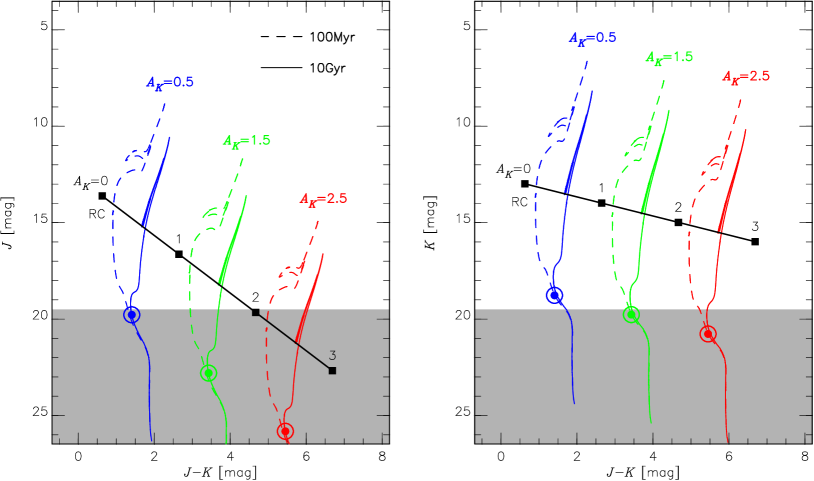
Figure 1: Isochrones shifted down to the distance of the GC ($\mu_{0}=14.6$ mag) but with different reddenings and extinctions, $A_{K}$, added as indicated in the colour–magnitude diagram: $(J-K)$–$J$ (left) and $(J-K)$–$K$ (right). The selected extinctions, $A_{K}=0.5,1.5$, and 2.5 mag, correspond to the typical values for the high-latitude GB ($|b|\gtrsim 1^{\circ}$), the low-latitude GB, and the NSD/CMZ, respectively. The positions of the red clump (square; [Laney et al. (2012), Laney et al. 2012]) and the Sun ($\odot$ symbol; [Willmer (2018), Willmer et al. 2018]) with different $A_{K}$ values are also plotted.

Table 1 lists the expected $VJK$ magnitudes of some types of objects at the distance of the GC. Considering the ranges of the extinction, the expected magnitudes ranges are given for each combination of the object type and the photometric band for three regions: high-latitude GB ($0.3\lesssim A_{K}\lesssim 1$), low-latitude GB ($1\lesssim A_{K}\lesssim 2$), and the NSD/CMZ ($2\lesssim A_{K}\lesssim 3.5$). For comparison, the expected magnitude ranges in the optical $V$ band are included. Some bright objects may be visible in the optical wavelengths in low-extinction regions, but in high-extinction regions of the GB and the NSD/CMZ, any tracers we discuss here become invisible ($\sim$30 mag or fainter), even with ELTs.

Table 1: Expected $VJK$ magnitudes of some types of objects in the GB and the NSD/CMZ.

	Absolute mag.	GB ($|b|\gtrsim 1^{\circ}$)	GB ($|b|\gtrsim 1^{\circ}$)	NSD/CMZ
$A_{K}$		0.3–1.0	1.0–2.0	2.0–3.5
Miras	$-6>K>-8.5$	9.5–6.3	10.5–7.0	12–8
	$-5>J>-6.5$	12.5–9.4	15.5–11.5	20–14.5
	$+3>V>-2$	$>17.3$	$>28.5$	$>45$
RC giants	$-1>K>-1.5$	14.5–13.3	15.5–14	17–15
	$-0.5>J>-1$	17–14.4	20–16.5	24.5–19.5
	$+1.5>V>+0.5$	$>19.8$	$>31$	$>47$
RR Lyrae	$0>K>-1$	15.5–13.8	16.5–14.5	18–15.5
	$0>J>-1$	17.5–14.4	24.7–20.9	25–19.5
	$1>V>0$	$>19.3$	$>30.5$	$>46.5$
G dwarfs	$+3.7>K>+3.0$	19.2–17.8	20.2–18.5	21.7–19.5
	$+4.2>J>+3.4$	21.7–18.8	24.7–20.9	$>23.9$
	$+5.5>V>+4.5$	$>23.8$	$>35$	$>51$

Notes:
¹Absolute magnitudes of each tracers are taken from [Ita et al. (2004)], [Marconi et al. (2015)], [Pecaut & Mamajek (2013)], [Salaris & Girardi (2002)], and [Soszyński et al. (2009)].
²The range of $A_{K}$ for each region is converted to those of $A_{J}$ and $A_{V}$, considering the following extinction ratios: $A_{J}/A_{K}=3.0$ ([Nishiyama et al. (2006), Nishiyama et al. 2006]) and $A_{V}/A_{K}=16$ ([Nishiyama et al. (2008), Nishiyama et al. 2008]).

Figure 1 and Table 1 indicate that it is possible to take high-resolution spectra of dwarfs and subgiants even without microlensing events; low-extinction, $A_{K}\lesssim 0.5$, regions of the GB can be reached in $J$, whereas regions with higher extinction, $A_{K}\gtrsim 1$, can be reached only in $K$ and longer wavelengths. Therefore, we can observe a large number of dwarfs and subgiants, which triggered an important discussion on the intermediate-age populations in the outer GB. We still need to search for microlensing events in order to obtain high-resolution spectra of dwarfs and subgiants in regions with higher extinctions, including the NSD/CMZ, which indicates the importance of the infrared microlensing survey (Section 3.3). Considering the wide age distribution of the populations in the inner regions, high-quality spectra obtained during microlensing events would be useful for investigating the history of star formation and chemical evolution therein. The detection of the He I 10,830 Å line in GK giants will be limited to the low-extinction region of the GB, $A_{K}\sim 0.5$ mag, which would still provide important insights into the stellar populations of the GB (Section 3.4).

Valenti Concerning the origin of the double red clump in the bulge, [Gonzalez et al. (2015)] presented that the scenario with the helium-enhanced population ([Lee et al. (2015), Lee et al.  2015]) is unable to properly reproduce the RC luminosity distribution across the whole bulge. Currently, there is no alternative explanation, which is based on solid observational evidence, to the X shape of the bulge.

Matsunaga I totally agree on the importance of considering various observational results together to explain the comprehensive properties of the bulge. Supporting or disproving any of the interpretations previously given for the issues discussed is outside the scope of this contribution, but in any case direct measurements of the helium abundances would be very valuable for the related questions.

References

- [Antonini (2013)] Antonini, F., 2013, ApJ, 763, 62
- [Aumer & Schönrich (2015)] Aumer, M., & Schönrich, R., 2015, MNRAS, 454, 3166
- [Aver et al. (2015)] Aver, E., Olive, K.A., & Skillman, E.D., 2015, JCAP, 7, 11
- [Bally et al. (1988)] Bally, J., et al., 1988, ApJ, 324, 223
- [Barbuy et al. (2018)] Barbuy, B., Chiappini, C., & Gerhard, O., 2018, ARAA, 56, 223
- [Barnes et al. (2017)] Barnes, A.T., et al., 2017, MNRAS, 469, 2263
- [Bastian & Lardo (2018)] Bastian, N., & Lardo, C., 2018, ARAA, 56, 83
- [Bessell (2005)] Bessell, M.S., 2005, ARAA, 43, 293
- [Behr et al. (1999)] Behr, B.B., et al., 1999, ApJ (Letters), 517, L135
- [Behr (2003)] Behr, B.B., 2003, ApJS, 149, 67
- [Bennett et al. (2018)] Bennett, D.P., et al., 2018, arXiv:1803.08564
- [Bensby et al. (2013)] Bensby, T. et al., 2013, AA, 549, 147
- [Bensby et al. (2017)] Bensby, T. et al., 2017, AA, 605, A89
- [Bernard et al. (2018)] Bernard, E.J. et al., 2018, MNRAS, 477, 3507
- [Bhardwaj et al. (2017)] Bhardwaj, A. et al., 2017, AA, 605, A100
- [Binney et al. (1991)] Binney, J., et al., 1991, MNRAS, 252, 210
- [Bland-Hawthorn & Gerhard (2016)] Bland-Hawthorn, J. & Gerhard, O., 2016, ARAA, 54, 529
- [Blitz et al. (1993)] Blitz, L., et al., 1993, Nature, 361, 417
- [Blommaert et al. (2018)] Blommaert, J.A.D.L., et al., 2018, MNRAS, 479, 3545
- [Braga et al. (2018)] Braga, V.F., et al., 2018, AA, in press (arXiv:1808.10838)
- [Cami et al. (2004)] Cami, J., et al., 2004, ApJ (Letters), 611, L113
- [Catchpole et al. (2016)] Catchpole, R.M., et al., 2016, MNRAS, 455, 2216
- [Cauley & Johns-Krull (2014)] Cauley, P.W., & Johns-Krull, M., 2014, ApJ, 797, 112
- [Chatzopoulos et al. (2015a)] Chatzopoulos, S., et al., 2015a, MNRAS, 447, 948
- [Chatzopoulos et al. (2015b)] Chatzopoulos, S., et al., 2015b, MNRAS, 453, 939
- [Choi et al. (2016)] Choi, J., et al., 2016, ApJ, 823, 102
- [Clarkson et al. (2011)] Clarkson, W.I., et al., 2011, ApJ, 735, 37
- [Connelley & Greene (2010)] Connelley, M.S., & Greene, T.P., 2010, AJ, 140, 1214
- [Contreras Ramos et al. (2018)] Contreras Ramos, R., et al., 2018, ApJ, 863, 79
- [Cox et al. (2014)] Cox, N.L.J., et al., 2014, AA, 569, A117
- [Damineli et al. (2017)] Damineli, A., et al., 2017, MNRAS, 463, 2653
- [Debattista et al. (2018)] Debattista, V.P., et al., 2018, MNRAS, 473, 5275
- [de Grijs & Bono (2016)] de Grijs, R., Bono, G., 2016, ApJS, 227, 5
- [Deguchi et al. (2004)] Deguchi, S., et al., 2004, PASJ, 56, 261
- [Dong et al. (2017)] Dong, H., et al., 2017, MNRAS, 471, 3617
- [Dupree et al. (1992)] Dupree, A.K., Sasselov, D.D., & Lester, J.B., 2009, ApJ (Letters), 387, L85
- [Dupree et al. (2005)] Dupree, A.K., et al., 2005, ApJ (Letters), 625, L131
- [Dupree et al. (2009)] Dupree, A.K., Smith, G.H., & Strader, J., 2009, AJ, 138, 1485
- [Dupree et al. (2011)] Dupree, A.K., Strader, J., & Smith, G.H., 2011, ApJ, 728, 155
- [Dupree & Avrett (2013)] Dupree, A.K., & Avrett, E.H., 2013, ApJ (Letters), 773, L28
- [Dutra et al. (2003)] Dutra, C.M., et al., 2003, MNRAS, 338, 253
- [Elyajouri et al. (2016)] Elyajouri, G., et al., 2016, ApJS, 255, 19
- [Elyajouri et al. (2017)] Elyajouri, G., et al., 2017, AA, 600, A129
- [Fritz et al. (2016)] Fritz, T.K., et al., 2016, ApJ, 821, 44
- [Fuhrmeister et al. (2018)] Fuhrmeister, B., et al., 2018, AA, 615, A14
- [Gaia Collaboration (2018a)] Gaia Collaboration, 2018a, AA, 616, A1
- [Gaia Collaboration (2018b)] Gaia Collaboration, 2018b, arXiv:1804.09382
- [Galazutdinov et al. (2017)] Galazutdinov, G.A., et al., 2017, MNRAS, 467, 3099
- [Gallego & Cuadra (2017)] Gallego, S.G., & Cuadra, J., 2017, MNRAS, 467, L41
- [Geballe et al. (2011)] Geballe, T.R., et al., 2011, Nature, 479, 200
- [Genzel et al. (2010)] Genzel, R., Eisenhauer, F., & Gillessen, S., 2010, Rev. Modern Phys., 82, 3121
- [Gonzalez et al. (2015)] Gonzalez, O.A., et al., 2015, ApJ (Letters), 583, L5
- [Goto et al. (2002)] Goto, M., et al., 2002, PASJ, 54, 951
- [Goto et al. (2014)] Goto, M., et al., 2014, ApJ, 786, 96
- [Goto et al. (2015)] Goto, M., Geballe, T.R., & Usuda, T., 2015, ApJ, 806, 57
- [Gouda (2018)] Gouda, N., 2018, IAUS, 330, 90
- [Gratton et al. (2012)] Gratton, R.G., Carretta, E., & Bragaglia, A., 2012, A&AR, 20, 50
- [Gratton et al. (2014)] Gratton, R.G., et al., 2014, AA, 563, A13
- [GRAVITY Collaboration (2018)] GRAVITY Collaboration, 2018, AA, 615, L15
- [Grundahl et al. (1999)] Grundahl, F., et al., 1999, ApJ, 524, 242
- [Habing (2016)] Habing, H.J., 2016, AA, 587, A140
- [Hamano et al. (2015)] Hamano, S., et al., 2015, ApJ, 800, 137
- [Hamano et al. (2016)] Hamano, S., et al., 2016, ApJ, 821, 42
- [Herbig (1995)] Herbig, G.H., 1995, ARAA, 33, 19
- [Hobbs et al. (2016)] Hobbs, B., et al., 2016, arXiv:1609.07325
- [Holl et al. (2018)] Holl, B., et al., 2018, AA, in press (arXiv:1804.09373)
- [Howes et al. (2015)] Howes, L.M., et al., 2015, Nature, 527, 484
- [Howes et al. (2016)] Howes, L.M., et al., 2016, MNRAS, 460, 884
- [Iben (1968)] Iben, I.Jr., 1968, Nature, 220, 143
- [Ita et al. (2004)] Ita, Y., et al., 2004, MNRAS, 353, 705
- [Izotov et al. (2014)] Izotov, Y.I., Thuan, T.X., & Guseva, N.G., 2014, MNRAS, 445, 778
- [Joo et al. (2017)] Joo, S.-J., Lee, Y.-W., & Chung, C., 2017, ApJ, 840, 98
- [Kashuba et al. (2016)] Kashuba, S.V., et al., 2016, MNRAS, 461, 839
- [Kauffmann (2017)] Kauffmann, J., 2017, IAUS, 322, 75
- [Kauffmann et al. (2017)] Kauffmann, J., et al., 2017, AA, 603, A89
- [Kerber et al. (2008)] Kerber, F., Nave, G., & Sansonetti, C.J., 2008, ApJS, 178, 374
- [Kim et al. (2011)] Kim, S.S., et al., 2011, ApJ (Letters), 735, L11
- [Kormendy & Ho (2013)] Kormendy, J., & Ho, L.C., 2013, ARAA, 51, 511
- [Krelowski (2018)] Krelowski, J., 2018, PASP, 130, 071001
- [Kruijssen et al. (2015)] Kruijssen, J.M.D., Dale, J.E., & Longmore, S.N., 2015, MNRAS, 447, 1059
- [Krumholz & Kruijssen (2015)] Krumholz, M.R., & Kruijssen, J.M.D., 2015, MNRAS, 453, 739
- [Krumholz et al. (2017)] Krumholz, M.R., Kruijssen, J.M.D., & Crocker, R.M., 2017, MNRAS, 466, 1213
- [Kuijken & Rich (2002)] Kuijken, K., & Rich, R.M., 2002, AJ, 124, 2054
- [Lacy et al. (2017)] Lacy, J.H., et al., 2017, ApJ, 838, 66
- [Lan et al. (2015)] Lan, T.-W., Ménard, B., & Zhu, G., 2015, MNRAS, 452, 3629
- [Laney et al. (2012)] Laney, C.D., Joner, M.D., & Pietrzyński, G., 2012, MNRAS, 419, 1637
- [Launhardt et al. (2002)] Launhardt, R., Zylka, R., & Mezger, P.G., 2002, AA, 384, 112
- [Le Petit et al. (2016)] Le Petit, Y.-W., Joo, S.-J., & Chun, C., 2016, AA, 585, A105
- [Lee et al. (2015)] Lee, Y.-W., Joo, S.-J., & Chun, C., 2015, MNRAS, 453, 3906
- [Lee et al. (2018)] Lee, Y.-W., et al., 2018, ApJ (Letters), 862, L8
- [Lindegren et al. (2018)] Lindegren, L., et al., 2018, AA, 616, 2
- [Lindqvist et al. (1992)] Lindqvist, A., et al., 1992, AA, 259, 118
- [López Corredoira (2016)] López Corredoira, M., 2016, AA, 593, A66
- [López Corredoira (2017)] López Corredoira, M., 2017, ApJ, 836, 218
- [Lu et al. (2014)] Lu, J.R., et al., 2014, IAUS, 303, 211
- [Marconi et al. (2015)] Marconi, M., et al., 2015, ApJ, 808, 50
- [Marconi & Minniti (2018)] Marconi, M. & Minniti, D., 2018, ApJ (Letters), 853, L20
- [Marconi et al. (2018)] Marconi, M., et al., 2018, ApJ (Letters), 864, L13
- [Matsunaga et al. (2009)] Matsunaga, N., et al., 2009, MNRAS, 399, 1709
- [Matsunaga et al. (2011)] Matsunaga, N., et al., 2011, Nature, 477, 188
- [Matsunaga et al. (2013)] Matsunaga, N., et al., 2013, MNRAS, 429, 385
- [Matsunaga et al. (2015)] Matsunaga, N., et al., 2015, ApJ, 799, 46
- [Matsunaga et al. (2017)] Matsunaga, N., et al., 2017, MNRAS, 469, 4949
- [Matsunaga (2017)] Matsunaga, N., 2017, EPJWC, 152, 1007
- [Matsunaga et al. (2018)] Matsunaga, N., et al., 2018, Space Sci. Revs, 214, 74
- [McWilliam & Zoccali (2010)] McWilliam, A., & Zoccali, M., 2010, ApJ, 724, 1491
- [Molinari et al. (2011)] Molinari, S., et al., 2011, ApJ (Letters), 735, L33
- [Monreal-Ibero & Lallement (2017)] Monreal-Ibero, A., & Lallement, R., 2017, AA, 599, A74
- [Morris & Serabyn (1996)] Morris, M., & Serabyn, E., 1996, ARAA, 34, 645
- [Mowlavi et al. (2018)] Mowlavi, N., et al., 2018, arXiv:1805.02035
- [Mucciarelli et al. (2014)] Mucciarelli, A., et al., 2014, ApJ, 786, 14
- [Najarro et al. (2009)] Najarro, F., et al., 2009, ApJ, 691, 1816
- [Najarro et al. (2017)] Najarro, F., et al., 2017, ApJ, 845, 127
- [Nataf et al. (2010)] Nataf, D.M., et al., 2010, ApJ (Letters), 721, L28
- [Nataf & Gould (2012)] Nataf, D.M., & Gould, A.P., 2012, ApJ (Letters), 751, L39
- [Nataf (2016)] Nataf, D.M., 2016, PASA, 33, e023
- [Navarro et al. (2017)] Navarro, M.G., et al., 2017, ApJ (Letters), 851, L13
- [Ness et al. (2012)] Ness, M., et al., 2012, ApJ, 756, 22
- [Ness & Freeman (2016)] Ness, M., & Freeman, K., 2016, PASA, 33, e022
- [Ness & Lang (2016)] Ness, M., & Lang, D., 2016, AJ, 152, 14
- [Nishiyama et al. (2006)] Nishiyama, S., et al., 2006, ApJ, 638, 839
- [Nishiyama et al. (2008)] Nishiyama, S., et al., 2008, ApJ, 680, 1174
- [Oka et al. (2005)] Oka, T., et al., 2005, ApJ, 632, 882
- [Oka et al. (2013)] Oka, T., et al., 2013, ApJ, 773, 42
- [Osterman et al. (2012)] Osterman, S., et al., 2012, SPIE, 8450, 84501I
- [Palicio et al. (2018)] Palicio, P.A., et al., 2018, MNRAS, 478, 1231
- [Pasquini et al. (2011)] Pasquini, L., et al., 2011, AA, 531, A35
- [Pecaut & Mamajek (2013)] Pecaut, M.J., & Mamajek, E.E., 2013, ApJS, 208, 9
- [Pfuhl et al. (2011)] Pfuhl, O., et al., 2011, ApJ, 741, 108
- [Pietrukowicz et al. (2013)] Pietrukowicz, P., et al., 2013, ApJ, 811, 113
- [Plewa et al. (2017)] Plewa, P.M., et al., 2017, ApJ, 840, 50
- [Poleski et al. (2013)] Poleski, R., et al., 2013, ApJ, 776, 76
- [Portail et al. (2017)] Portail, M., et al., 2017, MNRAS, 465, 1621
- [Redman et al. (2011)] Redman, S.L., et al., 2011, ApJS, 195, 24
- [Reipurth et al. (2010)] Reipurth, B., Herbig, G., & Aspin, C., 2010, AJ, 139, 1668
- [Renzini et al. (2018)] Renzini, A. et al., 2018, ApJ, 863, 16
- [Ridley et al. (2017)] Ridley, M.G.L., et al., 2017, MNRAS, 469, 2251
- [Sanz-Forcada & Deupree (2008)] Sanz-Forcada, M., & Deupree, A.K., 2008, AA, 488, 715
- [Salaris & Girardi (2002)] Salaris, M., & Girardi, L., 2000, MNRAS, 337, 332
- [Salaris et al. (2004)] Salaris, M., et al., 2004, AA, 420, 911
- [Sameshima et al. (2018)] Sameshima, H., et al., 2018, PASP, 130, 74502
- [Sawada et al. (2004)] Sawada, T., et al., 2004, MNRAS, 349, 1167
- [Schultheis et al. (2014)] Schultheis, M., et al., 2014, AA, 566, A120
- [Shvartzvald et al. (2017)] Shvartzvald, Y., et al., 2017, AJ, 153, 61
- [Smith et al. (2014)] Smith, G.H., Dupree, A.K., & Strader, J., 2014, PASP, 126, 901
- [Smith et al. (2018)] Smith, L.C., et al., 2018, MNRAS, 474, 1826
- [Sofue (1995)] Sofue, Y., 1995, PASJ, 47, 527
- [Sormani et al. (2015)] Sormani, A., Binney, J., & Magorrian, J., 2015, MNRAS, 449, 2421
- [Sormani et al. (2018)] Sormani, M.C., et al., 2018, MNRAS, 475, 2383
- [Soszyński et al. (2009)] Soszyński, I., et al., 2009, AcA, 59, 239
- [Soszyński et al. (2014)] Soszyński, I., et al., 2014, AcA, 64, 177
- [Soto et al. (2014)] Soto, M., et al., 2014, AA, 562, A41
- [Spake et al. (2018)] Spake, A., et al., 2018, MNRAS
- [Stark et al. (2004)] Stark, A.A., et al., 2004, ApJ (Letters), 614, L41
- [Stolte et al. (2014)] Stolte, A., et al., 2014, ApJ, 789, 115
- [Strader et al. (2015)] Strader, A., et al., 2015, MNRAS, 808, 124
- [Sumi et al. (2003)] Sumi, T., Eyer, L., & Woźniak, P.R., 2003, MNRAS, 340, 1346
- [Sumi et al. (2004)] Sumi, T., et al., 2004, MNRAS, 348, 1439
- [Tailo et al. (2017)] Tailo, M., et al., 2017, MNRAS, 465, 1046
- [Takami et al. (2002)] Takami, M., et al., 2002, ApJ (Letters), 568, L53
- [Takeda & Takada-Hidai (2011)] Takeda, Y., & Takada-Hidai, M., 2011, PASJ 63, S547
- [Trapp et al. (2018)] Trapp, A.C., et al., 2018, ApJ, 861, 75
- [Valenti et al. (2016)] Valenti, E., et al., 2016, AA, 587, L6
- [Vaughan & Zirin (1968)] Vaughan, A.H.Jr., & Zirin, H., 1968, ApJ, 152, 123
- [Wegg & Gerhard (2013)] Wegg, C., & Gerhard, O., 2013, MNRAS, 435, 1874
- [WFIRST Astrometry Working Group (2017)] WFIRST Astrometry Working Group 2017, arXiv:1712:05420
- [Willmer (2018)] Willmer, C.N.A., 2018, ApJS, 236, 47
- [Yee et al. (2018)] Yee, J.C., et al., 2018, arXiv:1803.07921
- [Yelda et al. (2014)] Yelda, S., et al., 2014, ApJ, 783, 131
- [Yusef-Zadeh et al. (2011)] Yusef-Zadeh, F., et al., 2011, ApJ, 702, 178
- [Yusef-Zadeh et al. (2015)] Yusef-Zadeh, F., et al., 2015, ApJ, 808, 97
- [Zasowski et al. (2015)] Zasowski, G., et al., 2015, ApJ, 798, 35
- [Zieleniewski et al. (2015)] Zieleniewski, S., et al., 2015, MNRAS, 453, 3754
- [Zoccali et al. (2003)] Zoccali, M., et al., 2003, AA, 399, 931
- [Zoccali & Valenti (2016)] Zoccali, M., & Valenti, E., 2016, PASA, 33, e025
- [Zoccali et al. (2017)] Zoccali, M., et al., 2017, AA, 599, A12