A simple parameter-free and adaptive approach to optimization under a minimal local smoothness assumption

Abstract

We study the problem of optimizing a function under a budgeted number of evaluations. We only assume that the function is locally smooth around one of its global optima. The difficulty of optimization is measured in terms of 1) the amount of noise $b$ of the function evaluation and 2) the local smoothness, $d$, of the function. A smaller $d$ results in smaller optimization error. We come with a new, simple, and parameter-free approach. First, for all values of $b$ and $d$, this approach recovers at least the state-of-the-art regret guarantees. Second, our approach additionally obtains these results while being agnostic to the values of both $b$ and $d$. This leads to the first algorithm that naturally adapts to an unknown range of noise $b$ and leads to significant improvements in a moderate and low-noise regime. Third, our approach also obtains a remarkable improvement over the state-of-the-art SOO algorithm when the noise is very low which includes the case of optimization under deterministic feedback ($b=0$). There, under our minimal local smoothness assumption, this improvement is of exponential magnitude and holds for a class of functions that covers the vast majority of functions that practitioners optimize ($d=0$). We show that our algorithmic improvement is borne out in experiments as we empirically show faster convergence on common benchmarks.

1 Introduction

In budgeted function optimization, a learner optimizes a function $f:\mathcal{X}\rightarrow\ \mathbb{R}$ having access to a number of evaluations limited by $n$. For each of the $n$ evaluations (or rounds), at round $t$, the learner picks an element $x_{t}\in\mathcal{X}$ and observes a real number $y_{t}$, where $y_{t}=f(x_{t})+\varepsilon_{t}$, where $\varepsilon_{t}$ is the noise. Based on $\varepsilon_{t}$, we distinguish two feedback cases:

Deterministic feedback

The evaluations are noiseless, that is $\forall t$, $\varepsilon_{t}=0$ and $y_{t}=f(x_{t})$. Please refer to the work by [de Freitas et al. (2012)] for a motivation, many applications, and references on the importance of the case $b=0$.

Stochastic feedback

The evaluations are perturbed by a noise of range $b\in\mathbb{R}_{+}$: At any round, $\varepsilon_{t}$ is a random variable, assumed independent of the noise at previous rounds,

$$\mathbb{E}\mathopen{}\mathclose{{}\left[y_{t}|x_{t}}\right]=f(x_{t})\quad\text{ and }\quad|y_{t}-f(x_{t})|\leq b.$$ (1)

The objective of the learner is to return an element $x(n)\in\mathcal{X}$ with largest possible value $f\mathopen{}\mathclose{{}\left(x(n)}\right)$ after the $n$ evaluations. $x(n)$ can be different from the last evaluated element $x_{n}$. More precisely, the performance of the algorithm is the loss (or simple regret),

$$r_{n}\triangleq\sup_{x\in\mathcal{X}}f\mathopen{}\mathclose{{}\left(x}\right)-f\mathopen{}\mathclose{{}\left(x(n)}\right)\,.$$

We consider the case that the evaluation is costly. Therefore, we minimize  $r_{n}$ as a function of $n$. We assume that there exists at least one point $x^{\star}\in\mathcal{X}$ such that $f(x^{\star})=\sup_{x\in\mathcal{X}}f(x)$.

Prior work

Among the large work on optimization, we focus on algorithms that perform well under minimal assumptions as well as minimal knowledge about the function. Relying on minimal assumptions means that we target functions that are particularly hard to optimize. For instance, we may not have access to the gradients of the function, gradients might not be well defined, or the function may not be continuous. While some prior works assume a global smoothness of the function (Pintér, 1996; Strongin and Sergeyev, 2000; Hansen and Walster, 2003; Kearfott, 2013), another line of research assumes only a weak/local smoothness around one global maximum (Auer et al., 2007; Kleinberg et al., 2008; Bubeck et al., 2011a). However, within this latter group, some algorithms require the knowledge of the local smoothness such as HOO (Bubeck et al., 2011a), Zooming (Kleinberg et al., 2008), or DOO (Munos, 2011). Among the works relying on an unknown local smoothness, SOO (Munos, 2011; Kawaguchi et al., 2016) represents the state-of-the-art for the deterministic feedback. For the stochastic feedback, StoSOO (Valko et al., 2013) extends SOO for a limited class of functions. POO (Grill et al., 2015) provides more general results. We classify the most related algorithms in the following table.

smoothness	deterministic	stochastic
known	DOO	Zooming, HOO
unknown	DiRect, SOO, SequOOL	StoSOO, POO, StroquOOL

Note that for more specific assumptions on the smoothness, some works study optimization without the knowledge of smoothness: DiRect (Jones et al., 1993) and others (Slivkins, 2011; Bubeck et al., 2011b; Malherbe and Vayatis, 2017) tackle Lipschitz optimization.

Finally, there are algorithms that instead of simple regret, optimize cumulative regret, like HOO (Bubeck et al., 2011a) or HCT (Azar et al., 2014). Yet, none of them adapts to the unknown smoothness and compared to them, the algorithms for simple regret that are able to do that, such as POO or our StroquOOL, need to explore significantly more, which negatively impacts their cumulative regret (Grill et al., 2015; Locatelli and Carpentier, 2018).

Existing tools

Partitionining and near-optimality dimension  As in most of the previously mentioned work, the search domain $\mathcal{X}$ is partitioned into cells at different scales (depths), i.e., at a deeper depth, the cells are smaller but still cover all of $\mathcal{X}$. The objective of many algorithms is to explore the value of $f$ in the cells of the partition and determine at the deepest depth possible in which cell is a global maximum of the function. The notion of near-optimality dimension $d$ aims at capturing the smoothness of the function and characterizes the complexity of the optimization task. We adopt the definition of near-optimality dimension given recently by Grill et al. (2015) that unlike Bubeck et al. (2011a), Valko et al. (2013), Munos (2011), and Azar et al. (2014), avoids topological notions and does not artificially attempt to separate the difficulty of the optimization from the partitioning. For each depth $h$, it simply counts the number of near-optimal cells $\mathcal{N}_{h}$, cells whose value is close to $f(x^{\star})$, and determines how this number evolves with the depth $h$. The smaller $d$, the more accurate the optimization should be.

New challenges

Adaptations to different data complexities  As did Bubeck and Slivkins (2012), Seldin and Slivkins (2014), and De Rooij et al. (2014) in other contexts, we design algorithms that demonstrate near-optimal behavior under data-generating processes of different nature, obtaining the best of all these possible worlds. In this paper, we consider the two following data complexities for which we bring new improved adaptation.

• near-optimality dimension $d=0$: In this case, the number of near-optimal cells is simply bounded by a constant that does not depend on $h$. As shown by Valko et al. (2013), if the function is lower- and upper-bounded by two polynomial envelopes of the same order around a global optimum, then $d=0$. As discussed in the book of Munos (2014, section 4.2.2), $d=0$ covers the vast majority of functions that practitioners optimize and the functions with $d>0$ given as examples in prior work (Bubeck et al., 2011b; Grill et al., 2015; Valko et al., 2013; Munos, 2011; Shang et al., 2019) are carefully engineered. Therefore, the case of $d=0$ is of practical importance. However, even with deterministic feedback, the case $d=0$ with unknown smoothness has not been known to have a learner with a near-optimal guarantee. In this paper, we also provide that. Our approach not only adapts very well to the case $d=0$ and $b\approx 0$, it also provides an exponential improvement over the state of the art for the simple regret rate.

• low or moderate noise regime: When facing a noisy feedback, most algorithms assume that the noise is of a known predefined range, often using $b=1$ hard-coded in their use of upper confidence bounds. Therefore, they cannot take advantage of low noise scenarios. Our algorithms have a regret that scales with the range of the noise $b$, without a prior knowledge of $b$. Furthermore, our algorithms ultimately recover the new improved rate of the deterministic feedback suggested in the precedent case ($d=0$).

Main results

Theoretical results and empirical performance  We consider the optimization under an unknown local smoothness. We design two algorithms, SequOOL for the deterministic case in Section 3 and StroquOOL for the stochastic one in Section 4.

• SequOOL is the first algorithm to obtain a loss $e^{-\widetilde{\Omega}(n)}$ under such minimal assumption, with deterministic feedback. The previously known SOO (Munos, 2011) is only proved to achieve a loss of $\mathcal{O}(e^{-\sqrt{n}})$. Therefore, SequOOL achieves, up to log factors, the result of DOO that knows the smoothness. Note that Kawaguchi et al. (2016) designed a new version of SOO, called LOGO, that gives more flexibility in exploring more local scales but it was still only shown to achieve a loss of $\mathcal{O}(e^{-\sqrt{n}})$ despite the introduction of a new parameter. Achieving exponentially decreasing regret had previously only been achieved in setting with more assumptions (de Freitas et al., 2012; Malherbe and Vayatis, 2017; Kawaguchi et al., 2015). For example, de Freitas et al. (2012) achieves $e^{-\widetilde{\Omega}(n)}$ regret assuming several assumptions, for example that the function $f$ is sampled from the Gaussian process with four times differentiable kernel along the diagonal. The consequence of our results is that to achieve $e^{-\widetilde{\Omega}(n)}$ rate, none of these strong assumptions is necessary.

• StroquOOL recovers, in the stochastic feedback, up to log factors, the results of POO, for the same assumption. However, as discussed later, StroquOOL is a simpler approach than POO which additionally features much simpler and elegant analysis.

• StroquOOL adapts naturally to different noise range, i.e., the various values of $b$.

• StroquOOL obtains the best of both worlds in the sense that StroquOOL also obtains, up to log factors, the new optimal rates reached by SequOOL in the deterministic case. StroquOOL obtains this result without being aware a priori of the nature of the data, only for an additional $\log$ factor. Therefore, if we neglect the additional log factor, we can just have a single algorithm, StroquOOL, that performs well in both deterministic and stochastic case, without the knowledge of the smoothness in either one of them.

• In the numerical experiments, StroquOOL naturally adapts to lower noise. SequOOL obtains an exponential regret decay when $d=0$ on common benchmark functions.

Algorithmic contributions and originality of the proofs

Why does it work? Both SequOOL and StroquOOL are simple and parameter-free algorithms. Moreover, both SequOOL and StroquOOL are based on a new core idea that the search for the optimum should progress strictly sequentially from an exploration of shallow depths (with large cells) to deeper depths (small and localized cells). This is different from the standard approach in SOO, StoSOO, and the numerous extensions that SOO has inspired (Buşoniu et al., 2013; Wang et al., 2014; Al-Dujaili and Suresh, 2018; Qian and Yu, 2016; Kasim and Norreys, 2016; Derbel and Preux, 2015; Preux et al., 2014; Buşoniu and Morărescu, 2014; Kawaguchi et al., 2016). We come up with our idea by identifying a bottleneck in SOO (Munos, 2011) and its extensions that open all depths simultaneously (their Lemma $2$). However, in general, we show that the improved exploration of the shallow depths is beneficial for the deeper depths and therefore, we always complete the exploration of depth $h$ before going to depth $h+1$. As a result, we design a more sequential approach that simplifies our Lemma $2$.

This desired simplicity is also achieved by being the first to adequately leverage the reduced and natural set of assumptions introduced in the POO paper (Grill et al., 2015). This adequate and simple leverage should not conceal the fact that our local smoothness assumption is minimal and already way weaker than global Lipschitzness. Second, this leveraging was absent in the analysis for POO which additionally relies on the 40 pages proof of HOO; see Shang et al., 2019 for a detailed discussion. Our proofs are succinct while obtaining performance improvement ($d=0$) and a new adaptation ($b=0$). To obtain these, in an original way, our theorems are now based on solving a transcendental equation with the Lambert $W$ function. For StroquOOL, a careful discrimination of the parameters of the equation leads to optimal rates both in the deterministic and stochastic case.

Intriguingly, the amount of evaluations allocated to each depth $h$ follows a Zipf law (Powers, 1998), that is, each depth level $h$ is simply pulled inversely proportional to its depth index $h$. It provides a parameter-free method to explore the depths without knowing the bound $C$ on the number of optimal cells per depth ($\mathcal{N}_{h}=C\propto n/h$ when $d=0$) and obtain a maximal optimal depth $h^{\star}$ of order $n/C$. A Zipf law has been used by Audibert et al. (2010) and Abbasi-Yadkori et al. (2018) in pure-exploration bandit problems but without any notion of depth in the search. In this paper, we introduce the Zipf law to tree search.

Finally, another novelty is that were are not using upper bounds in StroquOOL (unlike StoSOO, HCT, HOO, POO), which results in the contribution of removing the need to know the noise amplitude.

2 Partition, tree, assumption, and near-optimality dimension

Partitioning

The hierarchical partitioning $\mathcal{P}=\{\mathcal{P}_{h,i}\}_{h,i}$ we consider is similar to the ones introduced in prior work (Munos, 2011; Valko et al., 2013; Grill et al., 2015): For any depth $h\geq 0$ in the tree representation, the set $\{\mathcal{P}_{h,i}\}_{1\leq i\leq I_{h}}$ of cells (or nodes) forms a partition of $\mathcal{X}$, where $I_{h}$ is the number of cells at depth $h$. At depth $0$, the root of the tree, there is a single cell $\mathcal{P}_{0,1}=\mathcal{X}$. A cell $\mathcal{P}_{h,i}$ of depth $h$ is split into children subcells $\{\mathcal{P}_{h+1,j}\}_{j}$ of depth $h+1$. As Grill et al. (2015), our work defines a notion of near-optimality dimension $d$ that does not directly relate the smoothness property of $f$ to a specific metric $\ell$ but directly to the hierarchical partitioning $\mathcal{P}$. Indeed, an interesting fundamental quest is to determine a good characterization of the difficulty of the optimization for an algorithm that uses a given hierarchical partitioning of the space $\mathcal{X}$ as its input (see Grill et al., 2015, for a detailed discussion). Given a global maximum $x^{\star}$ of $f$, $i^{\star}_{h}$ denotes the index of the unique cell of depth $h$ containing $x^{\star}$ , i.e., such that $x^{\star}\in\mathcal{P}_{h,i^{\star}_{h}}$. We follow the work of Grill et al. (2015) and state a single assumption on both the partitioning $\mathcal{P}$ and the function $f$.

Assumption 1

For any global optimum $x^{\star}$, there exists $\nu>0$ and $\rho\in(0,1)$ such that $\forall h\in\mathbb{N}$, $\forall x\in\mathcal{P}_{h,i^{\star}_{h}},f(x)\geq f(x^{\star})-\nu\rho^{h}.$

Definition 2.1.

For any $\nu>0$, $C>1$, and $\rho\in(0,1)$, the near-optimality dimension $d(\nu,C,\rho)$ of $f$ with respect to the partitioning $\mathcal{P}$ and with associated constant $C$, is

$$d(\nu,C,\rho)\triangleq\operatorname*{\vphantom{\sup}inf}\mathopen{}\mathclose{{}\left\{d^{\prime}\in\mathbb{R}^{+}:\forall h\geq 0,~{}\mathcal{N}_{h}(3\nu\rho^{h})\leq C\rho^{-d^{\prime}h}}\right\}\!\mathbin{\raisebox{2.15277pt}{,}}$$

where $\mathcal{N}_{h}(\varepsilon)$ is the number of cells $\mathcal{P}_{h,i}$ of depth $h$ such that $\sup_{x\in\mathcal{P}_{h,i}}f(x)\geq f(x^{\star})-\varepsilon$.

Tree-based learner

Tree-based exploration or tree search algorithm is an approach that has been widely applied to optimization as well as bandits or planning (Kocsis and Szepesvári, 2006; Coquelin and Munos, 2007; Hren and Munos, 2008); see Munos (2014) for a survey. At each round, the learner selects a cell $\mathcal{P}_{h,i}$ containing a predefined representative element $x_{h,i}$ and asks for its evaluation. We denote its value as $f_{h,i}\triangleq f(x_{h,i})$. We use $T_{h,i}$ to denote the total number of evaluations allocated by the learner to the cell $\mathcal{P}_{h,i}$. Our learners collect the evaluations of $f$ and organize them in a tree structure $\mathcal{T}$ that is simply a subset of $\mathcal{P}$: $\mathcal{T}\triangleq\{\mathcal{P}_{h,i}\in\mathcal{P}:T_{h,i}>0\}$, $\mathcal{T}\subset\mathcal{P}$. For the noisy case, we also define the estimated value of the cell $\widehat{f}_{h,i}$. Given the $T_{h,j}$ evaluations $y_{1},\ldots,y_{T_{h,j}},$ we have $\widehat{f}_{h,i}\triangleq\frac{1}{T_{h,j}}\sum_{s=1}^{T_{h,j}}y_{s}$, the empirical average of rewards obtained at this cell. We say that the learner opens a cell $\mathcal{P}_{h,i}$ with $m$ evaluations if it asks for $m$ evaluations from each of the children cells of cell $\mathcal{P}_{h,i}$. In the deterministic feedback, $m=1$. For the sake of simplicity, the bounds reported in this paper are in terms of the total number of openings $n$, instead of evaluations. The number of function evaluations is upper bounded by $Kn$, where $K$ is the maximum number of children cells of any cell in $\mathcal{P}$.

Our results use the Lambert $W$ function. Solving for the variable $z$, the equation $A=ze^{z}$ gives $z=W(A)$. Notice that $W$ is multivalued for $z\leq 0$. Nonetheless, in this paper, we consider $z\geq 0$ and $W(z)\geq 0$, referred to as the standard $W.$ Lambert $W$ cannot be expressed with elementary functions. Yet, due to Hoorfar and Hassani (2008), we have $W(z)=\log\mathopen{}\mathclose{{}\left(z/\log z}\right)+o(1)$.

Finally, let $[a:c]=\{a,a+1,\ldots,c\}$ with $a,c\in\mathbb{N}$, $a\leq c$, and $[a]=[1:a]$. Next, $\log_{d}$ denotes the logarithm in base $d$, $d\in\mathbb{R}$. Without a subscript, $\log$ is the natural logarithm in base $e$.

3 Adaptive deterministic optimization and improved rate

3.1 The SequOOL algorithm

  Parameters: $n$, $\mathcal{P}=\{\mathcal{P}_{h,i}\}$ Initialization: Open $\mathcal{P}_{0,1}$. $h_{\rm max}\leftarrow\mathopen{}\mathclose{{}\left\lfloor n/\overline{\log}(n)}\right\rfloor\cdot$ For $h=1$ to $h_{\rm max}$     Open $\mathopen{}\mathclose{{}\left\lfloor h_{\rm max}/h}\right\rfloor$ cells $\mathcal{P}_{h,i}$ of depth $h$        with largest values $f_{h,j}$. Output $x(n)\leftarrow\operatorname*{arg\,max}\limits_{x_{h,i}:\mathcal{P}_{h,i}\in\mathcal{T}}f_{h,i}$.

Figure 1: The SequOOL algorithm

The Sequential Online Optimization aLgorithm SequOOL is described in Figure 1. SequOOL explores the depth sequentially, one by one, going deeper and deeper with a decreasing number of cells opened per depth $h$, $\mathopen{}\mathclose{{}\left\lfloor h_{\rm max}/h}\right\rfloor$ openings at depth $h$. The maximal depth that is opened is $h_{\rm max}$. The analysis of SequOOL shows that it is useful that $h_{\rm max}\triangleq\mathopen{}\mathclose{{}\left\lfloor n/\overline{\log}\,n}\right\rfloor$, where $\overline{\log}\,n$ is the $n$-th harmonic number, $\overline{\log}\,n\triangleq\sum_{t=1}^{n}\frac{1}{t}$ with $\overline{\log}\,n\leq\log n+1$ for any positive integer $n$. SequOOL returns the element of the evaluated cell with the highest value, $x(n)=\operatorname*{arg\,max}\limits_{x_{h,i}:\mathcal{P}_{h,i}\in\mathcal{T}}f_{h,i}$. We use the budget of $n+1$ for the simplicity of stating our guarantees. Notice that SequOOL does not use more openings than that as

$$1+\sum_{h=1}^{h_{\rm max}}\mathopen{}\mathclose{{}\left\lfloor\frac{h_{\rm max}}{h}}\right\rfloor\leq 1+h_{\rm max}\sum_{h=1}^{h_{\rm max}}\frac{1}{h}=1+h_{\rm max}\overline{\log}\,h_{\rm max}\leq n+1.$$

Remark 3.1.

The algorithm can be made anytime and unaware of $n$ using the classic ‘doubling trick’.

Remark 3.2 (More efficient use of the budget).

Because of the use of the floor functions $\mathopen{}\mathclose{{}\left\lfloor\cdot}\right\rfloor$, the budget used in practice, $1+\sum_{h=1}^{h_{\rm max}}\mathopen{}\mathclose{{}\left\lfloor\frac{h_{\rm max}}{h}}\right\rfloor$, can be significantly smaller than $n$. While this only affects numerical constants in the bounds, in practice, it can influence the performance noticeably. Therefore one should consider, for instance, having $h_{\rm max}$ replaced by $c\times h_{\rm max}$ with $c\in\mathbb{R}$ and $c=\max\{c^{\prime}\in\mathbb{R}:1+\sum_{h=1}^{h_{\rm max}}\mathopen{}\mathclose{{}\left\lfloor\frac{c^{\prime}h_{\rm max}}{h}}\right\rfloor\leq n\}$. Additionally, the use the budget $n$ could be slightly optimized by taking into account that the necessary number of pulls at depth $h$ is actually $\min\mathopen{}\mathclose{{}\left(\mathopen{}\mathclose{{}\left\lfloor h_{\rm max}/h}\right\rfloor,K^{h}}\right)$.

3.2 Analysis of SequOOL

For any global optimum $x^{\star}$ in $f$, let $\bot_{h}$ be the depth of the deepest opened node containing $x^{\star}$ at the end of the opening of depth $h$ by SequOOL—an iteration of the for cycle. Note that $\bot_{(\cdot)}$ is increasing. The proofs of the following statements are given in Appendix A.

Lemma 3.3.

For any global optimum $x^{\star}$ with associated $(\nu,\rho)$ as defined in Assumption 1, for $C>1$, for any depth that $h\in[h_{\rm max}]$, if $h_{\rm max}/h\geq C\rho^{-d(\nu,C,\rho)h}$, we have $\bot_{h}=h$ with $\bot_{0}=0$.

Lemma 3.3 states that as long as at depth $h$, SequOOL opens more cells than the number of near-optimal cells at depth $h$, the cell containing $x^{\star}$ is opened at depth $h$.

Theorem 3.4.

Let $W$ be the standard Lambert $W$ function (Section 2). For any function $f$, one of its global optima $x^{\star}$ with associated $(\nu,\rho)$, $C>1$, and near-optimality dimension $d=d(\nu,C,\rho)$, we have, after $n$ rounds, the simple regret of SequOOL is bounded as follows:

$$\text{\textbullet~{} If $d=0$, }~{}~{}r_{n}\leq\nu\rho^{\frac{1}{C}\mathopen{}\mathclose{{}\left\lfloor\frac{n}{\overline{\log}\,n}}\right\rfloor}.~{}~{}~{} \text{\textbullet~{} If $d>0$,}~{}~{}r_{n}\leq\nu e^{-\frac{1}{d}W\mathopen{}\mathclose{{}\left(\frac{d\log(1/\rho)}{C}\mathopen{}\mathclose{{}\left\lfloor\frac{n}{\overline{\log}\,n}}\right\rfloor}\right)}.$$

For more readability, Corollary 3.5 uses a lower bound on $W$ by Hoorfar and Hassani (2008).

Corollary 3.5.

If $d>0$, assumptions in Theorem 3.4 hold and $\widetilde{n}\triangleq\mathopen{}\mathclose{{}\left\lfloor n/\overline{\log}\,n}\right\rfloor d\log(1/\rho)/C>e$,

$$r_{n}\leq\nu\mathopen{}\mathclose{{}\left(\frac{\widetilde{n}}{\log\mathopen{}\mathclose{{}\left(\widetilde{n}}\right)}}\right)^{-\frac{1}{d}}.$$

3.3 Discussion for the deterministic feedback

Comparison with SOO

SOO and SequOOL are both for deterministic optimization without knowledge of the smoothness. The regret guarantees of SequOOL are an improvement over SOO. While when $d>0$ both algorithms achieve a regret $\widetilde{\mathcal{O}}\mathopen{}\mathclose{{}\left(n^{-1/d}}\right)$, when $d=0$, the regret of SOO is $\mathcal{O}(\rho^{\sqrt{n}})$ while the regret of SequOOL is $\rho^{\widetilde{\Omega}(n)}$ which is a significant improvement. As discussed in the introduction and by Valko et al. (2013, Section 5), the case $d=0$ is very common. As pointed out by Munos (2011, Corollary 2), SOO has to actually know whether $d=0$ or not to set the maximum depth of the tree as a parameter for SOO. SequOOL is fully adaptive, does not need to know any of this and actually gets a better rate.

The conceptual difference from SOO is that SequOOL is more sequential: For a given depth $h$, SequOOL first opens cells at depth $h$ and then at depth $h+1$ and so on, without coming back to lower depths. Indeed, an opening at depth $h+1$ is based on the values observed while opening at depth $h$. Therefore, it is natural and less wasteful to do the openings in a sequential order. Moreover, SequOOL is more conservative as it opens the lower depths more while SOO opens every depth equally. However from the perspective of depth, SequOOL is more aggressive as it opens depth as high as $n$, while SOO stops at $\sqrt{n}$.

Comparison with DOO

Contrarily to SequOOL, DOO knows the smoothness of the function that is used as input parameter $\widetilde{\nu}=\nu$ and $\widetilde{\rho}=\rho$. However this knowledge only improves the logarithmic factor in the current upper bound. When $d>0$, DOO achieves a simple regret of $\mathcal{O}\mathopen{}\mathclose{{}\left(n^{-1/d}}\right)$, when $d=0$, the simple regret is of $\mathcal{O}\mathopen{}\mathclose{{}\left(\rho^{n}}\right)$.

DOO with multiple parallel $(\widetilde{\nu},\widetilde{\rho})$ instances?

An alternative approach to SequOOL, based on DOO, which would also not require the knowledge of the true smoothness $(\nu,\rho)$, is to run $m$ multiple parallel instances of DOO with different values for $\widetilde{\nu}$ and $\widetilde{\rho}$. For instance, we could mimic the behavior of POO (Grill et al., 2015), and run$m\triangleq\mathopen{}\mathclose{{}\left\lfloor\log n}\right\rfloor$ instances of DOO, each with budget $n/\mathopen{}\mathclose{{}\left\lfloor\log n}\right\rfloor$, where, in instance $i\in[\mathopen{}\mathclose{{}\left\lfloor\log n}\right\rfloor]$, $\widetilde{\rho}_{i}$ is set to $1/2^{i}$. Under the condition that $\rho\geq\widetilde{\rho}_{\min}=1/2^{\mathopen{}\mathclose{{}\left\lfloor\log n}\right\rfloor}\approx 1/n$, among these $\mathopen{}\mathclose{{}\left\lfloor\log n}\right\rfloor$ instances, one of them, let us say that the $j$-th one, is such that we have $\widetilde{\rho}_{j}=1/2^{j}\leq\rho\leq 1/2^{j-1}=2\widetilde{\rho}_{j}$. This instance $j$ of DOO therefore a $x(n)$ with a regret $\rho^{\widetilde{\Omega}(n)}$.

However, in the case of $\rho\leq\widetilde{\rho}_{\min}=1/2^{\mathopen{}\mathclose{{}\left\lfloor\log n}\right\rfloor}=1/n$, we can only guarantee a regret $(\widetilde{\rho}_{\min})^{\widetilde{\Omega}(n)}$. Therefore, for a fixed $n$, this approach will fail to capture the case where $\rho\approx 0$ such as, for instance, the case $\rho=e^{-n}$. Note that this argument still holds if the number of parallel instances $m=o(n)$. Finally, the other disadvantage would be that as in POO, this alternative would use upper-bounds $\nu_{\max}$ and $\rho_{\max}$ that would appear in the final guarantees.

Lower bounds

As discussed by Munos (2014) for $d=0$, DOO matches the lower bound and it is even comparable to the lower-bound for concave functions. While SOO was not matching the bound of DOO, with our result, we now know that, up to a log factor, it is possible to achieve the same performance as DOO, without the knowledge of the smoothness.

4 Noisy optimization with adaptation to low noise

4.1 The StroquOOL algorithm

  Parameters: $n$, $\mathcal{P}=\{\mathcal{P}_{h,i}\}$ Init: Open $h_{\rm max}$ times cell $\mathcal{P}_{0,1}$. $h_{\rm max}\leftarrow\mathopen{}\mathclose{{}\left\lfloor\frac{n}{2(\overline{\log}n+1)^{2}}}\right\rfloor\mathbin{\raisebox{2.15277pt}{,}}$ $p_{\rm max}\leftarrow\mathopen{}\mathclose{{}\left\lfloor\log h_{\rm max}}\right\rfloor$. For $h=1$ to $h_{\rm max}$ $\hfill\blacktriangleleft$ Exploration $\blacktriangleright$ For $m=1$ to $\mathopen{}\mathclose{{}\left\lfloor h_{\rm max}/h}\right\rfloor$ Open $\mathopen{}\mathclose{{}\left\lfloor\frac{h_{\rm max}}{hm}}\right\rfloor$ times the non-opened aaaaaa cell $\mathcal{P}_{h,i}$ with the highest values $\widehat{f}_{h,i}$ aaaaaa and given that $T_{h,i}\geq\mathopen{}\mathclose{{}\left\lfloor\frac{h_{\rm max}}{hm}}\right\rfloor\cdot$ For $p=0$ to $p_{\rm max}$ $\blacktriangleleft$ Cross-validation $\blacktriangleright$     Evaluate $h_{\rm max}/2$ times the candidates:
aaaaaa $x(n,p)\leftarrow\operatorname*{arg\,max}\limits_{\mathopen{}\mathclose{{}\left(h,i}\right)\in\mathcal{T},\,T_{h,i}\geq 2^{p}}\widehat{f}_{h,i}$. Output $x(n)\leftarrow\operatorname*{arg\,max}\limits_{\{x(n,p),\,p\in[0:p_{\rm max}]\}}\widehat{f}\mathopen{}\mathclose{{}\left(x(n,p)}\right)$

Figure 2: The StroquOOL algorithm

In the presence of noise, it is natural to evaluate the cells multiple times, not just one time as in the deterministic case. The amount of times a cell should be evaluated to differentiate its value from the optimal value of the function depends on the gap between these two values as well as the range of noise. As we do not want to make any assumptions on knowing these quantities, our algorithm tries to be robust to any potential values by not making a fixed choice on the number of evaluations. Intuitively, StroquOOL implicitly uses modified versions of SequOOL, denoted SequOOL$(p),$ where each cell is evaluated $p$ times, $p\geq 1$, while in SequOOL $p=1$. On one side, given one instance of SequOOL$(p)$, evaluating more each cells ($p$ large) leads to a better quality of the mean estimates in each cell. On the other side, as a tradeoff, it implies that SequOOL$(p)$ is using more evaluations per depth and therefore is not able to explore deep depths of the partition. The largest depth explored is now $\mathcal{O}(n/p)$. StroquOOL then implicitly performs the same amount of evaluations as it would be performed by $\log n$ instances of SequOOL$(p)$ each with a number of evaluations of $p=2^{p^{\prime}}$, where we have $p^{\prime}\in[0:\log n]$.

The St(r)ochastic sequential Online Optimization aLgorithm, StroquOOL, is described in Figure 2. Remember that ‘opening’ a cell means ‘evaluating’ its children. The algorithm opens cells by sequentially diving them deeper and deeper from the root node $h=0$ to a maximal depth of $h_{\rm max}$. At depth $h$, we allocate, in a decreasing fashion, different number of evaluations $\mathopen{}\mathclose{{}\left\lfloor h_{\rm max}/(hm)}\right\rfloor$ to the cells with highest value of that depth, with $m$ from $1$ to $\mathopen{}\mathclose{{}\left\lfloor h_{\rm max}/h}\right\rfloor$. The best cell that has been evaluated at least $\mathcal{O}(h_{\rm max}/h)$ times is opened with $\mathcal{O}(h_{\rm max}/h)$ evaluations, the next best cells that have been evaluated at least $\mathcal{O}(h_{\rm max}/(2h))$ times are opened with $\mathcal{O}(h_{\rm max}/(2h))$ evaluations, the next best cells that have been evaluated at least $\mathcal{O}(h_{\rm max}/(3h))$ times are opened with $\mathcal{O}(h_{\rm max}/(3h))$ evaluations and so on, until some $\mathcal{O}(h_{\rm max}/h)$ next best cells that have been evaluated at least once are opened with one evaluation. More precisely, given, $m$ and $h$, we open, with$\mathopen{}\mathclose{{}\left\lfloor h_{\rm max}/(hm)}\right\rfloor$ evaluations, the $m$ non-previously-opened cells $\mathcal{P}_{h,i}$ with highest values $\widehat{f}_{h,i}$ and given that $T_{h,i}\geq\mathopen{}\mathclose{{}\left\lfloor h_{\rm max}/(hm)}\right\rfloor.$ For each $p\in[0:p_{\rm max}\triangleq\mathopen{}\mathclose{{}\left\lfloor\log_{2}\mathopen{}\mathclose{{}\left(h_{\rm max}}\right)}\right\rfloor]$, the candidate output $x(n,p)$ is the cell with highest estimated value that has been evaluated at least $2^{p}$ times, $x(n,p)\triangleq\operatorname*{arg\,max}\limits_{\mathopen{}\mathclose{{}\left(h,i}\right)\in\mathcal{T},T_{h,i}\geq 2^{p}}\widehat{f}_{h,i}$. We set $h_{\rm max}\triangleq\mathopen{}\mathclose{{}\left\lfloor n/(2(\overline{\log}n+1)^{2})}\right\rfloor\!.$ Then, StroquOOL uses less than $n$ openings, which we detail in Appendix B.

4.2 Analysis of StroquOOL

The proofs of the following statements are given in Appendix D and E. For any $x^{\star}\!\!,$ $\bot_{h,p}$ is the depth of the deepest opened node with at least $2^{p}$ evaluations containing $x^{\star}$ at the end of the opening of depth $h$ of StroquOOL.

Lemma 4.1.

For any global optimum $x^{\star}$ with associated $(\nu,\rho)$ from Assumption 1, any $C>1$, for any $\delta\in(0,1)$, on event $\xi_{\delta}$ defined in Lemma C.1, for any pair $(h,p)$ of depths $h$, and integer $p$ such that $h\in[h_{\rm max}]$, and $p\in[0:\log\mathopen{}\mathclose{{}\left\lfloor h_{\rm max}/h}\right\rfloor]$, we have that if $b\sqrt{\log(2n^{2}/\delta)/2^{p+1}}\leq\nu\rho^{h}$ and if $h_{\rm max}/(4h2^{p})\geq C\rho^{-d(\nu,C,\rho)h}$, that $\bot_{h,p}=h$ with $\bot_{0,p}\triangleq 0.$

Lemma 4.1 gives two conditions so that the cell containing $x^{\star}$ is opened at depth $h$. This holds if (a) StroquOOL opens, with $2^{p}$ evaluations, more cells at depth $h$ than the number of near-optimal cells at depth $h$ ($h_{\rm max}/(4h2^{p})\geq C\rho^{-d(\nu,C,\rho)h}$) and (b) the $2^{p}$ evaluations are sufficient to discriminate the empirical average of near-optimal cells from the empirical average of sub-optimal cells ($b\sqrt{\log(2n^{2}/\delta)/2^{p}}\leq\nu\rho^{h}$). To state the next theorems, we introduce $\widetilde{h}$ a positive real number satisfying $(h_{\rm max}\nu^{2}\rho^{2\widetilde{h}})/(4\widetilde{h}b^{2}\log(2n^{2}/\delta))=C\rho^{-d\widetilde{h}}.$ We have

$$\noindent\widetilde{h}=\frac{1}{(d+2)\log(1/\rho)}\log\mathopen{}\mathclose{{}\left(\frac{\overline{n}}{\log\overline{n}}}\right)+o(1)\quad\text{with}\quad\quad\overline{n}\triangleq\frac{\nu^{2}h_{\rm max}(d+2)\log(1/\rho)}{4Cb^{2}\log(2n^{2}/\delta)}\cdot$$

The quantity $\widetilde{h}$ gives the depth of the deepest cell opened by StroquOOL that contains $x^{\star}$ with high probability. Consequently, $\widetilde{h}$ also lets us characterize for which regime of the noise range $b$ we recover results similar to the loss for the deterministic case. Discriminating on the noise regime, we now state our results, Theorem 4.2 for a high noise and Theorem 4.4 for a low one.

Theorem 4.2.

High-noise regime  After $n$ rounds, for any function $f$, a global optimum $x^{\star}$ with associated $(\nu,\rho)$, $C>1$, and near-optimality dimension simply denoted $d=d(\nu,C,\rho)$, with probability at least $1-\delta$, if $b\geq\nu\rho^{\widetilde{h}}/\sqrt{\log(2n^{2}/\delta)},$ the simple regret of StroquOOL obeys

$$r_{n}~{}\leq~{}\nu\rho^{\frac{1}{(d+2)\log(1/\rho)}W\mathopen{}\mathclose{{}\left(\mathopen{}\mathclose{{}\left\lfloor\frac{n}{2(\log_{2}n+1)^{2}}}\right\rfloor\frac{(d+2)\log(1/\rho)\nu^{2}}{4Cb^{2}\log(2n^{2}/\delta)}}\right)}+2b\sqrt{\log(2n^{2}/\delta)\bigg{/}\mathopen{}\mathclose{{}\left\lfloor\frac{n}{2(\log_{2}n+1)^{2}}}\right\rfloor}\cdot$$

Corollary 4.3.

With the assumptions of Theorem 4.2 and $\overline{n}>e$,

$$r_{n}\leq\nu\mathopen{}\mathclose{{}\left(\frac{\log\overline{n}}{\overline{n}}}\right)^{\frac{1}{d+2}}+2b\sqrt{\frac{18\log(2n^{2}/\delta)}{2\mathopen{}\mathclose{{}\left\lfloor\frac{n}{2(\log_{2}n+1)^{2}}}\right\rfloor}}\!\mathbin{\raisebox{2.15277pt}{,}}\text{ ~{}where~{} }\overline{n}\triangleq\mathopen{}\mathclose{{}\left\lfloor\frac{n/2}{(\log_{2}n+1)^{2}}}\right\rfloor\frac{(d+2)\log(1/\rho)\nu^{2}}{4Cb^{2}\log(2n^{2}/\delta)}\cdot$$

Theorem 4.4.

Low-noise regime  After $n$ rounds, for any function $f$ and one of its global optimum $x^{\star}$ with associated $(\nu,\rho)$, any $C>1$, and near-optimality dimension simply denoted $d=d(\nu,C,\rho)$, with probability at least $1-\delta$, if $b\leq\nu\rho^{\widetilde{h}}/\sqrt{\log(2n^{2}/\delta)},$ the simple regret of StroquOOL obeys

$$\text{{\color[rgb]{0,0,0}\textbullet~{} If $d=0$,} }~{}~{}r_{n}~{}\leq~{}3\nu\rho^{\frac{1}{4C}\mathopen{}\mathclose{{}\left\lfloor\frac{n/2}{(\log_{2}(n)+1)^{2}}}\right\rfloor}. \text{{\color[rgb]{0,0,0}\textbullet~{} If $d>0$,} }~{}~{}r_{n}~{}\leq~{}3\nu e^{-\frac{1}{d}W\mathopen{}\mathclose{{}\left(\mathopen{}\mathclose{{}\left\lfloor\frac{n/2}{(\log_{2}n+1)^{2}}}\right\rfloor\frac{d\log{\frac{1}{\rho}}}{4C}}\right)}.$$

This results also hold for the deterministic feedback case, $b=0$, with probability $1$.

Corollary 4.5.

With the assumptions of Theorem 4.4, if $d>0$, then

$$r_{n}~{}\leq~{}3\nu\mathopen{}\mathclose{{}\left(\frac{\log\mathopen{}\mathclose{{}\left(\widetilde{n}}\right)}{\widetilde{n}}}\right)^{\frac{1}{d}}\text{ ~{}~{}~{}~{}with~{}~{}~{}~{} }\widetilde{n}\triangleq\mathopen{}\mathclose{{}\left\lfloor\frac{n/2}{(\log_{2}n+1)^{2}}}\right\rfloor\frac{d\log(1/\rho)}{4C}\text{ ~{}and~{} }\widetilde{n}>e.$$

4.3 Discussion for the stochastic feedback

Worst-case comparison to POO and StoSOO

When $b$ is large and known  StroquOOL is an algorithm designed for the noisy feedback while adapting to the smoothness of the function. Therefore, it can be directly compared to POO and StoSOO that both tackle the same problem. The results for StroquOOL, like the ones for POO, hold for $d\geq 0$, while the theoretical guarantees of StoSOO are only for the case $d=0$. The general rate of StroquOOL in Corollary 4.3  is similar to the ones of POO (for $d\geq 0$) and StoSOO (for $d=0$) as their loss is $\widetilde{\mathcal{O}}(n^{-1/(d+2)})$. More precisely, looking at the log factors, we can first notice an improvement over StoSOO when $d=0$. We have $r^{\texttt{{\color[rgb]{0.5,0.2,0}StroquOOL}}}_{n}=\mathcal{O}(\log^{3/2}(n)/\sqrt{n})\leq r^{\texttt{StoSOO}}_{n}=\mathcal{O}(\log^{2}n/\sqrt{n})$. Comparing with POO, we obtain a worse logarithmic factor, as $r^{\texttt{POO}}_{n}=\mathcal{O}((\log^{2}(n)/n))^{1/(d+2)})\leq r^{\texttt{{\color[rgb]{0.5,0.2,0}StroquOOL}}}_{n}=\mathcal{O}(((\log^{3}n)/n)^{1/(d+2)})$. Despite having this (theoretically) slightly worse logarithmic factor compared to POO, StroquOOL has two nice new features. First, our algorithm is conceptually simple, parameter-free, and does not need to call a sub-algorithm: POO repetitively calls different instances of HOO which makes it a heavy meta-algorithm. Second, our algorithm, as we detail next, naturally adapts to low noise and, even more, recovers the rates of SequOOL in the deterministic case, leading to exponentially decreasing loss when $d=0$. We do not know if the extra logarithmic factor for StroquOOL as compared to POO to is the unavoidable price to pay to obtain an adaptation to the deterministic feedback case.

Comparison to HOO

HOO is also designed for the noisy optimization setting. HOO needs to know the smoothness of $f$, i.e., $(\nu,\rho)$ are input parameters of HOO. Using this extra knowledge HOO is only able to improve the logarithmic factor to achieve a regret of $r^{\texttt{HOO}}_{n}=\mathcal{O}((\log(n)/n)^{1/(d+2)})$.

Adaptation to the range of the noise $b$ without a prior knowledge

A favorable feature of our bound in Corollary 4.3 is that it characterizes how the range of the noise $b$ affects the rate of the regret for all $d\geq 0$. Effectively, the regret of StroquOOL scales with $\mathopen{}\mathclose{{}\left(n/b^{2}}\right)^{-1/(d+2)}$. Note that $b$ is any real non-negative number and it is unknown to StroquOOL. To achieve this result, and contrarily to HOO, StoSOO, or POO, we designed StroquOOL without using upper-confidence bounds (UCBs). Indeed, UCB approaches are overly conservative as they use, in the design of their confidence bound, hard-coded (and often overestimated) upper-bound on $b$ that we denote $\widetilde{b}$. HOO, POO, and StoSOO, would only obtain a similar regret to StroquOOL, scaling with $b$, when $b$ is known to them, in with case $\widetilde{b}$ would be set as $\widetilde{b}=b$. In general, UCB approaches have their regret scaling with $(n/\widetilde{b}^{2})^{-1/(d+2)}$. Therefore, the most significant improvement of StroquOOL over HOO, POO, and StoSOO is expected when $\widetilde{b}\gg b$.

Adaptation to the deterministic case and $d\!\!=\!\!0$

When the noise is very low, that is, when $b\leq\nu\rho^{\widetilde{h}}/\sqrt{\log(2n^{2}/\delta)}$, which includes the deterministic feedback, in Theorem 4.4 and Corollary 4.5, StroquOOL recovers the same rate as DOO and SequOOL up to logarithmic factors. Remarkably, StroquOOL obtains an exponentially decreasing regret when $d=0$ while POO, StoSOO, or HOO only guarantee a regret of $\widetilde{\mathcal{O}}(\sqrt{1/n})$ when unaware of the range $b$. Therefore, up to log factors, StroquOOL achieves naturally the best of both worlds without being aware of the nature of the feedback (either stochastic or deterministic). Again, if the input noise parameter $\widetilde{b}\gg b$ (it is often set to $1$ by default) this is a behavior that one cannot expect from HOO, POO, or StoSOO as they explicitly use confidence intervals based on $\widetilde{b}$. Finally, using UCB approaches with empirical estimation of the variance $\widehat{\sigma}^{2}$ would not circumvent this behavior. Indeed, the UCB in such case is typically of the form $\sqrt{\widehat{\sigma}^{2}/T}+\widetilde{b}/T$ (Maurer and Pontil, 2009). Then if $\widetilde{b}\gg b$, the term $\widetilde{b}/T$ in the upper confidence bound will force an overly conservative exploration. This prevents having $e^{-\widetilde{\Omega}(n)}$ when $d=0$ and $b\approx 0$.

5 Experiments

We empirically demonstrate how SequOOL and StroquOOL adapt to the complexity of the data and compare them to SOO, POO, and HOO.

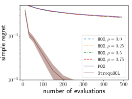
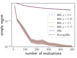
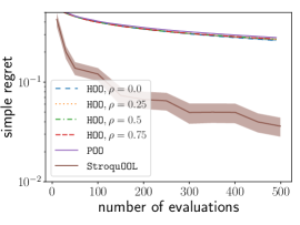
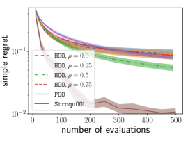
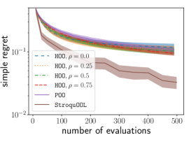
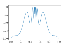
Figure 3: Bottom right: Wrapped-sine function ($d>0$). The true range of the noise $b$ and the range used by HOO and POO is $\widetilde{b}$. Top: $b=0,\widetilde{b}=1$ left — $b=0.1,\widetilde{b}=1$ middle — $b=\widetilde{b}=1$ right. Bottom: $b=\widetilde{b}=0.1$ left — $b=1,\widetilde{b}=0.1$ middle.

We use two functions used by prior work as testbeds for optimization of difficult function without the knowledge of smoothness. The first one is the wrapped-sine function ($S(x),$ Grill et al., 2015, Figure 3, bottom right) with $S(x)\triangleq\frac{1}{2}(\sin(\pi\log_{2}(2|x-\frac{1}{2}|))+1)((2|x-\frac{1}{2}|)^{-\log.8}-(2|x-\frac{1}{2}|)^{-\log.3})-(2|x-\frac{1}{2}|)^{-\log.8}$. This function has $d>0$ for the standard partitioning (Grill et al., 2015). The second is the garland function ($G(x),$ Valko et al., 2013, Figure 4, bottom right) with $G(x)\triangleq 4x(1-x)(\frac{3}{4}+\frac{1}{4}(1-\sqrt{|\sin(60x)|}))$. Function $G$ has $d=0$ for the standard partitioning (Valko et al., 2013). Both functions are in one dimension, $\mathcal{X}=\mathbb{R}$. Our algorithms work in any dimension, but, with the current computational power available, they would not scale beyond a thousand dimensions.

StroquOOL outperforms POO and HOO and adapts to lower noise.

In Figure 3, we report the results of StroquOOL, POO, and HOO for different values of $\rho$. As detailed in the caption, we vary the range of noise $b$ and the range of noise $\widetilde{b}$ used by HOO and POO. In all our experiments, StroquOOL outperforms POO and HOO. StroquOOL adapts to low noise, its performance improves when $b$ diminishes. To see that, compare top-left ($b=0$), top-middle ($b=.1$), and top-right ($b=1$) subfigures. On the other hand, POO and HOO do not naturally adapt to the range of the noise: For a given parameter $\widetilde{b}=1$, the performance is unchanged when the range of the real noise varies as seen by comparing again top-left ($b=0$), top-middle ($b=.1$), and top-right ($b=1$). However, note that POO and HOO can adapt to noise and perform empirically well if they have a good estimate of the range $b=\widetilde{b}$ as in bottom-left, or if they underestimate the range of the noise, $\widetilde{b}\ll b$, as in bottom-middle. In Figure 5, we report similar results on the garland function. Finally, StroquOOL demonstrates its adaptation to both worlds in Figure 4 (left), where it achieves exponential decreasing loss in the case $d=0$ and deterministic feedback.

Regrets of SequOOL and StroquOOL have exponential decay when $d=0$.

In Figure 4, we test in the deterministic feedback case with SequOOL, StroquOOL, SOO and the uniform strategy on the garland function (left) and the wrap-sine function (middle). Interestingly, for the garland function, where $d=0$, SequOOL outperforms SOO and displays a truly exponential regret decay (y-axis is in log scale). SOO appears to have the regret of $e^{-\sqrt{n}}$. StroquOOL which is expected to have a regret $e^{-n/\log^{2}n}$ lags behind SOO. Indeed, $n/\log^{2}n$ exceeds $\sqrt{n}$ for $n>10000$, for which the result is beyond the numerical precision. In Figure 4 (middle), we used the wrapped-sine. While all algorithms have similar theoretical guaranties since here $d>0$, SOO outperforms the other algorithms.

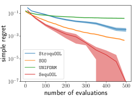
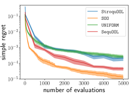
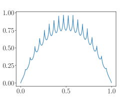
Figure 4: Left & center: Deterministic feedback. Right: Garland function for which $d=0$.

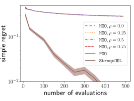
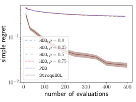
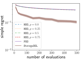
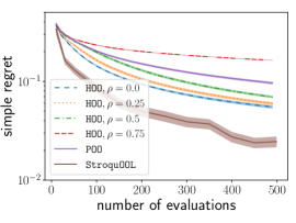
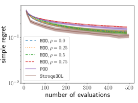
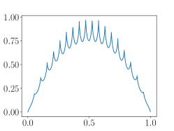
Figure 5: Garland function: The true range of the noise is $b$ and the range of noise used by HOO and POO is $\widetilde{b}$ and they are set as top: $b=0,\widetilde{b}=1$ left — $b=0.1,\widetilde{b}=1$ middle — $b=1,\widetilde{b}=1$ right, bottom: $b=0.1,\widetilde{b}=0.1$ left — $b=1,\widetilde{b}=0.1$ middle.

A more thorough empirical study is desired. Especially we would like to see how our methods compare with state-of-the-art black-box GO approaches (Pintér, 2018; Pintér et al., 2018; Strongin and Sergeyev, 2000; Sergeyev et al., 2013; Sergeyev and Kvasov, 2017, 2006; Sergeyev, 1998; Lera and Sergeyev, 2010; Kvasov and Sergeyev, 2012; Lera and Sergeyev, 2015; Kvasov and Sergeyev, 2015).

Acknowledgements

We would like to thank Jean-Bastien Grill for his code and Côme Fiegel for helpful discussions and proof reading. We gratefully acknowledge the support of the NSF through grant IIS-1619362 and of the Australian Research Council through an Australian Laureate Fellowship (FL110100281) and through the Australian Research Council Centre of Excellence for Mathematical and Statistical Frontiers (ACEMS). The research presented was also supported by European CHIST-ERA project DELTA, French Ministry of Higher Education and Research, Nord-Pas-de-Calais Regional Council, Inria and Otto-von-Guericke-Universität Magdeburg associated-team north-european project Allocate, and French National Research Agency projects ExTra-Learn (n.ANR-14-CE24-0010-01) and BoB (n.ANR-16-CE23-0003). This research has also benefited from the support of the FMJH Program PGMO and from the support to this program from Criteo.

Appendix A Regret analysis of SequOOL for deterministic feedback

See 3.3

Proof A.1.

We prove Lemma 3.3 by induction in the following sense. For a given $h$, we assume the hypotheses of the lemma for that $h$ are true and we prove by induction that $\bot_{h^{\prime}}=h^{\prime}$ for $h^{\prime}\in[h]$.
$1^{\circ}$ For $h^{\prime}=0$, we trivially have $\bot_{h^{\prime}}\geq 0$.
$2^{\circ}$ Now consider $h^{\prime}>0$ and assume $\bot_{h^{\prime}-1}=h^{\prime}-1$ with the objective to prove $\bot_{h^{\prime}}=h^{\prime}$. Therefore, at the end of the processing of depth $h^{\prime}-1$, during which we were opening the cells of depth $h^{\prime}-1$ we managed to open the cell $(h^{\prime}-1,i_{h^{\prime}-1}^{\star})$ the optimal node of depth $h^{\prime}-1$ (i.e., such that $x^{\star}\in\mathcal{P}_{h^{\prime}-1,i^{\star}_{h^{\prime}-1}})$. During phase $h^{\prime}$, the $\mathopen{}\mathclose{{}\left\lfloor\frac{h_{\rm max}}{h^{\prime}}}\right\rfloor$ cells from $\mathopen{}\mathclose{{}\left\{\mathcal{P}_{h^{\prime},i}}\right\}_{i}$ with highest values $\mathopen{}\mathclose{{}\left\{f_{h^{\prime},i}}\right\}_{i}$ are opened. For the purpose of contradiction, let us assume $\bot_{h^{\prime}}=h^{\prime}-1$ that is $\mathcal{P}_{h^{\prime},i_{h}^{\star}}$ is not one of them. This would mean that there exist at least $\mathopen{}\mathclose{{}\left\lfloor\frac{h_{\rm max}}{h^{\prime}}}\right\rfloor$ cells from $\mathopen{}\mathclose{{}\left\{\mathcal{P}_{h^{\prime},i}}\right\}_{i}$, distinct from $\mathcal{P}_{h^{\prime},i_{h}^{\star}}$, satisfying $f_{h^{\prime},i}\geq f_{h^{\prime},i^{\star}_{h}}$. As $f_{h^{\prime},i^{\star}}\geq f(x^{\star})-\nu\rho^{h^{\prime}}$ by Assumption 1, this means we have $\mathcal{N}_{h^{\prime}}(3\nu\rho^{h^{\prime}})\geq\mathopen{}\mathclose{{}\left\lfloor\frac{h_{\rm max}}{h^{\prime}}}\right\rfloor+1$ (the $+1$ is for $\mathcal{P}_{h^{\prime},i_{h}^{\star}}$). As $h^{\prime}\leq h$ this gives $\frac{h_{\rm max}}{h^{\prime}}\geq\frac{h_{\rm max}}{h}$ and therefore $\mathcal{N}_{h^{\prime}}(3\nu\rho^{h^{\prime}})\geq\mathopen{}\mathclose{{}\left\lfloor\frac{h_{\rm max}}{h}}\right\rfloor+1$. However by assumption of the lemma we have $\frac{h_{\rm max}}{h}\geq C\rho^{-d(\nu,C,\rho)h}\geq C\rho^{-d(\nu,C,\rho)h^{\prime}}$. It follows that $\mathcal{N}_{h^{\prime}}(3\nu\rho^{h^{\prime}})>\mathopen{}\mathclose{{}\left\lfloor C\rho^{-d(\nu,C,\rho)h^{\prime}}}\right\rfloor$. This contradicts $f$ being of near-optimality dimension $d(\nu,C,\rho)$ with associated constant $C$ as defined in Definition 2.1. Indeed the condition $\mathcal{N}_{h^{\prime}}(3\nu\rho^{h^{\prime}})\leq C\rho^{-dh^{\prime}}$ in Definition 2.1 is equivalent to the condition $\mathcal{N}_{h^{\prime}}(3\nu\rho^{h^{\prime}})\leq\mathopen{}\mathclose{{}\left\lfloor C\rho^{-dh^{\prime}}}\right\rfloor$ as $\mathcal{N}_{h^{\prime}}(3\nu\rho^{h^{\prime}})$ is an integer.

See 3.4 See 3.5

Proof A.2.

Let $x^{\star}$ be a global optimum with associated $(\nu,\rho)$. For simplicity, let $d=d(\nu,C,\rho)$. We have

$$f(x(n))\stackrel{{\scriptstyle\textbf{(a)}}}{{\geq}}f_{\bot_{h_{\rm max}}+1,i^{\star}}\stackrel{{\scriptstyle\textbf{(b)}}}{{\geq}}f(x^{\star})-\nu\rho^{\bot_{h_{\rm max}}+1}.$$

where (a) is because $x(\bot_{h_{\rm max}}+1,i^{\star})\in\mathcal{T}$ and $x(n)=\operatorname*{arg\,max}_{\mathcal{P}_{h,i}\in\mathcal{T}}f_{h,i}$, and (b) is by Assumption 1. Note that the tree has depth $h_{\rm max}+1$ in the end. From the previous inequality we have $r_{n}=\sup_{x\in\mathcal{X}}f\mathopen{}\mathclose{{}\left(x}\right)-f\mathopen{}\mathclose{{}\left(x(n)}\right)\leq\nu\rho^{\bot_{h_{\rm max}}+1}$. For the rest of the proof, we want to lower bound $\bot_{h_{\rm max}}$. Lemma 3.3 provides a sufficient condition on $h$ to get lower bounds. This condition is an inequality in which as $h$ gets larger (more depth) the condition is more and more likely not to hold. For our bound on the regret of SequOOL to be small, we want a quantity $h$ so that the inequality holds but having $h$ as large as possible. So it makes sense to see when the inequality flip signs which is when it turns to equality. This is what we solve next. We solve Equation 2 and then verify that it gives a valid indication of the behavior of our algorithm in term of its optimal $h$. We denote $\overline{h}$ the positive real number satisfying

$$\frac{h_{\rm max}}{\overline{h}}=C\rho^{-d\overline{h}}.$$ (2)

First we will verify that $\mathopen{}\mathclose{{}\left\lfloor\overline{h}}\right\rfloor$ is a reachable depth by SequOOL in the sense that $\overline{h}\leq h_{\rm max}$. As $\rho<1$, $d\geq 0$ and $\overline{h}\geq 0$ we have $\rho^{-d\overline{h}}\geq 1$. This gives $C\rho^{-d\overline{h}}\geq 1$. Finally as $\frac{h_{\rm max}}{\overline{h}}=C\rho^{-d\overline{h}}$, we have $\overline{h}\leq h_{\rm max}$.

If $d=0$ we have $\overline{h}=h_{\rm max}/C$. If $d>0$ we have $\overline{h}=\frac{1}{d\log(1/\rho)}W\mathopen{}\mathclose{{}\left(h_{\rm max}d\log(1/\rho)/C}\right)$ where $W$ is the standard Lambert $W$ function. Using standard properties of the $\lfloor\cdot\rfloor$ function, we have

$$\frac{h_{\rm max}}{\mathopen{}\mathclose{{}\left\lfloor\overline{h}}\right\rfloor}\geq\frac{h_{\rm max}}{\overline{h}}=C\rho^{-d\overline{h}}\geq C\rho^{-d\mathopen{}\mathclose{{}\left\lfloor\overline{h}}\right\rfloor}.$$ (3)

We always have $\bot_{h_{\rm max}}\geq 0$. If $\overline{h}\geq 1$, as discussed above $\mathopen{}\mathclose{{}\left\lfloor\overline{h}}\right\rfloor\in[h_{\rm max}]$, therefore $\bot_{h_{\rm max}}\geq\bot_{\mathopen{}\mathclose{{}\left\lfloor\overline{h}}\right\rfloor},$ as $\bot_{\cdot}$ is increasing. Moreover $\bot_{\overline{h}}=\overline{h}$ because of Lemma 3.3 which assumptions are verified because of Equation 3 and $\mathopen{}\mathclose{{}\left\lfloor\overline{h}}\right\rfloor\in[0:h_{\rm max}]$. So in general we have $\bot_{h_{\rm max}}\geq\mathopen{}\mathclose{{}\left\lfloor\overline{h}}\right\rfloor$. If $d=0$ we have, $r_{n}\leq\nu\rho^{\bot_{h_{\rm max}}+1}\leq\nu\rho^{\mathopen{}\mathclose{{}\left\lfloor\overline{h}}\right\rfloor+1}=\nu\rho^{\mathopen{}\mathclose{{}\left\lfloor\frac{h_{\rm max}}{C}}\right\rfloor+1}\leq\nu\rho^{\frac{h_{\rm max}}{C}}=\nu\rho^{\frac{1}{C}\mathopen{}\mathclose{{}\left\lfloor\frac{n}{\overline{\log}\,n}}\right\rfloor}.$

If $d>0$ $r_{n}\leq\nu\rho^{\bot_{h_{\rm max}}+1}~{}\leq~{}\nu\rho^{\frac{1}{d\log(1/\rho)}W\mathopen{}\mathclose{{}\left(\frac{h_{\rm max}d\log(1/\rho)}{C}}\right)}.$ To obtain the result in Corollary 3.5, we use that $W(x)$ verifies for $x\geq e$, $W(x)\geq\log\mathopen{}\mathclose{{}\left(\frac{x}{\log x}}\right)$ (Hoorfar and Hassani, 2008). Therefore, if $h_{\rm max}d\log(1/\rho)/C>e$ we have, denoting $d_{\rho}=d\log(1/\rho)$,

$$\frac{r_{n}}{\nu} \leq\rho^{\frac{1}{d_{\rho}}\mathopen{}\mathclose{{}\left(\log\mathopen{}\mathclose{{}\left(\frac{h_{\rm max}d_{\rho}/C}{\log\mathopen{}\mathclose{{}\left(h_{\rm max}d_{\rho}/C}\right)}}\right)}\right)}=e^{\frac{1}{d\log(1/\rho)}\mathopen{}\mathclose{{}\left(\log\mathopen{}\mathclose{{}\left(\frac{h_{\rm max}d_{\rho}/C}{\log\mathopen{}\mathclose{{}\left(\frac{h_{\rm max}d_{\rho}}{C}}\right)}}\right)}\right)\log(\rho)}=\mathopen{}\mathclose{{}\left(\frac{h_{\rm max}d_{\rho}/C}{\log\mathopen{}\mathclose{{}\left(\frac{h_{\rm max}d_{\rho}}{C}}\right)}}\right)^{-\frac{1}{d}}.$$

Appendix B StroquOOL is not using a budget larger than $n$

Summing over the depths except the depth $0$, StroquOOL never uses more evaluations than the budget $h_{\rm max}\overline{\log}^{2}(h_{\rm max})$ during this depth exploration as

$$\sum_{h=1}^{h_{\rm max}}\sum_{p=0}^{\mathopen{}\mathclose{{}\left\lfloor h_{\rm max}/h}\right\rfloor}\mathopen{}\mathclose{{}\left\lfloor\frac{h_{\rm max}}{hp}}\right\rfloor \leq\sum_{h=1}^{h_{\rm max}}\sum_{p=0}^{\mathopen{}\mathclose{{}\left\lfloor h_{\rm max}/h}\right\rfloor}\frac{h_{\rm max}}{hp}=\sum_{h=1}^{h_{\rm max}}\frac{h_{\rm max}}{h}\sum_{p=0}^{\mathopen{}\mathclose{{}\left\lfloor h_{\rm max}/h}\right\rfloor}\frac{1}{p}=\sum_{h=1}^{h_{\rm max}}\frac{h_{\rm max}}{h}\overline{\log}(\mathopen{}\mathclose{{}\left\lfloor h_{\rm max}/h}\right\rfloor)$$

$$\leq\overline{\log}(h_{\rm max})\sum_{h=1}^{h_{\rm max}}\frac{h_{\rm max}}{h}=h_{\rm max}\overline{\log}^{2}(h_{\rm max}).$$

We need to add the additional evaluations for the cross-validation at the end,

$$\sum_{p=0}^{p_{\rm max}}\frac{1}{2}\mathopen{}\mathclose{{}\left\lfloor\frac{n}{2(\overline{\log}n+1)^{2}}}\right\rfloor\leq\frac{n}{4}\cdot$$

Therefore, in total the budget is not more than $\frac{n}{2}+\frac{n}{4}+h_{\rm max}=n$.

Appendix C Lower bound on the probability of event $\xi_{\delta}$

In this section, we define and consider event $\xi_{\delta}$ and prove it holds with high probability.

Lemma C.1.

Let $\mathcal{C}$ be the set of cells evaluated by StroquOOL during one of its runs. $\mathcal{C}$ is a random quantity. Let $\xi_{\delta}$ be the event under which all average estimates in the cells receiving at least one evaluation from StroquOOL are within their classical confidence interval, then $P(\xi_{\delta})\geq 1-\delta$, where

$$\xi_{\delta}\triangleq\mathopen{}\mathclose{{}\left\{\forall\mathcal{P}_{h,i}\in\mathcal{C},\,p\in[0:p_{\rm max}]:\text{if~{} }T_{h,i}=2^{p},\text{ then }\mathopen{}\mathclose{{}\left|\widehat{f}_{h,i}-f_{h,i}}\right|\leq b\sqrt{\frac{\log(2n^{2}/\delta)}{2^{p+1}}}}\right\}\!\cdot$$

Proof C.2.

The proof of this lemma follows the proof of the equivalent statement given for StoSOO (Valko et al., 2013). The crucial point is that while we have potentially exponentially many combinations of cells that can be evaluated, given any particular execution we need to consider only a polynomial number of estimators for which we can use Chernoff-Hoeffding concentration inequality.

Let $m$ denote the (random) number of different nodes sampled by the algorithm up to time $n$. Let $\tau_{j}^{1}$ be the first time when the $j$-th new node $\mathcal{P}_{H_{j},I_{j}}$ is sampled, i.e., at time $\tau_{j}^{1}-1$ there are only $j-1$ different nodes that have been sampled whereas at time $\tau_{j}^{1}$, the $j$-th new node $\mathcal{P}_{H_{j},I_{j}}$ is sampled for the first time. Let $\tau_{j}^{s}$, for $1\leq s\leq T_{H_{j},I_{j}}(n)$, be the time when the node $\mathcal{P}_{H_{j},I_{j}}$ is sampled for the $s$-th time. Moreover, we denote $Y_{j}^{s}=y_{\tau_{j}^{s}}-f(x_{H_{j},I_{j}})$. Using this notation, we rewrite $\xi$ as:

$$\xi_{\delta}=\Bigg{\{} \forall j,p\mbox{ s.t. },1\leq i\leq m,\,p\in[0:p_{\rm max}],\text{if }T_{H_{i},J_{i}}(n)=2^{p},\bigg{|}\frac{1}{2^{p}}\sum_{s=1}^{2^{p}}Y^{s}_{j}\bigg{|}\leq\sqrt{\frac{\log(2n^{2}/\delta)}{2^{p+1}}}\Bigg{\}}.$$ (4)

Now, for any $j$ and $p$, the $(Y_{j}^{s})_{1\leq s\leq u}$ are i.i.d. from some distribution $\mathcal{P}_{H_{j},I_{j}}$. The node $\mathcal{P}_{H_{j},I_{j}}$ is random and depends on the past samples (before time $\tau_{j}^{1}$) but the $(Y_{j}^{s})_{s}$ are conditionally independent given this node and consequently:

$$\P \Bigg{(}\bigg{|}\frac{1}{2^{p}}\sum_{s=1}^{2^{p}}Y_{j}^{s}\bigg{|}\leq\sqrt{\frac{\log(2n^{2}/\delta)}{2^{p+1}}}\Bigg{)}=$$

$$=\mathbb{E}_{\mathcal{P}_{H_{j},I_{j}}}\,\P\bigg{(}\bigg{|}\frac{1}{2^{p}}\sum_{s=1}^{u}Y^{s}_{i}\bigg{|}\leq\sqrt{\frac{\log(2n^{2}/\delta)}{2^{p+1}}}\ \Bigg{|}\mathcal{P}_{H_{j},I_{j}}\bigg{)}$$

$$\geq 1-\frac{\delta}{2n},$$

using Chernoff-Hoeffding’s inequality. We finish the proof by taking a union bound over all values of $1\leq j\leq n$ and $1\leq p\leq p_{\rm max}$.

Appendix D Proof of Lemma 4.1

See 4.1

Proof D.1.

We place ourselves on event $\xi_{\delta}$ defined in Lemma C.1 and for which we proved that $P(\xi_{\delta})\geq 1-\delta$. We fix $p$. We prove the statement of the lemma, given that event $\xi_{\delta}$ holds, by induction in the following sense. For a given $h$ and $p$, we assume the hypotheses of the lemma for that $h$ and $p$ are true and we prove by induction that $\bot_{h^{\prime},p}=h^{\prime}$ for $h^{\prime}\in[h]$.
$1^{\circ}$ For $h^{\prime}=0$, we trivially have that $\bot_{h^{\prime},p}\geq 0$.
$2^{\circ}$ Now consider $h^{\prime}>0$, and assume $\bot_{h^{\prime}-1,p}=h^{\prime}-1$ with the objective to prove that $\bot_{h^{\prime},p}=h^{\prime}$. Therefore, at the end of the processing of depth $h^{\prime}-1$, during which we were opening the cells of depth $h^{\prime}-1$ we managed to open the cell $\mathcal{P}_{h^{\prime}-1,i_{h^{\prime}-1}^{\star}}$ with at least $2^{p}$ evaluations. $\mathcal{P}_{h^{\prime}-1,i_{h^{\prime}-1}^{\star}}$ is the optimal node of depth $h^{\prime}-1$ (i.e., such that $x^{\star}\in\mathcal{P}_{h^{\prime}-1,i^{\star}})$. Let $m$ be the largest integer such that $2^{p}\leq\frac{h_{\rm max}}{2h^{\prime}m}$. We have $\frac{h_{\rm max}}{2h^{\prime}m}\leq\mathopen{}\mathclose{{}\left\lfloor\frac{h_{\rm max}}{h^{\prime}m}}\right\rfloor$ and also $2^{p}\geq\frac{h_{\rm max}}{2h^{\prime}(m+1)}\geq\frac{h_{\rm max}}{4h^{\prime}m}$. During phase $h^{\prime}$, the $m$ cells from $\mathopen{}\mathclose{{}\left\{\mathcal{P}_{h^{\prime},i}}\right\}$ with highest values $\mathopen{}\mathclose{{}\left\{\widehat{f}(x_{h^{\prime},i})}\right\}_{h^{\prime},i}$ and having been evaluated at least $\mathopen{}\mathclose{{}\left\lfloor\frac{h_{\rm max}}{h^{\prime}m}}\right\rfloor\geq 2^{p}$ are opened at least $\mathopen{}\mathclose{{}\left\lfloor\frac{h_{\rm max}}{h^{\prime}m}}\right\rfloor\geq 2^{p}$ times. For the purpose of contradiction, let us assume that $\mathcal{P}_{h^{\prime},i_{h^{\prime}}^{\star}}$ is not one of them. This would mean that there exist at least $m$ cells from $\mathopen{}\mathclose{{}\left\{\mathcal{P}_{h^{\prime},i}}\right\}$, distinct from $\mathcal{P}_{h^{\prime},i_{h}^{\star}}$, satisfying $\widehat{f}_{h^{\prime},i}\geq\widehat{f}_{h^{\prime},i^{\star}_{h^{\prime}}}$ and each having been evaluated at least $2^{p}$ times. This means that, for these cells we have $f_{h^{\prime},i}+\nu\rho^{h^{\prime}}\geq f_{h^{\prime},i}+\nu\rho^{h}\stackrel{{\scriptstyle\textbf{(a)}}}{{\geq}}f_{h^{\prime},i}+b\sqrt{\frac{\log(2n^{2}/\delta)}{2^{p+1}}}\stackrel{{\scriptstyle\textbf{(b)}}}{{\geq}}\widehat{f}_{h^{\prime},i}\geq\widehat{f}_{h^{\prime},i^{\star}_{h^{\prime}}}\stackrel{{\scriptstyle\textbf{(b)}}}{{\geq}}f_{h^{\prime},i^{\star}_{h^{\prime}}}-b\sqrt{\frac{\log(2n^{2}/\delta)}{2^{p+1}}}\stackrel{{\scriptstyle\textbf{(a)}}}{{\geq}}f_{h^{\prime},i^{\star}_{h^{\prime}}}-\nu\rho^{h}\geq f_{h^{\prime},i^{\star}_{h^{\prime}}}-\nu\rho^{h^{\prime}}$, where (a) is by assumption of the lemma, (b) is because $\xi$ holds. As $f_{h^{\prime},i^{\star}_{h^{\prime}}}\geq f(x^{\star})-\nu\rho^{h^{\prime}}$ by Assumption 1, this means we have $\mathcal{N}_{h^{\prime}}(3\nu\rho^{h^{\prime}})\geq m+1\geq\frac{h_{\rm max}}{4h^{\prime}2^{p}}+1$ (the $+1$ is for $\mathcal{P}_{h^{\prime},i_{h^{\prime}}^{\star}}$). As $h^{\prime}\leq h$ this gives $\frac{h_{\rm max}}{h^{\prime}2^{p}}\geq\frac{h_{\rm max}}{h2^{p}}$ and therefore $\mathcal{N}_{h^{\prime}}(3\nu\rho^{h^{\prime}})\geq\mathopen{}\mathclose{{}\left\lfloor\frac{h_{\rm max}}{4h2^{p}}}\right\rfloor+1$. However by assumption of the lemma we have $\frac{h_{\rm max}}{4h2^{p}}\geq C\rho^{-d(\nu,C,\rho)h}\geq C\rho^{-d(\nu,C,\rho)h^{\prime}}$. It follows that $\mathcal{N}_{h^{\prime}}(3\nu\rho^{h^{\prime}})>\mathopen{}\mathclose{{}\left\lfloor C\rho^{-d(\nu,C,\rho)h^{\prime}}}\right\rfloor$. This leads to having a contradiction with the function $f$ being of near-optimality dimension $d(\nu,C,\rho)$ as defined in Definition 2.1. Indeed, the condition $\mathcal{N}_{h^{\prime}}(3\nu\rho^{h^{\prime}})\leq C\rho^{-dh^{\prime}}$ in Definition 2.1 is equivalent to the condition $\mathcal{N}_{h^{\prime}}(3\nu\rho^{h^{\prime}})\leq\mathopen{}\mathclose{{}\left\lfloor C\rho^{-dh^{\prime}}}\right\rfloor$ as $\mathcal{N}_{h^{\prime}}(3\nu\rho^{h^{\prime}})$ is an integer. Reaching the contradiction proves the claim of the lemma.

Appendix E Proof of Theorem 4.2 and Theorem 4.4

See 4.2 See 4.4

Proof E.1 (Proof of Theorem 4.2 and Theorem 4.4).

We first place ourselves on the event $\xi$ defined in Lemma C.1 and where it is proven that $P(\xi)\geq 1-\delta$. We bound the simple regret of StroquOOL on $\xi$. We consider a global optimum $x^{\star}$ with associated $(\nu,\rho)$. For simplicity we write $d=d(\nu,C,\rho)$. We have for all $p\in[0:p_{\rm max}]$

$$f(x(n)) +b\sqrt{\frac{\log(2n^{2}/\delta)}{h_{\rm max}}}\stackrel{{\scriptstyle\textbf{(a)}}}{{\geq}}\widehat{f}(x(n))\stackrel{{\scriptstyle\textbf{(c)}}}{{\geq}}\widehat{f}(x(n,p))\stackrel{{\scriptstyle\textbf{(b)}}}{{\geq}}\widehat{f}\mathopen{}\mathclose{{}\left(x(\bot_{h_{\rm max},p}+1,i^{\star})}\right)$$

$$\stackrel{{\scriptstyle\textbf{(a)}}}{{\geq}}f(x(\bot_{h_{\rm max},p}+1,i^{\star}))-b\sqrt{\frac{\log(2n^{2}/\delta)}{h_{\rm max}}}\stackrel{{\scriptstyle\textbf{(d)}}}{{\geq}}f\mathopen{}\mathclose{{}\left(x^{\star}}\right)-\nu\rho^{\bot_{h_{\rm max},p}+1}-b\sqrt{\frac{\log(2n^{2}/\delta)}{h_{\rm max}}}$$

where (a) is because the $x(n,p)$ are evaluated $h_{\rm max}$ times at the end of StroquOOL and because $\xi$ holds, (b) is because $x_{\bot_{h_{\rm max},p}+1,i^{\star}}\in\{\mathopen{}\mathclose{{}\left(h,i}\right)\in\mathcal{T},T_{h,i}\geq 2^{p}\}$ and $x(n,p)=\operatorname*{arg\,max}\limits_{\mathcal{P}_{h,i}\in\mathcal{T},T_{h,i}\geq 2^{p}}\widehat{f}_{h,i}$, (c) is because $x(n)=\operatorname*{arg\,max}\limits_{\{x(n,p),p\in[0:p_{\rm max}]\}}\widehat{f}(x(n,p))$, and (d) is by Assumption 1.

From the previous inequality we have $r_{n}=f\mathopen{}\mathclose{{}\left(x^{\star}}\right)-f\mathopen{}\mathclose{{}\left(x(n)}\right)\leq\nu\rho^{\bot_{h_{\rm max},p}+1}+2b\sqrt{\frac{\log(2n^{2}/\delta)}{h_{\rm max}}}$, for $p\in[0:p_{\rm max}]$.

For the rest of proof we want to lower bound $\max_{p\in[0:p_{\rm max}]}\bot_{h_{\rm max},p}$. Lemma 4.1 provides some sufficient conditions on $p$ and $h$ to get lower bounds. These conditions are inequalities in which as $p$ gets smaller (fewer samples) or $h$ gets larger (more depth) these conditions are more and more likely not to hold. For our bound on the regret of StroquOOL to be small, we want quantities $p$ and $h$ where the inequalities hold but using as few samples as possible (small $p$) and having $h$ as large as possible. Therefore we are interested in determining when the inequalities flip signs which is when they turn to equalities. This is what we solve next. We denote $\widetilde{h}$ and $\widetilde{p}$ the real numbers satisfying

$$\frac{h_{\rm max}\nu^{2}\rho^{2\widetilde{h}}}{4\widetilde{h}b^{2}\log(2n^{2}/\delta)}=C\rho^{-d\widetilde{h}}\quad\text{and}\quad b\sqrt{\frac{\log(2n^{2}/\delta)}{2^{\widetilde{p}}}}=\nu\rho^{\widetilde{h}}.$$ (5)

Our approach is to solve Equation 5 and then verify that it gives a valid indication of the behavior of our algorithm in term of its optimal $p$ and $h$. We have

$$\widetilde{h}=\frac{1}{(d+2)\log(1/\rho)}W\mathopen{}\mathclose{{}\left(\frac{\nu^{2}h_{\rm max}(d+2)\log(1/\rho)}{4Cb^{2}\log(2n^{2}/\delta)}}\right)$$

where standard $W$ is the Lambert $W$ function.

However after a close look at the Equation 5, we notice that it is possible to get values $\widetilde{p}<0$ which would lead to a number of evaluations $2^{p}<1$. This actually corresponds to an interesting case when the noise has a small range and where we can expect to obtain an improved result, that is: obtain a regret rate close to the deterministic case. This low range of noise case then has to be considered separately.

Therefore, we distinguish two cases which corresponds to different noise regimes depending on the value of $b$. Looking at the equation on the right of (5), we have that $\widetilde{p}<0$ if $\frac{\nu^{2}\rho^{2\widetilde{h}}}{b^{2}\log(2n^{2}/\delta)}>1$. Based on this condition we now consider the two cases. However for both of them we define some generic $\ddot{h}$ and $\ddot{p}$.

High-noise regime $\frac{\nu^{2}\rho^{2\widetilde{h}}}{b^{2}\log(2n^{2}/\delta)}\leq 1$:

In this case, we denote $\ddot{h}=\widetilde{h}$ and $\ddot{p}=\widetilde{p}$. As $\frac{1}{2^{\widetilde{p}}}=\frac{\nu^{2}\rho^{2\widetilde{h}}}{b^{2}\log(2n^{2}/\delta)}\leq 1$ by construction, we have $\widetilde{p}\geq 0$. Using standard properties of the $\lfloor\cdot\rfloor$ function, we have

$$b\sqrt{\frac{\log(2n^{2}/\delta)}{2^{\mathopen{}\mathclose{{}\left\lfloor\widetilde{p}}\right\rfloor+1}}}\leq b\sqrt{\frac{\log(2n^{2}/\delta)}{2^{\widetilde{p}}}}=\nu\rho^{\widetilde{h}}\leq\nu\rho^{\mathopen{}\mathclose{{}\left\lfloor\widetilde{h}}\right\rfloor}$$ (6)

$$\text{ and,~{}~{} }\frac{h_{\rm max}}{4\mathopen{}\mathclose{{}\left\lfloor\widetilde{h}}\right\rfloor 2^{\mathopen{}\mathclose{{}\left\lfloor\widetilde{p}}\right\rfloor}}\geq\frac{h_{\rm max}}{4\mathopen{}\mathclose{{}\left\lfloor\widetilde{h}}\right\rfloor 2^{\widetilde{p}}}=\frac{h_{\rm max}\nu^{2}\rho^{2\widetilde{h}}}{4\mathopen{}\mathclose{{}\left\lfloor\widetilde{h}}\right\rfloor b^{2}\log(2n^{2}/\delta)}\geq\frac{h_{\rm max}\nu^{2}\rho^{2\widetilde{h}}}{4\widetilde{h}b^{2}\log(2n^{2}/\delta)}=C\rho^{-d\widetilde{h}}\geq C\rho^{-d\mathopen{}\mathclose{{}\left\lfloor\widetilde{h}}\right\rfloor}.$$ (7)

Low-noise regime $\frac{\nu^{2}\rho^{2\widetilde{h}}}{b^{2}\log(2n^{2}/\delta)}>1$ or $b=0$:

In this case, we can reuse arguments close to the argument used in the deterministic feedback case in the proof of SequOOL (Theorem 3.4), we denote $\ddot{h}=\overline{h}$ and $\ddot{p}=\overline{p}$ where $\overline{h}$ and $\overline{p}$ verify,

$$\frac{h_{\rm max}}{4\overline{h}}=C\rho^{-d\overline{h}}\quad\text{and}\quad\overline{p}=0.$$ (8)

If $d=0$ we have $\overline{h}=h_{\rm max}/C$. If $d>0$ we have $\overline{h}=\frac{1}{d\log(1/\rho)}W\mathopen{}\mathclose{{}\left(\frac{h_{\rm max}d\log(1/\rho)}{4C}}\right)$ where standard $W$ is the standard Lambert $W$ function. Using standard properties of the $\lfloor\cdot\rfloor$ function, we have

$$b\sqrt{\frac{\log(2n^{2}/\delta)}{2^{\mathopen{}\mathclose{{}\left\lfloor\ddot{p}}\right\rfloor+1}}}\leq b\sqrt{\log(2n^{2}/\delta)}<\nu\rho^{\widetilde{h}}\stackrel{{\scriptstyle\textbf{(a)}}}{{\leq}}\nu\rho^{\overline{h}}\leq\nu\rho^{\mathopen{}\mathclose{{}\left\lfloor\overline{h}}\right\rfloor}$$ (9)

where (a) is because of the following reasoning. First note that one can assume $b>0$ as for the case $b=0$, the Equation 9 is trivial. As we have $\frac{h_{\rm max}\nu^{2}\rho^{2\widetilde{h}}}{4\widetilde{h}b^{2}\log(2n^{2}/\delta)}=C\rho^{-d\widetilde{h}}$ and $\frac{\nu^{2}\rho^{2\widetilde{h}}}{b^{2}\log(2n^{2}/\delta)}>1$, then, $\frac{h_{\rm max}}{4\widetilde{h}}<C\rho^{-d\widetilde{h}}$. From the inequality $\frac{h_{\rm max}}{4\widetilde{h}}<C\rho^{-d\widetilde{h}}$ and the fact that $\overline{h}$ corresponds to the case of equality $\frac{h_{\rm max}}{4\overline{h}}=C\rho^{-d\overline{h}}$, we deduce that $\overline{h}\leq\widetilde{h}$, since the left term of the inequality decreases with $h$ while the right term increases. Having $\overline{h}\leq\widetilde{h}$ gives $\rho^{\overline{h}}\geq\rho^{\widetilde{h}}$.

Given these particular definitions of $\ddot{h}$ and $\ddot{p}$ in two distinct cases we now bound the regret.

First we will verify that $\mathopen{}\mathclose{{}\left\lfloor\ddot{h}}\right\rfloor$ is a reachable depth by StroquOOL in the sense that $\ddot{h}\leq h_{\rm max}$ and $\ddot{p}\leq\log_{2}(h_{\rm max}/h)$ for all $h\leq\ddot{h}$. As $\rho<1$, $d\geq 0$ and $\ddot{h}\geq 0$ we have $\rho^{-d\ddot{h}}\geq 1$. This gives $C\rho^{-d\ddot{h}}\geq 1$. Finally as $\frac{h_{\rm max}}{\ddot{h}2^{\ddot{p}}}=C\rho^{-d\ddot{h}}$, we have $\ddot{h}\leq h_{\rm max}/2^{\ddot{p}}$. Note also that from the previous equation we have that if $\ddot{h}\geq 1$, $\ddot{p}\leq\log_{2}(h_{\rm max}/h)$ for all $h\leq\ddot{h}$ . Finally in both regimes we already proved that $\ddot{p}\geq 0$.

We always have $\bot_{h_{\rm max},\mathopen{}\mathclose{{}\left\lfloor\ddot{p}}\right\rfloor}\geq 0$. If $\ddot{h}\geq 1$, as discussed above $\mathopen{}\mathclose{{}\left\lfloor\ddot{h}}\right\rfloor\in\mathopen{}\mathclose{{}\left[h_{\rm max}}\right]$, therefore $\bot_{h_{\rm max},\mathopen{}\mathclose{{}\left\lfloor\ddot{p}}\right\rfloor}\geq\bot_{\mathopen{}\mathclose{{}\left\lfloor\ddot{h}}\right\rfloor,\mathopen{}\mathclose{{}\left\lfloor\ddot{p}}\right\rfloor},$ as $\bot_{\cdot,\mathopen{}\mathclose{{}\left\lfloor p}\right\rfloor}$ is increasing for all $p\in[0,p_{\rm max}]$. Moreover on event $\xi$, $\bot_{\mathopen{}\mathclose{{}\left\lfloor\ddot{h}}\right\rfloor,\mathopen{}\mathclose{{}\left\lfloor\ddot{p}}\right\rfloor}=\mathopen{}\mathclose{{}\left\lfloor\ddot{h}}\right\rfloor$ because of Lemma 4.1 which assumptions on $\mathopen{}\mathclose{{}\left\lfloor\ddot{h}}\right\rfloor$ and $\mathopen{}\mathclose{{}\left\lfloor\ddot{p}}\right\rfloor$ are verified because of Equations 6 and 7 in the high-noise regime and because of Equations 8 and 9 in the low-noise regime, and, in general, $\mathopen{}\mathclose{{}\left\lfloor\ddot{h}}\right\rfloor\in\mathopen{}\mathclose{{}\left[\mathopen{}\mathclose{{}\left\lfloor h_{\rm max}/2^{\ddot{p}}}\right\rfloor}\right]$ and $\mathopen{}\mathclose{{}\left\lfloor\ddot{p}}\right\rfloor\in[0:p_{\rm max}]$. So in general we have $\bot_{\mathopen{}\mathclose{{}\left\lfloor h_{\rm max}/2^{\ddot{p}}}\right\rfloor,\mathopen{}\mathclose{{}\left\lfloor\ddot{p}}\right\rfloor}\geq\mathopen{}\mathclose{{}\left\lfloor\ddot{h}}\right\rfloor$.

We can now bound the regret in the two regimes.

High-noise regime

In general, we have, on event $\xi$,

$$r_{n} ~{}\leq~{}\nu\rho^{\frac{1}{(d+2)\log(1/\rho)}W\mathopen{}\mathclose{{}\left(\frac{\nu^{2}h_{\rm max}(d+2)\log(1/\rho)}{C\log(2n^{2}/\delta)}}\right)}+2b\sqrt{\frac{\log(2n^{2}/\delta)}{h_{\rm max}}}\cdot$$

While in the deterministic feedback case, the regret was scaling with $d$ when $d\geq 0$, in the stochastic feedback case, the regret scale with $d+2$. This is because the uncertainty due to the presence of noise diminishes as $n^{-\frac{1}{2}}$ when we collect $n$ observations.

Moreover, as proved by Hoorfar and Hassani (2008), the Lambert $W(x)$ function verifies for $x\geq e$, $W(x)\geq\log\mathopen{}\mathclose{{}\left(\frac{x}{\log x}}\right)$. Therefore, if $\frac{\nu^{2}h_{\rm max}(d+2)\log(1/\rho)}{4C\log(2n^{2}/\delta)}>e$ we have, denoting $d^{\prime}=(d+2)\log(1/\rho)$,

$$r_{n}-2b\sqrt{\frac{\log(2n^{2}/\delta)}{h_{\rm max}}} \leq\nu\rho^{\frac{1}{d^{\prime}}\mathopen{}\mathclose{{}\left(\log\mathopen{}\mathclose{{}\left(\frac{\frac{h_{\rm max}d^{\prime}\nu^{2}}{4C\log(2n^{2}/\delta)}}{\log\mathopen{}\mathclose{{}\left(\frac{h_{\rm max}d^{\prime}\nu^{2}}{4C\log(2n^{2}/\delta)}}\right)}}\right)}\right)}$$

$$=\nu e^{\frac{1}{(d+2)\log(1/\rho)}\mathopen{}\mathclose{{}\left(\log\mathopen{}\mathclose{{}\left(\frac{\frac{h_{\rm max}d^{\prime}\nu^{2}}{4C\log(2n^{2}/\delta)}}{\log\mathopen{}\mathclose{{}\left(\frac{h_{\rm max}d^{\prime}\nu^{2}}{4C\log(2n^{2}/\delta)}}\right)}}\right)}\right)\log(\rho)}=\nu\mathopen{}\mathclose{{}\left(\frac{\frac{h_{\rm max}d^{\prime}\nu^{2}}{4C\log(2n^{2}/\delta)}}{\log\mathopen{}\mathclose{{}\left(\frac{h_{\rm max}d^{\prime}\nu^{2}}{4C\log(2n^{2}/\delta)}}\right)}}\right)^{-\frac{1}{d+2}}.$$

Low-noise regime

We have $2b\sqrt{\frac{\log(2n^{2}/\delta)}{h_{\rm max}}}\leq 2\frac{\nu\rho^{\widetilde{h}}}{\sqrt{\log(2n^{2}/\delta)}}\sqrt{\frac{\log(2n^{2}/\delta)}{h_{\rm max}}}\leq 2\nu\rho^{\widetilde{h}}\leq 2\nu\rho^{\overline{h}}$. Therefore $r_{n}\leq\nu\rho^{\bot_{h_{\rm max},\overline{p}}+1}+2b\sqrt{\frac{\log(2n^{2}/\delta)}{h_{\rm max}}}\leq 3\nu\rho^{\overline{h}}$. Discriminating between $d=0$ and $d>0$ leads to the claimed results.

Results in Expectation

We want to obtain additionally, our final result as an upper bound on the expected simple regret $\mathbb{E}r_{n}$. Compared to the results in high probability, the following extra assumption that the function $f$ is bounded is made: For all $x\in\mathcal{X},|f(x)|\leq f_{\max}$. Then $\delta$ is set as $\delta=\frac{4b}{f_{\max}\sqrt{n}}$. We bound the expected regret now discriminating on whether or not the event $\xi$ holds. We have

$$\mathbb{E}r_{n} \leq(1-\delta)\mathopen{}\mathclose{{}\left(\nu\rho^{\bot_{h_{\rm max},\ddot{p}}+1}+2b\sqrt{\frac{\log(f_{\max}n^{5/2}/b)}{h_{\rm max}}}}\right)+\delta\times f_{\max}$$

$$\leq\nu\rho^{\bot_{h_{\rm max},\ddot{p}}+1}+2b\sqrt{\frac{\log(f_{\max}n^{5/2}/b)}{h_{\rm max}}}+\frac{4b}{\sqrt{n}}$$

$$\leq\nu\rho^{\bot_{h_{\rm max},\ddot{p}}+1}+6b\sqrt{\frac{\log(f_{\max}n^{5/2}/b)}{h_{\rm max}}}\cdot$$

References

- Abbasi-Yadkori et al. (2018) Yasin Abbasi-Yadkori, Peter Bartlett, Victor Gabillon, Alan Malek, and Michal Valko. Best of both worlds: Stochastic & adversarial best-arm identification. In Conference on Learning Theory, 2018.
- Al-Dujaili and Suresh (2018) Abdullah Al-Dujaili and S. Suresh. Multi-objective simultaneous optimistic optimization. Information Sciences, 424:159–174, 2018.
- Audibert et al. (2010) Jean-Yves Audibert, Sébastien Bubeck, and Rémi Munos. Best arm identification in multi-armed bandits. In Conference on Learning Theory, pages 41–53, 2010.
- Auer et al. (2007) Peter Auer, Ronald Ortner, and Csaba Szepesvári. Improved rates for the stochastic continuum-armed bandit problem. In Conference on Computational Learning Theory, pages 454–468. Springer, 2007.
- Azar et al. (2014) Mohammad Gheshlaghi Azar, Alessandro Lazaric, and Emma Brunskill. Online stochastic optimization under correlated bandit feedback. In International Conference on Machine Learning, 2014.
- Bubeck and Slivkins (2012) Sébastien Bubeck and Aleksandrs Slivkins. The best of both worlds: stochastic and adversarial bandits. In Conference on Learning Theory, pages 42–1, 2012.
- Bubeck et al. (2011a) Sébastien Bubeck, Rémi Munos, Gilles Stoltz, and Csaba Szepesvári. X-armed bandits. Journal of Machine Learning Research, 12:1587–1627, 2011a.
- Bubeck et al. (2011b) Sébastien Bubeck, Gilles Stoltz, and Jia Yuan Yu. Lipschitz Bandits without the Lipschitz Constant. In Algorithmic Learning Theory, 2011b.
- Buşoniu and Morărescu (2014) Lucian Buşoniu and Irinel-Constantin Morărescu. Consensus for black-box nonlinear agents using optimistic optimization. Automatica, 50(4):1201–1208, 2014.
- Buşoniu et al. (2013) Lucian Buşoniu, Alexander Daniels, Rémi Munos, and Robert Babuska. Optimistic planning for continuous-action deterministic systems. In Adaptive Dynamic Programming And Reinforcement Learning (ADPRL), 2013 IEEE Symposium on, pages 69–76. IEEE, 2013.
- Coquelin and Munos (2007) Pierre-Arnaud Coquelin and Rémi Munos. Bandit algorithms for tree search. In Uncertainty in Artificial Intelligence, 2007.
- de Freitas et al. (2012) Nando de Freitas, Alex Smola, and Masrour Zoghi. Exponential regret bounds for Gaussian process bandits with deterministic observations. In International Conference on Machine Learning, 2012.
- De Rooij et al. (2014) Steven De Rooij, Tim Van Erven, Peter D Grünwald, and Wouter M Koolen. Follow the leader if you can, hedge if you must. The Journal of Machine Learning Research, 15(1):1281–1316, 2014.
- Derbel and Preux (2015) Bilel Derbel and Philippe Preux. Simultaneous optimistic optimization on the noiseless BBOB testbed. In IEEE Congress on Evolutionary Computation, CEC 2015, Sendai, Japan, May 25-28, 2015, pages 2010–2017, 2015.
- Grill et al. (2015) Jean-Bastien Grill, Michal Valko, and Rémi Munos. Black-box optimization of noisy functions with unknown smoothness. In Advances in Neural Information Processing Systems, pages 667–675, 2015.
- Hansen and Walster (2003) Eldon Hansen and G William Walster. Global optimization using interval analysis: revised and expanded, volume 264. CRC Press, 2003.
- Hoorfar and Hassani (2008) Abdolhossein Hoorfar and Mehdi Hassani. Inequalities on the lambert w function and hyperpower function. Journal of Inequalities in Pure and Applied Mathematics (JIPAM), 9(2):5–9, 2008.
- Hren and Munos (2008) Jean-Francois Hren and Rémi Munos. Optimistic Planning of Deterministic Systems. In European Workshop on Reinforcement Learning, 2008.
- Jones et al. (1993) David Jones, Cary Perttunen, and Bruce Stuckman. Lipschitzian optimization without the Lipschitz constant. Journal of Optimization Theory and Applications, 79(1):157–181, 1993.
- Kasim and Norreys (2016) Muhammad F Kasim and Peter A Norreys. Infinite dimensional optimistic optimisation with applications on physical systems. arXiv preprint arXiv:1611.05845, 2016.
- Kawaguchi et al. (2015) Kenji Kawaguchi, Leslie Pack Kaelbling, and Tomás Lozano-Pérez. Bayesian optimization with exponential convergence. In Advances in neural information processing systems, pages 2809–2817, 2015.
- Kawaguchi et al. (2016) Kenji Kawaguchi, Yu Maruyama, and Xiaoyu Zheng. Global continuous optimization with error bound and fast convergence. Journal of Artificial Intelligence Research, 56:153–195, 2016.
- Kearfott (2013) R Baker Kearfott. Rigorous global search: continuous problems, volume 13. Springer Science & Business Media, 2013.
- Kleinberg et al. (2008) Robert Kleinberg, Aleksandrs Slivkins, and Eli Upfal. Multi-armed bandits in metric spaces. In ACM Symposium on Theory of Computing (STOC), pages 681–690. ACM, 2008.
- Kocsis and Szepesvári (2006) Levente Kocsis and Csaba Szepesvári. Bandit-based Monte-Carlo planning. In European Conference on Machine Learning, 2006.
- Kvasov and Sergeyev (2012) Dmitri E Kvasov and Yaroslav D Sergeyev. Lipschitz gradients for global optimization in a one-point-based partitioning scheme. Journal of Computational and Applied Mathematics, 236(16):4042–4054, 2012.
- Kvasov and Sergeyev (2015) Dmitri E Kvasov and Yaroslav D Sergeyev. Deterministic approaches for solving practical black-box global optimization problems. Advances in Engineering Software, 80:58–66, 2015.
- Lera and Sergeyev (2010) Daniela Lera and Yaroslav D Sergeyev. An information global minimization algorithm using the local improvement technique. Journal of Global Optimization, 48(1):99–112, 2010.
- Lera and Sergeyev (2015) Daniela Lera and Yaroslav D Sergeyev. Deterministic global optimization using space-filling curves and multiple estimates of lipschitz and hölder constants. Communications in Nonlinear Science and Numerical Simulation, 23(1-3):328–342, 2015.
- Locatelli and Carpentier (2018) Andrea Locatelli and Alexandra Carpentier. Adaptivity to Smoothness in X-armed bandits. In Conference on Learning Theory, 2018.
- Malherbe and Vayatis (2017) Cédric Malherbe and Nicolas Vayatis. Global optimization of lipschitz functions. In Proceedings of the 34th International Conference on Machine Learning, pages 2314–2323, 2017.
- Maurer and Pontil (2009) Andreas Maurer and Massimiliano Pontil. Empirical bernstein bounds and sample variance penalization. In Conference on Learning Theory, 2009.
- Munos (2011) Rémi Munos. Optimistic optimization of a deterministic function without the knowledge of its smoothness. In Advances in Neural Information Processing Systems, pages 783–791, 2011.
- Munos (2014) Rémi Munos. From bandits to Monte-Carlo tree search: The optimistic principle applied to optimization and planning. Foundations and Trends in Machine Learning, 7(1):1–130, 2014.
- Pintér (1996) János D Pintér. Global optimization in action. continous and lipschitz optimization: Algorithms, implementations and applications. Kluwer Academic Publishers: Boston, 1996.
- Pintér (2018) János D Pintér. How difficult is nonlinear optimization? a practical solver tuning approach, with illustrative results. Annals of Operations Research, 265(1):119–141, 2018.
- Pintér et al. (2018) János D Pintér, Frank J Kampas, and Ignacio Castillo. Globally optimized packings of non-uniform size spheres in : a computational study. Optimization Letters, 12(3):585–613, 2018.
- Powers (1998) David Powers. Applications and explanations of Zipf’s law. In New methods in language processing and computational natural language learning. Association for Computational Linguistics, 1998.
- Preux et al. (2014) Philippe Preux, Rémi Munos, and Michal Valko. Bandits attack function optimization. In Evolutionary Computation (CEC), 2014 IEEE Congress on, pages 2245–2252. IEEE, 2014.
- Qian and Yu (2016) Hong Qian and Yang Yu. Scaling simultaneous optimistic optimization for high-dimensional non-convex functions with low effective dimensions. In AAAI, pages 2000–2006, 2016.
- Seldin and Slivkins (2014) Yevgeny Seldin and Aleksandrs Slivkins. One practical algorithm for both stochastic and adversarial bandits. In International Conference on Machine Learning, pages 1287–1295, 2014.
- Sergeyev (1998) Yaroslav D Sergeyev. Global one-dimensional optimization using smooth auxiliary functions. Mathematical Programming, 81(1):127–146, 1998.
- Sergeyev and Kvasov (2006) Yaroslav D Sergeyev and Dmitri E Kvasov. Global search based on efficient diagonal partitions and a set of lipschitz constants. SIAM Journal on Optimization, 16(3):910–937, 2006.
- Sergeyev and Kvasov (2017) Yaroslav D Sergeyev and Dmitri E Kvasov. Deterministic global optimization: An introduction to the diagonal approach. Springer, 2017.
- Sergeyev et al. (2013) Yaroslav D Sergeyev, Roman G Strongin, and Daniela Lera. Introduction to global optimization exploiting space-filling curves. Springer Science & Business Media, 2013.
- Shang et al. (2019) Xuedong Shang, Emilie Kaufmann, and Michal Valko. General parallel optimization without metric. In Algorithmic Learning Theory, 2019.
- Slivkins (2011) Aleksandrs Slivkins. Multi-armed bandits on implicit metric spaces. In Neural Information Processing Systems, 2011.
- Strongin and Sergeyev (2000) Roman Strongin and Yaroslav Sergeyev. Global Optimization with Non-Convex Constraints: Sequential and Parallel Algorithms. Nonconvex Optimization and Its Applications. Springer, 2000.
- Valko et al. (2013) Michal Valko, Alexandra Carpentier, and Rémi Munos. Stochastic simultaneous optimistic optimization. In International Conference on Machine Learning, pages 19–27, 2013.
- Wang et al. (2014) Ziyu Wang, Babak Shakibi, Lin Jin, and Nando de Freitas. Bayesian Multi-Scale Optimistic Optimization. In International Conference on Artificial Intelligence and Statistics, 2014.