Abstract

We focus on an efficient approach for quantification of uncertainty in complex chemical reaction networks with a large number of uncertain parameters and input conditions. Parameter dimension reduction is accomplished by computing an active subspace that predominantly captures the variability in the quantity of interest (QoI). In the present work, we compute the active subspace for a H₂/O₂ mechanism that involves 19 chemical reactions, using an efficient iterative strategy. The active subspace is first computed for a 19-parameter problem wherein only the uncertainty in the pre-exponents of the individual reaction rates is considered. This is followed by the analysis of a 36-dimensional case wherein the activation energies and initial conditions are also considered uncertain. In both cases, a 1-dimensional active subspace is observed to capture the uncertainty in the QoI, which indicates enormous potential for efficient statistical analysis of complex chemical systems. In addition, we explore links between active subspaces and global sensitivity analysis, and exploit these links for identification of key contributors to the variability in the model response.

Keywords: Chemical kinetics; epistemic uncertainty; active subspace; dimension reduction; surrogate

1 Introduction

Time evolution of a chemically reacting system is largely dependent upon rate constants associated with individual reactions. The rate constants are typically assumed to exhibit a certain correlation with temperature (e.g., Arrhenius-type). Hence, accurate specification of the rate-controlling parameters is critical to the fidelity of simulations. However, in practical applications, these parameters are either specified using expert knowledge or estimated based on a regression fit to a set of sparse and noisy data [1, 2, 3, 4]. Intensive research efforts in recent years within the field of uncertainty quantification (UQ) address the quantification and propagation of uncertainty in system models due to inadequate data, parametric uncertainty, and model errors [5, 6, 7, 8, 9, 10, 11].

In complex mechanisms involving a large number of reactions, characterizing the propagation of uncertainty from a large set of inputs to the model output is challenging due to the associated computational effort. A major focus of this article is the implementation of a robust framework that aims to identify important directions in the input space that predominantly capture the variability in the model output. These directions, which constitute the so called active subspace [12], are the dominant eigenvectors of a matrix derived from the gradient information of the model output with respect to an input. The active subspace methodology thus focuses on reducing the dimensionality of the problem, and hence the computational effort associated with uncertainty propagation. The focus here is on input parameter dimension reduction. This is different from techniques such at Computational Singular Perturbation (CSP) [13, 14, 15, 16, 17] that aim to reduce the complexity of stiff chemical systems by filtering out the fast timescales from the system. The latter is done, for instance, using the eigenvectors of the system Jacobian to decouple the fast and slow processes; see e.g., [16].

The application problem considered in this work is the H₂/O₂ reaction mechanism from [18]. This mechanism has gained a lot of attention as a potential source of clean energy for locomotive applications [19], and more recently in fuel cells [20, 21]. The mechanism involves 19 reactions including chain reactions, dissociation/recombination reactions, and formation and consumption of intermediate species; see Table 1. For each reaction, the reaction rate is assumed to follow an Arrhenius correlation with temperature:

$$k_{i}(T)=A_{i}T^{n_{i}}\exp(-E_{a,i}/RT),$$ (1)

where $A_{i}$ is the pre-exponent, $n_{i}$ is the temperature exponent, $E_{a,i}$ is the activation energy corresponding to the $i^{th}$ reaction, and $R$ is the universal gas constant. The Arrhenius rate law in (1) is often interpreted in a logarithmic form as follows:

$$\log(k_{i})=\log(A_{i})+n_{i}\log(T)-E_{a,i}/RT.$$ (2)

Reaction #	Reaction
$\mathcal{R}_{1}$	H + O2	$\rightleftharpoons$	O + OH
$\mathcal{R}_{2}$	O + H2	$\rightleftharpoons$	H + OH
$\mathcal{R}_{3}$	H2 + OH	$\rightleftharpoons$	H2O + H
$\mathcal{R}_{4}$	OH + OH	$\rightleftharpoons$	O + H2O
$\mathcal{R}_{5}$	H2 + M	$\rightleftharpoons$	H + H + M
$\mathcal{R}_{6}$	O + O + M	$\rightleftharpoons$	O2 + M
$\mathcal{R}_{7}$	O + H + M	$\rightleftharpoons$	OH + M
$\mathcal{R}_{8}$	H + OH +M	$\rightleftharpoons$	H2O + M
$\mathcal{R}_{9}$	H + O2 + M	$\rightleftharpoons$	HO2 + M
$\mathcal{R}_{10}$	HO2 + H	$\rightleftharpoons$	H2 + O2
$\mathcal{R}_{11}$	HO2 + H	$\rightleftharpoons$	OH + OH
$\mathcal{R}_{12}$	HO2 + O	$\rightleftharpoons$	O2 + OH
$\mathcal{R}_{13}$	HO2 + OH	$\rightleftharpoons$	H2O + O2
$\mathcal{R}_{14}$	HO2 + HO2	$\rightleftharpoons$	H2O2 + O2
$\mathcal{R}_{15}$	H2O2 + M	$\rightleftharpoons$	OH + OH + M
$\mathcal{R}_{16}$	H2O2 + H	$\rightleftharpoons$	H2O + OH
$\mathcal{R}_{17}$	H2O2 + H	$\rightleftharpoons$	HO2 + H2
$\mathcal{R}_{18}$	H2O2 + O	$\rightleftharpoons$	OH + HO2
$\mathcal{R}_{19}$	H2O2 + OH	$\rightleftharpoons$	HO2 + H2O

Table 1: Reaction mechanism for H₂/O₂ from [18]

.

The global reaction associated with the H₂/O₂ mechanism can be considered as follows:

$$2\text{H}_{2}+\text{O}_{2}\rightarrow 2\text{H}_{2}\text{O}.$$ (3)

The equivalence ratio ($\Phi$) is given as follows:

$$\Phi=\frac{(M_{\text{H}_{2}}/M_{\text{O}_{2}})_{\text{obs}}}{(M_{\text{H}_{2}}/M_{\text{O}_{2}})_{\text{st}}},$$ (4)

where the numerator on the right-hand-side denotes the ratio of the fuel (H₂) and oxidizer (O₂) at a given condition to the same quantity under stoichiometric conditions. In this study, computations were performed at fuel-rich conditions, $\Phi$ = 2.0. Homogeneous ignition at constant pressure is simulated using the TChem software package [22] using an initial pressure, $P_{0}$ = 1 atm and initial temperature, $T_{0}$ = 900 K. The time required for the rate of temperature increase to exceed a given threshold, regarded as ignition delay is recorded.

We seek to understand the impact of uncertainty in the rate-controlling parameters, pre-exponents ($A_{i}$’s) and the activation energies ($E_{a,i}$’s) as well as the initial pressure, temperature, and the equivalence ratio on the ignition delay. The $\log(A_{i})$’s associated with all reactions and the $E_{a,i}$’s with non-zero nominal estimates are considered to be uniformly distributed about their nominal estimates provided in [18]. Temperature exponent, $n_{i}$ for each reaction is fixed to its nominal value, also provided in [18]. The initial conditions are also considered to be uniformly distributed about their respective aforementioned values. The total number of uncertain inputs is 36 which makes the present problem computationally challenging due to the large number of uncertain parameters in addition to the initial conditions. To address this challenge, we focus on reducing the dimensionality of the problem by computing the active subspace. This involves repeated evaluations of the gradient of a model output with respect to the input parameters. Several numerical techniques are available for computing the gradient, such as finite differences and more advanced methods involving adjoints [23, 24, 25]. The adjoint-based method requires a solution of the state equation (forward solve) and the corresponding adjoint equation. Hence, it is limited by the availability of an adjoint solver. Additional model evaluations at neighboring points are required if finite difference is used which increases the computational effort. Regression-based techniques, which can be suitable for active subspace computations, on the other hand, aim to estimate the gradient by approximating the model output using a regression fit. These are computationally less intensive than the former. However, as expected, there is a trade-off between computational effort and accuracy in the two approaches for estimating the gradient.

In this work, we adopt an iterative strategy to reduce the computational effort associated with active subspace computation. Moreover, we explore two approaches for estimating the gradient of the ignition delay with respect to the uncertain rate-controlling parameters: pre-exponents ($A_{i}$’s), the activation energies ($E_{a,i}$’s), as well as the initial conditions: $P_{0}$, $T_{0}$, and $\Phi_{0}$. Note that the equivalence ratio corresponding to the initial molar ratios of $H_{2}$ and O₂ is denoted as $\Phi_{0}$. The first approach uses finite differences to estimate the gradient and will be referred to as the perturbation approach throughout the article. The second approach is adapted from [12, Algorithm 1.2] and involves repeated regression-fits to a subset of available model evaluations, and is regarded as the regression approach in this work.

An alternate strategy to dimension reduction involves computing the global sensitivity measures associated with the uncertain inputs of a model. Depending upon the estimates of the sensitivity measures, only the important inputs are varied for the purpose of uncertainty quantification (UQ). Sobol’ indices are commonly used as global sensitivity measures [26]. They are used to quantify the relative contributions of the uncertain inputs to the variance in the output, either individually, or in combination with other inputs. Multiple efforts have focused on efficient computation of the Sobol’ indices [27, 28, 29, 30] including the derivative-based global sensitivity measures (DGSMs), developed to compute approximate upper bounds for the Sobol’ indices with much fewer computations [31, 32]. It was noted in [33, 34] that DGSMs can be approximated by exploiting their links with active subspaces. This led to the definition of the so-called activity scores. In Section 3, we build on these ideas to provide a complete analysis of links between Sobol indices, DGSMs, and activity scores for functions of independent random inputs whose distribution law belongs to a broad class of probability measures. It is worth mentioning that computing global sensitivity measures provides important information about a model that go beyond dimension reduction. By identifying parameters with significant impact on the model output, we can assess regimes of validity of the model formulation, and gain critical insight into the underlying physics in many cases.

The main contributions of this paper are as follows:

• Active subspace discovery in a high-dimensional H₂/O₂ kinetics problem involving 36 uncertain inputs: The methodology presented in this work successfully demonstrated that a 1-dimensional active subspace can reasonably approximate the uncertainty in the QoI, indicating immense potential for computational savings. The presented analysis can also guide practitioners in other problems of chemical kinetics on using the method of active subspaces to achieve efficiency in uncertainty propagation.

• Comprehensive numerical investigation of the perturbation and the regression approaches: We investigate the suitability of both approaches for estimating the gradient of ignition delay in the H₂/O₂ mechanism. Specifically, we compare resulting active subspaces, surrogate models, and the ability to approximate global sensitivity measures through a comprehensive set of numerical experiments. Our results reveal insight into the merits of the methods as well as their shortcomings.

• Analysis of the links between global sensitivity measures: By connecting the recent theoretical advances in variance-based and derivative-based global sensitivity analysis to active subspaces, we provide a complete analysis of the links between total Sobol’ indices, DGSMs, and activity scores for a broad class of probability distributions. Our analysis is concluded by a result quantifying approximation errors incurred due to fixing unimportant parameters, deemed so by computing their activity scores.

This article is organized as follows. In section 2, a brief theoretical background on the active subspace methodology is provided. In section 3, it is shown that the activity scores provide a reasonable approximation to the DGSMs especially in a high-dimensional setting. Additionally, a relationship between the three global sensitivity measures, namely, the activity scores, DGSMs, and the total Sobol’ indices is established. In section 4, a systematic framework for computing the active subspace is provided. Numerical results based on the perturbation approach are compared with those obtained using the regression approach. The active subspace is initially computed for a 19-dimensional H₂/O₂ reaction kinetics problem wherein only the $A_{i}$’s are considered as uncertain. We further compute the active subspace for a 36-dimensional H₂/O₂ reaction kinetics problem in section 5. For both settings, the convergence characteristics and the predictive accuracy of the two approaches is compared for a given amount of computational effort. The two approaches are observed to yield consistent results, and a 1-dimensional active subspace is observed to capture the uncertainty in the ignition delay. Finally, a summary and discussion based on our findings is included in section 6.

2 Active subspaces

Herein, we use a random vector ${\mathchoice{\mbox{\boldmath$\displaystyle{\xi}$}}{\mbox{\boldmath$\textstyle{\xi}$}}{\mbox{\boldmath$\scriptstyle{\xi}$}}{\mbox{\boldmath$\scriptscriptstyle{\xi}$}}}\in\Omega\in\mathbb{R}^{N_{p}}$ to parameterize model uncertainties, where $N_{p}$ is the number of uncertain inputs. In practical computations, the canonical variables $\xi_{i},i=1,\ldots,N_{p}$, are mapped to physical ranges meaningful in a given mathematical model. As mentioned in the introduction, an active subspace is a low-dimensional subspace that consists of important directions in a model’s input parameter space [12]. The effective variability in a model output $f$ due to uncertain inputs is predominantly captured along these directions. The directions constituting the active subspace are the dominant eigenvectors of the positive semidefinite matrix

$$\mathbf{{C}}=\int_{\Omega}(\nabla_{{\mathchoice{\mbox{\boldmath$\displaystyle{\xi}$}}{\mbox{\boldmath$\textstyle{\xi}$}}{\mbox{\boldmath$\scriptstyle{\xi}$}}{\mbox{\boldmath$\scriptscriptstyle{\xi}$}}}}f)(\nabla_{{\mathchoice{\mbox{\boldmath$\displaystyle{\xi}$}}{\mbox{\boldmath$\textstyle{\xi}$}}{\mbox{\boldmath$\scriptstyle{\xi}$}}{\mbox{\boldmath$\scriptscriptstyle{\xi}$}}}}f)^{\top}\mu(d{\mathchoice{\mbox{\boldmath$\displaystyle{\xi}$}}{\mbox{\boldmath$\textstyle{\xi}$}}{\mbox{\boldmath$\scriptstyle{\xi}$}}{\mbox{\boldmath$\scriptscriptstyle{\xi}$}}}),$$ (5)

with $\mu(d{\mathchoice{\mbox{\boldmath$\displaystyle{\xi}$}}{\mbox{\boldmath$\textstyle{\xi}$}}{\mbox{\boldmath$\scriptstyle{\xi}$}}{\mbox{\boldmath$\scriptscriptstyle{\xi}$}}})=\pi({\mathchoice{\mbox{\boldmath$\displaystyle{\xi}$}}{\mbox{\boldmath$\textstyle{\xi}$}}{\mbox{\boldmath$\scriptstyle{\xi}$}}{\mbox{\boldmath$\scriptscriptstyle{\xi}$}}})d{\mathchoice{\mbox{\boldmath$\displaystyle{\xi}$}}{\mbox{\boldmath$\textstyle{\xi}$}}{\mbox{\boldmath$\scriptstyle{\xi}$}}{\mbox{\boldmath$\scriptscriptstyle{\xi}$}}}$, where $\pi({\mathchoice{\mbox{\boldmath$\displaystyle{\xi}$}}{\mbox{\boldmath$\textstyle{\xi}$}}{\mbox{\boldmath$\scriptstyle{\xi}$}}{\mbox{\boldmath$\scriptscriptstyle{\xi}$}}})$ is the joint probability density function of $\textstyle{\xi}$. Herein, $f$ is assumed to be a square integrable function with continuous partial derivatives with respect to the input parameters; moreover, we assume the partial derivatives are square integrable. Since $\mathbf{{C}}$ is symmetric and positive semidefinite, it admits a spectral decomposition:

$$\mathbf{{C}}=\mathbf{{W}}\mathbf{{\Lambda}}\mathbf{{W}}^{\top}.$$ (6)

Here $\mathbf{{\Lambda}}$ = diag($\lambda_{1},\ldots,\lambda_{N_{p}}$) with the eigenvalues $\lambda_{i}$’s sorted in descending order

$$\lambda_{1}\geq\lambda_{2}\geq\cdots\geq\lambda_{N_{\text{p}}}\geq 0,$$

and $\mathbf{{W}}$ has the (orthonormal) eigenvectors ${\mathchoice{\mbox{\boldmath$\displaystyle{w}$}}{\mbox{\boldmath$\textstyle{w}$}}{\mbox{\boldmath$\scriptstyle{w}$}}{\mbox{\boldmath$\scriptscriptstyle{w}$}}}_{1},\ldots,{\mathchoice{\mbox{\boldmath$\displaystyle{w}$}}{\mbox{\boldmath$\textstyle{w}$}}{\mbox{\boldmath$\scriptstyle{w}$}}{\mbox{\boldmath$\scriptscriptstyle{w}$}}}_{N_{\text{p}}}$ as its columns. The eigenpairs are partitioned about the $r$th eigenvalue such that $\lambda_{r}/\lambda_{r+1}\gg 1$,

$$\mathbf{{W}}=[\mathbf{{W}}_{1}~{}\mathbf{{W}}_{2}],~{}~{}\mathbf{{\Lambda}}=\begin{bmatrix}\mathbf{{\Lambda}}_{1}&\\ &\mathbf{{\Lambda}}_{2}.\end{bmatrix}$$ (7)

The columns of $\mathbf{{W}}_{1}=\begin{bmatrix}{\mathchoice{\mbox{\boldmath$\displaystyle{w}$}}{\mbox{\boldmath$\textstyle{w}$}}{\mbox{\boldmath$\scriptstyle{w}$}}{\mbox{\boldmath$\scriptscriptstyle{w}$}}}_{1}\cdots{\mathchoice{\mbox{\boldmath$\displaystyle{w}$}}{\mbox{\boldmath$\textstyle{w}$}}{\mbox{\boldmath$\scriptstyle{w}$}}{\mbox{\boldmath$\scriptscriptstyle{w}$}}}_{r}\end{bmatrix}$ span the dominant eigenspace of $\mathbf{{C}}$ and define the active subspace, and $\mathbf{{\Lambda}}_{1}$ is a diagonal matrix with the corresponding set of eigenvalues, $\lambda_{1},\ldots,\lambda_{r}$, on its diagonal. Once the active subspace is computed, dimension reduction is accomplished by transforming the parameter vector $\textstyle{\xi}$ into ${\mathchoice{\mbox{\boldmath$\displaystyle{y}$}}{\mbox{\boldmath$\textstyle{y}$}}{\mbox{\boldmath$\scriptstyle{y}$}}{\mbox{\boldmath$\scriptscriptstyle{y}$}}}=\mathbf{{W}}_{1}^{\top}{\mathchoice{\mbox{\boldmath$\displaystyle{\xi}$}}{\mbox{\boldmath$\textstyle{\xi}$}}{\mbox{\boldmath$\scriptstyle{\xi}$}}{\mbox{\boldmath$\scriptscriptstyle{\xi}$}}}\in\mathbb{R}^{r}$. The elements of $\textstyle{y}$ are referred to as the set of active variables.

Consider the function

$$G({\mathchoice{\mbox{\boldmath$\displaystyle{y}$}}{\mbox{\boldmath$\textstyle{y}$}}{\mbox{\boldmath$\scriptstyle{y}$}}{\mbox{\boldmath$\scriptscriptstyle{y}$}}})=f(\mathbf{{W}}_{1}{\mathchoice{\mbox{\boldmath$\displaystyle{y}$}}{\mbox{\boldmath$\textstyle{y}$}}{\mbox{\boldmath$\scriptstyle{y}$}}{\mbox{\boldmath$\scriptscriptstyle{y}$}}}),\quad{\mathchoice{\mbox{\boldmath$\displaystyle{y}$}}{\mbox{\boldmath$\textstyle{y}$}}{\mbox{\boldmath$\scriptstyle{y}$}}{\mbox{\boldmath$\scriptscriptstyle{y}$}}}\in\mathbb{R}^{r}.$$

Following [12], we use the approximation

$$f({\mathchoice{\mbox{\boldmath$\displaystyle{\xi}$}}{\mbox{\boldmath$\textstyle{\xi}$}}{\mbox{\boldmath$\scriptstyle{\xi}$}}{\mbox{\boldmath$\scriptscriptstyle{\xi}$}}})\approx f(\mathbf{{W}}_{1}\mathbf{{W}}_{1}^{T}{\mathchoice{\mbox{\boldmath$\displaystyle{\xi}$}}{\mbox{\boldmath$\textstyle{\xi}$}}{\mbox{\boldmath$\scriptstyle{\xi}$}}{\mbox{\boldmath$\scriptscriptstyle{\xi}$}}})=G(\mathbf{{W}}_{1}^{\top}{\mathchoice{\mbox{\boldmath$\displaystyle{\xi}$}}{\mbox{\boldmath$\textstyle{\xi}$}}{\mbox{\boldmath$\scriptstyle{\xi}$}}{\mbox{\boldmath$\scriptscriptstyle{\xi}$}}}).$$

That is, the model output $f({\mathchoice{\mbox{\boldmath$\displaystyle{\xi}$}}{\mbox{\boldmath$\textstyle{\xi}$}}{\mbox{\boldmath$\scriptstyle{\xi}$}}{\mbox{\boldmath$\scriptscriptstyle{\xi}$}}})$, in the original parameter space, is approximated by $G(\mathbf{{W}}_{1}^{\top}{\mathchoice{\mbox{\boldmath$\displaystyle{\xi}$}}{\mbox{\boldmath$\textstyle{\xi}$}}{\mbox{\boldmath$\scriptstyle{\xi}$}}{\mbox{\boldmath$\scriptscriptstyle{\xi}$}}})$ in the active subspace. We could confine uncertainty analysis to the inputs in the active subspace whose dimension is typically much smaller (in applications that admit such a subspace) than the dimension of the original input parameter. To further expedite uncertainty analysis, one could fit a regression surface to $G$ using the following sequence of steps, as outlined in [12, chapter 4].

1. Consider a given set of $N$ data points, $\big{(}{\mathchoice{\mbox{\boldmath$\displaystyle{\xi}$}}{\mbox{\boldmath$\textstyle{\xi}$}}{\mbox{\boldmath$\scriptstyle{\xi}$}}{\mbox{\boldmath$\scriptscriptstyle{\xi}$}}}_{i},f({\mathchoice{\mbox{\boldmath$\displaystyle{\xi}$}}{\mbox{\boldmath$\textstyle{\xi}$}}{\mbox{\boldmath$\scriptstyle{\xi}$}}{\mbox{\boldmath$\scriptscriptstyle{\xi}$}}}_{i})\big{)}$, $i=1,\ldots,N$.

2. For each ${\mathchoice{\mbox{\boldmath$\displaystyle{\xi}$}}{\mbox{\boldmath$\textstyle{\xi}$}}{\mbox{\boldmath$\scriptstyle{\xi}$}}{\mbox{\boldmath$\scriptscriptstyle{\xi}$}}}_{i}$, compute ${\mathchoice{\mbox{\boldmath$\displaystyle{y}$}}{\mbox{\boldmath$\textstyle{y}$}}{\mbox{\boldmath$\scriptstyle{y}$}}{\mbox{\boldmath$\scriptscriptstyle{y}$}}}_{i}=\mathbf{{W}}_{1}^{\top}{\mathchoice{\mbox{\boldmath$\displaystyle{\xi}$}}{\mbox{\boldmath$\textstyle{\xi}$}}{\mbox{\boldmath$\scriptstyle{\xi}$}}{\mbox{\boldmath$\scriptscriptstyle{\xi}$}}}_{i}$. Note that $G({\mathchoice{\mbox{\boldmath$\displaystyle{y}$}}{\mbox{\boldmath$\textstyle{y}$}}{\mbox{\boldmath$\scriptstyle{y}$}}{\mbox{\boldmath$\scriptscriptstyle{y}$}}}_{i})$ $\approx$ $f({\mathchoice{\mbox{\boldmath$\displaystyle{\xi}$}}{\mbox{\boldmath$\textstyle{\xi}$}}{\mbox{\boldmath$\scriptstyle{\xi}$}}{\mbox{\boldmath$\scriptscriptstyle{\xi}$}}}_{i})$.

3. Use data points $\big{(}{\mathchoice{\mbox{\boldmath$\displaystyle{y}$}}{\mbox{\boldmath$\textstyle{y}$}}{\mbox{\boldmath$\scriptstyle{y}$}}{\mbox{\boldmath$\scriptscriptstyle{y}$}}}_{i},f({\mathchoice{\mbox{\boldmath$\displaystyle{\xi}$}}{\mbox{\boldmath$\textstyle{\xi}$}}{\mbox{\boldmath$\scriptstyle{\xi}$}}{\mbox{\boldmath$\scriptscriptstyle{\xi}$}}}_{i})\big{)}$, $i=1,\ldots,N$, to compute a regression surface $\hat{G}({\mathchoice{\mbox{\boldmath$\displaystyle{y}$}}{\mbox{\boldmath$\textstyle{y}$}}{\mbox{\boldmath$\scriptstyle{y}$}}{\mbox{\boldmath$\scriptscriptstyle{y}$}}})\approx G({\mathchoice{\mbox{\boldmath$\displaystyle{y}$}}{\mbox{\boldmath$\textstyle{y}$}}{\mbox{\boldmath$\scriptstyle{y}$}}{\mbox{\boldmath$\scriptscriptstyle{y}$}}})$.

4. Overall approximation, $f({\mathchoice{\mbox{\boldmath$\displaystyle{\xi}$}}{\mbox{\boldmath$\textstyle{\xi}$}}{\mbox{\boldmath$\scriptstyle{\xi}$}}{\mbox{\boldmath$\scriptscriptstyle{\xi}$}}})$ $\approx$ $\hat{G}(\mathbf{{W}}_{1}^{\top}{\mathchoice{\mbox{\boldmath$\displaystyle{\xi}$}}{\mbox{\boldmath$\textstyle{\xi}$}}{\mbox{\boldmath$\scriptstyle{\xi}$}}{\mbox{\boldmath$\scriptscriptstyle{\xi}$}}})$.

In practice, the matrix $\mathbf{{C}}$ defined in (5) is approximated using pseudo-random sampling techniques such as Monte Carlo or Latin hypercube sampling (used in this work):

$$\mathbf{{C}}\approx\hat{\mathbf{{C}}}=\frac{1}{N}\sum\limits_{i=1}^{N}(\nabla_{{\mathchoice{\mbox{\boldmath$\displaystyle{\xi}$}}{\mbox{\boldmath$\textstyle{\xi}$}}{\mbox{\boldmath$\scriptstyle{\xi}$}}{\mbox{\boldmath$\scriptscriptstyle{\xi}$}}}}f({\mathchoice{\mbox{\boldmath$\displaystyle{\xi}$}}{\mbox{\boldmath$\textstyle{\xi}$}}{\mbox{\boldmath$\scriptstyle{\xi}$}}{\mbox{\boldmath$\scriptscriptstyle{\xi}$}}}_{i}))(\nabla_{{\mathchoice{\mbox{\boldmath$\displaystyle{\xi}$}}{\mbox{\boldmath$\textstyle{\xi}$}}{\mbox{\boldmath$\scriptstyle{\xi}$}}{\mbox{\boldmath$\scriptscriptstyle{\xi}$}}}}f({\mathchoice{\mbox{\boldmath$\displaystyle{\xi}$}}{\mbox{\boldmath$\textstyle{\xi}$}}{\mbox{\boldmath$\scriptstyle{\xi}$}}{\mbox{\boldmath$\scriptscriptstyle{\xi}$}}}_{i}))^{\top}=\hat{\mathbf{{W}}}\hat{\mathbf{{\Lambda}}}\hat{\mathbf{{W}}}^{\top}$$ (8)

Clearly the computational effort associated with constructing the matrix $\hat{\mathbf{{C}}}$ scales with the number of samples, $N$. Hence, an iterative computational approach is adopted in this work to gradually increase $N$ until the dominant eigenpairs are approximated with sufficient accuracy; see Section 4.

3 GSA measures and their links with active subspaces

Consider a function $f=f(\xi_{1},\xi_{2},\ldots,\xi_{N_{\text{p}}})$. While the active subspace framework described above does not make any assumptions about independence of the inputs $\xi_{i}$, $i=1,\ldots,{N_{\text{p}}}$, the classical framework of variance based sensitivity analysis [26, 35] assumes that the inputs are statistically independent. While extensions to the cases of correlated inputs exist [36, 37, 38, 39], we limit the discussion in this section to the case of random inputs that are statistically independent and are either uniformly distributed or distributed according to the Boltzmann probability distribution. Note that a measure $\mu$ on $\mathbb{R}$ is referred to as a Boltzmann measure if it is absolutely continuous with respect to the Lebesgue measure and admits a density of the form $\pi(x)=C\exp\{-V(x)\}$, where $V$ is a continuous function and $C$ a normalization constant [32]. An important class of Boltzmann distributions are the so called log-concave distributions, which include Normal, Exponential, Beta, Gamma, Gumbel, and Weibull distributions. Note also that the uniform distribution does not fall under the class of Boltzmanm distributions [32].

The total-effect Sobol’ index ($T_{i}(f)$) of a model output, $f({\mathchoice{\mbox{\boldmath$\displaystyle{\xi}$}}{\mbox{\boldmath$\textstyle{\xi}$}}{\mbox{\boldmath$\scriptstyle{\xi}$}}{\mbox{\boldmath$\scriptscriptstyle{\xi}$}}})$ quantifies the total contribution of the input, $\xi_{i}$ to the variance of the output [26]. Mathematically, this can be expressed as follows:

$$T_{i}(f)=1-\frac{\mathbb{V}_{{\mathchoice{\mbox{\boldmath$\displaystyle{\xi}$}}{\mbox{\boldmath$\textstyle{\xi}$}}{\mbox{\boldmath$\scriptstyle{\xi}$}}{\mbox{\boldmath$\scriptscriptstyle{\xi}$}}}_{\sim i}}\big{[}\mathbb{E}[f|{\mathchoice{\mbox{\boldmath$\displaystyle{\xi}$}}{\mbox{\boldmath$\textstyle{\xi}$}}{\mbox{\boldmath$\scriptstyle{\xi}$}}{\mbox{\boldmath$\scriptscriptstyle{\xi}$}}}_{\sim i}]\big{]}}{\mathbb{V}(f)},$$ (9)

where ${\mathchoice{\mbox{\boldmath$\displaystyle{\xi}$}}{\mbox{\boldmath$\textstyle{\xi}$}}{\mbox{\boldmath$\scriptstyle{\xi}$}}{\mbox{\boldmath$\scriptscriptstyle{\xi}$}}}_{\sim i}$ is the input parameter vector with the $i^{\text{th}}$ entry removed. Here $\mathbb{E}[f|{\mathchoice{\mbox{\boldmath$\displaystyle{\xi}$}}{\mbox{\boldmath$\textstyle{\xi}$}}{\mbox{\boldmath$\scriptstyle{\xi}$}}{\mbox{\boldmath$\scriptscriptstyle{\xi}$}}}_{\sim i}]$ denotes the conditional expectation of $f$ given ${\mathchoice{\mbox{\boldmath$\displaystyle{\xi}$}}{\mbox{\boldmath$\textstyle{\xi}$}}{\mbox{\boldmath$\scriptstyle{\xi}$}}{\mbox{\boldmath$\scriptscriptstyle{\xi}$}}}_{\sim i}$ and its variance is computed with respect to ${\mathchoice{\mbox{\boldmath$\displaystyle{\xi}$}}{\mbox{\boldmath$\textstyle{\xi}$}}{\mbox{\boldmath$\scriptstyle{\xi}$}}{\mbox{\boldmath$\scriptscriptstyle{\xi}$}}}_{\sim i}$. The quantity, $\mathbb{V}(f)$ denotes the total variance of the model output. The total-effect Sobol’ index accounts for the contribution of a given input to the variability in the output by itself as well as due to its interaction or coupling with other inputs. Determining accurate estimates of $T_{i}(f)$ typically involves a large number of model runs and is therefore can be prohibitive in the case of compute-intensive applications. Derivative based global sensitivity measures (DGSMs) [31] provide a means for approximating informative upper bounds on $T_{i}(f)$ at a lower cost; see also [40].

For $f:\Omega\to\mathbb{R}$, we consider the DGSMs,

$$\nu_{i}(f):=\mathrm{E}\left\{{\left(\frac{\partial f}{\partial\xi_{i}}\right)^{2}}\right\}=\int_{\Omega}\left(\frac{\partial f}{\partial\xi_{i}}\right)^{2}\pi({\mathchoice{\mbox{\boldmath$\displaystyle{\xi}$}}{\mbox{\boldmath$\textstyle{\xi}$}}{\mbox{\boldmath$\scriptstyle{\xi}$}}{\mbox{\boldmath$\scriptscriptstyle{\xi}$}}})d{\mathchoice{\mbox{\boldmath$\displaystyle{\xi}$}}{\mbox{\boldmath$\textstyle{\xi}$}}{\mbox{\boldmath$\scriptstyle{\xi}$}}{\mbox{\boldmath$\scriptscriptstyle{\xi}$}}},\quad i=1,\ldots,{N_{\text{p}}}.$$

Here $\pi$ is the joint PDF of $\textstyle{\xi}$. Note that $\nu_{i}(f)$ is the $i^{\text{th}}$ diagonal element of the matrix $\mathbf{{C}}$ as defined in (5). Consider the spectral decomposition written as $\mathbf{{C}}=\sum_{k=1}^{N_{\text{p}}}\lambda_{k}{\mathchoice{\mbox{\boldmath$\displaystyle{w}$}}{\mbox{\boldmath$\textstyle{w}$}}{\mbox{\boldmath$\scriptstyle{w}$}}{\mbox{\boldmath$\scriptscriptstyle{w}$}}}_{k}{\mathchoice{\mbox{\boldmath$\displaystyle{w}$}}{\mbox{\boldmath$\textstyle{w}$}}{\mbox{\boldmath$\scriptstyle{w}$}}{\mbox{\boldmath$\scriptscriptstyle{w}$}}}_{k}^{\top}$. Herein, we use the notation $\left\langle{\cdot},{\cdot}\right\rangle$ for the Euclidean inner product. The following result provides a representation of DGSMs in terms of the spectral representation of $\mathbf{{C}}$:

Lemma 3.1.

We have $\nu_{i}(f)=\sum_{k=1}^{N_{\text{p}}}\lambda_{k}\left\langle{{\mathchoice{\mbox{\boldmath$\displaystyle{e}$}}{\mbox{\boldmath$\textstyle{e}$}}{\mbox{\boldmath$\scriptstyle{e}$}}{\mbox{\boldmath$\scriptscriptstyle{e}$}}}_{i}},{{\mathchoice{\mbox{\boldmath$\displaystyle{w}$}}{\mbox{\boldmath$\textstyle{w}$}}{\mbox{\boldmath$\scriptstyle{w}$}}{\mbox{\boldmath$\scriptscriptstyle{w}$}}}_{k}}\right\rangle^{2}$.

Proof.

Note that $\nu_{i}(f)={\mathchoice{\mbox{\boldmath$\displaystyle{e}$}}{\mbox{\boldmath$\textstyle{e}$}}{\mbox{\boldmath$\scriptstyle{e}$}}{\mbox{\boldmath$\scriptscriptstyle{e}$}}}_{i}^{\top}\mathbf{{C}}{\mathchoice{\mbox{\boldmath$\displaystyle{e}$}}{\mbox{\boldmath$\textstyle{e}$}}{\mbox{\boldmath$\scriptstyle{e}$}}{\mbox{\boldmath$\scriptscriptstyle{e}$}}}_{i}$, where ${\mathchoice{\mbox{\boldmath$\displaystyle{e}$}}{\mbox{\boldmath$\textstyle{e}$}}{\mbox{\boldmath$\scriptstyle{e}$}}{\mbox{\boldmath$\scriptscriptstyle{e}$}}}_{i}$ is the $i$th coordinate vector in $\mathbb{R}^{N_{\text{p}}}$, $i=1,\ldots,{N_{\text{p}}}$. Therefore, $\nu_{i}(f)={\mathchoice{\mbox{\boldmath$\displaystyle{e}$}}{\mbox{\boldmath$\textstyle{e}$}}{\mbox{\boldmath$\scriptstyle{e}$}}{\mbox{\boldmath$\scriptscriptstyle{e}$}}}_{i}^{T}\Big{(}\sum_{k=1}^{N_{\text{p}}}\lambda_{k}{\mathchoice{\mbox{\boldmath$\displaystyle{w}$}}{\mbox{\boldmath$\textstyle{w}$}}{\mbox{\boldmath$\scriptstyle{w}$}}{\mbox{\boldmath$\scriptscriptstyle{w}$}}}_{k}{\mathchoice{\mbox{\boldmath$\displaystyle{w}$}}{\mbox{\boldmath$\textstyle{w}$}}{\mbox{\boldmath$\scriptstyle{w}$}}{\mbox{\boldmath$\scriptscriptstyle{w}$}}}_{k}^{\top}\Big{)}{\mathchoice{\mbox{\boldmath$\displaystyle{e}$}}{\mbox{\boldmath$\textstyle{e}$}}{\mbox{\boldmath$\scriptstyle{e}$}}{\mbox{\boldmath$\scriptscriptstyle{e}$}}}_{i}=\sum_{k=1}^{N_{\text{p}}}\lambda_{k}\left\langle{{\mathchoice{\mbox{\boldmath$\displaystyle{e}$}}{\mbox{\boldmath$\textstyle{e}$}}{\mbox{\boldmath$\scriptstyle{e}$}}{\mbox{\boldmath$\scriptscriptstyle{e}$}}}_{i}},{{\mathchoice{\mbox{\boldmath$\displaystyle{w}$}}{\mbox{\boldmath$\textstyle{w}$}}{\mbox{\boldmath$\scriptstyle{w}$}}{\mbox{\boldmath$\scriptscriptstyle{w}$}}}_{k}}\right\rangle^{2}$. ∎

In the case where the eigenvalues decay rapidly to zero, we can obtain accurate approximations of $\nu_{i}(f)$ by truncating the summation:

$$\nu_{{i},{r}}({f})=\sum_{k=1}^{r}\lambda_{k}\left\langle{{\mathchoice{\mbox{\boldmath$\displaystyle{e}$}}{\mbox{\boldmath$\textstyle{e}$}}{\mbox{\boldmath$\scriptstyle{e}$}}{\mbox{\boldmath$\scriptscriptstyle{e}$}}}_{i}},{{\mathchoice{\mbox{\boldmath$\displaystyle{w}$}}{\mbox{\boldmath$\textstyle{w}$}}{\mbox{\boldmath$\scriptstyle{w}$}}{\mbox{\boldmath$\scriptscriptstyle{w}$}}}_{k}}\right\rangle^{2},\quad i=1,\ldots,{N_{\text{p}}},\quad r\leq{N_{\text{p}}}.$$

The quantities $\nu_{{i},{r}}({f})$ are called activity scores in [33, 34], where links between GSA measures and active subspaces is explored. The following result, which can also be found in [33, 34], quantifies the error in this approximation. We provide a short proof for completeness.

Proposition 3.1.

For $1\leq r<{N_{\text{p}}}$,

$$0\leq\nu_{i}(f)-\nu_{{i},{r}}({f})\leq\lambda_{r+1},\quad i=1,\ldots,{N_{\text{p}}}.$$

Proof.

Note that, $\nu_{i}(f)-\nu_{{i},{r}}({f})=\sum_{k=r+1}^{N_{\text{p}}}\lambda_{k}\left\langle{{\mathchoice{\mbox{\boldmath$\displaystyle{e}$}}{\mbox{\boldmath$\textstyle{e}$}}{\mbox{\boldmath$\scriptstyle{e}$}}{\mbox{\boldmath$\scriptscriptstyle{e}$}}}_{i}},{{\mathchoice{\mbox{\boldmath$\displaystyle{w}$}}{\mbox{\boldmath$\textstyle{w}$}}{\mbox{\boldmath$\scriptstyle{w}$}}{\mbox{\boldmath$\scriptscriptstyle{w}$}}}_{k}}\right\rangle^{2}\geq 0$, which gives the first inequality. To see the upper bound, we note,

$$\sum_{k=r+1}^{N_{\text{p}}}\lambda_{k}\left\langle{{\mathchoice{\mbox{\boldmath$\displaystyle{e}$}}{\mbox{\boldmath$\textstyle{e}$}}{\mbox{\boldmath$\scriptstyle{e}$}}{\mbox{\boldmath$\scriptscriptstyle{e}$}}}_{i}},{{\mathchoice{\mbox{\boldmath$\displaystyle{w}$}}{\mbox{\boldmath$\textstyle{w}$}}{\mbox{\boldmath$\scriptstyle{w}$}}{\mbox{\boldmath$\scriptscriptstyle{w}$}}}_{k}}\right\rangle^{2}\leq\lambda_{r+1}\sum_{k=r+1}^{N_{\text{p}}}\left\langle{{\mathchoice{\mbox{\boldmath$\displaystyle{e}$}}{\mbox{\boldmath$\textstyle{e}$}}{\mbox{\boldmath$\scriptstyle{e}$}}{\mbox{\boldmath$\scriptscriptstyle{e}$}}}_{i}},{{\mathchoice{\mbox{\boldmath$\displaystyle{w}$}}{\mbox{\boldmath$\textstyle{w}$}}{\mbox{\boldmath$\scriptstyle{w}$}}{\mbox{\boldmath$\scriptscriptstyle{w}$}}}_{k}}\right\rangle^{2}\leq\lambda_{r+1}.$$

The last inequality holds because $1=\|{\mathchoice{\mbox{\boldmath$\displaystyle{e}$}}{\mbox{\boldmath$\textstyle{e}$}}{\mbox{\boldmath$\scriptstyle{e}$}}{\mbox{\boldmath$\scriptscriptstyle{e}$}}}_{i}\|_{2}^{2}=\sum_{k=1}^{N_{\text{p}}}\left\langle{{\mathchoice{\mbox{\boldmath$\displaystyle{e}$}}{\mbox{\boldmath$\textstyle{e}$}}{\mbox{\boldmath$\scriptstyle{e}$}}{\mbox{\boldmath$\scriptscriptstyle{e}$}}}_{i}},{{\mathchoice{\mbox{\boldmath$\displaystyle{w}$}}{\mbox{\boldmath$\textstyle{w}$}}{\mbox{\boldmath$\scriptstyle{w}$}}{\mbox{\boldmath$\scriptscriptstyle{w}$}}}_{k}}\right\rangle^{2}\geq\sum_{k=r+1}^{N_{\text{p}}}\left\langle{{\mathchoice{\mbox{\boldmath$\displaystyle{e}$}}{\mbox{\boldmath$\textstyle{e}$}}{\mbox{\boldmath$\scriptstyle{e}$}}{\mbox{\boldmath$\scriptscriptstyle{e}$}}}_{i}},{{\mathchoice{\mbox{\boldmath$\displaystyle{w}$}}{\mbox{\boldmath$\textstyle{w}$}}{\mbox{\boldmath$\scriptstyle{w}$}}{\mbox{\boldmath$\scriptscriptstyle{w}$}}}_{k}}\right\rangle^{2}$. ∎

The utility of this result is realized in problems with high-dimensional parameters in which the eigenvalues $\lambda_{i},i=1,\ldots,N_{p}$, decay rapidly to zero; in such cases, this result implies that $\nu_{i}(f)\approx\nu_{{i},{r}}({f})$, where $r$ is the numerical rank of $\mathbf{{C}}$. This will be especially effective if there is a large gap in the eigenvalues.

The relations recorded in the following lemma will be useful in the discussion that follows.

Lemma 3.2.

We have

1. $\sum_{i=1}^{N_{\text{p}}}\nu_{{i},{r}}({f})=\sum_{k=1}^{r}\lambda_{k}$.

2. $\sum_{i=1}^{N_{\text{p}}}\nu_{i}(f)=\sum_{k=1}^{N_{\text{p}}}\lambda_{k}$.

Proof.

The first statement of the lemma holds, because

$$\sum_{i=1}^{N_{\text{p}}}\nu_{{i},{r}}({f})=\sum_{i=1}^{N_{\text{p}}}\sum_{k=1}^{r}\lambda_{k}\left\langle{{\mathchoice{\mbox{\boldmath$\displaystyle{e}$}}{\mbox{\boldmath$\textstyle{e}$}}{\mbox{\boldmath$\scriptstyle{e}$}}{\mbox{\boldmath$\scriptscriptstyle{e}$}}}_{i}},{{\mathchoice{\mbox{\boldmath$\displaystyle{w}$}}{\mbox{\boldmath$\textstyle{w}$}}{\mbox{\boldmath$\scriptstyle{w}$}}{\mbox{\boldmath$\scriptscriptstyle{w}$}}}_{k}}\right\rangle^{2}=\sum_{k=1}^{r}\lambda_{k}\sum_{i=1}^{N_{\text{p}}}\left\langle{{\mathchoice{\mbox{\boldmath$\displaystyle{e}$}}{\mbox{\boldmath$\textstyle{e}$}}{\mbox{\boldmath$\scriptstyle{e}$}}{\mbox{\boldmath$\scriptscriptstyle{e}$}}}_{i}},{{\mathchoice{\mbox{\boldmath$\displaystyle{w}$}}{\mbox{\boldmath$\textstyle{w}$}}{\mbox{\boldmath$\scriptstyle{w}$}}{\mbox{\boldmath$\scriptscriptstyle{w}$}}}_{k}}\right\rangle^{2}=\sum_{k=1}^{r}\lambda_{k}\|{\mathchoice{\mbox{\boldmath$\displaystyle{w}$}}{\mbox{\boldmath$\textstyle{w}$}}{\mbox{\boldmath$\scriptstyle{w}$}}{\mbox{\boldmath$\scriptscriptstyle{w}$}}}_{k}\|^{2}=\sum_{k=1}^{r}\lambda_{k}.$$

The statement (b) follows immediately from (a), because $\nu_{i}(f)=\nu_{{i},{{N_{\text{p}}}}}({f})$. ∎

It was shown in [32] that the total-effect Sobol’ index $T_{i}(f)$ can be bounded in terms of $\nu_{i}(f)$:

$$T_{i}(f)\leq\frac{C_{i}}{\mathbb{V}(f)}\nu_{i}(f),\quad i=1,\ldots,{N_{\text{p}}},$$ (10)

where for each $i$, $C_{i}$ is an appropriate Poincaré constant that depends on the distribution of $\xi_{i}$. For instance, if $\xi_{i}$ is uniformly distributed on $[-1,1]$, then $C_{i}=4/\pi^{2}$; and in the case $\xi_{i}$ is normally distributed with variance $\sigma_{i}^{2}$, then $C_{i}=\sigma_{i}^{2}$. Note that (10) for the special cases of uniformly distributed or normally distributed inputs was established first in [31]. The bound (10) provides a strong theoretical basis for using DGSMs to identify unimportant inputs.

Combining Proposition 3.1 and (10), shows an interesting link between the activity scores and total-effect Sobol’ indices. Specifically, by computing the activity scores, we can identify the unimportant inputs. Subsequently, one can attempt to reduce parameter dimension by fixing unimportant inputs at nominal values.

Suppose activity scores are used to approximate DGSMs, and suppose $\xi_{i}$ is deemed unimportant as a result, due to a small activity score. We want to estimate the approximation error that occurs once $\xi_{i}$ is fixed at a nominal value. To formalize this process, we proceed as follows. Let $\textstyle{\xi}$ be given and let $z$ be a nominal value for $\xi_{i}$. Consider the reduced model, obtained by fixing $\xi_{i}$ at the nominal value:

$$f^{({i})}({\mathchoice{\mbox{\boldmath$\displaystyle{\xi}$}}{\mbox{\boldmath$\textstyle{\xi}$}}{\mbox{\boldmath$\scriptstyle{\xi}$}}{\mbox{\boldmath$\scriptscriptstyle{\xi}$}}};{z})=f(\xi_{1},\xi_{2},\ldots,\xi_{i-1},z,\xi_{i+1},\ldots,\xi_{N_{\text{p}}}),$$

and consider the following relative error indicator:

$$\mathcal{E}(z)=\frac{\int_{\Omega}\big{(}f({\mathchoice{\mbox{\boldmath$\displaystyle{\xi}$}}{\mbox{\boldmath$\textstyle{\xi}$}}{\mbox{\boldmath$\scriptstyle{\xi}$}}{\mbox{\boldmath$\scriptscriptstyle{\xi}$}}})-f^{({i})}({\mathchoice{\mbox{\boldmath$\displaystyle{\xi}$}}{\mbox{\boldmath$\textstyle{\xi}$}}{\mbox{\boldmath$\scriptstyle{\xi}$}}{\mbox{\boldmath$\scriptscriptstyle{\xi}$}}};{z})\big{)}^{2}\,\mu(d{\mathchoice{\mbox{\boldmath$\displaystyle{\xi}$}}{\mbox{\boldmath$\textstyle{\xi}$}}{\mbox{\boldmath$\scriptstyle{\xi}$}}{\mbox{\boldmath$\scriptscriptstyle{\xi}$}}})}{\int_{\Omega}f({\mathchoice{\mbox{\boldmath$\displaystyle{\xi}$}}{\mbox{\boldmath$\textstyle{\xi}$}}{\mbox{\boldmath$\scriptstyle{\xi}$}}{\mbox{\boldmath$\scriptscriptstyle{\xi}$}}})^{2}\,\mu(d{\mathchoice{\mbox{\boldmath$\displaystyle{\xi}$}}{\mbox{\boldmath$\textstyle{\xi}$}}{\mbox{\boldmath$\scriptstyle{\xi}$}}{\mbox{\boldmath$\scriptscriptstyle{\xi}$}}})}.$$

This error indicator is a function of $z$ with $z$ distributed according to the distribution of $\xi_{i}$.

Theorem 3.1.

We have $\mathrm{E}_{z}\left\{{\mathcal{E}(z)}\right\}\leq 2C_{i}\big{(}\nu_{{i},{r}}({f})+\lambda_{r+1}\big{)}/{\mathbb{V}(f)}$, for $1\leq r<{N_{\text{p}}}$.

Proof.

Note that, since $\int_{\Omega}f({\mathchoice{\mbox{\boldmath$\displaystyle{\xi}$}}{\mbox{\boldmath$\textstyle{\xi}$}}{\mbox{\boldmath$\scriptstyle{\xi}$}}{\mbox{\boldmath$\scriptscriptstyle{\xi}$}}})^{2}\,\mu(d{\mathchoice{\mbox{\boldmath$\displaystyle{\xi}$}}{\mbox{\boldmath$\textstyle{\xi}$}}{\mbox{\boldmath$\scriptstyle{\xi}$}}{\mbox{\boldmath$\scriptscriptstyle{\xi}$}}})=\mathbb{V}(f)+\left(\int_{\Omega}f({\mathchoice{\mbox{\boldmath$\displaystyle{\xi}$}}{\mbox{\boldmath$\textstyle{\xi}$}}{\mbox{\boldmath$\scriptstyle{\xi}$}}{\mbox{\boldmath$\scriptscriptstyle{\xi}$}}})\,\mu(d{\mathchoice{\mbox{\boldmath$\displaystyle{\xi}$}}{\mbox{\boldmath$\textstyle{\xi}$}}{\mbox{\boldmath$\scriptstyle{\xi}$}}{\mbox{\boldmath$\scriptscriptstyle{\xi}$}}})\right)^{2}\geq\mathbb{V}(f)$, we have

$$\mathrm{E}_{z}\left\{{\mathcal{E}(z)}\right\}\leq\frac{1}{\mathbb{V}(f)}\mathrm{E}_{z}\left\{{\int_{\Omega}\big{(}f({\mathchoice{\mbox{\boldmath$\displaystyle{\xi}$}}{\mbox{\boldmath$\textstyle{\xi}$}}{\mbox{\boldmath$\scriptstyle{\xi}$}}{\mbox{\boldmath$\scriptscriptstyle{\xi}$}}})-f^{({i})}({\mathchoice{\mbox{\boldmath$\displaystyle{\xi}$}}{\mbox{\boldmath$\textstyle{\xi}$}}{\mbox{\boldmath$\scriptstyle{\xi}$}}{\mbox{\boldmath$\scriptscriptstyle{\xi}$}}};{z})\big{)}^{2}\,\mu(d{\mathchoice{\mbox{\boldmath$\displaystyle{\xi}$}}{\mbox{\boldmath$\textstyle{\xi}$}}{\mbox{\boldmath$\scriptstyle{\xi}$}}{\mbox{\boldmath$\scriptscriptstyle{\xi}$}}})}\right\}=2T_{i}(f),$$

where the equality can be shown using arguments similar to the proof of the main result in [41]. Using this, along with (10) and Proposition 3.1, we have

$$\mathrm{E}_{z}\left\{{\mathcal{E}(z)}\right\}\leq\frac{2C_{i}}{\mathbb{V}(f)}\nu_{i}(f)\leq\frac{2C_{i}}{\mathbb{V}(f)}\big{[}\nu_{{i},{r}}({f})+\lambda_{r+1}\big{]}.\qed$$

In [40] the screening metric

$$\tilde{\nu}_{i}(f)=\frac{C_{i}\nu_{i}(f)}{\sum_{i=1}^{N_{\text{p}}}C_{i}\nu_{i}(f)},$$ (11)

was shown to be useful for detecting unimportant inputs. We can also bound the normalized DGSMs using activity scores as follows. It is straightforward to see that

$$\tilde{\nu}_{i}(f)\leq\frac{C_{i}\big{(}\nu_{{i},{r}}({f})+\lambda_{r+1}\big{)}}{\sum_{i=1}^{N_{\text{p}}}C_{i}\nu_{{i},{r}}({f})}=\frac{C_{i}\nu_{{i},{r}}({f})}{\sum_{i=1}^{N_{\text{p}}}C_{i}\nu_{{i},{r}}({f})}+\kappa_{i}\lambda_{r+1},$$

with $\kappa_{i}=C_{i}/(\sum_{i}C_{i}\nu_{{i},{r}}({f}))$. In the case where where $\lambda_{r+1}\approx 0$, this motivates definition of normalized activity scores

$$\tilde{\nu}_{{i},{r}}({f})=\frac{C_{i}\nu_{{i},{r}}({f})}{\sum_{i=1}^{N_{\text{p}}}C_{i}\nu_{{i},{r}}({f})}.$$

Remark 3.1.

If the random inputs $\xi_{i}$, $i=1,\ldots,{N_{\text{p}}}$, are iid, then the $C_{i}$’s in the definition of the normalized screening metric will cancel and

$$\tilde{\nu}_{i}(f)=\frac{\nu_{i}(f)}{\sum_{i=1}^{N_{\text{p}}}\nu_{i}(f)}=\frac{\sum_{k=1}^{N_{\text{p}}}\lambda_{k}\left\langle{{\mathchoice{\mbox{\boldmath$\displaystyle{e}$}}{\mbox{\boldmath$\textstyle{e}$}}{\mbox{\boldmath$\scriptstyle{e}$}}{\mbox{\boldmath$\scriptscriptstyle{e}$}}}_{i}},{{\mathchoice{\mbox{\boldmath$\displaystyle{w}$}}{\mbox{\boldmath$\textstyle{w}$}}{\mbox{\boldmath$\scriptstyle{w}$}}{\mbox{\boldmath$\scriptscriptstyle{w}$}}}_{k}}\right\rangle^{2}}{\sum_{k=1}^{N_{\text{p}}}\lambda_{k}}.$$

The expression for the denominator follows from Lemma 3.2(b). Also, in the iid case, using Lemma 3.2(a) we can simplify the normalized activity scores as follows.

$$\tilde{\nu}_{{i},{r}}({f})=\frac{\nu_{{i},{r}}({f})}{\sum_{i=1}^{N_{\text{p}}}\nu_{{i},{r}}({f})}=\frac{\sum_{k=1}^{r}\lambda_{k}\left\langle{{\mathchoice{\mbox{\boldmath$\displaystyle{e}$}}{\mbox{\boldmath$\textstyle{e}$}}{\mbox{\boldmath$\scriptstyle{e}$}}{\mbox{\boldmath$\scriptscriptstyle{e}$}}}_{i}},{{\mathchoice{\mbox{\boldmath$\displaystyle{w}$}}{\mbox{\boldmath$\textstyle{w}$}}{\mbox{\boldmath$\scriptstyle{w}$}}{\mbox{\boldmath$\scriptscriptstyle{w}$}}}_{k}}\right\rangle^{2}}{\sum_{k=1}^{r}\lambda_{k}}.$$

The significance of the developments in this section are as follows. Theorem 3.1 provides a theoretical basis for parameter dimension reduction using activity scores. This is done by providing an estimate of the error between the reduced model and the original model. If a precise ranking of parameter importance based on total-effect Sobol’ indices is desired, one can first identify unimportant inputs by computing activity scores, and then perform a detailed variance based GSA of the remaining model parameters. This approach will provide great computational savings as variance based GSA will now be performed only for a small number of inputs deemed important based on their activity scores. Moreover, the presented result covers a broad class of input distributions coming from the Boltzmann family of distributions. Additionally, the normalized activity scores discussed above provide practical screening metrics that require only computing the activity scores. This is in contrast to the bound in Theorem 3.1 that requires the variance $\mathbb{V}(f)$ of the model output.

4 Methodology

In this section, we outline the methodology for computing the active subspace in an efficient manner. The proposed framework is employed to analyze a 19-dimensional H₂/O₂ reaction kinetics problem whereby the logarithm of the pre-exponent ($A_{i}$) in the rate law associated with individual reactions provided in Table 1 is considered to be uniformly distributed in the interval, $[0.97\log(A_{i}^{\ast}),1.03\log(A_{i}^{\ast})]$; $A_{i}^{\ast}$ is the nominal estimate provided in [18]. Two approaches are explored for estimating the gradient of ignition delay with respect to $\log(A_{i})$: a perturbation approach that involves computation of model gradients using finite difference in order to construct the matrix $\hat{\mathbf{{C}}}$ in (8), and a regression approach that involves a linear regression fit to the available set of model evaluations in order to approximate the gradient. The active subspace is computed in an iterative manner to avoid unnecessary model evaluations once converged is established.

As discussed earlier, gradient estimation using finite differences requires additional model evaluations at the neighboring points in the input domain. Hence, for $N$ samples in a $d$-dimensional parameter space, $N(d+1)$ model evaluations are needed. On the other hand, gradient estimation using the regression-based approach involves a series of linear regression fits to subsets of available evaluations as discussed in [12, Algorithm 1.2]. Hence, the computational effort is reduced by a factor $(d+1)$ when using the regression-based approach. In other words, for the same amount of computational effort, the regression approach can afford a sample size that is (d+1) times larger than that in the case of perturbation approach. The specific sequence of steps for computing the active subspace is discussed as follows.

We begin by evaluating the gradient of the model output, $\nabla_{\bm{\xi}}f$, at an initial set of $n_{0}$ samples (generated using Monte Carlo sampling) denoted by $\bm{\xi}_{i}$, $i$ = $1,\ldots,n_{0}$. Using the gradient evaluations, the matrix, $\hat{\mathbf{{C}}}$ is computed. Eigenvalue decomposition of $\hat{\mathbf{{C}}}$ yields an initial estimate of the dominant eigenspace, $\hat{\mathbf{{W}}}_{1}$ and the set of corresponding eigenvalues, $\hat{\mathbf{{\Lambda}}}_{1}$. Note that $\hat{\mathbf{{W}}}_{1}$ is obtained by partitioning the eigenspace around $\lambda_{j}$ such that the ratio of subsequent eigenvalues, $\left(\frac{\lambda_{j}}{\lambda_{j+1}}\right)\geq\mathcal{O}(10^{1})$. At each subsequent iteration, model evaluations are generated at a new set of $n_{k}$ samples. The new set of gradient evaluations are augmented with the available set to re-construct $\hat{\mathbf{{C}}}$ followed by its eigenvalue decomposition. The relative change in the norm of the difference in squared value of individual components of the dominant eigenvectors between subsequent iterations is evaluated. The process is terminated and the resulting eigenspace is considered to have converged once the maximum relative change at iteration $k$, $\max(\delta\hat{\mathbf{{W}}}_{1,j}^{(k)})$ ($j$ is used as an index for the eigenvectors), is smaller than a given tolerance, $\tau$. A regression fit to $G(\hat{\mathbf{{W}}}_{1}^{\top}\bm{\xi})$ is used as a surrogate to characterize and quantify the uncertainty in the model output. Moreover, the components of the eigenvectors in the active subspace are used to compute the activity scores, $\bm{\nu}_{r}(f)$, which provide an insight into the relative importance of the uncertain inputs. Note that the index, $r$, corresponds to the number of eigenvectors in $\hat{\mathbf{{W}}}_{1}$. The sequence of steps as discussed are outlined in Algorithm 4.

  Algorithm 1 An iterative strategy for discovering the active subspace

 

1:$\theta_{l}$, $\theta_{u}$, $\beta$, $\tau$.

2:$\hat{\mathbf{{\Lambda}}}$, $\hat{\mathbf{{W}}}$, $\bm{\nu}_{r}(f)$

3:procedure Active Subspace Computation

4:     Set $k$ = 0

5:     Draw $n_{k}$ random samples, $\{\bm{\xi}_{i}\}_{i=1}^{n_{k}}$ according to $\pi_{\bm{\xi}}$.

6:     Set $N_{\text{total}}$ = $n_{k}$

7:     For each $i=1,\ldots,N_{\text{total}}$, compute $f(\bm{\xi}_{i})$ and the gradient $\bm{g}^{i}=\nabla_{\bm{\xi}}f(\bm{\xi}_{i})$

8:     Compute $\hat{\mathbf{{C}}}$ and its eigenvalue decomposition $\hat{\mathbf{{C}}}$= $\frac{1}{N_{\text{total}}}\sum\limits_{i=1}^{N_{\text{total}}}[\bm{g}^{i}][\bm{g}^{i}]^{\top}$ = $\hat{\mathbf{{W}}}^{(k)}\hat{\mathbf{{\Lambda}}}^{(k)}\hat{\mathbf{{W}}}^{(k)\top}$

9:     Partition: $\hat{\mathbf{{\Lambda}}}^{(k)}=\begin{bmatrix}\hat{\mathbf{{\Lambda}}}_{1}^{(k)}&\\ &\hat{\mathbf{{\Lambda}}}_{2}^{(k)}\end{bmatrix}$, $\hat{\mathbf{{W}}}^{(k)}=\begin{bmatrix}\hat{\mathbf{{W}}}_{1}^{(k)}&\hat{\mathbf{{W}}}_{2}^{(k)}\end{bmatrix}$, $\hat{\mathbf{{\Lambda}}}_{1}^{(k)}\in\mathbb{R}^{N_{p}\times r}$

10:     loop

11:         Set $k$ = $k$ + 1

12:         Draw $n_{k}=\lceil\beta n_{k-1}\rceil$ new random samples $\{\bm{\xi}_{i}\}_{i=1}^{n_{k}}$ $\beta\in[0,1]$

13:         Set $N_{\text{total}}$ = $N_{\text{total}}$ + $n_{k}$

14:         Compute $\bm{g}^{i}=\nabla_{\bm{\xi}_{i}}f(\bm{\xi}_{i})$, $i=n_{k-1}+1,\ldots,n_{k-1}+n_{k}$.

15:         Compute $\hat{\mathbf{{C}}}$ = $\frac{1}{N_{\text{total}}}\sum\limits_{k=1}^{N_{\text{total}}}[\bm{g}^{i}][\bm{g}^{i}]^{\top}$

16:         Eigenvalue decomposition, $\hat{\mathbf{{C}}}$ = $\hat{\mathbf{{W}}}^{(k)}\hat{\mathbf{{\Lambda}}}^{(k)}\hat{\mathbf{{W}}}^{(k)\top}$

17:         Partition the eigenspace of $\hat{\mathbf{{C}}}$ as shown in Step 7

18:         Compute $\delta\hat{\mathbf{{W}}}_{1,j}^{(k)}$ =

$\frac{\|(\hat{\mathbf{{W}}}_{1,j}^{k})^{2}-(\hat{\mathbf{{W}}}_{1,j}^{k-1})^{2}\|_{2}}{\|(\hat{\mathbf{{W}}}_{1,j}^{k-1})^{2}\|_{2}}$

, $j=1,\ldots,r$.

19:         if $\max\limits_{j}\left(\delta\hat{\mathbf{{W}}}_{1,j}^{(k)}\right)<\tau$ then

20:              break

21:         end if

22:     end loop

23:     Compute $\nu_{i,r}(f)=\sum\limits_{j=1}^{r}\lambda_{j}w_{i,j}^{2}$, $i=1,\ldots,N_{p}$.

24:     Normalize $\nu_{i,r}(f)$ as $\tilde{\nu}_{i,r}(f)$ =

$\frac{\nu_{i,r}(f)}{\sum_{i}\nu_{i,r}(f)}$

.

25:end procedure

 

To assess its feasibility and suitability, we implement Algorithm 4 to compute the active subspace for the 19-dimensional H₂/O₂ reaction kinetics problem by perturbing $\log(A_{i})$ by 3$\%$ about its nominal value as discussed earlier. For the purpose of verification, $\hat{\mathbf{{C}}}$ was initially constructed using a large set of samples ($N$ = 1000) in the input domain. The gradient was estimated using finite difference, and hence, a total of 20,000 model runs were performed. In Figure 1, we illustrate the comparison of the resulting normalized eigenvalue spectrum by plotting $(\lambda_{i}/\lambda_{0})$ ($i=1,\ldots,19$) corresponding to $N$ = 1000 and the same quantity corresponding to a much smaller set of samples, $n$ = $\{20,40,80,120\}$.

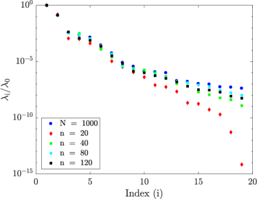
Figure 1: A comparison of the normalized eigenvalue spectrum, ($\lambda_{i}/\lambda_{0})$ using $n$ = $\{20,40,80,120\}$ samples with that obtained using a much larger sample size, $N$ = 1000.

We observe that the dominant eigenvalues, $\lambda_{1},\ldots,\lambda_{4}$, are approximated reasonably well with just 20 samples. As expected, the accuracy of higher-index eigenvalues is observed to improve with the sample size. Since $\lambda_{1}$ is roughly an order of magnitude larger than $\lambda_{2}$, we expect a 1-dimensional active subspace to reasonably approximate the uncertainty in the ignition delay. To further confirm this, we evaluate a relative L² norm of the difference ($\varepsilon_{\text{L}^{2}}^{N-n}$) between the squared value of corresponding components of the dominant eigenvector, computed using $N$ = 1000 (${\mathchoice{\mbox{\boldmath$\displaystyle{w}$}}{\mbox{\boldmath$\textstyle{w}$}}{\mbox{\boldmath$\scriptstyle{w}$}}{\mbox{\boldmath$\scriptscriptstyle{w}$}}}_{1,N}$) and $n$ = $\{20,40,80,120\}$ (${\mathchoice{\mbox{\boldmath$\displaystyle{w}$}}{\mbox{\boldmath$\textstyle{w}$}}{\mbox{\boldmath$\scriptstyle{w}$}}{\mbox{\boldmath$\scriptscriptstyle{w}$}}}_{1,n}$) as follows:

$$\varepsilon_{\text{L}^{2}}^{N-n}=\frac{\|{\mathchoice{\mbox{\boldmath$\displaystyle{w}$}}{\mbox{\boldmath$\textstyle{w}$}}{\mbox{\boldmath$\scriptstyle{w}$}}{\mbox{\boldmath$\scriptscriptstyle{w}$}}}_{1,N}^{2}-{\mathchoice{\mbox{\boldmath$\displaystyle{w}$}}{\mbox{\boldmath$\textstyle{w}$}}{\mbox{\boldmath$\scriptstyle{w}$}}{\mbox{\boldmath$\scriptscriptstyle{w}$}}}_{1,n}^{2}\|_{2}}{\|{\mathchoice{\mbox{\boldmath$\displaystyle{w}$}}{\mbox{\boldmath$\textstyle{w}$}}{\mbox{\boldmath$\scriptstyle{w}$}}{\mbox{\boldmath$\scriptscriptstyle{w}$}}}_{1,N}^{2}\|_{2}}$$ (12)

The quantity, $\varepsilon_{\text{L}^{2}}^{N-n}$, was found to be $\mathcal{O}(10^{-2})$ in all cases. Thus, even a small sample size, $n$ = 20, seems to approximate the dominant eigenspace with reasonable accuracy in this case. The iterative strategy therefore offers a significant potential for computational gains.

The active subspace for the 19-dimensional problem was also computed using regression-based estimates of the gradient that do not require model evaluations at neighboring points as discussed earlier. The quantity, $\max\limits_{j}(\delta\hat{\mathbf{{W}}}_{1,j}^{(r)})$ defined in Algorithm 4 was used to assess the convergence behavior of the two approaches. Using a set tolerance, $\tau$ = 0.05, it was observed that both perturbation and regression approaches took 8 iterations to converge. Note that the computational effort at each iteration was considered to be the same in both cases. More specifically, 5 new random samples were added for the perturbation approach at each iteration. However, as discussed earlier, a total of 100 (=5$\times$(19+1)) model runs were needed to obtain the model prediction and its gradients at these newly generated samples. Hence, in the case of regression, 100 new random samples were generated at each iteration since gradient computation does not require additional model runs in this case. Thus, including the initial step, a total of 900 model runs were required to obtain a converged active subspace in both cases.

The accuracy of the two approaches was assessed by estimating $\varepsilon_{\text{L}^{2}}^{N-n}$ using the components of the dominant eigenvector in the converged active subspace in each case in (12). The quantity, $\varepsilon_{\text{L}^{2}}^{N-n}$ was estimated to be 0.0657 and 0.1050 using perturbation and regression respectively. Hence, the regression approach was found to be relatively more accurate. Squared values of the individual components of the dominant eigenvector from the two approaches and for the case using $N$ = 1000 in the perturbation approach are plotted in Figure 2 (left).

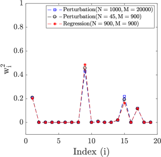
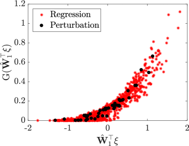
Figure 2: Left: An illustrative comparison of individual squared components of the converged dominant eigenvector obtained using perturbation and regression strategies using $M$ = 900 model runs in each case. Additionally, the dominant eigenvector components obtained using $M$ = 20000 model runs (corresponding to $N$ = 1000 samples) in the perturbation strategy (test case), used to assess the accuracy of the two strategies are also plotted. Right: An illustrative comparison of the SSPs generated using the perturbation and the regression strategies for computing the active subspace.

The set of eigenvector components for the three cases are found to be in excellent agreement with each other, indicating that both approaches have sufficiently converged and are reasonably accurate for this setup.

As mentioned earlier, the model output $f(\bm{\xi})$ i.e. the ignition delay in the H₂/O₂ reaction in this case, varies predominantly in a 1-dimensional active subspace. Hence, $f(\bm{\xi})$ can be approximated as $G(\hat{\mathbf{{W}}}_{1}^{\top}\bm{\xi})$ in the 1-dimensional active subspace. The plot of $G$ versus $\hat{\mathbf{{W}}}_{1}^{\top}\bm{\xi}$, regarded as the sufficient summary plot (SSP), obtained using the perturbation-based and regression-based gradient estimates are compared in Figure 2 (right). The dominant eigenvector obtained using perturbation is based on $N$ = 45 samples which requires $M$ = 900 model runs. For the same amount of computational effort, we can afford $N$ = 900 samples when using regression. Hence, the SSP from regression is based on 900 points: ($\hat{\mathbf{{W}}}_{1}^{\top}\bm{\xi}_{j}$, $G(\hat{\mathbf{{W}}}_{1}^{\top}\bm{\xi}_{j})$), $j=1,\ldots,900$. On the other hand, the SSP from perturbation is plotted using only 45 points as mentioned earlier. Nevertheless, the illustrative comparison clearly indicates that the two SSPs are in excellent agreement. Moreover, it is interesting to note that the response in ignition delay based on the considered probability distributions for $\log(A_{i})$ although non-linear, can be approximated by a 1-dimensional active subspace.

We further estimate the normalized activity scores for individual uncertain inputs ($\tilde{\nu}_{i,r}$; $r$=1 since a 1-dimensional active subspace seems reasonably accurate) using the components of the dominant eigenvector as shown in Algorithm 4 (steps 21 and 22). The activity scores for the 19 uncertain pre-exponents ($A_{i}$’s), estimated using the perturbation and regression strategies are plotted in Figure 3.

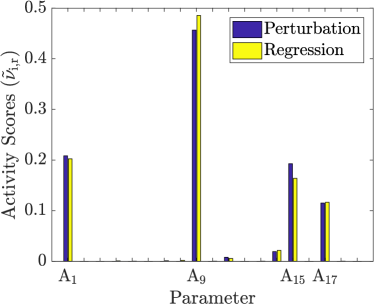
Figure 3: Left: A bar-graph of normalized activity scores ($\tilde{\nu}_{i,r}$’s) for the 19 uncertain pre-exponents ($A_{i}$’s); $r$ denotes the number of eigenvectors in the dominant eigenspace.

The activity scores based on the two approaches for gradient estimation agree favorably with each other as well as those based on the screening metric involving the DGSMs in [40]. It is observed that the uncertainty associated with the ignition delay is largely due to the uncertainty in $A_{9}$ while $A_{1}$, $A_{15}$, and $A_{17}$ are also observed to contribute significantly towards its variance.

The above comparisons indicate that the gradient of the ignition delay with respect to the uncertain $A_{i}$’s is reasonably approximated using both, perturbation and regression approaches in this case. Since both approaches yield consistent results and are comparable in terms of convergence and accuracy, we could use either for the purpose of active subspace computation for this setting. In the following section, we shift our focus to the higher-dimensional H₂/O₂ reaction kinetics application wherein the activation energies in the rate law as well as initial pressure, temperature, and stoichiometric conditions are also considered to be uncertain.

5 $\text{H}_{2}$/$\text{O}_{2}$ reaction kinetics: higher-dimensional case

For the high-dimensional case, we aim to investigate the impact of uncertainty in the following problem parameters on the ignition delay associated with the H₂/O₂ reaction: (i) pre-exponents ($A_{i}$’s); (ii) the activation energies ($E_{a,i}$’s); and (iii) the initial pressure ($P_{0}$), temperature ($T_{0}$), and stoichiometry ($\Phi_{0}$). The $\log(A_{i})$’s, $E_{a,i}$’s for all reactions except $\mathcal{R}_{6}$ – $\mathcal{R}_{9}$, $\mathcal{R}_{13}$ (due to zero nominal values for $E_{a}$), and the initial conditions were considered to be uniformly distributed, and perturbed by 2$\%$ about their nominal values. Note that the magnitude of the perturbation was selected such that the ignition delay assumes a physically meaningful value in the input domain. The nominal values of the rate parameters, $A_{i}$’s and $E_{a,i}$’s were taken from [18]. The nominal values of $P_{0}$, $T_{0}$, and $\Phi_{0}$ were considered to be 1.0 atm, 900 K, and 2.0 respectively.

5.1 Computing the active subspace

The active subspace was computed using the iterative procedure outlined in Algorithm 4. The convergence of the eigenvectors was examined by tracking the quantity ‘$\max\limits_{j}(\delta\hat{\mathbf{{W}}}_{1,j}^{(i)})$’. In Figure 4 (right), we examine $\max\limits_{j}(\delta\hat{\mathbf{{W}}}_{1,j}^{(i)})$ with increasing iterations for the perturbation and the regression approaches discussed earlier in Section 4.

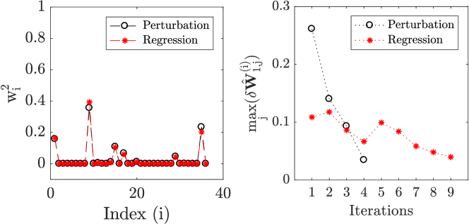
Figure 4: Left: An illustrative comparison of individual components of the dominant eigenvector in the converged active subspace i.e., at the end of 4 iterations in the perturbation approach and 9 iterations in the regression approach. Right: A comparison of the convergence behavior of the perturbation and the regression approaches. Convergence is accomplished once $\max\limits_{j}(\delta\hat{\mathbf{{W}}}_{1,j}^{(i)})$ assumes a value smaller than 0.05.

At each iteration, we improve our estimates of the matrix $\hat{\mathbf{{C}}}$ by estimating the gradient of the ignition delay at 5 new randomly generated samples in the 36-dimensional input space. However, gradient computation at these 5 samples requires 185 (=5$\times$(36+1)) model runs when using perturbation. For the same computational effort, the regression approach can afford 185 new samples at each iteration. It is observed that using $\tau$ = 0.05, the active subspace requires 4 iterations (925 model runs) to converge in the case of perturbation, and 9 iterations (1850 model runs) to converge in the case of regression. Hence, the computational effort required to obtain a converged active subspace is doubled when using regression to approximate the gradient. Moreover, gradient estimation in the perturbation approach can be made more efficient by using techniques such as automatic differentiation [42] and adjoint computation [23]. These techniques although not pursued here are promising directions for future efforts pertaining to this work. In Figure 4 (right), we compare individual components of the dominant eigenvector in the converged active subspace obtained using the two approaches. The components are observed to be in excellent agreement with each other.

In Figure 5, we plot the SSP for the perturbation approach (left) and the regression approach (center) in a 1-dimensional active subspace. A 1-dimensional polynomial fit is also illustrated in both cases. Moreover, the two surrogates are shown to be consistent with each other (right). From these results, it is clear that a 1-dimensional active subspace captures the variability in the ignition delay with reasonable accuracy, and that the two approaches yield consistent results.

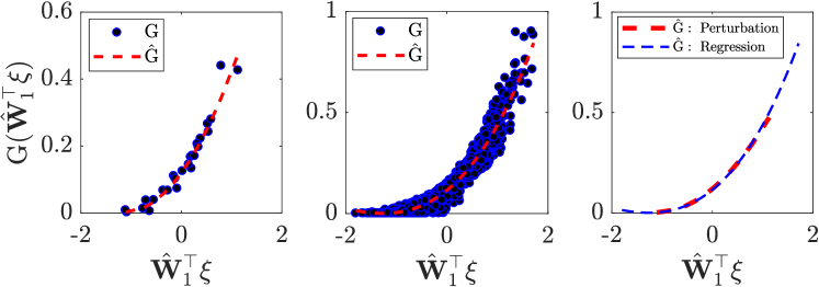
Figure 5: Sufficient summary plots (SSPs) for the case of perturbation (left) and regression (center). A polynomial fit of degree 2 and 3 as shown in the plots is used as a surrogate in the perturbation and regression approaches respectively. An illustrative comparison of the two surrogates is also provided (right).

5.2 Surrogate Assessment

The 1-dimensional surrogate ($\hat{G}$) shown in Figure 5 for the perturbation and regression approaches is investigated for its ability to capture the uncertainty in the ignition delay. Specifically, we compare probability density functions (PDFs) obtained using the true set of model evaluations, and 1-dimensional surrogates ($\hat{G}$’s) based on the two approaches, as shown in Figure 6. Note that the three PDFs were evaluated using the same set of 10⁴ samples in the cross-validation set.

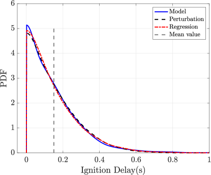
Figure 6: A comparison of the PDFs of ignition delay, obtained using model evaluations (solid line) and 1-dimensional surrogates using the regression-based strategy (dashed line) and the perturbation-based strategy (dashed-dotted line). The same set of 10⁴ samples in the cross-validation set were used in each case.

The PDFs are observed to be in close agreement with each other. Specifically, the modal estimate and the uncertainty (quantified by the spread in the distributions) is found to be consistent for the three cases. To confirm this, we further compute the first-order (mean) and the second-order (standard deviation) statistics of the estimates of the ignition delay obtained using the model, 1-dimensional surrogate from perturbation, and 1-dimensional surrogate from regression at the cross-validation sample set. The mean and standard deviation estimates are provided in Table 2.

Distribution	$\mu$	$\sigma$
$G$ (Model)	0.15	0.14
$\hat{G}$ (Perturbation-based)	0.15	0.13
$\hat{G}$ (Regression-based)	0.15	0.13

Table 2: The mean ($\mu$), and the standard deviation ($\sigma$), computed using the model ($G$), and the surrogate ($\hat{G}$) based on the two strategies at 10⁴ samples in the cross-validation set.

The mean and the standard deviation estimates obtained using the model and the 1-dimensional surrogates are found to be in close agreement. Hence, the uncertainty in the ignition delay is accurately captured in both cases.

5.3 GSA consistency check

The normalized activity scores ($\tilde{\nu}_{i,r}$) based on the 1-dimensional active subspace, obtained using the two approaches for gradient estimation (perturbation and regression), are compared with the total-effect Sobol’ indices in Figure 7. Note that the Sobol’ indices were computed using the verified 1-dimensional surrogate ($\hat{G}$) in the active subspace, obtained using the perturbation approach.

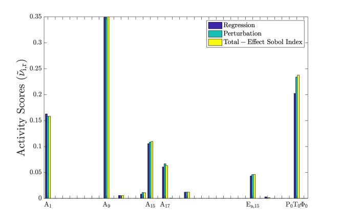
Figure 7: Bar graphs illustrating individual activity scores for the uncertain rate parameters and the initial conditions for the H₂/O₂ reaction.

Several useful inferences can be drawn. Firstly, the normalized activity scores from the two approaches and the total-effect Sobol’ indices are found to be in close agreement with each other. Secondly, as expected, $\tilde{\nu}_{i,r}$ based on perturbation exhibits a better agreement with the total-effect Sobol’ indices since the 1-dimensional surrogate based on the same approach was used to evaluate the Sobol’ indices. This observation demonstrates that the proposed framework is self-consistent. Thirdly, the variability in the ignition delay is predominantly due to the uncertainty in $A_{1}$, $A_{9}$, and $T_{0}$ while contributions from the uncertainty in $A_{15}$, $A_{17}$, and $E_{a,15}$, and $T_{0}$ are also found to be significant. The remaining rate parameters, initial pressure ($P_{0}$), and stoichiometry ($\Phi_{0}$) do not seem to impact the ignition delay in their considered intervals. Therefore, GSA has helped identify the important rate parameters i.e. key contributors to the uncertainty, and also demonstrated that among the considered uncertain initial conditions, the ignition delay is mainly impacted by the perturbations in the initial temperature in the considered interval.

As shown in the PDF plotted in Figure 6, the ignition delay assumes a wide range of values, i.e. from about 2 ms to 400 ms. However, for many practical applications, a much smaller ignition delay (0.1 ms–1 ms) might be of interest. The authors would like to point out that the proposed framework was also implemented to such a regime by using a nominal value of the initial temperature, $T_{0}$ = 1000 K, and the initial pressure, $P_{0}$ = 1.5 atm. Our analysis for this regime once again revealed that a 1-dimensional active subspace was able to capture the variability in the ignition delay due to the uncertainty in the rate-controlling parameters and the input conditions. The sensitivity trends were also found to be qualitatively similar to those presented in Figure 7. We have not included these results in the interest of brevity. Therefore, the proposed methodology was tested for is robustness and applicability for a wide range of conditions pertaining to the considered application.

6 Summary and Discussion

In this work, we focused on the uncertainty associated with the rate-controlling parameters in the H₂/O₂ reaction mechanism as well as the initial pressure, temperature, and stoichiometry and its impact on ignition delay predictions. The mechanism involves 19 different reactions and in each case, the reaction rate depends upon the choice of a pre-exponent and an activation energy. Hence, in theory, the evolution of the chemical system depends upon 38 rate parameters and three initial conditions. However, we considered epistemic uncertainty in all pre-exponents and activation energies with non-zero nominal values i.e. a total of 33 rate parameters instead of 38 in addition to the three initial conditions. To facilitate efficient uncertainty analysis, we focused our efforts on reducing the dimensionality of the problem by identifying important directions in the parameter space such that the model output predominantly varies along these directions. These important directions constitute the active subspace. Additionally, we demonstrated that the activity scores, computed using the components of the dominant eigenvectors provide an efficient means for approximating derivative based global sensitivity measures (DGSMs). Furthermore, we established generalized mathematical linkages between the different global sensitivity measures: activity scores, DGSMs, and total Sobol’ index which could be exploited to reduce computational effort associated with global sensitivity analysis.

Active subspace computation requires repeated evaluations of the gradient of the QoI i.e. the ignition delay. For this purpose, we explored two approaches, namely, perturbation and regression. Both approaches were shown to yield consistent results for the 19-dimensional problem wherein only the pre-exponents were considered to be uncertain. It was observed that the computational effort required to obtain a converged active subspace was comparable for the two approaches. However, the predictive accuracy of the perturbation approach was found to be relatively higher. Moreover, a 1-dimensional active subspace was shown to reasonably approximate the uncertainty in the ignition delay. Additionally, the activity scores were also shown to be consistent with the screening metric estimates based on DGSMs in [40]. An iterative procedure was adopted to enhance the computational efficiency.

The active subspace was further computed for a 36-dimensional problem wherein all pre-exponents and activation energies with non-zero nominal estimates as well as the initial conditions were considered uncertain. Once again, consistent results were obtained using the two approaches. A 1-dimensional active subspace was shown to reasonably capture the uncertainty in the ignition delay in this case. However, the computational effort required to compute a converged active subspace using perturbation was found to be half of the effort required in the case of regression. Predictive accuracy of the two approaches was found to be comparable. Hence, perturbation seems like a preferred approach for the higher-dimensional problem based on our findings. GSA results indicated that the variability in the ignition delay is predominantly due to the uncertainty in the rate parameters, $A_{1}$ and $A_{9}$ with significant contributions from $A_{15}$, $A_{17}$, and $E_{a,15}$. Additionally, the ignition delay was found to be sensitive towards $T_{0}$.

Based on our findings, the perturbation approach is preferable for active subspace computation; the computational cost of this approach can be reduced significantly, if more efficient gradient computation techniques (e.g., adjoint-based approaches or automatic differentiation) are feasible. The regression-based approach can be explored in situations involving intensive simulations where gradient computation is very challenging.

We also mention that alternate regression-based approaches such as ones based on computing a global quadratic model have been proposed and used in the literature; see e.g., [43]. The applicability of such an approach in the context of high-dimensional chemical reaction networks is subject to future work.

The computational framework presented in this work is agnostic to the choice of the chemical system and can be easily adapted for other systems as long as the quantity of interest is continuously differentiable in the considered domain of the inputs. We have demonstrated that the active subspace could be exploited for efficient forward propagation of the uncertainty from inputs to the output. The resulting activity scores and the low-dimensional surrogate could further guide optimal allocation of computational resources for calibration of the important rate-controlling parameters and input conditions in a Bayesian setting. Additionally, dimension reduction using active subspaces could assist in developing robust formulations for predicting discrepancy between simulations and measurements due to epistemic uncertainty in the model inputs.

References

- [1] A. Burnham, R. Braun, H. Gregg, A. Samoun, Comparison of methods for measuring kerogen pyrolysis rates and fitting kinetic parameters, Energy Fuels 1 (1987) 452–458.
- [2] A. Burnham, R. Braun, A. Samoun, Further comparison of methods for measuring kerogen pyrolysis rates and fitting kinetic parameters, Org. Geochem. 13 (1988) 839–845.
- [3] M. Vohra, M. Grapes, P. Swaminathan, T. Weihs, O. Knio, Modeling and quantitative nanocalorimetric analysis to assess interdiffusion in a Ni/Al bilayer, J. Appl. Phys. 110 (2011) 123521.
- [4] S. Sarathy, S. Vranckx, K. Yasunaga, M. Mehl, P. Oßwald, W. Metcalfe, C. Westbrook, W. Pitz, K. Kohse-Höinghaus, R. Fernandes, et al., A comprehensive chemical kinetic combustion model for the four butanol isomers, Combust. Flame 159 (2012) 2028–2055.
- [5] M. Vohra, J. Winokur, K. Overdeep, P. Marcello, T. Weihs, O. Knio, Development of a reduced model of formation reactions in Zr-Al nanolaminates, J. Appl. Phys. 116 (2014) 233501.
- [6] M. Vohra, X. Huan, T. Weihs, O. Knio, Design analysis for optimal calibration of diffusivity in reactive multilayers, Combust. Theor. Model. 21 (2017) 1023–1049.
- [7] R. Morrison, T. Oliver, R. Moser, Representing model inadequacy: A stochastic operator approach, SIAM/ASA J. Uncertainty Quantif. 6 (2018) 457–496.
- [8] M. Hantouche, S. Sarathy, O. Knio, Global sensitivity analysis of n-butanol reaction kinetics using rate rules, Combust. Flame 196 (2018) 452–465.
- [9] S. Nannapaneni, S. Mahadevan, Reliability analysis under epistemic uncertainty, Reliab. Eng. Syst. Saf. 155 (2016) 9–20.
- [10] S. Sankararaman, S. Mahadevan, Integration of model verification, validation, and calibration for uncertainty quantification in engineering systems, Reliab. Eng. Syst. Saf. 138 (2015) 194–209.
- [11] M. Reagana, H. Najm, R. Ghanem, O. Knio, Uncertainty quantification in reacting-flow simulations through non-intrusive spectral projection, Combust. Flame 132 (2003) 545–555.
- [12] P. Constantine, Active Subspaces: Emerging Ideas for Dimension Reduction in Parameter Studies, Vol. 2, SIAM, Philadelphia, PA, USA, 2015.
- [13] S. Lam, Singular perturbation for stiff equations using numerical methods, in: Recent advances in the aerospace sciences, Springer, 1985, pp. 3–19.
- [14] S. Lam, D. Goussis, Understanding complex chemical kinetics with computational singular perturbation, in: Symposium (International) on Combustion, Vol. 22, Elsevier, 1989, pp. 931–941.
- [15] M. Valorani, F. Creta, D. Goussis, J. Lee, H. Najm, An automatic procedure for the simplification of chemical kinetic mechanisms based on CSP, Combust. Flame 146 (1) (2006) 29–51.
- [16] B. Debusschere, Y. Marzouk, H. Najm, B. Rhoads, D. Goussis, M. Valorani, Computational singular perturbation with non-parametric tabulation of slow manifolds for time integration of stiff chemical kinetics, Combust. Theor. Model. 16 (1) (2012) 173–198.
- [17] M. Salloum, A. Alexanderian, O. Le Maître, H. Najm, O. Knio, Simplified CSP analysis of a stiff stochastic ODE system, Comput. Methods Appl. Mech. Eng. 217–220 (2012) 121–138.
- [18] R. Yetter, F. Dryer, H. Rabitz, A comprehensive reaction mechanism for carbon monoxide/hydrogen/oxygen kinetics, Combust. Sci. Technol. 79 (1991) 97–128.
- [19] L. Das, Hydrogen-oxygen reaction mechanism and its implication to hydrogen engine combustion, Int. J. Hydrogen Energy 21 (1996) 703–715.
- [20] B. Loges, A. Boddien, H. Junge, M. Beller, Controlled generation of hydrogen from formic acid amine adducts at room temperature and application in H2/O2 fuel cells, Angew. Chem. Int. Ed. 47 (2008) 3962–3965.
- [21] S. Cosnier, A. Gross, A. Le Goff, M. Holzinger, Recent advances on enzymatic glucose/oxygen and hydrogen/oxygen biofuel cells: Achievements and limitations, J. Power Sources 325 (2016) 252–263.
- [22] C. Safta, H. Najm, O. Knio, TChem-a software toolkit for the analysis of complex kinetic models, Report No. SAND2011-3282, Sandia National Laboratories, CA, USA, 2011.
- [23] A. Jameson, Aerodynamic design via control theory, J. Sci. Comput. 3 (1988) 233–260.
- [24] A. Borzì, V. Schulz, Computational optimization of systems governed by partial differential equations, SIAM, Philadelphia, PA, USA, 2011.
- [25] A. Alexanderian, N. Petra, G. Stadler, O. Ghattas, Mean-variance risk-averse optimal control of systems governed by PDEs with random parameter fields using quadratic approximations, SIAM/ASA J. Uncertainty Quantif. 5 (2017) 1166–1192.
- [26] I. Sobol, Global sensitivity indices for nonlinear mathematical models and their monte carlo estimates, Math. Comput. Simul. 55 (2001) 271–280.
- [27] B. Sudret, Global sensitivity analysis using polynomial chaos expansions, Reliab. Eng. Syst. Saf. 93 (2008) 964–979.
- [28] E. Plischke, E. Borgonovo, C. Smith, Global sensitivity measures from given data, Eur. J. Oper. Res. 226 (2013) 536–550.
- [29] J.-Y. Tissot, C. Prieur, A randomized orthogonal array-based procedure for the estimation of first-and second-order sobol’indices, J. Stat. Comput. Simul. 85 (2015) 1358–1381.
- [30] C. Li, S. Mahadevan, An efficient modularized sample-based method to estimate the first-order sobol index, Reliab. Eng. Syst. Saf. 153 (2016) 110–121.
- [31] I. Sobol’, S. Kucherenko, Derivative based global sensitivity measures and the link with global sensitivity indices, Math. Comput. Simul. 79 (2009) 3009–30017.
- [32] M. Lamboni, B. Iooss, A.-L. Popelin, F. Gamboa, Derivative-based global sensitivity measures: General links with sobol’ indices and numerical tests, Math. Comput. Simul. 87 (2013) 45–54.
- [33] P. Diaz, Global sensitivity metrics from active subspaces with applications, Master’s thesis, Colorado School of Mines (2016).
- [34] P. Constantine, P. Diaz, Global sensitivity metrics from active subspaces, Reliab. Eng. Syst. Saf. 162 (2017) 1–13.
- [35] A. Saltelli, P. Annoni, I. Azzini, F. Campolongo, M. Ratto, S. Tarantola, Variance based sensitivity analysis of model output. design and estimator for the total sensitivity index, Comput. Phys. Commun. 181 (2010) 259–270.
- [36] E. Borgonovo, A new uncertainty importance measure, Reliab. Eng. Syst. Saf. 92 (2007) 771–784.
- [37] G. Li, H. Rabitz, P. Yelvington, O. Oluwole, F. Bacon, C. Kolb, J. Schoendorf, Global sensitivity analysis for systems with independent and/or correlated inputs, J. Phys. Chem. A 114 (2010) 6022–6032.
- [38] J. Jacques, C. Lavergne, N. Devictor, Sensitivity analysis in presence of model uncertainty and correlated inputs, Reliab. Eng. Syst. Saf. 91 (2006) 1126–1134.
- [39] C. Xu, G. Gertner, Extending a global sensitivity analysis technique to models with correlated parameters, Comput. Stat. Data Anal. 51 (2007) 5579–5590.
- [40] M. Vohra, A. Alexanderian, C. Safta, S. Mahadevan, Sensitivity-driven adaptive construction of reduced-space surrogates, J Sci. Comput. (article in press).
- [41] I. Sobol’, S. Tarantola, D. Gatelli, S. Kucherenko, W. Mauntz, Estimating the approximation error when fixing unessential factors in global sensitivity analysis, Reliab. Eng. Syst. Saf. 92 (2007) 957–960.
- [42] A. Kiparissides, S. Kucherenko, A. Mantalaris, E. Pistikopoulos, Global sensitivity analysis challenges in biological systems modeling, Ind. Eng. Chem. Res. 48 (2009) 7168–7180.
- [43] P. Constantine, A. Doostan, Time-dependent global sensitivity analysis with active subspaces for a lithium ion battery model, Stat. Anal. Data Min. 10 (2017) 243–262.