Handling Nominals and Inverse Roles using Algebraic Reasoning

Abstract

This paper presents a novel $\mathcal{SHOI}$ tableau calculus which incorporates algebraic reasoning for deciding ontology consistency. Numerical restrictions imposed by nominals, existential and universal restrictions are encoded into a set of linear inequalities. Column generation and branch-and-price algorithms are used to solve these inequalities. Our preliminary experiments indicate that this calculus performs better on $\mathcal{SHOI}$ ontologies than standard tableau methods.

1 Introduction and Motivation

Description Logic (DL) is a formal knowledge representation language that is used for modeling ontologies. Modern description logic systems provide reasoning services that can automatically infer implicit knowledge from explicitly expressed knowledge. Designing reasoning algorithms with high performance has been one of the main concerns of DL researchers. One of the key features of many description logics is support for nominals. Nominals are special concept names that must be interpreted as singleton sets. They allow to use Abox individuals within concept descriptions. However, nominals carry implicit global numerical restrictions that increase reasoning complexity. Moreover, the interaction between nominals and inverse roles leads to the loss of the tree model property. Most state-of-the-art reasoners, such as Konclude [26], Fact++ [27], HermiT [24], have implemented traditional tableau algorithms. Konclude also incorporated consequence-based reasoning into its tableau calculus [25]. These reasoners try to construct completion graphs in a highly non-deterministic way in order to handle nominals. For example, a small $\mathcal{ALCO}$ ontology models Canada consisting of its ten provinces: $\mathit{CA\_Province}\equiv\{\mathit{Ontario}$, $\mathit{Quebec}$, $\mathit{NovaScotia}$, $\mathit{NewBrunswick}$, $\mathit{Manitoba}$, $\mathit{BritishColumbia}$, $\mathit{PrinceEdwardIsland}$, $\mathit{Saskatchewan}$, $\mathit{NewfoundlandAndLabrador}$, $\mathit{Alberta}\}$. If one tries to model that Canada consists of 11 provinces, it is trivial to see that it is not possible because the cardinality of $\mathit{CA\_Province}$ is implicitly restricted to the 10 provinces listed as nominals. However, according to our preliminary experiments, above mentioned DL reasoners are unable to decide this inconsistency within a reasonable amount of time. Consequence-based (CB) reasoning algorithms are also extended to more expressive DLs such as $\mathcal{SHOI}$ [6] and $\mathcal{SROI}Q$ [7]. Since their implementations are not available, we could not analyze these reasoners.

However, algebraic DL reasoners are considered more efficient in handling numerical restrictions [11, 13, 14, 28]. RacerPro [14] was the first highly optimized reasoner that combined tableau-based reasoning with algebraic reasoning [15]. Other tableau-based algebraic reasoner for $\mathcal{SHQ}$ [13], $\mathcal{SHIQ}$ [23], $\mathcal{SHOQ}$ [12, 11] are also proposed to handle qualified number restrictions (QNRs) and their interaction with inverse roles or nominals. These reasoners use an atomic decomposition technique to encode number restrictions into a set of linear inequalities. These inequalities are then solved by integer linear programming (ILP). These reasoners perform very efficiently in handling huge values in number restrictions. However, their ILP algorithms are best-case exponential to the number of inequalities. For example, in case of $m$ inequalities they require $2^{m}$ variables in order to find the optimal solution. However, for ILP with a huge number of variables it is not feasible to enumerate all variables. To overcome this problem, the column generation technique has been used [28, 30] which considers a small subset of variables. However, to the best of our knowledge, no algebraic calculus can handle DLs supporting nominals and inverse roles simultaneously.

In this paper, we present a novel algebraic tableau calculus for $\mathcal{SHOI}$ to handle a large number of nominals and their interaction with inverse roles. The rest of this paper is structured as follows. Section 2 defines important terms and introduces $\mathcal{SHOI}$. Section 3 presents the algebraic tableau calculus for $\mathcal{SHOI}$. Section 4 provides evaluation results for the implemented prototype Cicada. The last section concludes our paper.

2 Preliminaries

In this section, we introduce $\mathcal{SHOI}$ and some notations used later. Let $N=N_{C}\cup N_{o}$ where $N_{C}$ represents concept names and $N_{o}$ nominals. Let $N_{R}$ be a set of role names with a set of transitive roles $N_{R_{+}}\subseteq N_{R}$. The set of roles in $\mathcal{SHOI}$ is $N_{R}\cup\{R^{-}\mid R\in N_{R}\}$ where $R^{-}$ is called the inverse of $R$. A function $\mathsf{Inv}$ returns the inverse of a role such that $\mathsf{Inv}(R)=R^{-}$ if $R\in N_{R}$ and $\mathsf{Inv}(R)=S$ if $R=S^{-}$ and $S\in N_{R}$. An interpretation $\mathcal{I}=(\Delta^{\mathcal{I}},\cdot^{\mathcal{I}})$ consists of a non-empty set $\Delta^{\mathcal{I}}$ of individuals called the domain of interpretation and an interpretation function $\cdot^{\mathcal{I}}$. Table 1 presents syntax and semantic of $\mathcal{SHOI}$. We use $\top$ ($\bot$) as an abbreviation for $A\sqcup\neg A$ ($A\sqcap\neg A$) for some $A\in N_{C}$. In the following $\sharp\{.\}$ denotes set cardinality.

Table 1: Syntax and semantics of $\mathcal{SHOI}$

Construct	Syntax	Semantics
atomic concept	$A$	$A^{\mathcal{I}}\subseteq\Delta^{\mathcal{I}}$
negation	$\neg C$	$\Delta^{\mathcal{I}}\setminus C^{\mathcal{I}}$
conjunction	$C\sqcap D$	$C^{\mathcal{I}}\cap D^{\mathcal{I}}$
disjunction	$C\sqcup D$	$C^{\mathcal{I}}\cup D^{\mathcal{I}}$
value restriction	$\forall R.C$	$\{x\in\Delta^{\mathcal{I}}\mid\forall y:(x,y)\in R^{\mathcal{I}}\Rightarrow y\in C^{\mathcal{I}}\}$
exists restriction	$\exists R.C$	$\{x\in\Delta^{\mathcal{I}}\mid\exists y\in\Delta^{\mathcal{I}}:(x,y)\in R^{\mathcal{I}}\wedge y\in C^{\mathcal{I}}\}$
nominal	$\{o\}$	$\sharp\{o\}^{\mathcal{I}}=1$
role	$R$	$R^{\mathcal{I}}\subseteq\Delta^{\mathcal{I}}\times\Delta^{\mathcal{I}}$
inverse role	$R^{-}$	$(R^{-})^{\mathcal{I}}=\{(y,x)\mid(x,y)\in R^{\mathcal{I}}\}$
transitive role	$R\in N_{R_{+}}$	$(x,y)\in R^{\mathcal{I}}\wedge(y,z)\in R^{\mathcal{I}}\Rightarrow(x,z)\in R^{\mathcal{I}}$

A role inclusion axiom (RIA) of the form $R\sqsubseteq S$ is satisfied by $\mathcal{I}$ if $R^{\mathcal{I}}\subseteq S^{\mathcal{I}}$. We denote with $\sqsubseteq_{*}$ the transitive, reflexive closure of $\sqsubseteq$ over $N_{R}$. If $R\sqsubseteq_{*}S$, we call $R$ a subrole of $S$ and $S$ a superrole of $R$. A general concept inclusion (GCI) $C\sqsubseteq D$ is satisfied by $\mathcal{I}$ if $C^{\mathcal{I}}\subseteq D^{\mathcal{I}}$. A role hierarchy $\mathcal{R}$ is a finite set of RIAs. A Tbox $\mathcal{T}$ is a finite set of GCIs. A Tbox $\mathcal{T}$ and its associated role hierarchy $\mathcal{R}$ is satisfied by $\mathcal{I}$ (or consistent) if each GCI and RIA is satisfied by $\mathcal{I}$. Such an interpretation $\mathcal{I}$ is then called a model of $\mathcal{T}$. A concept description $C$ is said to be satisfiable by $\mathcal{I}$ iff $C^{\mathcal{I}}\neq\emptyset$. An Abox $\mathcal{A}$ is a finite set of assertions of the form ${a\!:C}$ (concept assertion) with $a^{\mathcal{I}}\in C^{\mathcal{I}}$, and ${(a,b)\!:R}$ (role assertion) with $(a^{\mathcal{I}},b^{\mathcal{I}})\in R^{\mathcal{I}}$. Due to nominals, a concept assertion ${a\!:C}$ can be transformed into a concept inclusion $\{a\}\sqsubseteq C$ and a role assertion ${(a,b)\!:R}$ into $\{a\}\sqsubseteq\exists R.\{b\}$. Therefore, concept satisfiability and Abox consistency can be reduced to Tbox consistency by using nominals. We use $\{o_{1},\ldots,o_{n}\}$ as an abbreviation for $\{o_{1}\}\sqcup\cdots\sqcup\{o_{n}\}$ and may write $\{o\}$ as $o$. Moreover, we do not make the unique name assumption; therefore, two nominals might refer to the same individual.

Nominals carry implicit global numerical restrictions. For example, if $C\sqsubseteq\{o_{1},o_{2},o_{3}\}$ (or $\{o_{1},o_{2},o_{3}\}\sqsubseteq C$), then $o_{1},o_{2},o_{3}$ impose a numerical restriction that there can be at most (or at least, if $o_{1},o_{2},o_{3}\in N_{o}$ are declared as pair-wise disjoint) three instances of $C$. These restrictions are global because they affect the set of all individuals of $C$ in $\Delta^{\mathcal{I}}$. These implicit numerical restrictions increase reasoning complexity.

3 An Algebraic Tableau Calculus for $\mathcal{SHOI}$

In this section, we present an algebraic tableau calculus for $\mathcal{SHOI}$ that decides Tbox consistency. Since nominals carry numerical restrictions, algebraic reasoning is used to ensure their semantics. The algorithm takes a $\mathcal{SHOI}$ Tbox $\mathcal{T}$ and its role hierarchy $\mathcal{R}$ as input and tries to create a complete and clash-free completion graph in order to check Tbox consistency. The reasoner is divided into two modules: 1) Tableau Module (TM), and 2) Algebraic Module (AM).

Let $G=(V,E,\mathcal{L},\mathcal{B})$ be a completion graph for a $\mathcal{SHOI}$ Tbox $\mathcal{T}$ where $V$ is a set of nodes and $E$ a set of edges. Each node $x\in V$ is labelled with a set of concepts $\mathcal{L}(x)$, and each edge $\left\langle x,y\right\rangle\in E$ with a set of role names $\mathcal{L}(x,y)$. For each node $x\in V$, if $\mathcal{L}(x)$ contains a universal restriction on role $R$ and there exists an $R$-neighbour of $x$, then $\mathcal{B}(x)$ contains a tuple of the form $\left\langle v,\mathcal{L}(x,v)\right\rangle$ where $v\in V$ is an $R$-neighbour of $x$. We use $\sharp v$ to denote the cardinality of a node $v$. For convenience, we assume that all concept descriptions are in negation normal form.

TM starts with some preprocessing and reduces all the concept axioms in a Tbox $\mathcal{T}$ to a single axiom $\top\sqsubseteq C_{\mathcal{T}}$ such that $C_{\mathcal{T}}\coloneqq\bigsqcap_{C\sqsubseteq D\in\mathcal{T}}\mathit{nnf}(\neg C\sqcup D)$, where $\mathit{nnf}$ transforms a given concept expression to its negation normal form. The algorithm checks consistency of $\mathcal{T}$ by testing the satisfiability of $o\sqsubseteq C_{\mathcal{T}}$ where $o\in N_{o}$ is a fresh nominal in $\mathcal{T}$, which means that at least $o^{\mathcal{I}}\in{C_{\mathcal{T}}}^{\mathcal{I}}$ and ${C_{\mathcal{T}}}^{\mathcal{I}}\neq\emptyset$. Moreover, since ${\top^{\mathcal{I}}}={\Delta^{\mathcal{I}}}$ then every domain element must also satisfy $C_{\mathcal{T}}$. For creating a complete and clash-free completion graph, TM applies expansion rules (see Figure 1 and Section 3.1). AM handles all numerical restrictions using ILP. It generates inequalities and solves them using the branch-and-price technique (see Section 3.2 for details). We use equality blocking [18, 16] due to the presence of inverse roles.

3.1 Expansion Rules

In order to check the consistency of a Tbox $\mathcal{T}$, the proposed algorithm creates a completion graph $G$ using the expansion rules shown in Figure 1. A node $x$ in $G$ contains a clash if $\{A,\neg A\}\subseteq\mathcal{L}(x)$ for $A\in N_{C}$ or AM has no feasible solution for $x$. $G$ is complete if no expansion rule is applicable to any node in $G$. $\mathcal{T}$ is consistent if $G$ is complete and no node in $G$ contains a clash.

The $\sqcap$-Rule, $\sqcup$-Rule and $\forall$-Rule are similar to standard tableau expansion rules for $\mathcal{ALC}$. The $\forall_{+}$-Rule preserves the semantics of transitive roles. The $\mathit{nom_{\mathit{merge}}}$-Rule merges two nodes containing in their label the same nominal. Suppose there is $o\in\mathcal{L}(x)$ and $o\in\mathcal{L}(y)$, and nodes $x$ and $y$ are not the same, then $\mathit{nom_{\mathit{merge}}}$-Rule merges $x$ into $y$. It adds $\mathcal{L}(x)$ to $\mathcal{L}(y)$ and moves all edges leading to (from) $x$ so that they lead to (from) $y$. For each node $z$, if $\left\langle z,y\right\rangle\in E$ and $\left\langle z,x\right\rangle\in E$, then $\mathcal{L}(z,y)=\mathcal{L}(z,y)\cup\mathcal{L}(z,x)$. Similarly, if $\left\langle y,z\right\rangle\in E$ and $\left\langle x,z\right\rangle\in E$, then $\mathcal{L}(y,z)=\mathcal{L}(y,z)\cup\mathcal{L}(x,z)$. It also merges $\mathcal{B}(x)$ into $\mathcal{B}(y)$.

$\sqcap$-Rule	if $(C_{1}\sqcap C_{2})\in\mathcal{L}(x)$ and $\{C_{1},C_{2}\}\nsubseteq\mathcal{L}(x)$ then set $\mathcal{L}(x)=\mathcal{L}(x)\cup\{C_{1},C_{2}\}$
$\sqcup$-Rule	if $(C_{1}\sqcup C_{2})\in\mathcal{L}(x)$ and $\{C_{1},C_{2}\}\cap\mathcal{L}(x)=\emptyset$ then set $\mathcal{L}(x)=\mathcal{L}(x)\cup\{C\}$ for some $C\in\{C_{1},C_{2}\}$
$\forall$-Rule	if $\forall S.C\in\mathcal{L}(x)$ and there $\exists y$ with $R\in\mathcal{L}(x,y)$, $C\notin\mathcal{L}(y)$ and $R\sqsubseteq_{*}S$ then set $\mathcal{L}(y)=\mathcal{L}(y)\cup\{C\}$
$\forall_{+}$-Rule	if $\forall S.C\in\mathcal{L}(x)$ and there exist $U,R$ with $R\in N_{R_{+}}$ and $U\sqsubseteq_{*}R$, $R\sqsubseteq_{*}S$, and a node $y$ with $U\in\mathcal{L}(x,y)$ and $\forall R.C\notin\mathcal{L}(y)$ then set $\mathcal{L}(y)=\mathcal{L}(y)\cup\{\forall R.C\}$
$\mathit{nom_{\mathit{merge}}}$-Rule	if for some $o\in N_{o}$ there are nodes $x$, $y$ with $o\in\mathcal{L}(x)\cap\mathcal{L}(y)$, $x\neq y$ then if $x$ is an initial node, then merge $y$ into $x$, else merge $x$ into $y$
$\mathit{inverse}$-Rule	if $\forall R^{-}.C\in\mathcal{L}(y)$, $R\in\mathcal{L}(x,y)$, and $\left\langle x,\mathcal{L}(y,x)\right\rangle\notin\mathcal{B}(y)$ then set $\mathcal{B}(y)=\mathcal{B}(y)\cup\{\left\langle x,\mathcal{L}(y,x)\right\rangle\}$
$\mathit{fil}$-Rule	if $\left\langle\mathsf{R,C},n,\mathsf{V}\right\rangle\in\sigma(x)$ and $x$ is not blocked then 1. if $\mathsf{V}=\emptyset$ and there exists no $\mathsf{R}$-neighbour $y$ of $x$ with $\mathsf{C}\subseteq\mathcal{L}(y)$, $\sharp y\geq n$, then create a new node $y$ with $\mathcal{L}(y)\leftarrow\mathsf{C}$ and $\sharp y\leftarrow n$ 2. else for all $v\in\mathsf{V}$ add $\mathsf{C}$ to $\mathcal{L}(v)$ and set $\sharp v=n$
$e$-Rule	if $\left\langle\mathsf{R,C},n,\mathsf{V}\right\rangle\in\sigma(x)$ and $\mathsf{C}\subseteq\mathcal{L}(y)$, $\sharp y\geq n$, $\mathsf{R}\nsubseteq\mathcal{L}(x,y)$ then merge $\mathsf{R}$ into $\mathcal{L}(x,y)$ and $\{\mathsf{Inv}(R)\mid R\in\mathsf{R}\}$ into $\mathcal{L}(y,x)$, and for all $S$ with $R\sqsubseteq_{*}S\in\mathcal{R}$ add $S$ to $\mathcal{L}(x,y)$ and $\mathsf{Inv}(S)$ to $\mathcal{L}(y,x)$

Figure 1: The expansion rules for $\mathcal{SHOI}$

If $\mathcal{L}(x,y)=\{R\}$ and $\forall R^{-}.C\in\mathcal{L}(y)$, then the $\mathit{inverse}$-Rule encodes for AM the already existing $R^{-}$-edge by adding a tuple $\left\langle x,\{R^{-}\}\right\rangle$ to $\mathcal{B}(y)$. AM plays also an important role if nominals occur in universal restriction. For example, consider the axioms $A\sqsubseteq\exists R.B$, $B\sqsubseteq\exists R^{-}.C\sqcap\exists R^{-}.D\sqcap\forall R^{-}.\{o_{1},o_{2}\}$ and $o_{1}\sqcap o_{2}\sqsubseteq\bot$, where $A,B,C,D\in N_{C}$, $o_{1},o_{2}\in N_{o}$ and $R\in N_{R}$. Suppose we have $A\in\mathcal{L}(x)$, $R\in\mathcal{L}(x,y)$ and $B\in\mathcal{L}(y)$. Since nominals carry numerical restrictions, $\forall R^{-}.\{o_{1},o_{2}\}$ implies that we can have at most 2 $R^{-}$-neighbours of $y$. However, standard tableau reasoners might create two new $R^{-}$-neighbours of $y$ without considering the existing $R^{-}$-neighbour $x$ of $y$. Then they try to merge these three nodes in a non-deterministic way to satisfy the numerical restriction imposed by nominals. In our approach, the $\mathit{inverse}$-Rule encodes information about an existing $R^{-}$-neighbour of $y$ and AM generates a deterministic solution.

For a node $x$, AM transforms all existential restrictions, universal restrictions and nominals to a corresponding system of inequalities. AM then processes these inequalities and gives back a solution set $\sigma(x)$. The set $\sigma(x)$ is either empty or contains solutions derived from feasible inequalities. In case of infeasibility AM signals a clash. A solution is defined by a set of tuples of the form $\left\langle\mathsf{R},\mathsf{C},n,\mathsf{V}\right\rangle$ with $\mathsf{R}\subseteq N_{R}$, $\mathsf{C}\subseteq N$, $n\in\mathbb{N}$, $n\geq 1$ and $\mathsf{V}\subseteq V$. Each tuple represents $n$ $\mathsf{R}$-neighbours of $x$ (where $\mathsf{R}$ is a set of roles) that are instances of all elements of $\mathsf{C}$. Here, $\mathsf{V}$ is an optional set that contains existing $\mathsf{R}$-neighbours of $x$ that must be reused and $\mathsf{C}$ is added to their labels. Consider the axiom $A\sqsubseteq\exists R.B\sqcap\exists R.C\sqcap\forall S.\left\{o\right\}$, where $A,B,C\in N_{C}$, $o\in N_{o}$, $R,S\in N_{R}$, $R\sqsubseteq S$, and $A\in\mathcal{L}(x)$. AM returns the solution $\sigma(x)=\{\left\langle\{R,S\},\{B,C,o\},1\right\rangle\}$. The $\mathit{fil}$-Rule is used to generate nodes based on the arithmetic solution that satisfies a set of inequalities. For the above solution, the $\mathit{fil}$-Rule creates one node $y$ with cardinality 1 such that $\mathcal{L}(y)\leftarrow\{B,C,o\}$ and $\sharp y=1$. The $e$-Rule creates an edge between nodes $x$ and $y$, and adds $R,S$ to $\mathcal{L}(x,y)$ and $\mathsf{Inv}(R),\mathsf{Inv}(S)$ to $\mathcal{L}(y,x)$. The $e$-Rule always adds all implied superroles to edge labels.

3.2 Generating Inequalities

Dantzig and Wolfe [9] proposed a column generation technique for solving linear programming (LP) problems, called Dantzig–Wolfe decomposition, where a large LP is decomposed into a master problem and a subproblem (or pricing problem). In case of LP problems with a huge number of variables, column generation works with a small subset of variables and builds a Restricted Master Problem (RMP). The Pricing Problem (PP) generates a new variable with the most reduced cost if added to RMP (see [4, 29] for details). However, column generation may not necessarily give an integral solution for an LP relaxation, i.e., at least one variable has not an integer value. Therefore, the branch-and-price method [3] has been used which is a combination of column generation and branch-and-bound technique [10]. We employ this technique by mapping number restrictions to linear inequality systems using a column generation ILP formulation (see [29] for details). CPLEX [5] has been used to solve our ILP formulation.

3.2.1 Encoding Existential Restrictions and Nominals into Inequalities

The atomic decomposition technique [22] is used to encode numerical restrictions on concepts and role fillers into inequalities. These inequalities are then solved for deciding the satisfiability of the numerical restrictions. The existential restrictions are converted into $\geq 1$ inequalities. The cardinality of a partition element containing a nominal $o$ is equal to $1$ due to the nominal semantics; $\sharp\{o\}^{I}=1$ for each nominal $o\in N_{o}$. Therefore, the decomposition set is defined as $Q=Q_{\exists}\cup Q_{\forall}\cup Q_{o}$, where $Q_{\exists}$ ($Q_{\forall}$) contains existential (universal) restrictions and $Q_{o}$ contains all related nominals. Each element $R_{q}\in Q_{\exists}\cup Q_{\forall}$ represents a role $R\in N_{R}$ and its qualification concept expression $q$ and each element $I_{q}\in Q_{o}$ represents a nominal $q\in N_{o}$. The elements in $Q_{\forall}$ are used by AM to ensure the semantics of universal restrictions. The set of related nominals $Q_{o}\subseteq N_{o}$ is defined as $Q_{o}=\{o\mid o\in clos(q)\wedge R_{q}\in Q_{\exists}\cup Q_{\forall}\}$ where $clos(q)$ is the closure of concept expression $q$. The atomic decomposition considers all possible ways to decompose $Q$ into sets that are semantically pairwise disjoint.

3.2.2 Branch-and-Price Method

In the following, we use a Tbox $\mathcal{T}$ and its role hierarchy $\mathcal{R}$, a completion graph $G$, a decomposition set $Q$ and a partitioning $\mathcal{P}$ that is the power set of $Q$ containing all subsets of $Q$ except the empty set. Each partition element $p\in\mathcal{P}$ represents the intersection of its elements. We decompose our problem into two subproblems: (i) restricted master problem (RMP), and (ii) pricing problem (PP). RMP contains a subset of columns and PP computes a column that can maximally reduce the cost of RMP’s objective. Whenever a column with negative reduced cost is found, it is added to RMP. Number restrictions are represented in RMP as inequalities, with a restricted set of variables. The flowchart in Figure 2 illustrates the whole process.

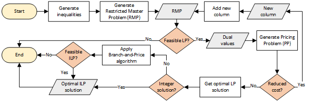
Figure 2: Overview of the algebraic reasoning process

Restricted Master Problem

RMP is obtained by considering only variables $x_{p}$ with $p\in\mathcal{P}^{\prime}$ and $\mathcal{P}^{\prime}\subseteq\mathcal{P}$ and relaxing the integrality constraints on the $x_{p}$ variables. Initially $\mathcal{P}^{\prime}$ is empty and RMP contains only artificial variables $h$ to obtain an initial feasible inequality system. Each artificial variable corresponds to an element in $Q_{\exists}\cup Q_{o}$ such that $h_{R_{q}}$, $R_{q}\in Q_{\exists}$ and $h_{I_{q}}$, $I_{q}\in Q_{o}$. An arbitrarily large cost $M$ is associated with every artificial variable. If any of these artificial variables exists in the final solution, then the problem is infeasible. The objective of RMP is defined as the sum of all costs as shown in (1) of the RMP below.

$$\text{Min}\sum_{p\in\mathcal{P}^{\prime}}cost_{p}x_{p}+M\!\!\sum_{R_{q}\in Q_{\exists}}h_{R_{q}}+M\!\!\sum_{I_{q}\in Q_{o}}h_{I_{q}}\quad\text{subject to}$$ (1)

$$\sum_{p\in\mathcal{P}^{\prime}}a_{p}^{R_{q}}x_{p}+h_{R_{q}} \geq \ 1 \quad R_{q}\in Q_{\exists}$$ (2)

$$\sum_{p\in\mathcal{P}^{\prime}}a_{p}^{I_{q}}x_{p}+h_{I_{q}} = \ 1 \quad I_{q}\in Q_{o}$$ (3)

$$x_{p}\in\mathbb{R}^{+}\text{ with }p\in\mathcal{P}^{\prime}$$ (4)

$$a_{p}^{R_{q}},a_{p}^{I_{q}}\in\{0,1\},\,h_{R_{q}},h_{I_{q}}\in\mathbb{R}^{+}\text{ with }R_{q}\in Q_{\exists},\,I_{q}\in Q_{o}$$

where a decision variable $x_{p}$ represents the elements of the partition element $p\in\mathcal{P}^{\prime}$. The coefficients $a_{p}$ are associated with variables $x_{p}$ and $a_{p}^{R_{q}}$ indicates whether an $R$-neighbour that is an instance of $q$ exists in $p$. Similarly, $a_{p}^{I_{q}}$ indicates whether a nominal $q$ exists in $p$. The weight $cost_{p}$ defines the cost of selecting $p$ and it depends on the number of elements $p$ contains. Since we minimize the objective function, $cost_{p}$ in the objective (1) ensures that only subsets with entailed concepts will be added which are the minimum number of concepts that are needed to satisfy all the axioms. Constraint (2) encodes existential restrictions and (3) numerical restrictions imposed by nominals (i.e., $\sharp\{o\}^{I}=1$). Constraint (4) states the integrality condition relaxed from $x_{p}\in\mathbb{Z}^{+}$ to $x_{p}\in\mathbb{R}^{+}$.

Pricing Problem:

The objective of PP uses the dual values $\pi,\omega$ as coefficients of the variables that are associated with a potential partition element. The binary variables $r_{R_{q}}$, $r_{I_{q}}$, $b_{q}$ ($q\in N$) are used to ensure the description logic semantics. A binary variable $r_{R_{\top}}$ is used to handle role hierarchy. A variable $b_{q}$ is set to 1 if there exists an instance of concept $q$ and $r_{R{}_{q}}$ is set to 1 if there exists an $R$-neighbour that is an instance of concept $q$. Likewise, $r_{I_{q}}$ is set to 1 if there exists a nominal $q$. Otherwise these variable are set to 0. The PP is given below.

$$\text{Min}\sum_{q\in N}b_{q}-\sum_{R_{q}\in Q_{\exists}}\pi_{R_{q}}r_{R_{q}}-\sum_{I_{q}\in Q_{o}}\omega_{I_{q}}r_{I_{q}}\quad\text{subject to}$$ (5)

$$r_{R_{q}}-b_{q} \leq \ 0 \qquad R_{q}\in Q_{\exists},R\in N_{R},q\in N_{C}$$ (6)

$$r_{I_{q}}-b_{q} = \ 0 \qquad I_{q}\in Q_{o},q\in N_{o}$$ (7)

$$r_{R_{q}}-r_{R_{\top}} \leq \ 0 \qquad R\in N_{R},q\in N$$ (8)

$$r_{R_{\top}}-b_{q} \leq \ 0 \qquad R_{q}\in Q_{\forall},R\in N_{R},q\in N$$ (9)

$$r_{R_{\top}}-r_{S_{\top}} \leq 0 \qquad R\sqsubseteq S\in\mathcal{R},R,S\in N_{R}$$ (10)

$$b_{q},r_{R_{q}},r_{I_{q}},r_{R_{\top}},r_{S_{\top}}\in\left\{0,1\right\}$$

where vector $\pi$ and $\omega$ are dual variables associated with (2) and (3) respectively. For each at-least restriction represented in (2), Constraint (6) is added to PP, which ensures that if $r_{R_{q}}=1$ then variable for $b_{q}$ must exist in $\mathcal{P}^{\prime}$. Similarly, (7) ensures the semantics of nominals represented in (2). Constraints (8) - (10) ensure the semantics of universal restrictions and role hierarchies respectively.

We can also map the semantics of selected DL axioms, where only atomic concepts occur, into inequalities, as shown in Table 2. For every $\mathcal{T}\models A\sqcap B\sqsubseteq C$, AM adds $b_{A}+b_{B}-1\leq b_{C}$ to PP. Therefore, if PP generates a partition containing $A$ and $B$, then it must also contain $C$. Similarly, for every $\mathcal{T}\models A\sqsubseteq B\sqcup C$, AM adds $b_{A}\leq b_{B}+b_{C}$ to PP. This inequality ensures that if a partition contains $A$, then it must also contain $B$ or $C$.

Table 2: DL axioms and their corresponding PP inequalities ($n\geq 1$)

DL Axiom	Inequality in PP	Description
$A_{1}\sqcap...\sqcap A_{n}\sqsubseteq B$	$\sum_{i=1}^{n}b_{A_{i}}-(n-1)\leq b_{B}$	If a set contains $A_{1},...,A_{n}$, then it also contains $B$.∗
$A\sqsubseteq B_{1}\sqcup...\sqcup B_{n}$	$b_{A}\leq\sum_{i=1}^{n}b_{B_{i}}$	If a set contains $A$, then it also contains at least one concept from $B_{1},...,B_{n}$.
∗Encodes unsatisfiability and disjointness in case $B\sqsubseteq_{*}\bot$

3.2.3 Soundness and Completeness of Algebraic Module

All existential restrictions and nominals are converted into linear inequalities and added to RMP. Other axioms, such as universal restrictions, role hierarchy, subsumption and disjointness, are embedded in PP. In case of feasible inequalities, the branch-and-price algorithm returns a solution set that contains valid partition elements. Since the branch-and-price algorithm satisfies all the axioms embedded in RMP and PP, this solution is sound. Moreover, it is also complete because CPLEX is used to solve linear inequalities and it does not overlook any possible solution.

Proposition 1

For a set of inequalities, the arithmetic module either generates an optimal solution which satisfies all inequalities or detects infeasibility.

3.3 Example Illustrating Rule Application and ILP formulation

Consider the small Tbox

$$A\sqsubseteq\exists R.B\sqcap\exists R.\{o1\}$$

$$B\sqcap\{o1\}\sqsubseteq\bot$$

$$B\sqsubseteq\exists R.C\sqcap\exists R^{-}.D\sqcap\forall S^{-}.\{o2\}$$

$$C\sqcap D\sqsubseteq\bot$$

$$C\sqsubseteq\exists R.E$$

$$E\sqsubseteq\forall S^{-}.\left\{o1\right\}$$

with $N_{R}=\{R,S\}$, $\{A,B,C,D,E\}\subseteq N_{C},\{o1,o2\}\subseteq N_{o}$, and $R\sqsubseteq S\in\mathcal{R}$. For the sake of better readability, we apply in this example lazy unfolding [2, 17].

1. We start with root node $x$ and its label $\mathcal{L}(x)=\{A\}$ and by unfolding $A$ and applying the $\sqcap$-Rule we get $\mathcal{L}(x)=\{A,\exists R.B,\exists R.\{o1\}\}$.

2. Since $\{\exists R.B,\exists R.\{o1\}\}\subseteq\mathcal{L}(x)$, AM generates a corresponding set of inequlities and applies ILP considering known subsumption and disjointness.

3. For solving these inequalities, RMP starts with artificial variables, $\mathcal{P}^{\prime}$ is initially empty, and $Q_{\exists}=\{R_{B},R_{o1}\}$, $Q_{\forall}=\emptyset$ and $Q_{o}=\{I_{o1}\}$ (see Fig. 3). The objective of (PP 1a) uses the dual values from (RMP 1a). For each at-least restriction a constraint (e.g., $\exists R.B\leadsto r_{R_{B}}-b_{B}\leq 0$) is added to (PP 1a), which indicates that if $r_{R_{B}}=1$ then a variable $b_{B}$ will also be 1. Constraint ($i$) ensures that $B$ and $o1$ cannot exist in same partition element. Constraint ($ii$) ensures the semantics of nominals.

   RMP 1a
   Min $$10h_{R_{B}}+10h_{R_{o1}}+10h_{I_{o1}}\vspace{-2mm}$$ Subject to:
   $\begin{gathered}h_{R_{B}}\geq 1\\ h_{R_{o1}}\geq 1\\ h_{I_{o1}}=1\end{gathered}$
   Solution: $cost=30$, $h_{R_{B}}=1$,
   $h_{R_{o1}}=1,h_{I_{o1}}=1$ Duals: $\pi_{R_{B}}=10,\pi_{R_{o1}}=10,\omega_{I_{o1}}=10$ PP 1a Min $$b_{B}+b_{o1}-10r_{R_{B}}-10r_{R_{o1}}-10r_{I_{o1}}\vspace{-0.80mm}$$ Subject to: $\begin{gathered}r_{R_{B}}-b_{B}\leq 0\\ r_{R_{o1}}-b_{o1}\leq 0\end{gathered}$   $\begin{gathered}\begin{aligned} b_{B}+b_{o1}&\leq 1\;\leavevmode\nobreak\ \leavevmode\nobreak\ (i)\\ r_{I_{o1}}-b_{o1}&=0\;\leavevmode\nobreak\ \leavevmode\nobreak\ (ii)\end{aligned}\end{gathered}$ Solution: $cost=-19$, $r_{R_{B}}=0$,
   $r_{R_{o1}}=1$, $r_{I_{o1}}=1$, $b_{B}=0$, $b_{o1}=1$

   Figure 3: Node $x$: First ILP iteration

4. The values of $r_{R_{o1}},r_{I_{o1}}$ are 1 in (PP 1a), therefore, the variable $x_{R_{o1}I_{o1}}$ is added to (RMP 1b). Since only one $b$ variable (i.e., $b_{o1}$) is 1, the cost of $x_{R_{o1}I_{o1}}$ is 1. $\mathcal{P}^{\prime}=\{\{R_{o1},I_{o1}\}\}$ and the value of the objective function is reduced from 30 in (RMP 1a) to 11 in (RMP 1b).

   RMP 1b
   Min $$x_{R_{o1}I_{o1}}+10h_{R_{B}}+10h_{R_{o1}}+10h_{I_{o1}}$$ Subject to:      $\begin{aligned} &\>h_{R_{B}}\geq 1\\ &x_{R_{o1}I_{o1}}+h_{R_{o1}}\geq 1\\ &x_{R_{o1}I_{o1}}+h_{I_{o1}}=1\end{aligned}$ Solution: $cost=11$,   $x_{R_{o1}I_{o1}}=1$,   $h_{R_{B}}=1$, $h_{R_{o1}}$, $h_{I_{o1}}=0$ Duals: $\pi_{R_{B}}=10,\,\pi_{R_{o1}}=10,\,\omega_{I_{o1}}=-9$ PP 1b Min $$b_{B}+b_{o1}-10r_{R_{B}}-10r_{R_{o1}}+9r_{I_{o1}}\vspace{-0.30mm}$$ Subject to: $\begin{gathered}r_{R_{B}}-b_{B}\leq 0\\ r_{R_{o1}}-b_{o1}\leq 0\end{gathered}$   $\begin{gathered}\begin{aligned} b_{B}+b_{o1}&\leq 1\;\leavevmode\nobreak\ \leavevmode\nobreak\ (i)\\ r_{I_{o1}}-b_{o1}&=0\;\leavevmode\nobreak\ \leavevmode\nobreak\ (ii)\end{aligned}\end{gathered}$ Solution: $cost=-9$, $r_{R_{B}}=1$,
   $r_{R_{o1}}=0$, $r_{I_{o1}}=0$, $b_{B}=1$, $b_{o1}=0$

   Figure 4: Node $x$: Second ILP iteration

5. As the value of $r_{R_{B}}$ is 1 in (PP 1b), the variable $x_{R_{B}}$ is added to (RMP 1c). $\mathcal{P}^{\prime}=\{\{R_{o1}$, $I_{o1}\},\{R_{B}\}\}$ and the cost is further reduced from 11 in (RMP 1b) to 2 in (RMP 1c).

6. All artificial variables in (RMP 1c) are zero which might indicate that we have reached a feasible solution. The reduced cost of (PP 1c) is not negative anymore which means that (RMP 1c) cannot be improved further. Therefore, AM terminates after third ILP iteration and returns the optimal solution $\sigma(x)=\{\left\langle\left\{R\right\},\left\{o1\right\},1\right\rangle$, $\left\langle\left\{R\right\},\left\{B\right\},1\right\rangle\}$.

   RMP 1c
   Min $$x_{R_{o1}I_{o1}}+x_{R_{B}}+10h_{R_{B}}+10h_{R_{o1}}+10h_{I_{o1}}$$ Subject to:
   $\begin{aligned} &x_{R_{B}}+h_{R_{B}}\geq 1\\ &x_{R_{o1}I_{o1}}+h_{R_{o1}}\geq 1\\ &x_{R_{o1}I_{o1}}+h_{I_{o1}}=1\end{aligned}$
   Solution: $cost=2$, $x_{R_{o1}I_{o1}}=1$, $x_{R_{B}}=1$, $h_{R_{B}},h_{R_{o1}},h_{I_{o1}}=0$ Duals: $\pi_{R_{B}}=1,\pi_{R_{o1}}=10,\omega_{I_{o1}}=-9$ PP 1c
   Min $$b_{B}+b_{o1}-1r_{R_{B}}-10r_{R_{o1}}+9r_{I_{o1}}$$ Subject to:
   $\begin{gathered}r_{R_{B}}-b_{B}\leq 0\\ r_{R_{o1}}-b_{o1}\leq 0\end{gathered}$   $\begin{gathered}\begin{aligned} b_{B}+b_{o1}&\leq 1\;\leavevmode\nobreak\ \leavevmode\nobreak\ (i)\\ r_{I_{o1}}-b_{o1}&=0\;\leavevmode\nobreak\ \leavevmode\nobreak\ (ii)\end{aligned}\end{gathered}$
   Solution: $cost=0$, all variables are 0.

   Figure 5: Node $x$: Third ILP iteration

7. The $\mathit{fil}$-Rule creates two new nodes $x_{1}$ and $x_{2}$ with $\mathcal{L}(x_{1})\leftarrow\{o1\}$, $\mathcal{L}(x_{2})\leftarrow\{B\}$, $\sharp x_{1}\leftarrow 1$ and $\sharp x_{2}\leftarrow 1$.

8. The $e$-Rule creates edges $\left\langle x,x_{1}\right\rangle$ and $\left\langle x,x_{2}\right\rangle$ with $\mathcal{L}\left(\left\langle x,x_{1}\right\rangle\right)\leftarrow\{R,S\}$ and $\mathcal{L}\left(\left\langle x,x_{2}\right\rangle\right)\leftarrow\{R,S\}$ (because $R\sqsubseteq S\in\mathcal{R}$). It also creates back edges $\left\langle x_{1},x\right\rangle$ and $\left\langle x_{2},x\right\rangle$ with $\mathcal{L}\left(\left\langle x_{1},x\right\rangle\right)\leftarrow\{R^{-},S^{-}\}$ and $\mathcal{L}\left(\left\langle x_{2},x\right\rangle\right)\leftarrow\{R^{-},S^{-}\}$.

9. By unfolding $B$ in the label of $x_{2}$ and by applying the $\sqcap$-Rule we get $\mathcal{L}(x_{2})=\{B,\exists R.C,\exists R^{-}.D,\forall S^{-}.\{o2\}\}$.

10. The $\mathit{inverse}$-Rule encodes information about existing $R^{-}$-neighbour $x$ of $x_{2}$ by adding a tuple $\left\langle x,\{R^{-},S^{-}\}\right\rangle$ to $\mathcal{B}(x_{2})$.

11. AM uses $\{\exists R.C,\exists R^{-}.D\}$ to start ILP. Due to lack of space we cannot provide the complete RMP and PP solution process here. Since $R\sqsubseteq S$, the universal restriction $\forall S^{-}.\left\{o2\right\}$ is ensured by adding the following inequalities to PP: $r_{R_{\top}^{-}}-r_{S_{\top}^{-}}\leq 0$, $r_{S_{\top}^{-}}-b_{o2}\leq 0$, and for all $r_{R_{q}^{-}}$ we added an equality $r_{R_{q}^{-}}-r_{R_{\top}^{-}}\leq 0$. Therefore, whenever $r_{R_{q}^{-}}=1$ the values of $r_{R_{\top}^{-}},r_{S_{\top}^{-}},b_{o2}=1$ .

12. Since $\mathcal{B}(x_{2})$ contains $\left\langle x,\{R^{-},S^{-}\}\right\rangle$, AM adds node $x$ in solution. Therefore, AM returns the solution $\sigma(x_{2})=\{\left\langle\left\{R\right\},\left\{C\right\},1\right\rangle,\left\langle\left\{R^{-},S^{-}\right\},\left\{D,o2\right\},1,\left\{x\right\}\right\rangle\}$.

13. The $\mathit{fil}$-Rule creates only one new node $x_{3}$ with $\mathcal{L}(x_{3})\leftarrow\{C\}$ and $\sharp x_{3}\leftarrow 1$, and updates the label of node $x$ with $\mathcal{L}(x)\leftarrow\{D,o2\}$.

14. The $e$-Rule creates edges $\left\langle x_{2},x_{3}\right\rangle$ and $\left\langle x_{3},x_{2}\right\rangle$ with $\mathcal{L}\left(\left\langle x_{2},x_{3}\right\rangle\right)\leftarrow\{R,S\}$ and $\mathcal{L}\left(\left\langle x_{3},x_{2}\right\rangle\right)\leftarrow\{R^{-},S^{-}\}$.

15. By unfolding $C$ in the label of $x_{3}$ we get $\mathcal{L}(x_{3})=\{C,\exists R.E\}$. AM gives solution $\sigma(x_{3})=\{\left\langle\left\{R\right\},\left\{E\right\},1\right\rangle\}$. The $\mathit{fil}$-Rule creates node $x_{4}$ with $\mathcal{L}(x_{4})\leftarrow\{E\}$ and $\sharp x_{4}\leftarrow 1$. The $e$-Rule creates edges $\left\langle x_{3},x_{4}\right\rangle$ and $\left\langle x_{4},x_{3}\right\rangle$ with $\mathcal{L}\left(\left\langle x_{3},x_{4}\right\rangle\right)\leftarrow\{R,S\}$ and $\mathcal{L}\left(\left\langle x_{4},x_{3}\right\rangle\right)\leftarrow\{R^{-},S^{-}\}$.

16. $\mathcal{L}(x_{4})=\{E,\forall S^{-}.\left\{o1\right\}\}$ and after unfolding $E$ the $\forall$-Rule adds $o1$ to $\mathcal{L}(x_{3})$. However, $o1$ already occurs in $\mathcal{L}(x_{1})$ and $x_{1}\neq x_{3}$. Therefore, the $\mathit{nom_{\mathit{merge}}}$-Rule merges node $x_{3}$ into node $x_{1}$.

17. Since no more rules are applicable, the tableau algorithm terminates.

4 Performance Evaluation

We developed a prototype system called Cicada that implements our calculus as proof of concept. Besides the use of ILP and branch-and-price Cicada only implements a few standard optimization techniques such as lazy unfolding [2, 17], nominal absorption [17], and dependency directed backtracking [1] as well as a ToDo list architecture [27] to control the application of the expansion rules. Cicada might not perform well for $\mathcal{SHOI}$ ontologies that require other optimization techniques.

Therefore, we built a set of synthetic test cases to empirically evaluate Cicada. Figure 6 presents some metrics of benchmark ontologies and evaluation results. We compared Cicada with major OWL reasoners such as FaCT++ (1.6.5) [27], HermiT (1.3.8) [24], and Konclude (0.6.2) [26].

The first benchmark (see top part of Figure 6) uses two real-world ontologies. The ontology EU-Members (adapted from [11]) models 28 members of European Union (EU) whereas CA-Provinces models 10 provinces of Canada. We added nominals requiring 29 EU members and 11 Canadian provinces respectively. The results show that only Cicada can identify the inconsistency of EU-Members within the time limit. Moreover, Cicada is more than two orders of magnitude faster than FaCT++ in identifying the inconsistency of CA-Provinces.

The second benchmark (see bottom part of Figure 6) consists of small synthetic test ontologies that are using a variable $n$ for representing the number of nominals. In order to test the effect of increased number of nominals we defined concept $C$ and $A$ as $C\sqsubseteq\exists R^{-}.A$ and $A\sqsubseteq\exists R.X_{1}\sqcap,...,\sqcap\exists R.X_{n}\sqcap\forall R.\{o_{1},...,o_{n}\}$. Nominals $o_{1},...,o_{n}$ and concepts $X_{1},...,X_{n}$ are declared as pairwise disjoint. The first set consists of consistent ontologies in which we declared $C$ and $X_{1},...,X_{n-1}$ as pairwise disjoint. The second set consists of inconsistent ontologies in which we declared $C$ and $X_{1},...,X_{n}$ as pairwise disjoint. Only Cicada can process the ontologies with more than 10 nominals within the time limit.

Ontology Name	Ontology Metrics			Evaluation Results
	#Axioms	#Concepts	#Ind	Cic	FaC	Her	Kon
EU-Members	67	32	28	4.86	TO	TO	TO
CA-Provinces	32	14	11	2.85	316.4	TO	TO

				TestOnt-Cons				TestOnt-InCons
n	Ontology Metrics			Evaluation Results				Evaluation Results
	#Axioms	#Concepts	#Ind	Cic	FaC	Her	Kon	Cic	FaC	Her	Kon
40	92	43	41	3.39	TO	TO	TO	4.41	TO	TO	TO
20	53	23	21	1.21	TO	TO	TO	3.16	TO	TO	TO
10	33	13	11	0.91	TO	TO	TO	2.68	401.7	TO	TO
7	27	10	8	0.64	1.26	3.47	3.56	2.32	1.48	3.70	3.71
5	23	8	6	0.41	0.02	0.13	0.24	2.21	0.12	0.46	0.14

Figure 6: Metrics of Benchmark Ontologies and Evaluation Results with runtime in seconds and a timeout of 1000 seconds (TO=timeout, #=Number of…, Ind=Individuals, Cic=Cicada, FaC=FaCT++, Her=HermiT, Kon=Konclude)

5 Conclusion

We presented a tableau-based algebraic calculus for handling the numerical restrictions imposed by nominals, existential and universal restrictions, and their interaction with inverse roles. These numerical restrictions are translated into linear inequalities which are then solved by using algebraic reasoning. The algebraic reasoning is based on a branch-and-price technique that either computes an optimal solution, or detects infeasibility. An empirical evaluation of our calculus showed that it performs better on ontologies having a large number of nominals, whereas other reasoners were unable to classify them within a reasonable amount of time. In future work, we will extend the technique presented here to $\mathcal{SHOIQ}$.

Appendix 0.A Integer Linear Programming

Linear Programming (LP) is the study of determining the minimum (or maximum) value of a linear function $f(x_{1},x_{2},...,x_{n})$ subject to a finite number of linear constraints. These constraints consist of linear inequalities involving variables $x_{1},x_{2},...,x_{n}$ [4]. If all of the variables are required to have integer values, then the problem is called Integer Programming (IP) or Integer Linear Programming (ILP).

Simplex method, proposed by G. B. Dantzig [8], is one of the most frequently used methods to solve LP problems. Although LP is known to be solvable in polynomial time [21], the simplex method can behave exponentially for certain problems. Karmarkar’s algorithm [20] is the first efficient polynomial time method for solving a linear program. However, all these approaches are not reasonably efficient in solving problems with a huge number of variables. Therefore, the column generation technique is used to solve problems with a huge number of variables. It decomposes a large LP into the master problem and the subproblem. It only considers a small subset of variables.

0.A.1 Branch-and-price Method

The column generation technique may not necessarily give an integral solution for an LP relaxation. Therefore, we use branch-and-price method [3] that is hybrid of column generation and branch-and-bound method [10]. We decompose our problem into two subproblems: (i) restricted master problem (RMP), and (ii) pricing problem (PP). Number restrictions are represented in RMP as inequalities, with a restricted set of variables. We employ this technique by mapping number restrictions to linear inequality systems using a column generation ILP formulation. These inequalities are then solved for deciding the satisfiability of the numerical restrictions.

0.A.1.1 Column Generation ILP Formulation:

In the following, we use a Tbox $\mathcal{T}$ and its $\mathcal{R}$, a completion graph $G$, a decomposition set $Q$ and a partitioning $\mathcal{P}$ that is the power set of $Q$ containing all subsets of $Q$ except the empty set. Each partition element $p\in\mathcal{P}$ represents the intersection of its elements. The ILP model associated with the feasibility problem of $Q$ is as follows:

Min

$$\sum_{p\in\mathcal{P}^{\prime}}cost_{p}x_{p}$$ (11)

Subject to

$$\sum_{p\in\mathcal{P}^{\prime}}a_{p}^{R_{q}}x_{p} \geq \ 1 \quad R_{q}\in Q_{\exists}$$ (12)

$$\sum_{p\in\mathcal{P}^{\prime}}a_{p}^{I_{q}}x_{p} = \ 1 \quad I_{q}\in Q_{o}$$ (13)

$$x_{p}\in\mathbb{R}^{+}\text{ with }p\in\mathcal{P}^{\prime}$$ (14)

$$a_{p}^{R_{q}},a_{p}^{I_{q}}\in\{0,1\},\,\text{ with }R_{q}\in Q_{\exists},\,I_{q}\in Q_{o}$$

here, $Q=Q_{\exists}\cup Q_{\forall}\cup Q_{o}$, where $Q_{\exists}$ ($Q_{\forall}$) contains existential (universal) restrictions and $Q_{o}$ contains all related nominals (see Section 3.2 for details). A decision variable $x_{p}$ represents the elements of the partition element $p\in\mathcal{P}$. $a_{p}$ is associated with each variable $x_{p}$ and $a_{p}^{R_{q}}$ indicates whether an $R$-successor that is an instance of $q$ exists in the subset $p$. The weight $cost_{p}$ is the cost of selecting $p$ and is defined as the number of concepts present in $p$. Since we minimize, $cost_{p}$ ensures the partition element only contains the minimum number of concepts that are needed to satisfy all the axioms. Constraint (12) encodes existential restrictions and (13) numerical restrictions imposed by nominals (i.e., $\sharp\{o\}^{I}=1$). Constraint (14) states the integrality condition relaxed from $x_{p}\in\mathbb{Z}^{+}$ to $x_{p}\in\mathbb{R}^{+}$.

In order to begin the solution process, we need to find an initial set of columns satisfying the Constraints (12) and (13). However, it can be a cumbersome task to find an initial feasible solution. Therefore, we initially start our RMP with artificial variables $h$ (as shown in Section 3.2) to obtain an initial artificial feasible inequality system. Each artificial variable corresponds to an element in $Q_{\exists}\cup Q_{o}$ such that $h_{R_{q}}$, $R_{q}\in Q_{\exists}$ and $h_{I_{q}}$, $I_{q}\in Q_{o}$. An arbitrarily large cost $M$ is associated with every artificial variable. The objective of RMP is defined as the sum of all costs i.e., $\sum_{p\in\mathcal{P}^{\prime}}cost_{p}x_{p}+M\!\!\sum_{R_{q}\in Q_{\exists}}h_{R_{q}}+M\!\!\sum_{I_{q}\in Q_{o}}h_{I_{q}}$. Since we minimize the objective function, by considering this large cost $M$ one can ensure that as the column generation method proceeds, the artificial variables will leave the basis. Therefore, in case of feasible set of inequalities, these artificial variables must not exist in the final solution. The objective of PP uses the dual values $\pi,\omega$ as coefficients of the variables that are associated with a potential partition element (shown in Section 3.2). PP encodes the semantics of universal restrictions, subsumption, disjointness and role hierarchies into inequalities by using binary variables. PP computes a column that can maximally reduce the cost of RMP’s objective. Whenever a column with negative reduced cost is found, it is added to RMP. The process terminates when PP cannot compute a new column with reduced cost, i.e., when the value of the objective function of PP becomes greater or equal to 0.

Appendix 0.B Full Reasoning Example

In this Appendix, we provided the detailed explanation of the example presented in Section 3.3. Since detailed expansion of the node $x$ has already been provided in Section 3.3, we started here by expanding the node $x_{2}$.

1. By unfolding $B$ in the label of $x_{2}$ and by applying the $\sqcap$-Rule we get $\mathcal{L}(x_{2})=\{B,\exists R.C,\exists R^{-}.D,\forall S^{-}.\{o2\}\}$.

2. The $\mathit{inverse}$-Rule adds information about the existing $R^{-}$-neighbour $x$ of $x_{2}$ by adding a tuple $\left\langle x,\{R^{-},S^{-}\}\right\rangle$ to $\mathcal{B}(x_{2})$.

3. AM uses $\{\exists R.C,\exists R^{-}.D,\exists R^{-}.X\}$ to start ILP. Here, $\exists R^{-}.X$ is used to handle existing $R^{-}$-edge.

4. RMP starts with artificial variables, $\mathcal{P}^{\prime}$ is initially empty, and $Q_{\exists}=\{R_{C},R_{D}^{-}$, $R_{X}^{-}\}$, $Q_{\forall}=\{S_{o2}\}$ and $Q_{o}=\{I_{o2}\}$ (see Fig. 7). The objective of the (PP 2a) uses the dual values from (RMP 2a). In (PP 2a), Constraint ($i$) ensures that $C$ and $D$ cannot exist in same partition element. Constraint ($ii$) - ($v$) ensures the semantics of role hierarchy and universal restrictions.

5. The values of $r_{R_{C}}$, $r_{R_{X}^{-}}$, $r_{I_{o2}}$, $r_{R_{\top}^{-}}$, $r_{S_{\top}^{-}}$ are 1 in (PP 2a), therefore, the variable $x_{R_{C}R_{X}^{-}I_{o2}}$ is added to (RMP 2b). Since three $b$ variable (i.e., $b_{C},b_{X},b_{o2}$) are 1, the cost of $x_{R_{C}R_{X}^{-}I_{o2}}$ is 3. The value of the objective function is reduced from 40 in (RMP 2a) to 13 in (RMP 2b).

   RMP 2a
   Min                     $10h_{R_{C}}+10h_{R_{D}^{-}}+10h_{R_{X}^{-}}+10h_{I_{o2}}$
   Subject to:
   $\begin{gathered}h_{R_{C}}\geq 1\\ h_{R_{D}^{-}}\geq 1\\ h_{R_{X}^{-}}\geq 1\\ h_{I_{o2}}=1\end{gathered}$
   Solution: $cost=40$, $h_{R_{C}}=1$, $h_{R_{D}^{-}}=1,h_{R_{X}^{-}}=1,h_{I_{o1}}=1$ Duals: $\pi_{R_{C}}=10,\pi_{R_{D}^{-}}=10,\pi_{R_{X}^{-}}=10,\omega_{I_{o1}}=10$
   PP 2a
   Min                   $b_{C}+b_{D}+b_{X}+b_{o2}-10r_{R_{C}}-10r_{R_{D}^{-}}-10r_{R_{X}^{-}}-10r_{I_{o2}}$
   Subject to:
   $\begin{gathered}r_{R_{C}}-b_{C}\leq 0\\ r_{R_{D}^{-}}-b_{D}\leq 0\\ r_{R_{X}^{-}}-b_{X}\leq 0\\ r_{I_{o2}}-b_{o2}=0\end{gathered}$     $\begin{gathered}\begin{aligned} b_{C}+b_{D}&\leq 1\;\leavevmode\nobreak\ \leavevmode\nobreak\ (i)\\ r_{R_{D}^{-}}-r_{R_{\top}^{-}}&\leq 0\;\leavevmode\nobreak\ \leavevmode\nobreak\ (ii)\\ r_{R_{X}^{-}}-r_{R_{\top}^{-}}&\leq 0\;\leavevmode\nobreak\ \leavevmode\nobreak\ (iii)\\ r_{R_{\top}^{-}}-r_{S_{\top}^{-}}&\leq 0\;\leavevmode\nobreak\ \leavevmode\nobreak\ (iv)\\ r_{S_{\top}^{-}}-b_{o2}&\leq 0\;\leavevmode\nobreak\ \leavevmode\nobreak\ (v)\end{aligned}\end{gathered}$                   (CPP 2a)
   Solution: $cost=-27$, $b_{C}=1$, $b_{D}=0$, $b_{X}=1$, $b_{o2}=1$, $r_{R_{C}}=1$, $r_{R_{D}^{-}}=0$, $r_{R_{X}^{-}}=1$, $r_{I_{o2}}=1$, $r_{R_{\top}^{-}}=1$, $r_{S_{\top}^{-}}=1$

   
   

   Figure 7: Node $x_{2}$: First ILP iteration

6. As the value of $r_{R_{C}}$ is 1, the variable $x_{R_{C}}$ is added to (RMP 2c).

7. In third ILP iteration, the values of $r_{R_{D}^{-}}$, $r_{R_{X}^{-}}$, $r_{I_{o2}}$, $r_{R_{\top}^{-}}$, $r_{S_{\top}^{-}}$ are 1. The variable $x_{R_{D}^{-}R_{X}^{-}I_{o2}}$ is added to (RMP 2d). Since three $b$ variables (i.e., $b_{D},b_{X},b_{o2}$) are 1, the cost of $x_{R_{D}^{-}R_{X}^{-}I_{o2}}$ is 3. The value of the objective function is reduced from 13 in (RMP 2c) to 4 in (RMP 2d).

8. The values of $r_{R_{D}^{-}}$, $r_{I_{o2}}$, $r_{R_{\top}^{-}}$,$r_{S_{\top}^{-}}$ are 1, therefore, the variable $x_{R_{D}^{-}I_{o2}}$ is added to (RMP 2e). The cost is not reduced further in (RMP 2e).

9. All artificial variables in (RMP 2e) are zero and the reduced cost of (PP 2e) is not negative anymore which indicates that the RMP cannot be improved further. Therefore, AM terminates after the fifth ILP iteration. Since $\mathcal{B}(x_{2})$ contains $\left\langle x,\{R^{-},S^{-}\}\right\rangle$, AM adds node $x$ in solution. Therefore, AM returns the solution $\sigma(x_{2})=\{\left\langle\left\{R\right\},\left\{C\right\},1\right\rangle,\left\langle\left\{R^{-},S^{-}\right\},\left\{D,o2\right\},1,\left\{x\right\}\right\rangle\}$.

10. The $\mathit{fil}$-Rule creates only one new node $x_{3}$ with $\mathcal{L}(x_{3})\leftarrow\{C\}$ and $\sharp x_{3}\leftarrow 1$, and updates the label of node $x$ with $\mathcal{L}(x)\leftarrow\{D,o2\}$.

11. The $e$-Rule creates edges $\left\langle x_{2},x_{3}\right\rangle$ and $\left\langle x_{3},x_{2}\right\rangle$ with $\mathcal{L}\left(\left\langle x_{2},x_{3}\right\rangle\right)\leftarrow\{R,S\}$ and $\mathcal{L}\left(\left\langle x_{3},x_{2}\right\rangle\right)\leftarrow\{R^{-},S^{-}\}$.

    RMP 2b
    Min $$3x_{R_{C}R_{X}^{-}I_{o2}}+10h_{R_{C}}+10h_{R_{D}^{-}}+10h_{R_{X}^{-}}+10h_{I_{o2}}$$ Subject to:
    $\begin{gathered}x_{R_{C}R_{X}^{-}I_{o2}}+h_{R_{C}}\geq 1\\ h_{R_{D}^{-}}\geq 1\\ x_{R_{C}R_{X}^{-}I_{o2}}+h_{R_{X}^{-}}\geq 1\\ x_{R_{C}R_{X}^{-}I_{o2}}+h_{I_{o2}}=1\end{gathered}$
    Solution: $cost=13$, $x_{R_{C}R_{X}^{-}I_{o2}}=1,h_{R_{C}}=0$, $h_{R_{D}^{-}}=1,h_{R_{X}^{-}}=0,h_{I_{o1}}=0$ Duals: $\pi_{R_{C}}=0,\pi_{R_{D}^{-}}=10,\pi_{R_{X}^{-}}=10,\omega_{I_{o1}}=-17$
    PP 2b
    Min $$b_{C}+b_{D}+b_{X}+b_{o2}-0r_{R_{C}}-10r_{R_{D}^{-}}-10r_{R_{X}^{-}}+17r_{I_{o2}}$$ Subject to:     (CPP 2a)
    Solution: $cost=-9$, $b_{C}=1$, $r_{R_{C}}=1$, all other variables are 0.

    Figure 8: Node $x_{2}$: Second ILP iteration

    RMP 2c
    Min $$3x_{R_{C}R_{X}^{-}I_{o2}}+x_{R_{C}}+10h_{R_{C}}+10h_{R_{D}^{-}}+10h_{R_{X}^{-}}+10h_{I_{o2}}$$ Subject to:
    $\begin{gathered}x_{R_{C}R_{X}^{-}I_{o2}}+x_{R_{C}}+h_{R_{C}}\geq 1\\ h_{R_{D}^{-}}\geq 1\\ x_{R_{C}R_{X}^{-}I_{o2}}+h_{R_{X}^{-}}\geq 1\\ x_{R_{C}R_{X}^{-}I_{o2}}+h_{I_{o2}}=1\end{gathered}$
    Solution: $cost=13$, $x_{R_{C}R_{X}^{-}I_{o2}}=1,h_{R_{C}}=0$, $h_{R_{D}^{-}}=1,h_{R_{X}^{-}}=0,h_{I_{o1}}=0$ Duals: $\pi_{R_{C}}=1,\pi_{R_{D}^{-}}=10,\pi_{R_{X}^{-}}=10,\omega_{I_{o1}}=-8$
    PP 2c
    Min $$b_{C}+b_{D}+b_{X}+b_{o2}-1r_{R_{C}}-10r_{R_{D}^{-}}-10r_{R_{X}^{-}}+8r_{I_{o2}}$$ Subject to:    (CPP 2a)
    Solution: $cost=-9$, $b_{C}=0$, $b_{D}=1$, $b_{X}=1$, $b_{o2}=1$, $r_{R_{C}}=0$, $r_{R_{D}^{-}}=1$, $r_{R_{X}^{-}}=1$, $r_{I_{o2}}=1$, $r_{R_{\top}^{-}}=1$, $r_{S_{\top}^{-}}=1$

    Figure 9: Node $x_{2}$: Third ILP iteration

    RMP 2d
    Min $$3x_{R_{C}R_{X}^{-}I_{o2}}+x_{R_{C}}+3x_{R_{D}^{-}R_{X}^{-}I_{o2}}+10h_{R_{C}}+10h_{R_{D}^{-}}+10h_{R_{X}^{-}}+10h_{I_{o2}}$$ Subject to:
    $\begin{gathered}x_{R_{C}R_{X}^{-}I_{o2}}+x_{R_{C}}+h_{R_{C}}\geq 1\\ x_{R_{D}^{-}R_{X}^{-}I_{o2}}+h_{R_{D}^{-}}\geq 1\\ x_{R_{C}R_{X}^{-}I_{o2}}+x_{R_{D}^{-}R_{X}^{-}I_{o2}}+h_{R_{X}^{-}}\geq 1\\ x_{R_{C}R_{X}^{-}I_{o2}}+x_{R_{D}^{-}R_{X}^{-}I_{o2}}+h_{I_{o2}}=1\end{gathered}$
    Solution: $cost=4$,   $x_{R_{C}}=1,\leavevmode\nobreak\ \leavevmode\nobreak\ x_{R_{D}^{-}R_{X}^{-}I_{o2}}=1,\leavevmode\nobreak\ \leavevmode\nobreak\ h_{R_{C}},h_{R_{D}^{-}},h_{R_{X}^{-}},h_{I_{o1}}=0$ Duals: $\pi_{R_{C}}=1,\pi_{R_{D}^{-}}=3,\pi_{R_{X}^{-}}=0,\omega_{I_{o1}}=0$
    PP 2d
    Min $$b_{C}+b_{D}+b_{X}+b_{o2}-1r_{R_{C}}-3r_{R_{D}^{-}}-0r_{R_{X}^{-}}-0r_{I_{o2}}$$ Subject to:     (CPP 2a)
    Solution: $cost=-1$, $b_{C}=0$, $b_{D}=1$, $b_{X}=0$, $b_{o2}=1$, $r_{R_{C}}=0$, $r_{R_{D}^{-}}=1$, $r_{R_{X}^{-}}=0$, $r_{I_{o2}}=1$, $r_{R_{\top}^{-}}=1$, $r_{S_{\top}^{-}}=1$

    Figure 10: Node $x_{2}$: Fourth ILP iteration

    RMP 2e
    Min $$3x_{R_{C}R_{X}^{-}I_{o2}}+x_{R_{C}}+3x_{R_{D}^{-}R_{X}^{-}I_{o2}}+2x_{R_{D}^{-}I_{o2}}+10h_{R_{C}}+10h_{R_{D}^{-}}+10h_{R_{X}^{-}}+10h_{I_{o2}}$$ Subject to:
    $\begin{gathered}x_{R_{C}R_{X}^{-}I_{o2}}+x_{R_{C}}+h_{R_{C}}\geq 1\\ x_{R_{D}^{-}R_{X}^{-}I_{o2}}+x_{R_{D}^{-}I_{o2}}+h_{R_{D}^{-}}\geq 1\\ x_{R_{C}R_{X}^{-}I_{o2}}+x_{R_{D}^{-}R_{X}^{-}I_{o2}}+h_{R_{X}^{-}}\geq 1\\ x_{R_{C}R_{X}^{-}I_{o2}}+x_{R_{D}^{-}R_{X}^{-}I_{o2}}+x_{R_{D}^{-}I_{o2}}+h_{I_{o2}}=1\end{gathered}$
    Solution: $cost=4$,   $x_{R_{C}}=1,\leavevmode\nobreak\ \leavevmode\nobreak\ x_{R_{D}^{-}R_{X}^{-}I_{o2}}=1,\leavevmode\nobreak\ \leavevmode\nobreak\ h_{R_{C}},h_{R_{D}^{-}},h_{R_{X}^{-}},h_{I_{o1}}=0$ Duals: $\pi_{R_{C}}=1,\pi_{R_{D}^{-}}=2,\pi_{R_{X}^{-}}=1,\omega_{I_{o1}}=0$
    PP 2e
    Min $$b_{C}+b_{D}+b_{X}+b_{o2}-1r_{R_{C}}-2r_{R_{D}^{-}}-1r_{R_{X}^{-}}-0r_{I_{o2}}$$ Subject to:     (CPP 2a)
    Solution: $cost=0$, all variables are 0.

    Figure 11: Node $x_{2}$: Fifth ILP iteration

    RMP 3a
    Min $$10h_{R_{E}}$$ Subject to:
    $\begin{gathered}h_{R_{E}}\geq 1\end{gathered}$
    Solution: $cost=10$, $h_{R_{E}}=1$ Duals: $\pi_{R_{E}}=10$ PP 3a
    Min $$b_{E}-10r_{R_{E}}$$ Subject to:
    $\begin{gathered}r_{R_{E}}-b_{E}\leq 0\end{gathered}$
    Solution: $cost=-9$, $b_{E}=1$, $r_{R_{E}}=1$

    Figure 12: Node $x_{3}$: First ILP iteration

    RMP 3b
    Min $$x_{R_{E}}+10h_{R_{E}}$$ Subject to:
    $x_{R_{E}}+\begin{gathered}h_{R_{E}}\geq 1\end{gathered}$
    Solution: $cost=1$, $x_{R_{E}}=1$ Duals: $\pi_{R_{E}}=1$ PP 3b
    Min $$b_{E}-1r_{R_{E}}$$ Subject to:
    $\begin{gathered}r_{R_{E}}-b_{E}\leq 0\end{gathered}$
    Solution: $cost=0$, all variables are 0.

    Figure 13: Node $x_{3}$: Second ILP iteration

12. By unfolding $C$ in the label of $x_{3}$ we get $\mathcal{L}(x_{3})=\{C,\exists R.E\}$. RMP starts with artificial variables, $\mathcal{P}^{\prime}$ is initially empty, and $Q_{\exists}=\{R_{E}\}$, $Q_{\forall}=\emptyset$ and $Q_{o}=\emptyset$ (see Fig. 12).

13. Since the value of $r_{R_{E}}$ is 1 in (PP 3a), the variable $x_{R_{E}}$ is added to (RMP 3b). The cost of RMP is reduced from 10 in (RMP 3a) to 1 in (RMP 3b).

14. All artificial variables in (RMP 3b) are zero and the reduced cost of (PP 3b) is not negative. Therefore, AM terminates after the second iteration and returns the solution $\sigma(x_{3})=\{\left\langle\left\{R\right\},\left\{E\right\},1\right\rangle\}$.

15. The $\mathit{fil}$-Rules creates node $x_{4}$ with $\mathcal{L}(x_{4})\leftarrow\{E\}$ and $\sharp x_{4}\leftarrow 1$. The $e$-Rule creates edges $\left\langle x_{3},x_{4}\right\rangle$ and $\left\langle x_{4},x_{3}\right\rangle$ with $\mathcal{L}\left(\left\langle x_{3},x_{4}\right\rangle\right)\leftarrow\{R,S\}$ and $\mathcal{L}\left(\left\langle x_{4},x_{3}\right\rangle\right)\leftarrow\{R^{-},S^{-}\}$.

16. $\mathcal{L}(x_{4})=\{E,\forall S^{-}.\left\{o1\right\}\}$ and after unfolding $E$ the $\forall$-Rule adds $o1$ to $\mathcal{L}(x_{3})$. However, $o1$ already occurs in $\mathcal{L}(x_{1})$ and $x_{1}\neq x_{3}$. Therefore, the $\mathit{nom_{\mathit{merge}}}$-Rule merges node $x_{3}$ into node $x_{1}$.

17. Since no more rules are applicable, the tableau algorithm terminates.

Appendix 0.C Proof of Correctness

In this appendix we present a tableau for DL $\mathcal{SHOI}$ and proof of the algorithm’s termination, soundness and completeness.

0.C.1 A Tableau for DL $\mathcal{SHOI}$

We define a tableau for DL $\mathcal{SHOI}$ based on the standard tableau for DL $\mathcal{SHOI}Q$, introduced in [19]. For convenience, we assume that all concept descriptions are in negation normal form, i.e., the negation sign only appears in front of concept names (atomic concepts). A label is assigned to each node in the completion graph (CG) and that label is a subset of possible concept expressions. We define $clos(C)$ as the closure of a concept expression $C$.

Definition 1: The closure $clos(C)$ for a concept expression $C$ is a smallest set of concepts such that:

• $C\in clos(C)$,

• $\neg D\in clos(C)\quad\Longrightarrow\quad D\in clos(C)$,

• $(B\sqcup D)\in clos(C)\>or\>(B\sqcap D)\in clos(C)\quad\Longrightarrow\quad B\in clos(C),D\in clos(C)$,

• $\forall R.D\in clos(C)\quad\Longrightarrow\quad D\in clos(C)$

• $\exists R.D\in clos(C)\quad\Longrightarrow\quad D\in clos(C)$

where $B,D\in N$ and $R\in N_{R}$. For a Tbox $\mathcal{T}$, if ($C\sqsubseteq D\in\mathcal{T}$) or ($C\equiv D\in\mathcal{T}$) then $clos(C)\subseteq clos(\mathcal{T})$ and $clos(D)\subseteq clos(\mathcal{T})$. Similarly, for an Abox $\mathcal{A}$, if ($a:C\in\mathcal{A}$) then $clos(C)\subseteq clos(\mathcal{A})$.

Definition 2: If $(\mathcal{T},\mathcal{R})$ is a $\mathcal{SHOI}$ knowledge base w.r.t. Tbox $\mathcal{T}$ and role hierarchy $\mathcal{R}$, a tableau $\mathrm{T}$ for $(\mathcal{T},\mathcal{R})$ is defined as a triple $(\mathbf{S},\mathcal{L},\mathcal{E})$ such that: $\mathbf{S}$ is a set of individuals, $\mathcal{L}:\mathbf{S}\longrightarrow 2^{clos(\mathcal{T})}$ maps each individual to a set of concepts, and $\mathcal{E}:N_{R}\longrightarrow 2^{\mathbf{S}\times\mathbf{S}}$ maps each role in $N_{R}$ to a set of pairs of individuals in $\mathbf{S}$. For all $x,y\in\mathbf{S}$, $C,C_{1},C_{2}\in clos(\mathcal{T})$, and $R,S\in N_{R}$, the following properties must always hold:

(P1)

if $C\in\mathcal{L}(x)$, then $\neg C\notin\mathcal{L}(x)$,

(P2)

if $(C_{1}\sqcap C_{2})\in\mathcal{L}(x)$, then $C_{1}\in\mathcal{L}(x)$ and $C_{2}\in\mathcal{L}(x)$,

(P3)

if $(C_{1}\sqcup C_{2})\in\mathcal{L}(x)$, then $C_{1}\in\mathcal{L}(x)$ or $C_{2}\in\mathcal{L}(x)$,

(P4)

if $\forall R.C\in\mathcal{L}(x)$ and $\left\langle x,y\right\rangle\in\mathcal{E}(R)$, then $C\in\mathcal{L}(y)$,

(P5)

if $\exists R.C\in\mathcal{L}(x)$, then there is some $y\in\mathbf{S}$ such that $\left\langle x,y\right\rangle\in\mathcal{E}(R)$ and $C\in\mathcal{L}(y)$,

(P6)

if $\forall S.C\in\mathcal{L}(x)$ and $\left\langle x,y\right\rangle\in\mathcal{E}(U)$ for some $U,R$ with $U\sqsubseteq_{*}R$, $R\sqsubseteq_{*}S$, and $R\in N_{R_{+}}$, then $\forall R.C\in\mathcal{L}(y)$,

(P7)

if $\left\langle x,y\right\rangle\in\mathcal{E}(R)$ and $R\sqsubseteq_{*}S\in\mathcal{R}$, then $\left\langle x,y\right\rangle\in\mathcal{E}(S)$,

(P8)

$\left\langle x,y\right\rangle\in\mathcal{E}(R)$ iff $\left\langle y,x\right\rangle\in\mathcal{E}(\mathsf{Inv}(R))$,

(P9)

if $o\in\mathcal{L}(x)\cap\mathcal{L}(y)$ for some $o\in N_{o}$, then $x=y$, and

(P10)

for each $o\in N_{o}$ occurring in $\mathcal{T}$, $\sharp\{x\in\mathbf{S}\mid o\in\mathcal{L}(x)\}=1$.

0.C.2 Proof of the algorithm’s termination, soundness and completeness

These proofs are similar to the one found in [19].

Lemma 1

A $\mathcal{SHOI}$ knowledge base $(\mathcal{T},\mathcal{R})$ is consistent iff there exists a tableau for $(\mathcal{T},\mathcal{R})$.

Proof

The proof is analogous to the one presented in [19]. (P9) and (P10) ensure that the nominal semantics are preserved by interpreting them as singletons.

Lemma 2

When started with a $\mathcal{SHOI}$ knowledge base $(\mathcal{T},\mathcal{R})$, the algorithm terminates.

Proof

Termination is a consequence of the following properties of the expansion rules:

• Since a partitioning $\mathcal{P}$ is a power set of $Q$ that contains all subsets of $Q$ except the empty set, the size of $\mathcal{P}$ is bounded by $2^{\sharp Q}-1$ where $\sharp Q$ is the size of $Q$. $\mathcal{P}$ is computed only once for each node.

• Due to the fixed number ($2^{\sharp Q}-1$ ) of variables, the solution for the linear inequalities can be computed in polynomial time. Moreover, it does not affect the termination of the expansion rules.

• Each rule except the $\mathit{nom_{\mathit{merge}}}$-Rule extends the completion graph by adding new nodes or extending node labels without removing nodes or elements from node.

• New nodes are only generated by the $\mathit{fil}$-Rule for a concept $\exists R.C\in L(x)$. The $\mathit{fil}$-Rule can only be triggered once for each of such concept for a node $x$. If a neighbour $y$ of $x$ was generated by the $\mathit{fil}$-rule for this concept and $y$ is later merged in some other node $z$ by the $\mathit{nom_{\mathit{merge}}}$-rule then an $R$-edge toward $z$ will be created and labels of both nodes will be merged. Therefore, there will always be some $R$-neighbour of $x$ with $C$ in its label. Hence, the $\mathit{fil}$-Rule cannot be applied to $x$ for a concept $\exists R.C$ again.

• Equality blocking [18, 16] is used to prevent application of expansion rules when the construction becomes iterative.

• The $\mathit{fil}$-Rule can not be applied to the blocked nodes.

Lemma 3

If the expansion rules can be applied to a $\mathcal{SHOI}$ knowledge base $(\mathcal{T},\mathcal{R})$ in such a way that they yield a complete and clash-free completion graph, then there exists a tableau for $(\mathcal{T},\mathcal{R})$ .

Proof

Let $G=(V,E,\mathcal{L})$ be a complete and clash-free completion graph. A tableau $\mathrm{T}=(\mathbf{S},\mathcal{L}^{\prime},\mathcal{E})$ for $(\mathcal{T},\mathcal{R})$ can be obtained from $G$ such that: $\mathbf{S}=V$, $\mathcal{L}^{\prime}(x)=\mathcal{L}(x)$, and $\mathcal{E}(R)=\{\left\langle x,y\right\rangle\in E\mid\left(\{R\}\cap\mathcal{L}(\left\langle x,y\right\rangle)\right)\neq\emptyset\}$. In order to show that $\mathrm{T}$ is a tableau for $(\mathcal{T},\mathcal{R})$ , we prove that $\mathrm{T}$ satisfies all properties (P1) - (P10) of tableau (see Definition 9):

• Since $G$ is clash-free, (P1) holds for $\mathrm{T}$.

• Let $x$ be an individual in $\mathbf{S}$ with $C_{1}\sqcap C_{2}\in\mathcal{L}^{\prime}(x)$, $C_{1}\in\mathcal{L}^{\prime}(x)$ and $C_{2}\notin\mathcal{L}^{\prime}(x)$ and having a corresponding node $x$ in $G$ with $C_{1}\sqcap C_{2}\in\mathcal{L}(x)$, $C_{1}\in\mathcal{L}(x)$ and $C_{2}\notin\mathcal{L}(x)$. It would make the $\sqcap$-Rule applicable to node $x$ in $G$ but that is not possible because $G$ is complete. Hence, (P2) holds for $\mathrm{T}$ and likewise (P3).

• Consider $\forall R.C\in\mathcal{L}^{\prime}(x)$ and $\langle x,y\rangle\in\mathcal{E}(R)$. According to the definition of $\mathcal{E}(R)$, $\left\langle x,y\right\rangle\in\mathcal{E}(R)$ implies $\{\langle x,y\rangle\in E\mid\mathcal{L}(\langle x,y\rangle)\cap\{R\}\}\neq\emptyset$. Since $G$ is complete, it implies that $C\in\mathcal{L}(y)$ and consequently $C\in\mathcal{L}^{\prime}(y)$. Therefore, (P4) is satisfied.

• For (P5), consider $\exists R.C\in\mathcal{L}^{\prime}(x)$ and there exists no $R$-neighbour $y\in\mathbf{S}$ of $x$ with $C\subseteq\mathcal{L}^{\prime}(y)$. It would make the $\mathit{fil}$-Rule applicable to node $x$ in $G$ but that is not possible because $G$ is complete. Therefore, (P5) holds for $\mathrm{T}$.

• (P6) is similar to (P4).

• (P7) and (P8) hold due to the definition of $R$-neighbour. Furthermore, for (P8), consider $\left\langle x,y\right\rangle\in\mathcal{E}(R)$ in $\mathrm{T}$ that implies $\{{\langle x,y\rangle\in E}\mid\mathcal{L}(\langle x,y\rangle)\cap\{R\}\}\neq\emptyset$ in $G$. Since $G$ is complete, it implies that $\{{\langle y,x\rangle\in E}\mid\mathcal{L}(\langle y,x\rangle)\cap\{\mathsf{Inv}(R)\}\}\neq\emptyset$ (due to the $e$-Rule) and consequently $\left\langle y,x\right\rangle\in\mathcal{E}(\mathsf{Inv}(R))$.

• For (P9), consider $o\in\mathcal{L}^{\prime}(x)\cap\mathcal{L}^{\prime}(y)$ where $x\neq y$, and having two corresponding distinct nodes $x$ and $y$ in $G$ with $o\in\mathcal{L}(x)\cap\mathcal{L}(y)$ for some nominal $o\in N_{o}$. In this case, the $\mathit{nom_{\mathit{merge}}}$-Rule would need to be fired but that is not possible because $G$ is complete. Hence, (P9) holds for $\mathrm{T}$.

• Since the partition elements of $\mathcal{P}$ are semantically pair-wise disjoint, i.e., if $p,p^{\prime}\in\mathcal{P}$, $p\neq p^{\prime}$ then $p^{\mathcal{I}}\cap(p^{\prime})^{\mathcal{I}}=\emptyset$, and due to the nominal semantics $\#\{o\}^{I}=1$, the algebraic reasoner assigns the nominal $o$ to only one partition element $p$. Therefore, the cardinality of $p$ will always be 1. In addition, since nominals always exist, the nominal nodes are never removed through pruning. Hence, (P10) always holds.

Lemma 4

If there exists a tableau of a $\mathcal{SHOI}$ knowledge base $(\mathcal{T},\mathcal{R})$, then, the expansion rules can be applied to a $\mathcal{SHOI}$ knowledge base $(\mathcal{T},\mathcal{R})$ in such a way that they yield a complete and clash-free completion graph.

Proof

Let $\mathrm{T}=(\mathbf{S},\mathcal{L}^{\prime},\mathcal{E})$ be a tableau for $(\mathcal{T},\mathcal{R})$. We use $\mathrm{T}$ to trigger the application of the expansion rules such that they yield a complete and clash-free completion graph $G=(V,E,\mathcal{L})$. A function $\pi$ is used to map the nodes of G to elements of $\mathbf{S}$. For all $x,y\in V$ and $R\in N_{R}$, the mapping $\pi$ satisfies the following properties:

• $\mathcal{L}(x)\subseteq\mathcal{L}^{\prime}(\pi(x))$

• if $\left\langle x,y\right\rangle\in E$ and $R\in\mathcal{L}(\langle x,y\rangle)$ then $\left\langle\pi(x),\pi(y)\right\rangle\in\mathcal{E}(R)$

• $x\neq y$ implies $\pi(x)\neq\pi(y)$

We show by applying the expansion rules defined in Figure 1 in order to obtain $G$, the properties of mapping $\pi$ are not violated:

• The $\sqcap$-Rule, $\sqcup$-Rule, the $\forall$-Rule and the $\forall_{+}$-Rule extend the label of a node $x$ without violating $\pi$ properties due to (P2) - (P4) and (P6) of tableau.

• The $\mathit{nom_{\mathit{merge}}}$-Rule: If $o\in\mathcal{L}(x)\cap\mathcal{L}(y)$ for some nominal $o\in N_{o}$, then $o\in\mathcal{L}^{\prime}(\pi(x))\cap\mathcal{L}^{\prime}(\pi(y))$. Since $\mathrm{T}$ is a tableau, (P9) and (P10) imply $\pi(x)=\pi(y)$. Therefore, the $\mathit{nom_{\mathit{merge}}}$-Rule can be applied to merge nodes $x$ and $y$ without violating $\pi$ properties.

• The $\mathit{inverse}$-Rule: Since $\mathrm{T}$ is a tableau, (P9) implies that if $\left\langle\pi(x),\pi(y)\right\rangle\in\mathcal{E}(R)$, then there is a back edge $\left\langle\pi(y),\pi(x)\right\rangle\in\mathcal{E}(\mathsf{Inv}(R))$. The $\mathit{inverse}$-Rule adds a tuple $\left\langle x,\{R^{-}\}\right\rangle$ to $\mathcal{B}(y)$ if $\forall R^{-}.C\in\mathcal{L}(y)$. Since the $\mathit{inverse}$-Rule only adds information about an edge that already exists and this information is only used by AM, it does not violate $\pi$ properties.

• The $\mathit{fil}$-Rule: The numerical restrictions imposed by existential restrictions and nominals are encoded into inequalities. The solution $\sigma$ is returned by the algebraic reasoner that defines the distribution of fillers by satisfying the inequalities. The $\mathit{fil}$-Rule creates a node for each corresponding partition element returned by the algebraic reasoner. Since $\mathrm{T}$ is a tableau, (P5) implies that there exist the individuals of $\mathbf{S}$ satisfying these existential restrictions. Therefore, the $\mathit{fil}$-Rule does not violate properties of tableau or $\pi$.

• The $e$-Rule: For each $\exists R.C\in\mathcal{L}(x)$ we have $\exists R.C\in\mathcal{L}^{\prime}(\pi(x))$ that means there exists $\pi(y)\in\mathbf{S}$, $C\in\mathcal{L}^{\prime}(\pi(y))$ and $\left\langle\pi(x),\pi(y)\right\rangle\in\mathcal{E}(R)$. Since $\mathrm{T}$ is a tableau, (P7) implies $\left\langle\pi(x),\pi(y)\right\rangle\in\mathcal{E}(S)$ if $R\sqsubseteq_{*}S\in\mathcal{R}$ and (P8) implies $\left\langle\pi(y),\pi(x)\right\rangle\in\mathcal{E}(\mathsf{Inv}(R))$. The $e$-Rule is applied to connect $x$ to its fillers, say $y_{i}$, by creating edges $\left\langle x,y_{i}\right\rangle\in E$ between them, and to merge $\mathsf{R}$ into $\mathcal{L}(\left\langle x,y_{i}\right\rangle)$ and $\{\mathsf{Inv}(R)\mid R\in\mathsf{R}\}$ into $\mathcal{L}(\left\langle y_{i},x\right\rangle)$ and all $S$ with $R\sqsubseteq_{*}S\in\mathcal{R}$ into $\mathcal{L}(\left\langle x,y_{i}\right\rangle)$ and $\mathsf{Inv}(S)$ into $\mathcal{L}(\left\langle y_{i},x\right\rangle)$ without violating $\pi$ properties. Moreover, (P7) and (P8) of tableau are also preserved.

References

- [1] Baader, F.: The description logic handbook: Theory, implementation and applications. Cambridge university press (2003)
- [2] Baader, F., Hollunder, B., Nebel, B., Profitlich, H.J., Franconi, E.: Am empirical analysis of optimization techniques for terminological representation systems. Applied Intelligence 4(2), 109–132 (1994)
- [3] Barnhart, C., Johnson, E.L., Nemhauser, G.L., Savelsbergh, M.W., Vance, P.H.: Branch-and-price: Column generation for solving huge integer programs. Operations research 46(3), 316–329 (1998)
- [4] Chvatal, V.: Linear programming. Macmillan (1983)
- [5] CPLEX optimizer, https://www.ibm.com/analytics/cplex-optimizer
- [6] Cucala, D.T., Cuenca Grau, B., Horrocks, I.: Consequence-based reasoning for description logics with disjunction, inverse roles, and nominals. In: Proceedings of the 30th International Workshop on Description Logics (July 2017)
- [7] Cucala, D.T., Cuenca Grau, B., Horrocks, I.: Consequence-based reasoning for description logics with disjunction, inverse roles, number restrictions, and nominals. In: Proceedings of the Twenty-Seventh International Joint Conference on Artificial Intelligence, IJCAI-18. pp. 1970–1976 (2018)
- [8] Dantzig, G.B., Orden, A., Wolfe, P., et al.: The generalized simplex method for minimizing a linear form under linear inequality restraints. Pacific Journal of Mathematics 5(2), 183–195 (1955)
- [9] Dantzig, G.B., Wolfe, P.: Decomposition principle for linear programs. Operations research 8(1), 101–111 (1960)
- [10] Desrosiers, J., Soumis, F., Desrochers, M.: Routing with time windows by column generation. Networks 14(4), 545–565 (1984)
- [11] Faddoul, J., Haarslev, V.: Algebraic tableau reasoning for the description logic SHOQ. Journal of Applied Logic 8(4), 334–355 (2010)
- [12] Faddoul, J., Haarslev, V.: Optimizing algebraic tableau reasoning for SHOQ: First experimental results. In: Proceedings of the 23rd International Workshop on Description Logics (DL’10). pp. 161–171 (2010)
- [13] Farsiniamarj, N., Haarslev, V.: Practical reasoning with qualified number restrictions: A hybrid Abox calculus for the description logic SHQ. AI Communications 23(2-3), 205–240 (2010)
- [14] Haarslev, V., Möller, R.: Racer system description. In: Proceedings of the International Joint Conference on Automated Reasoning. pp. 701–705. Springer (2001)
- [15] Haarslev, V., Timmann, M., Möller, R.: Combining tableaux and algebraic methods for reasoning with qualified number restrictions. In: Proceedings of the International Workshop on Description Logics (DL’01) (2001)
- [16] Hladik, J.: A tableau system for the description logic SHIO. In: Proceedings of the Doctoral Programme of IJCAR. vol. 106. Citeseer (2004)
- [17] Horrocks, I.: Using an expressive description logic: FaCT or fiction? In: Proceedings of the 6th International Conference on Principles of Knowledge Representation and Reasoning (KR’98). vol. 98, pp. 636–645 (1998)
- [18] Horrocks, I., Sattler, U.: A description logic with transitive and inverse roles and role hierarchies. Journal of logic and computation 9(3), 385–410 (1999)
- [19] Horrocks, I., Sattler, U.: A tableau decision procedure for SHOIQ. Journal of automated reasoning 39(3), 249–276 (2007)
- [20] Karmarkar, N.: A new polynomial-time algorithm for linear programming. In: Proceedings of the 16h annual ACM symposium on Theory of computing. pp. 302–311. ACM (1984)
- [21] Khachiyan, L.G.: Polynomial algorithms in linear programming. USSR Computational Mathematics and Mathematical Physics 20(1), 53–72 (1980)
- [22] Ohlbach, H., Köhler, J.: Modal logics, description logics and arithmetic reasoning. Artificial Intelligence 109(1-2), 1–31 (1999)
- [23] Roosta Pour, L., Haarslev, V.: Algebraic reasoning for SHIQ. In: Proceedings of the International Workshop on Description Logics (DL’12). pp. 530–540 (2012)
- [24] Shearer, R., Motik, B., Horrocks, I.: HermiT: A highly-efficient OWL reasoner. In: Proceedings of the OWL: Experiences and Directions (OWLED). vol. 432, p. 91 (2008)
- [25] Steigmiller, A., Glimm, B., Liebig, T.: Coupling tableau algorithms for expressive description logics with completion-based saturation procedures. In: Proceedings of the 7th International Joint Conference on Automated Reasoning (IJCAR’14). pp. 449–463. Springer (2014)
- [26] Steigmiller, A., Liebig, T., Glimm, B.: Konclude: system description. Web Semantics: Science, Services and Agents on the World Wide Web 27, 78–85 (2014)
- [27] Tsarkov, D., Horrocks, I.: FaCT++ description logic reasoner: System description. In: Proceedings of the International Joint Conference on Automated Reasoning. pp. 292–297. Springer (2006)
- [28] Vlasenko, J., Daryalal, M., Haarslev, V., Jaumard, B.: A saturation-based algebraic reasoner for ELQ. In: Proceedings of the 5th Workshop on Practical Aspects of Automated Reasoning (PAAR 2016). pp. 110–124. CEUR (2016)
- [29] Vlasenko, J., Haarslev, V., Jaumard, B.: Pushing the boundaries of reasoning about qualified cardinality restrictions. In: Proceedings of the International Symposium on Frontiers of Combining Systems. pp. 95–112. Springer (2017)
- [30] Zolfaghar Karahroodi, N., Haarslev, V.: A consequence-based algebraic calculus for SHOQ. In: Proceedings of the International Workshop on Description Logics (DL’17) (2017)