Supplemental Material: Exact Quantum Many-body Scar States in the Rydberg-blockaded Atom Chain

Cheng-Ju Lin Department of Physics and Institute for Quantum Information and Matter, California Institute of Technology, Pasadena, CA 91125, USA    Olexei I. Motrunich Department of Physics and Institute for Quantum Information and Matter, California Institute of Technology, Pasadena, CA 91125, USA

I Proof of exact scar states in PBC

Here we prove that H|Φ1=0𝐻ketsubscriptΦ10H|\Phi_{1}\rangle=0. To prove this, it is easier to work in the blocked reformulation of the Hamiltonian: We block two sites 2b1,2b2𝑏12𝑏2b-1,2b into one “block-site”, with allowed block states (00)00(00), (10)10(10), and (01)01(01) denotes as O𝑂O, L𝐿L, and R𝑅R respectively; the Rydberg constraint further disallows configurations with RL𝑅𝐿RL on consecutive blocks. The number of blocks is Lb=L/2subscript𝐿𝑏𝐿2L_{b}=L/2, and recall that throughout we assume that L𝐿L is even. In the blocked representation, the Hamiltonian can be written as a sum of two-body terms:

H=b=1Lbhb,b+1,hb,b+1=(|RO|+|OR|)b(I|LL|)b+1+(I|RR|)b(|LO|+|OL|)b+1.formulae-sequence𝐻superscriptsubscript𝑏1subscript𝐿𝑏subscript𝑏𝑏1subscript𝑏𝑏1tensor-productsubscriptket𝑅bra𝑂ket𝑂bra𝑅𝑏subscript𝐼ket𝐿bra𝐿𝑏1tensor-productsubscript𝐼ket𝑅bra𝑅𝑏subscriptket𝐿bra𝑂ket𝑂bra𝐿𝑏1\displaystyle H=\sum_{b=1}^{L_{b}}h_{b,b+1}~{},\quad h_{b,b+1}=(|R\rangle\langle O|+|O\rangle\langle R|)_{b}\otimes(I-|L\rangle\langle L|)_{b+1}+(I-|R\rangle\langle R|)_{b}\otimes(|L\rangle\langle O|+|O\rangle\langle L|)_{b+1}~{}. (S1)

The state |Φ1ketsubscriptΦ1|\Phi_{1}\rangle can be written in the blocked representation as an MPS of bond dimension 2, namely

|Φ1={s}Tr[As1AsLb]|s1sLb,ketsubscriptΦ1subscript𝑠Trdelimited-[]superscript𝐴subscript𝑠1superscript𝐴subscript𝑠subscript𝐿𝑏ketsubscript𝑠1subscript𝑠subscript𝐿𝑏\displaystyle|\Phi_{1}\rangle=\sum_{\{s\}}\text{Tr}[A^{s_{1}}\dots A^{s_{L_{b}}}]|s_{1}\dots s_{L_{b}}\rangle~{}, (S2)

where we have introduced blocked matrices A(σ1σ2)=Bσ1Cσ2superscript𝐴subscript𝜎1subscript𝜎2superscript𝐵subscript𝜎1superscript𝐶subscript𝜎2A^{(\sigma_{1}\sigma_{2})}=B^{\sigma_{1}}C^{\sigma_{2}}. Explicitly,

AO=(0110),AR=(2000),AL=(0002).formulae-sequencesuperscript𝐴𝑂matrix0110formulae-sequencesuperscript𝐴𝑅matrix2000superscript𝐴𝐿matrix0002\displaystyle A^{O}=\begin{pmatrix}0&-1\\ 1&0\end{pmatrix}~{},\quad A^{R}=\begin{pmatrix}\sqrt{2}&0\\ 0&0\end{pmatrix}~{},\quad A^{L}=\begin{pmatrix}0&0\\ 0&-\sqrt{2}\end{pmatrix}~{}. (S3)

One can easily check that ARAL=0superscript𝐴𝑅superscript𝐴𝐿0A^{R}A^{L}=0, so the state satisfies the Rydberg constraint between the blocks. Interestingly, these matrices also satisfy ALAR=0superscript𝐴𝐿superscript𝐴𝑅0A^{L}A^{R}=0, so this state also disallows LR𝐿𝑅LR on consecutive blocks.

We first examine how the genuinely two-body part of the Hamiltonian term hb,b+1subscript𝑏𝑏1h_{b,b+1}, namely hb,b+1(2)(|RO|+|OR|)b(|LL|)b+1(|RR|)b(|LO|+|OL|)b+1subscriptsuperscript2𝑏𝑏1tensor-productsubscriptket𝑅bra𝑂ket𝑂bra𝑅𝑏subscriptket𝐿bra𝐿𝑏1tensor-productsubscriptket𝑅bra𝑅𝑏subscriptket𝐿bra𝑂ket𝑂bra𝐿𝑏1h^{(2)}_{b,b+1}\equiv-(|R\rangle\langle O|+|O\rangle\langle R|)_{b}\otimes(|L\rangle\langle L|)_{b+1}-(|R\rangle\langle R|)_{b}\otimes(|L\rangle\langle O|+|O\rangle\langle L|)_{b+1} operates on |Φ1ketsubscriptΦ1|\Phi_{1}\rangle. The special property ARAL=0superscript𝐴𝑅superscript𝐴𝐿0A^{R}A^{L}=0 leaves us only the part (|RO|)b(|LL|)b+1(|RR|)b(|LO|)b+1tensor-productsubscriptket𝑅bra𝑂𝑏subscriptket𝐿bra𝐿𝑏1tensor-productsubscriptket𝑅bra𝑅𝑏subscriptket𝐿bra𝑂𝑏1-(|R\rangle\langle O|)_{b}\otimes(|L\rangle\langle L|)_{b+1}-(|R\rangle\langle R|)_{b}\otimes(|L\rangle\langle O|)_{b+1}. It is easy to check that the matrices also satisfy AOAL+ARAO=0superscript𝐴𝑂superscript𝐴𝐿superscript𝐴𝑅superscript𝐴𝑂0A^{O}A^{L}+A^{R}A^{O}=0, and hence we conclude that hb,b+1(2)|Φ1=0subscriptsuperscript2𝑏𝑏1ketsubscriptΦ10h^{(2)}_{b,b+1}|\Phi_{1}\rangle=0.

We now collect the one-body parts of the Hamiltonian and after convenient grouping obtain:

H=b=1Lb(|RO|+|OR|+|LO|+|OL|)b.superscript𝐻superscriptsubscript𝑏1subscript𝐿𝑏subscriptket𝑅bra𝑂ket𝑂bra𝑅ket𝐿bra𝑂ket𝑂bra𝐿𝑏H^{\prime}=\sum_{b=1}^{L_{b}}\Big{(}|R\rangle\langle O|+|O\rangle\langle R|+|L\rangle\langle O|+|O\rangle\langle L|\Big{)}_{b}~{}. (S4)

Consider action of a term associated with block b𝑏b on |Φ1ketsubscriptΦ1|\Phi_{1}\rangle:

(|RO|+|OR|+|LO|+|OL|)b|Φ1={s}Tr[As1FsbAsLb]|s1sLb,subscriptket𝑅bra𝑂ket𝑂bra𝑅ket𝐿bra𝑂ket𝑂bra𝐿𝑏ketsubscriptΦ1subscript𝑠Trdelimited-[]superscript𝐴subscript𝑠1superscript𝐹subscript𝑠𝑏superscript𝐴subscript𝑠subscript𝐿𝑏ketsubscript𝑠1subscript𝑠subscript𝐿𝑏\Big{(}|R\rangle\langle O|+|O\rangle\langle R|+|L\rangle\langle O|+|O\rangle\langle L|\Big{)}_{b}|\Phi_{1}\rangle=\sum_{\{s\}}\text{Tr}[A^{s_{1}}\dots F^{s_{b}}\dots A^{s_{L_{b}}}]|s_{1}\dots s_{L_{b}}\rangle~{}, (S5)

where

FO=(2002),FR=FL=(0110).formulae-sequencesuperscript𝐹𝑂matrix2002superscript𝐹𝑅superscript𝐹𝐿matrix0110F^{O}=\begin{pmatrix}\sqrt{2}&0\\ 0&-\sqrt{2}\end{pmatrix}~{},\quad F^{R}=F^{L}=\begin{pmatrix}0&-1\\ 1&0\end{pmatrix}~{}. (S6)

Therefore, we have

H|Φ1=H|Φ1=b=1Lb{s}Tr[As1FsbAsLb]|s1sLb.𝐻ketsubscriptΦ1superscript𝐻ketsubscriptΦ1superscriptsubscript𝑏1subscript𝐿𝑏subscript𝑠Trdelimited-[]superscript𝐴subscript𝑠1superscript𝐹subscript𝑠𝑏superscript𝐴subscript𝑠subscript𝐿𝑏ketsubscript𝑠1subscript𝑠subscript𝐿𝑏H|\Phi_{1}\rangle=H^{\prime}|\Phi_{1}\rangle=\sum_{b=1}^{L_{b}}\sum_{\{s\}}\text{Tr}[A^{s_{1}}\dots F^{s_{b}}\dots A^{s_{L_{b}}}]|s_{1}\dots s_{L_{b}}\rangle~{}. (S7)

It is easy to verify that Fs=XAsAsXsuperscript𝐹𝑠𝑋superscript𝐴𝑠superscript𝐴𝑠𝑋F^{s}=XA^{s}-A^{s}X, where X=12σx𝑋12subscript𝜎𝑥X=\frac{1}{\sqrt{2}}\sigma_{x}. Substituting this in Eq. (S7), we therefore see that H|Φ1=0𝐻ketsubscriptΦ10H|\Phi_{1}\rangle=0. The fact that |Φ2ketsubscriptΦ2|\Phi_{2}\rangle is also an eigenstate follows from the translational invariance of the Hamiltonian: H|Φ2=HTx|Φ1=TxH|Φ1=0𝐻ketsubscriptΦ2𝐻subscript𝑇𝑥ketsubscriptΦ1subscript𝑇𝑥𝐻ketsubscriptΦ10H|\Phi_{2}\rangle=HT_{x}|\Phi_{1}\rangle=T_{x}H|\Phi_{1}\rangle=0.

It is instructive to see an alternative proof how the sum of the one-body terms Hsuperscript𝐻H^{\prime} annihilates Φ1subscriptΦ1\Phi_{1} (which will be also useful later for developing intuition about our single-mode approximation constructed on top of |Φ1ketsubscriptΦ1|\Phi_{1}\rangle). To this end, we first transform to the basis diagonalizing the one-body terms. On each block-site, the eigenvalues are 22\sqrt{2}, 22-\sqrt{2}, and 00, and the corresponding eigenvectors are

|+b12(|R+|L+2|O)b,|b12(|R+|L2|O)b,|𝟎b12(|R|L)b.formulae-sequencesubscriptket𝑏12subscriptket𝑅ket𝐿2ket𝑂𝑏formulae-sequencesubscriptket𝑏12subscriptket𝑅ket𝐿2ket𝑂𝑏subscriptket0𝑏12subscriptket𝑅ket𝐿𝑏\displaystyle|\bm{+}\rangle_{b}\equiv\frac{1}{2}\left(|R\rangle+|L\rangle+\sqrt{2}|O\rangle\right)_{b}~{},\quad|\bm{-}\rangle_{b}\equiv\frac{1}{2}\left(|R\rangle+|L\rangle-\sqrt{2}|O\rangle\right)_{b}~{},\quad|\bm{0}\rangle_{b}\equiv\frac{1}{\sqrt{2}}\left(|R\rangle-|L\rangle\right)_{b}~{}. (S8)

Hence we have

H=2b=1Lb(|++|||)b=2(N+N),H^{\prime}=\sqrt{2}\sum_{b=1}^{L_{b}}\Big{(}|\bm{+}\rangle\langle\bm{+}|-|\bm{-}\rangle\langle\bm{-}|\Big{)}_{b}=\sqrt{2}(N_{\bm{+}}-N_{\bm{-}})~{}, (S9)

where N±b=1Lb(|±±|)bN_{\bm{\pm}}\equiv\sum_{b=1}^{L_{b}}(|\bm{\pm}\rangle\langle\bm{\pm}|)_{b} simply count numbers of +\bm{+} vs \bm{-} states on the block-site lattice.

In the new basis, we can write |Φ1ketsubscriptΦ1|\Phi_{1}\rangle as an MPS with matrices A±=V12(AR+AL±2AO)V1superscript𝐴plus-or-minus𝑉12plus-or-minussuperscript𝐴𝑅superscript𝐴𝐿2superscript𝐴𝑂superscript𝑉1A^{\bm{\pm}}=V\frac{1}{2}\left(A^{R}+A^{L}\pm\sqrt{2}A^{O}\right)V^{-1}, A𝟎=V12(ARAL)V1superscript𝐴0𝑉12superscript𝐴𝑅superscript𝐴𝐿superscript𝑉1A^{\bm{0}}=V\frac{1}{\sqrt{2}}\left(A^{R}-A^{L}\right)V^{-1}, where it was also convenient to perform an additional gauge transformation with V=12(1111)𝑉12matrix1111V=\frac{1}{\sqrt{2}}\begin{pmatrix}1&1\\ 1&-1\end{pmatrix}. The resulting matrices are

A+=(0200),A=(0020),A𝟎=(1001).formulae-sequencesuperscript𝐴matrix0200formulae-sequencesuperscript𝐴matrix0020superscript𝐴0matrix1001\displaystyle A^{\bm{+}}=\begin{pmatrix}0&\sqrt{2}\\ 0&0\end{pmatrix}~{},\quad A^{\bm{-}}=\begin{pmatrix}0&0\\ \sqrt{2}&0\end{pmatrix}~{},\quad A^{\bm{0}}=\begin{pmatrix}1&0\\ 0&1\end{pmatrix}~{}. (S10)

Using properties (A+)2=(A)2=0superscriptsuperscript𝐴2superscriptsuperscript𝐴20(A^{\bm{+}})^{2}=(A^{\bm{-}})^{2}=0, A+A=diag(2,0)superscript𝐴superscript𝐴diag20A^{\bm{+}}A^{\bm{-}}=\text{diag}(2,0), and the fact that A𝟎superscript𝐴0A^{\bm{0}} is identity matrix, it is now easy to expand |Φ1ketsubscriptΦ1|\Phi_{1}\rangle in the ±,𝟎plus-or-minus0\bm{\pm},\bm{0} basis. In particular, we see that for basis vectors with non-trivial contributions to |Φ1ketsubscriptΦ1|\Phi_{1}\rangle, each +\bm{+} must be followed by \bm{-}, with possibly intervening 𝟎0\bm{0}’s in any number. This immediately implies that in each such basis vector we have N+=Nsubscript𝑁subscript𝑁N_{+}=N_{-}; hence, |Φ1ketsubscriptΦ1|\Phi_{1}\rangle is indeed annihilated by the sum of the one-body terms Hsuperscript𝐻H^{\prime}.

II Relation between |Φ1ketsubscriptΦ1|\Phi_{1}\rangle and AKLT state

It is interesting to note that there is a precise relation between our exact eigenstate |Φ1ketsubscriptΦ1|\Phi_{1}\rangle in the blocked representation and the celebrated AKLT state in a spin-1 chain. Specifically, we can perform the following gauge transformation Tr[As1As2As3As4]=Tr[As1UU1As2As3UU1As4]=Tr[(A)s1(A′′)s2(A)s3(A′′)s4]Trdelimited-[]superscript𝐴subscript𝑠1superscript𝐴subscript𝑠2superscript𝐴subscript𝑠3superscript𝐴subscript𝑠4Trdelimited-[]superscript𝐴subscript𝑠1𝑈superscript𝑈1superscript𝐴subscript𝑠2superscript𝐴subscript𝑠3𝑈superscript𝑈1superscript𝐴subscript𝑠4Trdelimited-[]superscriptsuperscript𝐴subscript𝑠1superscriptsuperscript𝐴′′subscript𝑠2superscriptsuperscript𝐴subscript𝑠3superscriptsuperscript𝐴′′subscript𝑠4\text{Tr}[A^{s_{1}}A^{s_{2}}A^{s_{3}}A^{s_{4}}\dots]=\text{Tr}[A^{s_{1}}UU^{-1}A^{s_{2}}A^{s_{3}}UU^{-1}A^{s_{4}}\dots]=\text{Tr}[(A^{\prime})^{s_{1}}(A^{\prime\prime})^{s_{2}}(A^{\prime})^{s_{3}}(A^{\prime\prime})^{s_{4}}\dots] with U=σx𝑈superscript𝜎𝑥U=\sigma^{x} Pauli matrix and (A)s=AsUsuperscriptsuperscript𝐴𝑠superscript𝐴𝑠𝑈(A^{\prime})^{s}=A^{s}U, (A′′)s=U1Assuperscriptsuperscript𝐴′′𝑠superscript𝑈1superscript𝐴𝑠(A^{\prime\prime})^{s}=U^{-1}A^{s}. The matrices (A)ssuperscriptsuperscript𝐴𝑠(A^{\prime})^{s} are precisely the matrices used in an MPS representation of the AKLT state with identification s=O,R,L𝑠𝑂𝑅𝐿s=O,R,L as Sz=0,1,1subscript𝑆𝑧011S_{z}=0,1,-1 in the spin-1 chain, while the matrices (A′′)ssuperscriptsuperscript𝐴′′𝑠(A^{\prime\prime})^{s} become the same as (A)ssuperscriptsuperscript𝐴𝑠(A^{\prime})^{s} after a unitary transformation on the physical states that interchanges L𝐿L and R𝑅R states. Unfortunately, the Hamiltonians in the Rydberg problem and in the AKLT problem appear to be drastically different. Most notably, the Rydberg Hamiltonian has a nontrivial translation symmetry Txsubscript𝑇𝑥T_{x} by one Rydberg atom, while the AKLT Hamiltonian “knows” only about Tx2superscriptsubscript𝑇𝑥2T_{x}^{2} which is the simple translation symmetry by one block in the blocked variables. Also, the AKLT Hamiltonian has continuous spin rotation symmetry and is a sum of local terms that individually annihilate the AKLT state, which is not the case for the Rydberg Hamiltonian and our exact eigenstate. So far, we have not been able to utilize knowledge about the AKLT Hamiltonian in the Rydberg problem.

III Proof of exact eigenstates in OBC

Here we prove that |Γα,βketsubscriptΓ𝛼𝛽|\Gamma_{\alpha,\beta}\rangle defined in Eq. (7) in the main text are eigenstates in OBC. In this case, the Hamiltonian in the blocked form is

H=b=1Lb1hb,b+1+hleft+hright,hleft=(|LO|+|OL|)b=1,hright=(|RO|+|OR|)b=Lb,formulae-sequence𝐻superscriptsubscript𝑏1subscript𝐿𝑏1subscript𝑏𝑏1subscriptleftsubscriptrightformulae-sequencesubscriptleftsubscriptket𝐿bra𝑂ket𝑂bra𝐿𝑏1subscriptrightsubscriptket𝑅bra𝑂ket𝑂bra𝑅𝑏subscript𝐿𝑏H=\sum_{b=1}^{L_{b}-1}h_{b,b+1}+h_{\text{left}}+h_{\text{right}}~{},\quad h_{\text{left}}=(|L\rangle\langle O|+|O\rangle\langle L|)_{b=1}~{},\quad h_{\text{right}}=(|R\rangle\langle O|+|O\rangle\langle R|)_{b=L_{b}}~{}, (S11)

with the “bulk” hb,b+1subscript𝑏𝑏1h_{b,b+1} given in Eq. (S1).

We can write the states in the blocked representation as |Γα,β={s}vαTAs1AsLbvβ|s1sLbketsubscriptΓ𝛼𝛽subscript𝑠superscriptsubscript𝑣𝛼𝑇superscript𝐴subscript𝑠1superscript𝐴subscript𝑠subscript𝐿𝑏subscript𝑣𝛽ketsubscript𝑠1subscript𝑠subscript𝐿𝑏|\Gamma_{\alpha,\beta}\rangle=\sum_{\{s\}}v_{\alpha}^{T}A^{s_{1}}\dots A^{s_{L_{b}}}v_{\beta}|s_{1}\dots s_{L_{b}}\rangle. Similar to the case in PBC, the genuinely two-body part of hb,b+1subscript𝑏𝑏1h_{b,b+1} annihilates these states, hb,b+1(2)|Γα,β=0subscriptsuperscript2𝑏𝑏1ketsubscriptΓ𝛼𝛽0h^{(2)}_{b,b+1}|\Gamma_{\alpha,\beta}\rangle=0. We therefore have

H|Γα,β=H|Γα,β=b=1Lb{s}vαTAs1FsbAsLbvβ|s1sLb,𝐻ketsubscriptΓ𝛼𝛽superscript𝐻ketsubscriptΓ𝛼𝛽superscriptsubscript𝑏1subscript𝐿𝑏subscript𝑠subscriptsuperscript𝑣𝑇𝛼superscript𝐴subscript𝑠1superscript𝐹subscript𝑠𝑏superscript𝐴subscript𝑠subscript𝐿𝑏subscript𝑣𝛽ketsubscript𝑠1subscript𝑠subscript𝐿𝑏H|\Gamma_{\alpha,\beta}\rangle=H^{\prime}|\Gamma_{\alpha,\beta}\rangle=\sum_{b=1}^{L_{b}}\sum_{\{s\}}v^{T}_{\alpha}A^{s_{1}}\dots F^{s_{b}}\dots A^{s_{L_{b}}}v_{\beta}|s_{1}\dots s_{L_{b}}\rangle~{}, (S12)

where Hsuperscript𝐻H^{\prime} is the sum of one-body terms defined in Eq. (S4), and matrices Fssuperscript𝐹𝑠F^{s} are defined in Eq. (S6). We can again substitute Fs=XAsAsXsuperscript𝐹𝑠𝑋superscript𝐴𝑠superscript𝐴𝑠𝑋F^{s}=XA^{s}-A^{s}X, with X=12σx𝑋12superscript𝜎𝑥X=\frac{1}{\sqrt{2}}\sigma^{x}, and obtain

H|Γα,β={s}(vαTXAs1AsLbvβvαTAs1AsLbXvβ)|s1sLb=12[(1)α(1)β]|Γα,β,𝐻ketsubscriptΓ𝛼𝛽subscript𝑠superscriptsubscript𝑣𝛼𝑇𝑋superscript𝐴subscript𝑠1superscript𝐴subscript𝑠subscript𝐿𝑏subscript𝑣𝛽superscriptsubscript𝑣𝛼𝑇superscript𝐴subscript𝑠1superscript𝐴subscript𝑠subscript𝐿𝑏𝑋subscript𝑣𝛽ketsubscript𝑠1subscript𝑠subscript𝐿𝑏12delimited-[]superscript1𝛼superscript1𝛽ketsubscriptΓ𝛼𝛽H|\Gamma_{\alpha,\beta}\rangle=\sum_{\{s\}}(v_{\alpha}^{T}XA^{s_{1}}\dots A^{s_{L_{b}}}v_{\beta}-v_{\alpha}^{T}A^{s_{1}}\dots A^{s_{L_{b}}}Xv_{\beta})|s_{1}\dots s_{L_{b}}\rangle=-\frac{1}{\sqrt{2}}[(-1)^{\alpha}-(-1)^{\beta}]|\Gamma_{\alpha,\beta}\rangle~{}, (S13)

where in the last equality we used X=XT𝑋superscript𝑋𝑇X=X^{T} and Xvα=(1)α12vα𝑋subscript𝑣𝛼superscript1𝛼12subscript𝑣𝛼Xv_{\alpha}=-(-1)^{\alpha}\frac{1}{\sqrt{2}}v_{\alpha}. Thus, |Γ1,1ketsubscriptΓ11|\Gamma_{1,1}\rangle and |Γ2,2ketsubscriptΓ22|\Gamma_{2,2}\rangle are eigenstates with energy 00, while |Γ1,2ketsubscriptΓ12|\Gamma_{1,2}\rangle and |Γ2,1ketsubscriptΓ21|\Gamma_{2,1}\rangle have energy 22\sqrt{2} and 22-\sqrt{2} respectively.

It is interesting to note that Γα,βsubscriptΓ𝛼𝛽\Gamma_{\alpha,\beta} are also eigenstates of Hsuperscript𝐻H^{\prime} defined in Eq. (S4). From the diagonalization of Hsuperscript𝐻H^{\prime} in Eq. (S9), any eigenstate of Hsuperscript𝐻H^{\prime} must have energy which is an integer multiple of 22\sqrt{2}. However, the fact that H|Γα,β=H|Γα,β𝐻ketsubscriptΓ𝛼𝛽superscript𝐻ketsubscriptΓ𝛼𝛽H|\Gamma_{\alpha,\beta}\rangle=H^{\prime}|\Gamma_{\alpha,\beta}\rangle only guarantees that H|Γα,βsuperscript𝐻ketsubscriptΓ𝛼𝛽H^{\prime}|\Gamma_{\alpha,\beta}\rangle satisfy the Rydberg constraints, and we needed additional arguments to show that |Γα,βketsubscriptΓ𝛼𝛽|\Gamma_{\alpha,\beta}\rangle are eigenstates of Hsuperscript𝐻H^{\prime}.

As an alternative proof, we can also write the OBC states |Γα,βketsubscriptΓ𝛼𝛽|\Gamma_{\alpha,\beta}\rangle in the ±,𝟎plus-or-minus0\bm{\pm},\bm{0} basis introduced in Eq. (S8). Convenient MPS matrices in this basis are given in Eq. (S10), and the corresponding termination vectors (obtained using the gauge transformation that produced the convenient matrices) are v~1=Vv1=(2,0)Tsubscript~𝑣1𝑉subscript𝑣1superscript20𝑇\tilde{v}_{1}=Vv_{1}=(\sqrt{2},0)^{T} and v~2=Vv2=(0,2)Tsubscript~𝑣2𝑉subscript𝑣2superscript02𝑇\tilde{v}_{2}=Vv_{2}=(0,\sqrt{2})^{T}. It is now easy to see that for a product basis vector to be present in the expansion of |Γα,βketsubscriptΓ𝛼𝛽|\Gamma_{\alpha,\beta}\rangle, the leftmost non-𝟎0\bm{0} block-site must have +\bm{+} if α=1𝛼1\alpha=1 and \bm{-} if α=2𝛼2\alpha=2, while the rightmost non-𝟎0\bm{0} site must have \bm{-} if β=1𝛽1\beta=1 and +\bm{+} if β=2𝛽2\beta=2. Similar to the case in PBC, properties (A+)2=(A)2=0superscriptsuperscript𝐴2superscriptsuperscript𝐴20(A^{\bm{+}})^{2}=(A^{\bm{-}})^{2}=0 and A𝟎=1superscript𝐴01A^{\bm{0}}=1 imply that the +\bm{+}’s and \bm{-}’s must alternate while allowing intervening 𝟎0\bm{0}’s. Hence, we conclude that N+N=0subscript𝑁subscript𝑁0N_{\bm{+}}-N_{\bm{-}}=0 for the |Γα,αketsubscriptΓ𝛼𝛼|\Gamma_{\alpha,\alpha}\rangle states, while N+N=1subscript𝑁subscript𝑁1N_{\bm{+}}-N_{\bm{-}}=1 or 11-1 for the |Γ1,2ketsubscriptΓ12|\Gamma_{1,2}\rangle or |Γ2,1ketsubscriptΓ21|\Gamma_{2,1}\rangle respectively, which reproduces the eigenvalues under Hsuperscript𝐻H^{\prime} obtained earlier.

IV Symmetries of the exact scar states

Here we derive the symmetry properties of the exact scar states listed in the main text. We start with the exact scar states |ΦiketsubscriptΦ𝑖|\Phi_{i}\rangle in PBC. For L𝐿L even, the inversion I𝐼I defined in the main text, I:jLj+1:𝐼𝑗𝐿𝑗1I:j\to L-j+1, is relative to a bond center and is not broken. In the MPS representation, we have

I|Φ1={σ}Tr[BIσ1CIσ2BIσL1CIσL]|σ1σL,𝐼ketsubscriptΦ1subscript𝜎Trdelimited-[]superscriptsubscript𝐵𝐼subscript𝜎1superscriptsubscript𝐶𝐼subscript𝜎2superscriptsubscript𝐵𝐼subscript𝜎𝐿1superscriptsubscript𝐶𝐼subscript𝜎𝐿ketsubscript𝜎1subscript𝜎𝐿I|\Phi_{1}\rangle=\sum_{\{\sigma\}}\text{Tr}[B_{I}^{\sigma_{1}}C_{I}^{\sigma_{2}}\dots B_{I}^{\sigma_{L-1}}C_{I}^{\sigma_{L}}]|\sigma_{1}\dots\sigma_{L}\rangle~{}, (S14)

where BIσ[Cσ]Tsuperscriptsubscript𝐵𝐼𝜎superscriptdelimited-[]superscript𝐶𝜎𝑇B_{I}^{\sigma}\equiv[C^{\sigma}]^{T} and CIσ[Bσ]Tsuperscriptsubscript𝐶𝐼𝜎superscriptdelimited-[]superscript𝐵𝜎𝑇C_{I}^{\sigma}\equiv[B^{\sigma}]^{T}. Consider now a 2×2222\times 2 matrix XIiσysubscript𝑋𝐼𝑖subscript𝜎𝑦X_{I}\equiv i\sigma_{y} and a 3×3333\times 3 matrix YIdiag(1,1,1)subscript𝑌𝐼diag111Y_{I}\equiv\text{diag}(-1,-1,1). These satisfy XIBIσYI1=Bσsubscript𝑋𝐼superscriptsubscript𝐵𝐼𝜎superscriptsubscript𝑌𝐼1superscript𝐵𝜎X_{I}B_{I}^{\sigma}Y_{I}^{-1}=B^{\sigma} and YICIσXI1=Cσsubscript𝑌𝐼superscriptsubscript𝐶𝐼𝜎superscriptsubscript𝑋𝐼1superscript𝐶𝜎Y_{I}C_{I}^{\sigma}X_{I}^{-1}=-C^{\sigma} and give us an MPS gauge transformation that proves I|Φ1=(1)Lb|Φ1𝐼ketsubscriptΦ1superscript1subscript𝐿𝑏ketsubscriptΦ1I|\Phi_{1}\rangle=(-1)^{L_{b}}|\Phi_{1}\rangle. For |Φ2Tx|Φ1ketsubscriptΦ2subscript𝑇𝑥ketsubscriptΦ1|\Phi_{2}\rangle\equiv T_{x}|\Phi_{1}\rangle, note that since ITx=Tx1I𝐼subscript𝑇𝑥superscriptsubscript𝑇𝑥1𝐼IT_{x}=T_{x}^{-1}I and Tx2|Φi=|Φisuperscriptsubscript𝑇𝑥2ketsubscriptΦ𝑖ketsubscriptΦ𝑖T_{x}^{2}|\Phi_{i}\rangle=|\Phi_{i}\rangle, we have I|Φ2=(1)Lb|Φ2𝐼ketsubscriptΦ2superscript1subscript𝐿𝑏ketsubscriptΦ2I|\Phi_{2}\rangle=(-1)^{L_{b}}|\Phi_{2}\rangle.

While 𝒞phsubscript𝒞ph\mathcal{C}_{\text{ph}} is not a symmetry of H𝐻H, our states are in fact eigenstates of 𝒞phsubscript𝒞ph\mathcal{C}_{\text{ph}}. Indeed, in terms of MPS,

𝒞ph|Φ1={σ}Tr[Bcσ1Ccσ2BcσL1CcσL]|σ1σL,subscript𝒞phketsubscriptΦ1subscript𝜎Trdelimited-[]superscriptsubscript𝐵𝑐subscript𝜎1superscriptsubscript𝐶𝑐subscript𝜎2superscriptsubscript𝐵𝑐subscript𝜎𝐿1superscriptsubscript𝐶𝑐subscript𝜎𝐿ketsubscript𝜎1subscript𝜎𝐿\mathcal{C}_{\text{ph}}|\Phi_{1}\rangle=\sum_{\{\sigma\}}\text{Tr}[B_{c}^{\sigma_{1}}C_{c}^{\sigma_{2}}\dots B_{c}^{\sigma_{L-1}}C_{c}^{\sigma_{L}}]|\sigma_{1}\dots\sigma_{L}\rangle~{}, (S15)

where Bc0=B0superscriptsubscript𝐵𝑐0superscript𝐵0B_{c}^{0}=-B^{0}, Bc1=B1superscriptsubscript𝐵𝑐1superscript𝐵1B_{c}^{1}=B^{1}, Cc0=C0superscriptsubscript𝐶𝑐0superscript𝐶0C_{c}^{0}=-C^{0}, and Cc1=C1superscriptsubscript𝐶𝑐1superscript𝐶1C_{c}^{1}=C^{1}. Consider a 2×2222\times 2 matrix Xcσzsubscript𝑋𝑐subscript𝜎𝑧X_{c}\equiv\sigma_{z} and a 3×3333\times 3 matrix Ycdiag(1,1,1)subscript𝑌𝑐diag111Y_{c}\equiv\text{diag}(-1,1,-1). Then applying the gauge transformation XcBcσYc1=Bσsubscript𝑋𝑐superscriptsubscript𝐵𝑐𝜎superscriptsubscript𝑌𝑐1superscript𝐵𝜎X_{c}B_{c}^{\sigma}Y_{c}^{-1}=B^{\sigma}, YcCcσXc1=Cσsubscript𝑌𝑐superscriptsubscript𝐶𝑐𝜎superscriptsubscript𝑋𝑐1superscript𝐶𝜎Y_{c}C_{c}^{\sigma}X_{c}^{-1}=-C^{\sigma} proves 𝒞ph|Φ1=(1)Lb|Φ1subscript𝒞phketsubscriptΦ1superscript1subscript𝐿𝑏ketsubscriptΦ1\mathcal{C}_{\text{ph}}|\Phi_{1}\rangle=(-1)^{L_{b}}|\Phi_{1}\rangle. For |Φ2ketsubscriptΦ2|\Phi_{2}\rangle, noting that 𝒞phTx=Tx𝒞phsubscript𝒞phsubscript𝑇𝑥subscript𝑇𝑥subscript𝒞ph\mathcal{C}_{\text{ph}}T_{x}=T_{x}\mathcal{C}_{\text{ph}}, we conclude that 𝒞ph|Φ2=(1)Lb|Φ2subscript𝒞phketsubscriptΦ2superscript1subscript𝐿𝑏ketsubscriptΦ2\mathcal{C}_{\text{ph}}|\Phi_{2}\rangle=(-1)^{L_{b}}|\Phi_{2}\rangle.

Next we derive the symmetry properties of the exact scar states in OBC. Under the inversion,

I|Γα,β={σ}vβTBIσ1CIσ2BIσL1CIσLvα|σ1σL.𝐼ketsubscriptΓ𝛼𝛽subscript𝜎superscriptsubscript𝑣𝛽𝑇superscriptsubscript𝐵𝐼subscript𝜎1superscriptsubscript𝐶𝐼subscript𝜎2superscriptsubscript𝐵𝐼subscript𝜎𝐿1superscriptsubscript𝐶𝐼subscript𝜎𝐿subscript𝑣𝛼ketsubscript𝜎1subscript𝜎𝐿I|\Gamma_{\alpha,\beta}\rangle=\sum_{\{\sigma\}}v_{\beta}^{T}B_{I}^{\sigma_{1}}C_{I}^{\sigma_{2}}\dots B_{I}^{\sigma_{L-1}}C_{I}^{\sigma_{L}}v_{\alpha}|\sigma_{1}\dots\sigma_{L}\rangle~{}. (S16)

Recall that v1=(1,1)Tsubscript𝑣1superscript11𝑇v_{1}=(1,1)^{T} and v2=(1,1)Tsubscript𝑣2superscript11𝑇v_{2}=(1,-1)^{T}. We can perform the same gauge transformation as in PBC using matrices XIsubscript𝑋𝐼X_{I} and YIsubscript𝑌𝐼Y_{I}. The boundary vectors transform as XIv1=v2subscript𝑋𝐼subscript𝑣1subscript𝑣2X_{I}v_{1}=v_{2} and XIv2=v1subscript𝑋𝐼subscript𝑣2subscript𝑣1X_{I}v_{2}=-v_{1}, and using also XI1=XITsuperscriptsubscript𝑋𝐼1superscriptsubscript𝑋𝐼𝑇X_{I}^{-1}=X_{I}^{T}, we conclude that I|Γ1,2=(1)Lb1|Γ1,2𝐼ketsubscriptΓ12superscript1subscript𝐿𝑏1ketsubscriptΓ12I|\Gamma_{1,2}\rangle=(-1)^{L_{b}-1}|\Gamma_{1,2}\rangle and I|Γ2,1=(1)Lb1|Γ2,1𝐼ketsubscriptΓ21superscript1subscript𝐿𝑏1ketsubscriptΓ21I|\Gamma_{2,1}\rangle=(-1)^{L_{b}-1}|\Gamma_{2,1}\rangle; while I|Γ1,1=(1)Lb|Γ2,2𝐼ketsubscriptΓ11superscript1subscript𝐿𝑏ketsubscriptΓ22I|\Gamma_{1,1}\rangle=(-1)^{L_{b}}|\Gamma_{2,2}\rangle and I|Γ2,2=(1)Lb|Γ1,1𝐼ketsubscriptΓ22superscript1subscript𝐿𝑏ketsubscriptΓ11I|\Gamma_{2,2}\rangle=(-1)^{L_{b}}|\Gamma_{1,1}\rangle.

We also obtain that 𝒞ph|Γ1,2=(1)Lb|Γ2,1subscript𝒞phketsubscriptΓ12superscript1subscript𝐿𝑏ketsubscriptΓ21\mathcal{C}_{\text{ph}}|\Gamma_{1,2}\rangle=(-1)^{L_{b}}|\Gamma_{2,1}\rangle and 𝒞ph|Γ1,1=(1)Lb|Γ2,2subscript𝒞phketsubscriptΓ11superscript1subscript𝐿𝑏ketsubscriptΓ22\mathcal{C}_{\text{ph}}|\Gamma_{1,1}\rangle=(-1)^{L_{b}}|\Gamma_{2,2}\rangle, etc, by employing the same gauge transformation as in PBC with matrices Xcsubscript𝑋𝑐X_{c} and Ycsubscript𝑌𝑐Y_{c} and noting that Xcv1=v2subscript𝑋𝑐subscript𝑣1subscript𝑣2X_{c}v_{1}=v_{2} and Xcv2=v1subscript𝑋𝑐subscript𝑣2subscript𝑣1X_{c}v_{2}=v_{1}.

V Calculations of norms and overlaps of |Φ1ketsubscriptΦ1|\Phi_{1}\rangle and |Φ2ketsubscriptΦ2|\Phi_{2}\rangle

Calculations with the MPS state |Φ1ketsubscriptΦ1|\Phi_{1}\rangle simplify in the blocked representation introduced in Sec. I. They heavily use the associated transfer matrix defined as

EA=s(As)As=(2001001001001002),subscript𝐸𝐴subscript𝑠tensor-productsuperscriptsuperscript𝐴𝑠superscript𝐴𝑠matrix2001001001001002\displaystyle E_{A}=\sum_{s}(A^{s})^{*}\otimes A^{s}=\begin{pmatrix}2&0&0&1\\ 0&0&-1&0\\ 0&-1&0&0\\ 1&0&0&2\end{pmatrix}~{}, (S17)

and we immediately get

EAm=12(1+3m001+3m01+(1)m1+(1)m001+(1)m1+(1)m01+3m001+3m).superscriptsubscript𝐸𝐴𝑚12matrix1superscript3𝑚001superscript3𝑚01superscript1𝑚1superscript1𝑚001superscript1𝑚1superscript1𝑚01superscript3𝑚001superscript3𝑚\displaystyle E_{A}^{m}=\frac{1}{2}\begin{pmatrix}1+3^{m}&0&0&-1+3^{m}\\ 0&1+(-1)^{m}&-1+(-1)^{m}&0\\ 0&-1+(-1)^{m}&1+(-1)^{m}&0\\ -1+3^{m}&0&0&1+3^{m}\end{pmatrix}~{}. (S18)

The norm of the state is Φ1|Φ1=Tr[EALb]=3Lb+2+(1)Lbinner-productsubscriptΦ1subscriptΦ1Trdelimited-[]superscriptsubscript𝐸𝐴subscript𝐿𝑏superscript3subscript𝐿𝑏2superscript1subscript𝐿𝑏\langle\Phi_{1}|\Phi_{1}\rangle=\text{Tr}[E_{A}^{L_{b}}]=3^{L_{b}}+2+(-1)^{L_{b}}. Since |Φ2=Tx|Φ1ketsubscriptΦ2subscript𝑇𝑥ketsubscriptΦ1|\Phi_{2}\rangle=T_{x}|\Phi_{1}\rangle, we have Φ2|Φ2=Φ1|Φ1inner-productsubscriptΦ2subscriptΦ2inner-productsubscriptΦ1subscriptΦ1\langle\Phi_{2}|\Phi_{2}\rangle=\langle\Phi_{1}|\Phi_{1}\rangle.

To calculate the overlap between |Φ1ketsubscriptΦ1|\Phi_{1}\rangle and |Φ2ketsubscriptΦ2|\Phi_{2}\rangle used in the main text, it is convenient to introduce blocked matrices D(σ1σ2)=Cσ1Bσ2superscript𝐷subscript𝜎1subscript𝜎2superscript𝐶subscript𝜎1superscript𝐵subscript𝜎2D^{(\sigma_{1}\sigma_{2})}=C^{\sigma_{1}}B^{\sigma_{2}}. Specifically,

DO=(010100000),DR=(202000000),DL=(200000200).formulae-sequencesuperscript𝐷𝑂matrix010100000formulae-sequencesuperscript𝐷𝑅matrix202000000superscript𝐷𝐿matrix200000200\displaystyle D^{O}=\begin{pmatrix}0&-1&0\\ 1&0&0\\ 0&0&0\end{pmatrix}~{},\quad D^{R}=\begin{pmatrix}-\sqrt{2}&0&-\sqrt{2}\\ 0&0&0\\ 0&0&0\end{pmatrix}~{},\quad D^{L}=\begin{pmatrix}\sqrt{2}&0&0\\ 0&0&0\\ -\sqrt{2}&0&0\end{pmatrix}~{}. (S19)

To calculate Φ1|Φ2inner-productsubscriptΦ1subscriptΦ2\langle\Phi_{1}|\Phi_{2}\rangle, we need the transfer matrix

EAD=s(As)Ds=(2DRDODO2DL),subscript𝐸𝐴𝐷subscript𝑠tensor-productsuperscriptsuperscript𝐴𝑠superscript𝐷𝑠matrix2superscript𝐷𝑅superscript𝐷𝑂superscript𝐷𝑂2superscript𝐷𝐿\displaystyle E_{AD}=\sum_{s}(A^{s})^{*}\otimes D^{s}=\begin{pmatrix}\sqrt{2}D^{R}&-D^{O}\\ D^{O}&-\sqrt{2}D^{L}\\ \end{pmatrix}~{}, (S20)

which is a 6×6666\times 6 matrix with eigenvalues 2121-\sqrt{2}\!-\!1, 2121-\sqrt{2}\!-\!1, 00, 00, 2121\sqrt{2}\!-\!1, and 2121\sqrt{2}\!-\!1. We therefore obtain Φ1|Φ2=Tr[EADLb]=2[(21)Lb+(1)Lb(2+1)Lb]inner-productsubscriptΦ1subscriptΦ2Trdelimited-[]superscriptsubscript𝐸𝐴𝐷subscript𝐿𝑏2delimited-[]superscript21subscript𝐿𝑏superscript1subscript𝐿𝑏superscript21subscript𝐿𝑏\langle\Phi_{1}|\Phi_{2}\rangle=\text{Tr}[E_{AD}^{L_{b}}]=2[(\sqrt{2}-1)^{L_{b}}+(-1)^{L_{b}}(\sqrt{2}+1)^{L_{b}}] quoted in the main text.

VI One-site and two-site reduced density matrices in PBC for finite Lbsubscript𝐿𝑏L_{b}

Obtaining the one-site reduced density matrix of the exact states in PBC is a simple exercise in MPS calculations. For concreteness, let us consider |Φ1ketsubscriptΦ1|\Phi_{1}\rangle. We define generalized transfer matrices EBσσ(Bσ)Bσsuperscriptsubscript𝐸𝐵𝜎superscript𝜎tensor-productsuperscriptsuperscript𝐵𝜎superscript𝐵superscript𝜎E_{B}^{\sigma\sigma^{\prime}}\equiv(B^{\sigma})^{*}\otimes B^{\sigma^{\prime}} and ECσσ(Cσ)Cσsuperscriptsubscript𝐸𝐶𝜎superscript𝜎tensor-productsuperscriptsuperscript𝐶𝜎superscript𝐶superscript𝜎E_{C}^{\sigma\sigma^{\prime}}\equiv(C^{\sigma})^{*}\otimes C^{\sigma^{\prime}}. The ordinary transfer matrices EBsubscript𝐸𝐵E_{B} and ECsubscript𝐸𝐶E_{C} defined earlier are related to these as EB=σEBσσsubscript𝐸𝐵subscript𝜎superscriptsubscript𝐸𝐵𝜎𝜎E_{B}=\sum_{\sigma}E_{B}^{\sigma\sigma} and EC=σECσσsubscript𝐸𝐶subscript𝜎superscriptsubscript𝐸𝐶𝜎𝜎E_{C}=\sum_{\sigma}E_{C}^{\sigma\sigma}. We can now obtain the matrix elements of the one-site density matrix on the odd sites as σ|ρ[1]one-site|σ=Tr[EBσσECEALb1]/Tr[EALb]quantum-operator-productsuperscript𝜎superscriptsubscript𝜌delimited-[]1one-site𝜎Trdelimited-[]superscriptsubscript𝐸𝐵𝜎superscript𝜎subscript𝐸𝐶superscriptsubscript𝐸𝐴subscript𝐿𝑏1Trdelimited-[]superscriptsubscript𝐸𝐴subscript𝐿𝑏\langle\sigma^{\prime}|\rho_{[1]}^{\text{one-site}}|\sigma\rangle=\text{Tr}[E_{B}^{\sigma\sigma^{\prime}}E_{C}E_{A}^{L_{b}-1}]/\text{Tr}[E_{A}^{L_{b}}]. We find

ρ[1]one-site=23Lb1+1+(1)LbZ|00|+3Lb1+1Z|11|,Z=3Lb+2+(1)Lb.formulae-sequencesuperscriptsubscript𝜌delimited-[]1one-site2superscript3subscript𝐿𝑏11superscript1subscript𝐿𝑏𝑍ket0quantum-operator-product0superscript3subscript𝐿𝑏11𝑍1bra1𝑍superscript3subscript𝐿𝑏2superscript1subscript𝐿𝑏\rho_{[1]}^{\text{one-site}}=\frac{2\cdot 3^{L_{b}-1}+1+(-1)^{L_{b}}}{Z}|0\rangle\langle 0|+\frac{3^{L_{b}-1}+1}{Z}|1\rangle\langle 1|~{},\quad\quad\quad Z=3^{L_{b}}+2+(-1)^{L_{b}}~{}. (S21)

On the even sites, the matrix elements are given as σ|ρ[2]one-site|σ=Tr[EBECσσEALb1]/Tr[EALb]quantum-operator-productsuperscript𝜎superscriptsubscript𝜌delimited-[]2one-site𝜎Trdelimited-[]subscript𝐸𝐵superscriptsubscript𝐸𝐶𝜎superscript𝜎superscriptsubscript𝐸𝐴subscript𝐿𝑏1Trdelimited-[]superscriptsubscript𝐸𝐴subscript𝐿𝑏\langle\sigma^{\prime}|\rho_{[2]}^{\text{one-site}}|\sigma\rangle=\text{Tr}[E_{B}E_{C}^{\sigma\sigma^{\prime}}E_{A}^{L_{b}-1}]/\text{Tr}[E_{A}^{L_{b}}]. It is easy to verify that we indeed have ρ[1]one-site=ρ[2]one-sitesuperscriptsubscript𝜌delimited-[]1one-sitesuperscriptsubscript𝜌delimited-[]2one-site\rho_{[1]}^{\text{one-site}}=\rho_{[2]}^{\text{one-site}}. For even Lbsubscript𝐿𝑏L_{b}, the one-site density matrix is ρ[1]one-site=ρ[2]one-site=23|00|+13|11|superscriptsubscript𝜌delimited-[]1one-sitesuperscriptsubscript𝜌delimited-[]2one-site23ket0quantum-operator-product0131bra1\rho_{[1]}^{\text{one-site}}=\rho_{[2]}^{\text{one-site}}=\frac{2}{3}|0\rangle\langle 0|+\frac{1}{3}|1\rangle\langle 1|; while for odd Lbsubscript𝐿𝑏L_{b}, it is essentially the same but with an exponentially small correction.

For the two-site reduced density matrix on sites 111 and 222, the matrix elements are given as σ1σ2|ρ[1,2]two-site|σ1σ2=Tr[EA(σ1σ2)(σ1σ2)EALb1]/Tr[EALb]quantum-operator-productsuperscriptsubscript𝜎1superscriptsubscript𝜎2superscriptsubscript𝜌12two-sitesubscript𝜎1subscript𝜎2Trdelimited-[]superscriptsubscript𝐸𝐴subscript𝜎1subscript𝜎2superscriptsubscript𝜎1superscriptsubscript𝜎2superscriptsubscript𝐸𝐴subscript𝐿𝑏1Trdelimited-[]superscriptsubscript𝐸𝐴subscript𝐿𝑏\langle\sigma_{1}^{\prime}\sigma_{2}^{\prime}|\rho_{[1,2]}^{\text{two-site}}|\sigma_{1}\sigma_{2}\rangle=\text{Tr}[E_{A}^{(\sigma_{1}\sigma_{2})(\sigma_{1}^{\prime}\sigma_{2}^{\prime})}E_{A}^{L_{b}-1}]/\text{Tr}[E_{A}^{L_{b}}], where EA(σ1σ2)(σ1σ2)=(A(σ1σ2))A(σ1σ2)superscriptsubscript𝐸𝐴subscript𝜎1subscript𝜎2superscriptsubscript𝜎1superscriptsubscript𝜎2tensor-productsuperscriptsuperscript𝐴subscript𝜎1subscript𝜎2superscript𝐴superscriptsubscript𝜎1superscriptsubscript𝜎2E_{A}^{(\sigma_{1}\sigma_{2})(\sigma_{1}^{\prime}\sigma_{2}^{\prime})}=(A^{(\sigma_{1}\sigma_{2})})^{*}\otimes A^{(\sigma_{1}^{\prime}\sigma_{2}^{\prime})}, giving us

ρ[1,2]two-site=superscriptsubscript𝜌12two-siteabsent\displaystyle\rho_{[1,2]}^{\text{two-site}}= 3Lb1+(1)LbZ|0000|+3Lb1+1Z(|0101|+|1010|)+1+(1)Lb3Z(|0110|+|1001|).superscript3subscript𝐿𝑏1superscript1subscript𝐿𝑏𝑍ket00bra00superscript3subscript𝐿𝑏11𝑍ket01bra01ket10bra101superscript1subscript𝐿𝑏3𝑍ket01bra10ket10bra01\displaystyle\frac{3^{L_{b}-1}+(-1)^{L_{b}}}{Z}|00\rangle\langle 00|+\frac{3^{L_{b}-1}+1}{Z}(|01\rangle\langle 01|+|10\rangle\langle 10|)+\frac{-1+(-1)^{L_{b}}}{3Z}(|01\rangle\langle 10|+|10\rangle\langle 01|)~{}. (S22)

On sites 222 and 333, the matrix elements of the two-site reduced density matrix are σ2σ3|ρ[2,3]two-site|σ2σ3=Tr[EBED(σ2σ3)(σ2σ3)ECEALb2]/Tr[EALb]quantum-operator-productsuperscriptsubscript𝜎2superscriptsubscript𝜎3superscriptsubscript𝜌23two-sitesubscript𝜎2subscript𝜎3Trdelimited-[]subscript𝐸𝐵superscriptsubscript𝐸𝐷subscript𝜎2subscript𝜎3superscriptsubscript𝜎2superscriptsubscript𝜎3subscript𝐸𝐶superscriptsubscript𝐸𝐴subscript𝐿𝑏2Trdelimited-[]superscriptsubscript𝐸𝐴subscript𝐿𝑏\langle\sigma_{2}^{\prime}\sigma_{3}^{\prime}|\rho_{[2,3]}^{\text{two-site}}|\sigma_{2}\sigma_{3}\rangle=\text{Tr}[E_{B}E_{D}^{(\sigma_{2}\sigma_{3})(\sigma_{2}^{\prime}\sigma_{3}^{\prime})}E_{C}E_{A}^{L_{b}-2}]/\text{Tr}[E_{A}^{L_{b}}], where ED(σ2σ3)(σ2σ3)(Cσ2Bσ3)(Cσ2Bσ3)superscriptsubscript𝐸𝐷subscript𝜎2subscript𝜎3superscriptsubscript𝜎2superscriptsubscript𝜎3tensor-productsuperscriptsuperscript𝐶subscript𝜎2superscript𝐵subscript𝜎3superscript𝐶superscriptsubscript𝜎2superscript𝐵superscriptsubscript𝜎3E_{D}^{(\sigma_{2}\sigma_{3})(\sigma_{2}^{\prime}\sigma_{3}^{\prime})}\equiv(C^{\sigma_{2}}B^{\sigma_{3}})^{*}\otimes(C^{\sigma_{2}^{\prime}}B^{\sigma_{3}^{\prime}}). We find

ρ[2,3]two-site=3Lb1+(1)LbZ|0000|+3Lb1+1Z(|0101|+|1010|)+13Lb2Z(|0110|+|1001|).superscriptsubscript𝜌23two-sitesuperscript3subscript𝐿𝑏1superscript1subscript𝐿𝑏𝑍ket00bra00superscript3subscript𝐿𝑏11𝑍ket01bra01ket10bra101superscript3subscript𝐿𝑏2𝑍ket01bra10ket10bra01\displaystyle\rho_{[2,3]}^{\text{two-site}}=\frac{3^{L_{b}-1}+(-1)^{L_{b}}}{Z}|00\rangle\langle 00|+\frac{3^{L_{b}-1}+1}{Z}(|01\rangle\langle 01|+|10\rangle\langle 10|)+\frac{1-3^{L_{b}-2}}{Z}(|01\rangle\langle 10|+|10\rangle\langle 01|)~{}. (S23)

For large Lbsubscript𝐿𝑏L_{b}, these reduce to expressions in the main text.

As discussed in the main text, one-site observables cannot detect translation symmetry breaking, while the two-site observable |0j1j+11j0j+1|+H.c.ketsubscript0𝑗subscript1𝑗1brasubscript1𝑗subscript0𝑗1H.c.|0_{j}1_{j+1}\rangle\langle 1_{j}0_{j+1}|+\text{H.c.} can detect the Txsubscript𝑇𝑥T_{x} breaking. Another common observable in experiment and numerical studies—“domain wall number” PjPj+1subscript𝑃𝑗subscript𝑃𝑗1P_{j}P_{j+1}—has expectation value 1/3131/3 for any j𝑗j (and L𝐿L\rightarrow\infty) and hence does not detect the translation symmetry breaking. Interestingly, the Gibbs ensemble in the thermodynamic limit gives PjPj+1T==ϕ/(ϕ+2)0.4472subscriptdelimited-⟨⟩subscript𝑃𝑗subscript𝑃𝑗1𝑇italic-ϕitalic-ϕ20.4472\langle P_{j}P_{j+1}\rangle_{T=\infty}=\phi/(\phi+2)\approx 0.4472, which again directly shows the non-ETH behavior of |Φ1ketsubscriptΦ1|\Phi_{1}\rangle.

VII Formulas for local energies in the exact scar states in OBC

It is an easy exercise in MPS calculations to obtain expectation values of the local energy Xjα,βΓα,β|Xj|Γα,β/Γα,β|Γα,βsubscriptdelimited-⟨⟩subscript𝑋𝑗𝛼𝛽quantum-operator-productsubscriptΓ𝛼𝛽subscript𝑋𝑗subscriptΓ𝛼𝛽inner-productsubscriptΓ𝛼𝛽subscriptΓ𝛼𝛽\langle X_{j}\rangle_{\alpha,\beta}\equiv\langle\Gamma_{\alpha,\beta}|X_{j}|\Gamma_{\alpha,\beta}\rangle/\langle\Gamma_{\alpha,\beta}|\Gamma_{\alpha,\beta}\rangle in the OBC exact eigenstates defined in the main text. The essential ingredients are generalized transfer matrices EXB=B0B1+B1B0subscript𝐸𝑋𝐵tensor-productsuperscript𝐵0superscript𝐵1tensor-productsuperscript𝐵1superscript𝐵0E_{XB}=B^{0}\otimes B^{1}+B^{1}\otimes B^{0} and EXC=C0C1+C1C0subscript𝐸𝑋𝐶tensor-productsuperscript𝐶0superscript𝐶1tensor-productsuperscript𝐶1superscript𝐶0E_{XC}=C^{0}\otimes C^{1}+C^{1}\otimes C^{0}, as well as ordinary transfer matrices EB=B0B0+B1B1subscript𝐸𝐵tensor-productsuperscript𝐵0superscript𝐵0tensor-productsuperscript𝐵1superscript𝐵1E_{B}=B^{0}\otimes B^{0}+B^{1}\otimes B^{1} and EC=C0C0+C1C1subscript𝐸𝐶tensor-productsuperscript𝐶0superscript𝐶0tensor-productsuperscript𝐶1superscript𝐶1E_{C}=C^{0}\otimes C^{0}+C^{1}\otimes C^{1}, where we have already used the fact that all our matrices Bσ,Cσsuperscript𝐵𝜎superscript𝐶𝜎B^{\sigma},C^{\sigma} are real. Note that EBEC=EAsubscript𝐸𝐵subscript𝐸𝐶subscript𝐸𝐴E_{B}E_{C}=E_{A}, which is the transfer matrix used in the blocked formulation and given in Eq. (S17). We also define boundary vectors eα=vαvαsubscript𝑒𝛼tensor-productsubscript𝑣𝛼subscript𝑣𝛼e_{\alpha}=v_{\alpha}\otimes v_{\alpha}, where α=1,2𝛼12\alpha=1,2 (here also using that our vectors vαsubscript𝑣𝛼v_{\alpha} are real). Parameterizing our terminations as vα=(1,(1)α1)subscript𝑣𝛼1superscript1𝛼1v_{\alpha}=(1,(-1)^{\alpha-1}), α=1,2𝛼12\alpha=1,2, we obtain the norms as

Γα,β|Γα,β=eαTEALbeβ=2[(1)Lb+α+β+3Lb].inner-productsubscriptΓ𝛼𝛽subscriptΓ𝛼𝛽superscriptsubscript𝑒𝛼𝑇superscriptsubscript𝐸𝐴subscript𝐿𝑏subscript𝑒𝛽2delimited-[]superscript1subscript𝐿𝑏𝛼𝛽superscript3subscript𝐿𝑏\displaystyle\langle\Gamma_{\alpha,\beta}|\Gamma_{\alpha,\beta}\rangle=e_{\alpha}^{T}E_{A}^{L_{b}}e_{\beta}=2\Big{[}(-1)^{L_{b}+\alpha+\beta}+3^{L_{b}}\Big{]}~{}. (S24)

For the energy calculations, at site j=2b1𝑗2𝑏1j=2b-1, b=1Lb𝑏1subscript𝐿𝑏b=1\dots L_{b}, we have Γα,β|Xj|Γα,β=eαTEAb1EXBECEALbbeβquantum-operator-productsubscriptΓ𝛼𝛽subscript𝑋𝑗subscriptΓ𝛼𝛽superscriptsubscript𝑒𝛼𝑇superscriptsubscript𝐸𝐴𝑏1subscript𝐸𝑋𝐵subscript𝐸𝐶superscriptsubscript𝐸𝐴subscript𝐿𝑏𝑏subscript𝑒𝛽\langle\Gamma_{\alpha,\beta}|X_{j}|\Gamma_{\alpha,\beta}\rangle=e_{\alpha}^{T}E_{A}^{b-1}E_{XB}E_{C}E_{A}^{L_{b}-b}e_{\beta}; while at site j=2b𝑗2𝑏j=2b, we have Γα,β|Xj|Γα,β=eαTEAb1EBEXCEALbbeβquantum-operator-productsubscriptΓ𝛼𝛽subscript𝑋𝑗subscriptΓ𝛼𝛽superscriptsubscript𝑒𝛼𝑇superscriptsubscript𝐸𝐴𝑏1subscript𝐸𝐵subscript𝐸𝑋𝐶superscriptsubscript𝐸𝐴subscript𝐿𝑏𝑏subscript𝑒𝛽\langle\Gamma_{\alpha,\beta}|X_{j}|\Gamma_{\alpha,\beta}\rangle=e_{\alpha}^{T}E_{A}^{b-1}E_{B}E_{XC}E_{A}^{L_{b}-b}e_{\beta}. We obtain

X2b1α,β=X2bα,β=21+(1)Lb+α+β3Lb[(1)α(1)b3b+(1)β(1)Lbb3Lb+b1].subscriptdelimited-⟨⟩subscript𝑋2𝑏1𝛼𝛽subscriptdelimited-⟨⟩subscript𝑋2𝑏𝛼𝛽21superscript1subscript𝐿𝑏𝛼𝛽superscript3subscript𝐿𝑏delimited-[]superscript1𝛼superscript1𝑏superscript3𝑏superscript1𝛽superscript1subscript𝐿𝑏𝑏superscript3subscript𝐿𝑏𝑏1\displaystyle\langle X_{2b-1}\rangle_{\alpha,\beta}=\langle X_{2b}\rangle_{\alpha,\beta}=\frac{\sqrt{2}}{1+(-1)^{L_{b}+\alpha+\beta}3^{-L_{b}}}\Big{[}(-1)^{\alpha}(-1)^{b}3^{-b}+(-1)^{\beta}(-1)^{L_{b}-b}3^{-L_{b}+b-1}\Big{]}~{}. (S25)

These are plotted in the main text. Interestingly, we can relate these states that differ by their terminations only at one edge by an action of a local two-site operator near that edge. For example,

|Γ1,2=𝟏[1,,L2](\displaystyle|\Gamma_{1,2}\rangle=\mathbf{1}_{[1,\dots,L-2]}\otimes\Big{(} 12|0001|12|0010|+|0101||1010|)[L1,L]|Γ1,1.\displaystyle\frac{1}{\sqrt{2}}|00\rangle\langle 01|-\frac{1}{\sqrt{2}}|00\rangle\langle 10|+|01\rangle\langle 01|-|10\rangle\langle 10|\Big{)}_{[L-1,L]}|\Gamma_{1,1}\rangle~{}.

(However, note that the operator achieving this is not unique.)

It is easy to check that the expectation value of the total energy Hα,β=j=1LXjα,βsubscriptdelimited-⟨⟩𝐻𝛼𝛽superscriptsubscript𝑗1𝐿subscriptdelimited-⟨⟩subscript𝑋𝑗𝛼𝛽\langle H\rangle_{\alpha,\beta}=\sum_{j=1}^{L}\langle X_{j}\rangle_{\alpha,\beta} is 00 if α=β𝛼𝛽\alpha=\beta, while H1,2=2subscriptdelimited-⟨⟩𝐻122\langle H\rangle_{1,2}=\sqrt{2} and H2,1=2subscriptdelimited-⟨⟩𝐻212\langle H\rangle_{2,1}=-\sqrt{2}. In fact, the states are exact eigenstates and these expectation values are the corresponding eigenvalues, as we showed in Sec. III.

VIII Entanglement spectra of exact eigenstates in OBC

To obtain the entanglement spectrum for the states |Γα,βketsubscriptΓ𝛼𝛽|\Gamma_{\alpha,\beta}\rangle, we follow the procedure in Refs. Cirac et al. (2011); Moudgalya et al. (2018a, b). First, we consider the entanglement cut between the sites 2b2𝑏2b and 2b+12𝑏12b+1. We form 2×2222\times 2 Gram matrix 2×2subscript22\mathcal{L}_{2\times 2} reshaped from eαTEAbsuperscriptsubscript𝑒𝛼𝑇superscriptsubscript𝐸𝐴𝑏e_{\alpha}^{T}E_{A}^{b} and 2×2222\times 2 Gram matrix 2×2subscript22\mathcal{R}_{2\times 2} reshaped from EALbbeβsuperscriptsubscript𝐸𝐴subscript𝐿𝑏𝑏subscript𝑒𝛽E_{A}^{L_{b}-b}e_{\beta}, and then obtain an effective matrix

𝒮2×2=2×22×2Γα,β|Γα,β=12(1(1)α+13Lbb+(1)β+13b(1)Lb+α+β+3Lb(1)α+13Lbb+(1)β+13b(1)Lb+α+β+3Lb1)subscript𝒮22subscript22subscript22inner-productsubscriptΓ𝛼𝛽subscriptΓ𝛼𝛽12matrix1superscript1𝛼1superscript3subscript𝐿𝑏𝑏superscript1𝛽1superscript3𝑏superscript1subscript𝐿𝑏𝛼𝛽superscript3subscript𝐿𝑏superscript1𝛼1superscript3subscript𝐿𝑏𝑏superscript1𝛽1superscript3𝑏superscript1subscript𝐿𝑏𝛼𝛽superscript3subscript𝐿𝑏1\mathcal{S}_{2\times 2}=\frac{\mathcal{L}_{2\times 2}\mathcal{R}_{2\times 2}}{\langle\Gamma_{\alpha,\beta}|\Gamma_{\alpha,\beta}\rangle}=\frac{1}{2}\begin{pmatrix}1&\frac{(-1)^{\alpha+1}3^{L_{b}-b}+(-1)^{\beta+1}3^{b}}{(-1)^{L_{b}+\alpha+\beta}+3^{L_{b}}}\\ \frac{(-1)^{\alpha+1}3^{L_{b}-b}+(-1)^{\beta+1}3^{b}}{(-1)^{L_{b}+\alpha+\beta}+3^{L_{b}}}&1\end{pmatrix} (S26)

whose eigenvalues are the same as eigenvalues of the reduced density matrix. We therefore obtain the entanglement spectrum as

s1,2=12(1±(1)α+13Lbb+(1)β+13b(1)Lb+α+β+3Lb).subscript𝑠1212plus-or-minus1superscript1𝛼1superscript3subscript𝐿𝑏𝑏superscript1𝛽1superscript3𝑏superscript1subscript𝐿𝑏𝛼𝛽superscript3subscript𝐿𝑏s_{1,2}=\frac{1}{2}\left(1\pm\frac{(-1)^{\alpha+1}3^{L_{b}-b}+(-1)^{\beta+1}3^{b}}{(-1)^{L_{b}+\alpha+\beta}+3^{L_{b}}}\right)~{}. (S27)

For large subsystem size b𝑏b and in the thermodynamic limit, e.g., where we take Lbsubscript𝐿𝑏L_{b}\to\infty, b𝑏b\to\infty, while fixing the ratio b/Lb=f<1𝑏subscript𝐿𝑏𝑓1b/L_{b}=f<1, or where we take Lbsubscript𝐿𝑏L_{b}\to\infty first and then b𝑏b\to\infty, the entanglement spectrum approaches s1,21/2subscript𝑠1212s_{1,2}\to 1/2 independent of the terminations.

For the entanglement cut between sites 2b+12𝑏12b+1 and 2b+22𝑏22b+2, we need 3×3333\times 3 Gram matrix 3×3subscript33\mathcal{L}_{3\times 3} reshaped from eαTEAbEBsuperscriptsubscript𝑒𝛼𝑇superscriptsubscript𝐸𝐴𝑏subscript𝐸𝐵e_{\alpha}^{T}E_{A}^{b}E_{B} and 3×3333\times 3 Gram matrix 3×3subscript33\mathcal{R}_{3\times 3} reshaped from ECEALbb1eβsubscript𝐸𝐶superscriptsubscript𝐸𝐴subscript𝐿𝑏𝑏1subscript𝑒𝛽E_{C}E_{A}^{L_{b}-b-1}e_{\beta}. The effective matrix that reproduces the entanglement spectrum is

𝒮3×3=subscript𝒮33absent\displaystyle\mathcal{S}_{3\times 3}= 3×33×3Γα,β|Γα,β=13Lb+(1)Lb+α+βsubscript33subscript33inner-productsubscriptΓ𝛼𝛽subscriptΓ𝛼𝛽1superscript3subscript𝐿𝑏superscript1subscript𝐿𝑏𝛼𝛽\displaystyle\frac{\mathcal{L}_{3\times 3}\mathcal{R}_{3\times 3}}{\langle\Gamma_{\alpha,\beta}|\Gamma_{\alpha,\beta}\rangle}=\frac{1}{3^{L_{b}}+(-1)^{L_{b}+\alpha+\beta}}
×\displaystyle\times (563Lb+12(1)Lb+α+β16(1)1+b[(1)α3Lbb+9(1)Lb+β3b]3Lb112(1)1+b[(1)α3Lbb+(1)Lb+β3b]163Lb+12(1)Lb+α+β(1)b+α3Lbb13Lb1(1)1+β+Lbb3b0).matrix56superscript3subscript𝐿𝑏12superscript1subscript𝐿𝑏𝛼𝛽16superscript11𝑏delimited-[]superscript1𝛼superscript3subscript𝐿𝑏𝑏9superscript1subscript𝐿𝑏𝛽superscript3𝑏superscript3subscript𝐿𝑏112superscript11𝑏delimited-[]superscript1𝛼superscript3subscript𝐿𝑏𝑏superscript1subscript𝐿𝑏𝛽superscript3𝑏16superscript3subscript𝐿𝑏12superscript1subscript𝐿𝑏𝛼𝛽superscript1𝑏𝛼superscript3subscript𝐿𝑏𝑏1superscript3subscript𝐿𝑏1superscript11𝛽subscript𝐿𝑏𝑏superscript3𝑏0\displaystyle\begin{pmatrix}\frac{5}{6}\cdot 3^{L_{b}}+\frac{1}{2}\cdot(-1)^{L_{b}+\alpha+\beta}&\frac{1}{6}\cdot(-1)^{1+b}[(-1)^{\alpha}\cdot 3^{L_{b}-b}+9\cdot(-1)^{L_{b}+\beta}\cdot 3^{b}]&-3^{L_{b}-1}\\[11.38092pt] \frac{1}{2}\cdot(-1)^{1+b}[(-1)^{\alpha}\cdot 3^{L_{b}-b}+(-1)^{L_{b}+\beta}\cdot 3^{b}]&\frac{1}{6}\cdot 3^{L_{b}}+\frac{1}{2}\cdot(-1)^{L_{b}+\alpha+\beta}&(-1)^{b+\alpha}\cdot 3^{L_{b}-b-1}\\[11.38092pt] 3^{L_{b}-1}&(-1)^{1+\beta+L_{b}-b}\cdot 3^{b}&0\end{pmatrix}~{}. (S28)

The entanglement spectrum at any finite Lbsubscript𝐿𝑏L_{b}, b𝑏b can be obtained from the eigenvalues of the above matrix. For large b𝑏b and in the thermodynamic limit, we have

𝒮(5601301601300),𝒮matrix5601301601300\displaystyle\mathcal{S}\to\begin{pmatrix}\frac{5}{6}&0&-\frac{1}{3}\\ 0&\frac{1}{6}&0\\ \frac{1}{3}&0&0\end{pmatrix}~{}, (S29)

which gives the entanglement spectrum 2/3232/3, 1/6161/6 and 1/6161/6 quoted in the main text.

IX Comparison with the forward scattering approximation

Here we follow Refs. Turner et al. (2018a, b) to construct the foward scattering approximation (FSA) and compare with our alternative picture. Our main goal is to compare performance of our multi-mode approximations (MMA) on top of the exact E=0𝐸0E=0 states and the FSA, in order to argue that our exact states and approximate quasiparticle constructions on top of these are relevant for the Z2subscript𝑍2Z_{2} scar states. In the FSA, one constructs a “variational” subspace, where one starts from |Z2|1010ketsubscript𝑍2ket1010|Z_{2}\rangle\equiv|10\dots 10\rangle and operates with H+jevenPj1σj+Pj+1+joddPj1σjPj+1superscript𝐻subscript𝑗evensubscript𝑃𝑗1subscriptsuperscript𝜎𝑗subscript𝑃𝑗1subscript𝑗oddsubscript𝑃𝑗1subscriptsuperscript𝜎𝑗subscript𝑃𝑗1H^{+}\equiv\sum_{j\in\text{even}}P_{j-1}\sigma^{+}_{j}P_{j+1}+\sum_{j\in\text{odd}}P_{j-1}\sigma^{-}_{j}P_{j+1} to form basis vectors |n=(H+)n|Z2/(H+)n|Z2ket𝑛superscriptsuperscript𝐻𝑛ketsubscript𝑍2normsuperscriptsuperscript𝐻𝑛ketsubscript𝑍2|n\rangle=(H^{+})^{n}|Z_{2}\rangle/\|(H^{+})^{n}|Z_{2}\rangle\| for n=0,1,,L𝑛01𝐿n=0,1,\dots,L. It is easy to see that |L=|Z2|0101ket𝐿ketsuperscriptsubscript𝑍2ket0101|L\rangle=|Z_{2}^{\prime}\rangle\equiv|01\dots 01\rangle. One then projects the full Hamiltonian into this subspace and obtains an effective Hamiltonain HFSAsubscript𝐻FSAH_{\text{FSA}}, which is an (L+1)×(L+1)𝐿1𝐿1(L+1)\times(L+1) matrix with basis |nket𝑛|n\rangle. By construction, HFSAsubscript𝐻FSAH_{\text{FSA}} is bidiagonal. Diagonalzing HFSA=SEFSASsubscript𝐻FSA𝑆subscript𝐸FSAsuperscript𝑆H_{\text{FSA}}=SE_{\text{FSA}}S^{\dagger}, one obtains “variational” energies EFSA,isubscript𝐸FSA𝑖E_{\text{FSA},i} and approximate wavefunctions |FSAi=n=0LSni|nketsubscriptFSA𝑖superscriptsubscript𝑛0𝐿subscript𝑆𝑛𝑖ket𝑛|\text{FSA}_{i}\rangle=\sum_{n=0}^{L}S_{ni}|n\rangle, where i=0,1,,L𝑖01𝐿i=0,1,\dots,L.

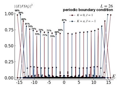
We show the overlaps between the FSA wavefunctions and the eigenstates, |E|FSAi|2superscriptinner-product𝐸subscriptFSA𝑖2|\langle E|\text{FSA}_{i}\rangle|^{2}, for i=0,1,,L𝑖01𝐿i=0,1,\dots,L in Fig. S1. We also quote the overlap values on the “matching” primary Z2subscript𝑍2Z_{2} scar states, i.e., between |FSAiketsubscriptFSA𝑖|\text{FSA}_{i}\rangle and the i𝑖i-th primary scar state, with both sets of states assumed ordered by energy. In general, the FSA provides very good approximations for the primary Z2subscript𝑍2Z_{2} scar states, and, in particular, an extremely good approximation for the ground state and the scar state closest to the ground state.

It is interesting to note that the FSA variational space and the FSA states |FSAiketsubscriptFSA𝑖|\text{FSA}_{i}\rangle generated by the above procedure do not respect the translation and inversion symmetries of the Hamiltonian. Instead, they mix the K=0𝐾0K=0, I=1𝐼1I=1 and K=π𝐾𝜋K=\pi, I=1𝐼1I=-1 sectors. However, each individual |FSAiketsubscriptFSA𝑖|\text{FSA}_{i}\rangle state generally has a very high weight on a particular symmetry sector. In principle, one can fix this completely by including the symmetry-related counterparts in the variational basis, but we have not done such an embellishment and only followed the original procedure in Refs. Turner et al. (2018a, b). On the other hand, our trial SMA and MMA wavefunctions are constructed with definite symmetry quantum numbers from the outset.
Refer to caption
Figure S1: Overlaps between the FSA wavefunctions, |FSAiketsubscriptFSA𝑖|\text{FSA}_{i}\rangle, i=0,1,,L𝑖01𝐿i=0,1,\dots,L, and the eigenstates in the PBC chain with L=26𝐿26L=26. The red lines are in the K=0𝐾0K=0, I=1𝐼1I=1 sector, while the blue lines are in the K=π𝐾𝜋K=\pi, I=1𝐼1I=-1 sector. |FSAiketsubscriptFSA𝑖|\text{FSA}_{i}\rangle has the largest overlap with the i𝑖i-th Z2subscript𝑍2Z_{2} scar state, and this value is listed for easy reference for i=0,1,,L/2𝑖01𝐿2i=0,1,\dots,L/2.

X Additional details and results of single-mode approximation and multi-mode approximation

X.1 Details of SMA for the E±1.33𝐸plus-or-minus1.33E\approx\pm 1.33 scar states with I=(1)Lb1𝐼superscript1subscript𝐿𝑏1I=(-1)^{L_{b}-1} in the main text

In the main text, we presented the “single-mode approximation” (SMA) with the translation quantum number (1)Lb1superscript1subscript𝐿𝑏1(-1)^{L_{b}-1} and inversion quantum number (1)Lb1superscript1subscript𝐿𝑏1(-1)^{L_{b}-1} to capture the scar states with energy E±1.33𝐸plus-or-minus1.33E\approx\pm 1.33. For ease of reference, we remind the construction and then explain more details behind it: |Ξ1=(|M1(1)LbTx|M1)/ξ1ketsubscriptΞ1ketsubscript𝑀1superscript1subscript𝐿𝑏subscript𝑇𝑥ketsubscript𝑀1subscript𝜉1|\Xi_{1}\rangle=(|M_{1}\rangle-(-1)^{L_{b}}T_{x}|M_{1}\rangle)/\xi_{1}, where ξ1subscript𝜉1\xi_{1} provides normalization Ξ1|Ξ1=1inner-productsubscriptΞ1subscriptΞ11\langle\Xi_{1}|\Xi_{1}\rangle=1 and

|M1=b=1LbTr[Bσ1Cσ2Mσ2b1σ2bBσL1CσL]|σ1σL,ketsubscript𝑀1superscriptsubscript𝑏1subscript𝐿𝑏Trdelimited-[]superscript𝐵subscript𝜎1superscript𝐶subscript𝜎2superscript𝑀subscript𝜎2𝑏1subscript𝜎2𝑏superscript𝐵subscript𝜎𝐿1superscript𝐶subscript𝜎𝐿ketsubscript𝜎1subscript𝜎𝐿|M_{1}\rangle=\sum_{b=1}^{L_{b}}\text{Tr}[B^{\sigma_{1}}C^{\sigma_{2}}\dots M^{\sigma_{2b-1}\sigma_{2b}}\dots B^{\sigma_{L-1}}C^{\sigma_{L}}]|\sigma_{1}\dots\sigma_{L}\rangle~{}, (S30)

with

M00=(1001),M01=(μ10μ20),M10=(00μ2μ1),M11=02×2.formulae-sequencesuperscript𝑀00matrix1001formulae-sequencesuperscript𝑀01matrixsubscript𝜇10subscript𝜇20formulae-sequencesuperscript𝑀10matrix00subscript𝜇2subscript𝜇1superscript𝑀11subscript022\displaystyle M^{00}=\begin{pmatrix}1&0\\ 0&1\end{pmatrix}~{},\quad M^{01}=\begin{pmatrix}\mu_{1}&0\\ \mu_{2}&0\end{pmatrix}~{},\quad M^{10}=\begin{pmatrix}0&0\\ -\mu_{2}&\mu_{1}\end{pmatrix}~{},\quad M^{11}=0_{2\times 2}~{}.

We have chosen the “excitation” matrices M𝑀M to satisfy M01B1=02×3superscript𝑀01superscript𝐵1subscript023M^{01}B^{1}=0_{2\times 3} and C1M10=03×2superscript𝐶1superscript𝑀10subscript032C^{1}M^{10}=0_{3\times 2} so that the wavefunction automatically satisfies the Rydberg blockade constraint. Furthermore, we have required that the matrices give the inversion quantum number opposite to the exact E=0𝐸0E=0 eigenstate |Φ1ketsubscriptΦ1|\Phi_{1}\rangle: By examining the action of I𝐼I on |M1ketsubscript𝑀1|M_{1}\rangle in the MPS language similar to Eq. (S14) and utilizing the same gauge transformation used in the discussion after Eq. (S14), we see that the desired inversion quantum number is achieved by requiring XIMIsXI1=Mssubscript𝑋𝐼superscriptsubscript𝑀𝐼𝑠superscriptsubscript𝑋𝐼1superscript𝑀𝑠X_{I}M_{I}^{s}X_{I}^{-1}=M^{s}, where MI00(M00)T,MI01(M10)T,MI10(M01)Tformulae-sequencesuperscriptsubscript𝑀𝐼00superscriptsuperscript𝑀00𝑇formulae-sequencesuperscriptsubscript𝑀𝐼01superscriptsuperscript𝑀10𝑇superscriptsubscript𝑀𝐼10superscriptsuperscript𝑀01𝑇M_{I}^{00}\equiv(M^{00})^{T},M_{I}^{01}\equiv(M^{10})^{T},M_{I}^{10}\equiv(M^{01})^{T}. Satisfying these conditions leads to the ansatz with two parameters μ1subscript𝜇1\mu_{1} and μ2subscript𝜇2\mu_{2} shown above. In principle, the SMA wavefunction has a “gauge redundancy”, i.e., property that Mσ1σ2Mσ1σ2+[W,Bσ1Cσ2]superscript𝑀subscript𝜎1subscript𝜎2superscript𝑀subscript𝜎1subscript𝜎2𝑊superscript𝐵subscript𝜎1superscript𝐶subscript𝜎2M^{\sigma_{1}\sigma_{2}}\to M^{\sigma_{1}\sigma_{2}}+[W,B^{\sigma_{1}}C^{\sigma_{2}}] does not change |M1ketsubscript𝑀1|M_{1}\rangle for arbitrary 2×2222\times 2 matrix W𝑊W. We need to consider this redundancy to find the set of truly independent parameters. In the present case, it happens that the above ansatz for the excitation matrices has independent parameters already. Hence, the gauge redundancy does not reduce the number of the independent parameters. The optimal parameters are obtained by minimizing the energy fluctuation σH2Ξ1|H2|Ξ1Ξ1|H|Ξ12subscriptsuperscript𝜎2𝐻quantum-operator-productsubscriptΞ1superscript𝐻2subscriptΞ1superscriptquantum-operator-productsubscriptΞ1𝐻subscriptΞ12\sigma^{2}_{H}\equiv\langle\Xi_{1}|H^{2}|\Xi_{1}\rangle-\langle\Xi_{1}|H|\Xi_{1}\rangle^{2}. The resulting optimal state is presented in the main text and also reproduced in Fig. S2.

We also note that by choosing μ1=μ1superscriptsubscript𝜇1subscript𝜇1\mu_{1}^{\prime}=-\mu_{1} and μ2=μ2superscriptsubscript𝜇2subscript𝜇2\mu_{2}^{\prime}=\mu_{2}, we can obtain the opposite-energy counterpart, |Ξ1𝒞ph|Ξ1similar-toketsuperscriptsubscriptΞ1subscript𝒞phketsubscriptΞ1|\Xi_{1}^{\prime}\rangle\sim\mathcal{C}_{\text{ph}}|\Xi_{1}\rangle. This can be seen using the gauge transformation introduced in the discussion of the action of 𝒞phsubscript𝒞ph\mathcal{C}_{\text{ph}} on the exact eigenstate |Φ1ketsubscriptΦ1|\Phi_{1}\rangle in Sec. IV and noting that the corresponding excitation matrices satisfy (M)s=XcMcsXc1superscriptsuperscript𝑀𝑠subscript𝑋𝑐superscriptsubscript𝑀𝑐𝑠superscriptsubscript𝑋𝑐1(M^{\prime})^{s}=X_{c}M_{c}^{s}X_{c}^{-1}, where Mc00M00,Mc01M01,Mc10M10formulae-sequencesuperscriptsubscript𝑀𝑐00superscript𝑀00formulae-sequencesuperscriptsubscript𝑀𝑐01superscript𝑀01superscriptsubscript𝑀𝑐10superscript𝑀10M_{c}^{00}\equiv M^{00},M_{c}^{01}\equiv-M^{01},M_{c}^{10}\equiv-M^{10}.

Finally, we can provide some intuition for the energetics of the SMA ansatz by working in the blocked language used in Sec. I utilizing the ±,𝟎plus-or-minus0\bm{\pm},\bm{0} basis introduced in Eq. (S8). Recall that in this basis |Φ1ketsubscriptΦ1|\Phi_{1}\rangle is conveniently written using MPS matrices in Eq. (S10). We can easily obtain excitation matrices in this representation by following the same steps that produced Eq. (S10); we find

M+=μ1+22(1001),M=μ122(1001),M𝟎=12(μ2μ1+μ2μ1μ2μ2).formulae-sequencesuperscript𝑀subscript𝜇122matrix1001formulae-sequencesuperscript𝑀subscript𝜇122matrix1001superscript𝑀012matrixsubscript𝜇2subscript𝜇1subscript𝜇2subscript𝜇1subscript𝜇2subscript𝜇2\displaystyle M^{\bm{+}}=\frac{\mu_{1}+\sqrt{2}}{2}\begin{pmatrix}1&0\\ 0&1\end{pmatrix}~{},\quad M^{\bm{-}}=\frac{\mu_{1}-\sqrt{2}}{2}\begin{pmatrix}1&0\\ 0&1\end{pmatrix}~{},\quad M^{\bm{0}}=\frac{1}{\sqrt{2}}\begin{pmatrix}\mu_{2}&\mu_{1}+\mu_{2}\\ \mu_{1}-\mu_{2}&-\mu_{2}\end{pmatrix}~{}. (S31)

We can now examine a wavefunction obtained by placing such an excitation on one block-site b𝑏b. The wavefunction has a part with sb=+subscript𝑠𝑏s_{b}=\bm{+}, originating from M+superscript𝑀M^{\bm{+}}, which on the rest of the system is basically Tr[AAA]Trdelimited-[]𝐴𝐴𝐴\text{Tr}[AA\dots A] and hence contains only configurations with equal numbers of +\bm{+} and \bm{-} block-sites. Hence, this part is an eigenstate of Hsuperscript𝐻H^{\prime} introduced in Sec. I, see Eqs. (S4) and (S9), with eigenvalue 22\sqrt{2}. Similarly, a part of the wavefunction with sb=subscript𝑠𝑏s_{b}=\bm{-}, originating from Msuperscript𝑀M^{\bm{-}}, on the rest of the system contains only configurations with equal numbers of +\bm{+} and \bm{-} block-sites; hence, this part is an eigenstate of Hsuperscript𝐻H^{\prime} with eigenvalue 22-\sqrt{2}. Note that the amplitudes of the two parts are proportional to (μ1+2)/2subscript𝜇122(\mu_{1}+\sqrt{2})/2 and (μ12)/2subscript𝜇122(\mu_{1}-\sqrt{2})/2 respectively, and for the optimal parameters μ11.09subscript𝜇11.09\mu_{1}\approx-1.09, μ20.63subscript𝜇20.63\mu_{2}\approx-0.63 used in the main text, the latter amplitude is significantly larger.

We now examine a part of the wavefunction with sb=𝟎subscript𝑠𝑏0s_{b}=\bm{0}, originating from M𝟎superscript𝑀0M^{\bm{0}}, which we further subdivide as follows. The upper-left subpart μ2/2subscript𝜇22\mu_{2}/\sqrt{2} in M𝟎superscript𝑀0M^{\bm{0}} by itself requires that on the rest of the system we have equal numbers of +\bm{+}’s and \bm{-}’s, and the first such site to the right of b𝑏b must be +\bm{+}. Similarly, the lower-right subpart μ2/2subscript𝜇22-\mu_{2}/\sqrt{2} in M𝟎superscript𝑀0M^{\bm{0}} by itself requires that on the rest of the system we have equal numbers of +\bm{+}’s and \bm{-}’s, and the first such site to the right of b𝑏b must be \bm{-}. Each of these cases gives an eigenstate of Hsuperscript𝐻H^{\prime} with eigenvalue 00. Next, the lower-left subpart (μ1μ2)/2subscript𝜇1subscript𝜇22(\mu_{1}-\mu_{2})/\sqrt{2} in M𝟎superscript𝑀0M^{\bm{0}} by itself requires configurations on the rest of the system to be of the form ++\dots\bm{+}\dots\bm{-}\dots\bm{+}\dots, where “\dots” can contain any number of 𝟎0\bm{0}’s. Such configurations contain one more +\bm{+} compared to \bm{-}, which gives an eigenstate of Hsuperscript𝐻H^{\prime} with eigenvalue 22\sqrt{2}. Similarly, the upper-right subpart (μ1+μ2)/2subscript𝜇1subscript𝜇22(\mu_{1}+\mu_{2})/\sqrt{2} in M𝟎superscript𝑀0M^{\bm{0}} by itself requires configurations on the rest of the system to be of the form +\dots\bm{-}\dots\bm{+}\dots\bm{-}\dots, i.e., contain one less +\bm{+} compared to \bm{-}, which gives an eigenstate of Hsuperscript𝐻H^{\prime} with eigenvalue 22-\sqrt{2}.

We can now use the fact that the expectation value of H𝐻H in this wavefunction coincides with the expectation value of Hsuperscript𝐻H^{\prime}, since the genuinely two-body parts in the writing of H𝐻H in Sec. I connect to outside of the Rydberg-constrained Hilbert space. (As a side remark, we can obtain the action of H𝐻H on this wavefunction by first acting with Hsuperscript𝐻H^{\prime} and then projecting into the Rydberg Hilbert space; in particular, one can see that such an excitation wavefunction is no longer exact eigenstate of H𝐻H.) By examining contributions to the expectation value of Hsuperscript𝐻H^{\prime} from the above parts of the wavefunction, we can roughly understand the value of the trial energy 1.31absent1.31\approx-1.31 obtained using these excitation matrices in the main text. Also, we can see that changing the sign of μ1subscript𝜇1\mu_{1} gives a trial state with opposite energy, in agreement with the formal argument using 𝒞phsubscript𝒞ph\mathcal{C}_{\text{ph}} given earlier.

Note that in the main text we formed plane wave superpositions of such localized excitations, and in the analysis here we are not attempting a quantitative match with the numerical results. Also note that while this analysis provides a rough intuition for the trial energies, in the main text we optimized the SMA ansatz by minimizing the variance, for which we have less intuition. Nevertheless, the above arguments provide an approximate picture where adding an excitation is like acting with a ladder operator raising or lowering eigenvalues of Hsuperscript𝐻H^{\prime} in Eq. (S9), and developing this picture more precisely may provide a better understanding of the scar states in the PXP model away from E=0𝐸0E=0.

X.2 SMA for the E±2.66𝐸plus-or-minus2.66E\approx\pm 2.66 scar states with I=(1)Lb𝐼superscript1subscript𝐿𝑏I=(-1)^{L_{b}}

While in the main text we showed the multi-mode approximation (MMA) to capture other Z2subscript𝑍2Z_{2} scar states, here we can also try to use the SMA but with the symmetry quantum numbers Tx=(1)Lbsubscript𝑇𝑥superscript1subscript𝐿𝑏T_{x}=(-1)^{L_{b}} and I=(1)Lb𝐼superscript1subscript𝐿𝑏I=(-1)^{L_{b}}. Specifically, we can write an SMA wavefunction with such quantum numbers as |Ξ~1=(|M~1+(1)LbTx|M~1)/ξ~1ketsubscript~Ξ1ketsubscript~𝑀1superscript1subscript𝐿𝑏subscript𝑇𝑥ketsubscript~𝑀1subscript~𝜉1|\tilde{\Xi}_{1}\rangle=(|\tilde{M}_{1}\rangle+(-1)^{L_{b}}T_{x}|\tilde{M}_{1}\rangle)/\tilde{\xi}_{1}, where again ξ~1subscript~𝜉1\tilde{\xi}_{1} is the normalization factor and |M~1ketsubscript~𝑀1|\tilde{M}_{1}\rangle has the same form as in Eq. (S30) but with matrices

M~00=(22μ~12μ~12),M~01=(μ~1010),M~10=(001μ~1).formulae-sequencesuperscript~𝑀00matrix22subscript~𝜇12subscript~𝜇12formulae-sequencesuperscript~𝑀01matrixsubscript~𝜇1010superscript~𝑀10matrix001subscript~𝜇1\displaystyle\tilde{M}^{00}=\begin{pmatrix}\sqrt{2}&-\sqrt{2}\tilde{\mu}_{1}\\ \sqrt{2}\tilde{\mu}_{1}&-\sqrt{2}\end{pmatrix}~{},\quad\tilde{M}^{01}=\begin{pmatrix}-\tilde{\mu}_{1}&0\\ -1&0\end{pmatrix}~{},\quad\tilde{M}^{10}=\begin{pmatrix}0&0\\ -1&\tilde{\mu}_{1}\end{pmatrix}~{}.

Similarly to the construction of |M1ketsubscript𝑀1|M_{1}\rangle, we have chosen the matrices M~ssuperscript~𝑀𝑠\tilde{M}^{s} to satisfy M~01B1=02×3superscript~𝑀01superscript𝐵1subscript023\tilde{M}^{01}B^{1}=0_{2\times 3} and C1M~10=03×2superscript𝐶1superscript~𝑀10subscript032C^{1}\tilde{M}^{10}=0_{3\times 2} but with XIM~IsXI1=M~ssubscript𝑋𝐼superscriptsubscript~𝑀𝐼𝑠superscriptsubscript𝑋𝐼1superscript~𝑀𝑠X_{I}\tilde{M}_{I}^{s}X_{I}^{-1}=-\tilde{M}^{s} to give the same inversion quantum number as |ΦiketsubscriptΦ𝑖|\Phi_{i}\rangle. We have also used the SMA gauge redundancy, M~σ1σ2M~σ1σ2+[W,Bσ1Cσ2]superscript~𝑀subscript𝜎1subscript𝜎2superscript~𝑀subscript𝜎1subscript𝜎2𝑊superscript𝐵subscript𝜎1superscript𝐶subscript𝜎2\tilde{M}^{\sigma_{1}\sigma_{2}}\to\tilde{M}^{\sigma_{1}\sigma_{2}}+[W,B^{\sigma_{1}}C^{\sigma_{2}}], to identify the truly independent parameters. Finally, the number of the independent parameters was reduced by one by requiring |M~1ketsubscript~𝑀1|\tilde{M}_{1}\rangle to be orthogonal to |Φ1ketsubscriptΦ1|\Phi_{1}\rangle in the thermodynamic limit (we did not need to do this for |M1ketsubscript𝑀1|M_{1}\rangle since it has different inversion quantum number and is automatically orthogonal to |Φ1ketsubscriptΦ1|\Phi_{1}\rangle).

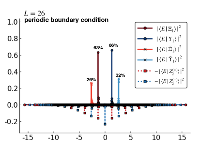
The optimal parameter μ~1subscript~𝜇1\tilde{\mu}_{1} is obtained by minimizing the energy fluctuation; using system of length L=26𝐿26L=26, we find μ~1=0.89285subscript~𝜇10.89285\tilde{\mu}_{1}=0.89285, Ξ~1|H|Ξ~1=2.4572quantum-operator-productsubscript~Ξ1𝐻subscript~Ξ12.4572\langle\tilde{\Xi}_{1}|H|\tilde{\Xi}_{1}\rangle=-2.4572 and Ξ~1|H2|Ξ~1Ξ~1|H|Ξ~12=0.3219quantum-operator-productsubscript~Ξ1superscript𝐻2subscript~Ξ1superscriptquantum-operator-productsubscript~Ξ1𝐻subscript~Ξ120.3219\langle\tilde{\Xi}_{1}|H^{2}|\tilde{\Xi}_{1}\rangle-\langle\tilde{\Xi}_{1}|H|\tilde{\Xi}_{1}\rangle^{2}=0.3219. To obtain the positive energy counterpart, we can choose μ~1=μ~1superscriptsubscript~𝜇1subscript~𝜇1\tilde{\mu}_{1}^{\prime}=-\tilde{\mu}_{1}, which gives |Ξ~1𝒞ph|Ξ~1similar-toketsuperscriptsubscript~Ξ1subscript𝒞phketsubscript~Ξ1|\tilde{\Xi}_{1}^{\prime}\rangle\sim\mathcal{C}_{\text{ph}}|\tilde{\Xi}_{1}\rangle (the argument is essentially identical to that for |Ξ1𝒞ph|Ξ1similar-toketsuperscriptsubscriptΞ1subscript𝒞phketsubscriptΞ1|\Xi_{1}^{\prime}\rangle\sim\mathcal{C}_{\text{ph}}|\Xi_{1}\rangle at the end of the previous subsection). The overlap of |Ξ~1ketsubscript~Ξ1|\tilde{\Xi}_{1}\rangle with the eigenstates is plotted in Fig. S2. While this state still has majority of the weight on the primary scar state with E2.66𝐸2.66E\approx-2.66, the overlap is significantly worse than the multi-particle ansatz |Ξ2ketsubscriptΞ2|\Xi_{2}\rangle presented in the main text. The wavefunction |Ξ~1ketsubscript~Ξ1|\tilde{\Xi}_{1}\rangle can be loosely viewed as a bound state of two quasiparticles, while |Ξ2ketsubscriptΞ2|\Xi_{2}\rangle can be viewed as a scattering state of two quasiparticles. These results suggest that the scar states are better understood as essentially free quasiparticle states rather than bound states of quasiparticles.

X.3 “Bond-dimension-3” SMA

The SMA wavefunctions |Ξ1ketsubscriptΞ1|\Xi_{1}\rangle and |Ξ~1ketsubscript~Ξ1|\tilde{\Xi}_{1}\rangle are constructed by “exciting” the matrices B𝐵B and C𝐶C consecutively, where the “quasiparicle excitation” matrix M𝑀M has bond-dimension 2. We therefore call these wavefunctions “bond-dimension-2” ansatzes. On the other hand, one can also think of excitations on consecutive matrices C𝐶C and B𝐵B, which will give the quasiparticle excitation matrix with bond-dimension 3. Such ansatzes will have more variational parameters and can potentially be better approximations. The bond-dimension-3 SMA capturing the E±1.33𝐸plus-or-minus1.33E\approx\pm 1.33 scar states with quantum numbers Tx=(1)Lb1subscript𝑇𝑥superscript1subscript𝐿𝑏1T_{x}=(-1)^{L_{b}-1} and I=(1)Lb1𝐼superscript1subscript𝐿𝑏1I=(-1)^{L_{b}-1} is |Υ1=(|N1(1)LbTx|N1)/υ1ketsubscriptΥ1ketsubscript𝑁1superscript1subscript𝐿𝑏subscript𝑇𝑥ketsubscript𝑁1subscript𝜐1|\Upsilon_{1}\rangle=(|N_{1}\rangle-(-1)^{L_{b}}T_{x}|N_{1}\rangle)/\upsilon_{1}, where υ1subscript𝜐1\upsilon_{1} is the normalization factor and

|N1=b=1LbTr[Bσ1Cσ2Bσ2b1Nσ2bσ2b+1Cσ2b+2BσL1CσL]|σ1σL,ketsubscript𝑁1superscriptsubscript𝑏1subscript𝐿𝑏Trdelimited-[]superscript𝐵subscript𝜎1superscript𝐶subscript𝜎2superscript𝐵subscript𝜎2𝑏1superscript𝑁subscript𝜎2𝑏subscript𝜎2𝑏1superscript𝐶subscript𝜎2𝑏2superscript𝐵subscript𝜎𝐿1superscript𝐶subscript𝜎𝐿ketsubscript𝜎1subscript𝜎𝐿|N_{1}\rangle=\sum_{b=1}^{L_{b}}\text{Tr}[B^{\sigma_{1}}C^{\sigma_{2}}\dots B^{\sigma_{2b-1}}N^{\sigma_{2b}\sigma_{2b+1}}C^{\sigma_{2b+2}}\dots B^{\sigma_{L-1}}C^{\sigma_{L}}]|\sigma_{1}\dots\sigma_{L}\rangle~{}, (S32)

with

N00=(1+2ν7022ν6012ν722ν522ν622ν5ν1),N01=(ν22ν6ν2ν6+ν7ν3ν6+ν7ν2ν5ν4ν2ν5),N10=(ν2ν6+ν7ν2ν52ν6ν3ν4ν2ν6ν7ν2+ν5).formulae-sequencesuperscript𝑁00matrix12subscript𝜈7022subscript𝜈6012subscript𝜈722subscript𝜈522subscript𝜈622subscript𝜈5subscript𝜈1formulae-sequencesuperscript𝑁01matrixsubscript𝜈22subscript𝜈6subscript𝜈2subscript𝜈6subscript𝜈7subscript𝜈3subscript𝜈6subscript𝜈7subscript𝜈2subscript𝜈5subscript𝜈4subscript𝜈2subscript𝜈5superscript𝑁10matrixsubscript𝜈2subscript𝜈6subscript𝜈7subscript𝜈2subscript𝜈52subscript𝜈6subscript𝜈3subscript𝜈4subscript𝜈2subscript𝜈6subscript𝜈7subscript𝜈2subscript𝜈5\displaystyle N^{00}=\begin{pmatrix}1+\sqrt{2}\,\nu_{7}&0&2\sqrt{2}\,\nu_{6}\\ 0&1-\sqrt{2}\,\nu_{7}&2\sqrt{2}\,\nu_{5}\\ -2\sqrt{2}\,\nu_{6}&2\sqrt{2}\,\nu_{5}&\nu_{1}\end{pmatrix}~{},~{}~{}N^{01}=\begin{pmatrix}\nu_{2}&2\nu_{6}&\nu_{2}\\ \nu_{6}+\nu_{7}&\nu_{3}&\nu_{6}+\nu_{7}\\ \nu_{2}-\nu_{5}&\nu_{4}&\nu_{2}-\nu_{5}\end{pmatrix}~{},~{}~{}N^{10}=\begin{pmatrix}\nu_{2}&\nu_{6}+\nu_{7}&-\nu_{2}-\nu_{5}\\ 2\nu_{6}&\nu_{3}&-\nu_{4}\\ -\nu_{2}&-\nu_{6}-\nu_{7}&\nu_{2}+\nu_{5}\end{pmatrix}~{}.

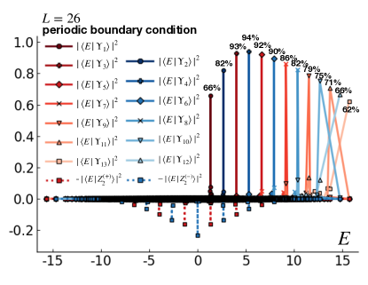
We obtained these matrices by requiring N01C1=03×2superscript𝑁01superscript𝐶1subscript032N^{01}C^{1}=0_{3\times 2}, B1N10=02×3superscript𝐵1superscript𝑁10subscript023B^{1}N^{10}=0_{2\times 3} to ensure the Rydberg constraints. To obtain the desired inversion quantum number, we also required YINIsYI1=Nssubscript𝑌𝐼superscriptsubscript𝑁𝐼𝑠superscriptsubscript𝑌𝐼1superscript𝑁𝑠Y_{I}N_{I}^{s}Y_{I}^{-1}=N^{s}, where NI00(N00)Tsuperscriptsubscript𝑁𝐼00superscriptsuperscript𝑁00𝑇N_{I}^{00}\equiv(N^{00})^{T}, NI01(N10)Tsuperscriptsubscript𝑁𝐼01superscriptsuperscript𝑁10𝑇N_{I}^{01}\equiv(N^{10})^{T}, NI10(N01)Tsuperscriptsubscript𝑁𝐼10superscriptsuperscript𝑁01𝑇N_{I}^{10}\equiv(N^{01})^{T}, and YIsubscript𝑌𝐼Y_{I} is the matrix for the gauge transformation used in our discussion of I𝐼I in Sec. IV. Finally, we also used the SMA gauge redundancy, Nσ1σ2Nσ1σ2+[W,Cσ1Bσ2]superscript𝑁subscript𝜎1subscript𝜎2superscript𝑁subscript𝜎1subscript𝜎2𝑊superscript𝐶subscript𝜎1superscript𝐵subscript𝜎2N^{\sigma_{1}\sigma_{2}}\to N^{\sigma_{1}\sigma_{2}}+[W,C^{\sigma_{1}}B^{\sigma_{2}}], to find truly independent parameters as shown above. For system size L=26𝐿26L=26, we find the optimal parameters ν1=0.507183subscript𝜈10.507183\nu_{1}=0.507183, ν2=0.60202subscript𝜈20.60202\nu_{2}=0.60202, ν3=0.625366subscript𝜈30.625366\nu_{3}=0.625366, ν4=0.264115subscript𝜈40.264115\nu_{4}=0.264115, ν5=0.00128607subscript𝜈50.00128607\nu_{5}=-0.00128607, ν6=0.0228075subscript𝜈60.0228075\nu_{6}=0.0228075, and ν7=0.42342subscript𝜈70.42342\nu_{7}=0.42342. The trial energy is Υ1|H|Υ1=1.3396quantum-operator-productsubscriptΥ1𝐻subscriptΥ11.3396\langle\Upsilon_{1}|H|\Upsilon_{1}\rangle=1.3396 and the energy fluctuation is Υ1|H2|Υ1Υ1|H|Υ12=0.007201quantum-operator-productsubscriptΥ1superscript𝐻2subscriptΥ1superscriptquantum-operator-productsubscriptΥ1𝐻subscriptΥ120.007201\langle\Upsilon_{1}|H^{2}|\Upsilon_{1}\rangle-\langle\Upsilon_{1}|H|\Upsilon_{1}\rangle^{2}=0.007201, which is a more accurate approximation than the |Ξ1ketsubscriptΞ1|\Xi_{1}\rangle SMA state in the main text. We can see from Fig. S2 that the overlap with the primary Z2subscript𝑍2Z_{2} scar state with energy E1.33𝐸1.33E\approx 1.33 is 66%percent6666\%, which is higher than the bond-dimension-2 ansatz |Ξ1ketsubscriptΞ1|\Xi_{1}\rangle. To obtain the negative energy counterpart, one can simply change the signs of ν2,3,5subscript𝜈235\nu_{2,3,5} and obtain |Υ1𝒞ph|Υ1similar-toketsuperscriptsubscriptΥ1subscript𝒞phketsubscriptΥ1|\Upsilon_{1}^{\prime}\rangle\sim\mathcal{C}_{\text{ph}}|\Upsilon_{1}\rangle, which is deduced by applying the discussion of 𝒞phsubscript𝒞ph\mathcal{C}_{\text{ph}} in Sec. IV and using (N)s=YcNcsYc1superscriptsuperscript𝑁𝑠subscript𝑌𝑐superscriptsubscript𝑁𝑐𝑠superscriptsubscript𝑌𝑐1(N^{\prime})^{s}=Y_{c}N_{c}^{s}Y_{c}^{-1}, where Nc00N00,Nc01N01,Nc10N10formulae-sequencesuperscriptsubscript𝑁𝑐00superscript𝑁00formulae-sequencesuperscriptsubscript𝑁𝑐01superscript𝑁01superscriptsubscript𝑁𝑐10superscript𝑁10N_{c}^{00}\equiv N^{00},N_{c}^{01}\equiv-N^{01},N_{c}^{10}\equiv-N^{10}.

Similarly, we can construct the bond-dimension-3 SMA in the symmetry sector Tx=(1)Lbsubscript𝑇𝑥superscript1subscript𝐿𝑏T_{x}=(-1)^{L_{b}} and I=(1)Lb𝐼superscript1subscript𝐿𝑏I=(-1)^{L_{b}} as |Υ~1=(|N~1+(1)LbTx|N~1)/υ~1ketsubscript~Υ1ketsubscript~𝑁1superscript1subscript𝐿𝑏subscript𝑇𝑥ketsubscript~𝑁1subscript~𝜐1|\tilde{\Upsilon}_{1}\rangle=(|\tilde{N}_{1}\rangle+(-1)^{L_{b}}T_{x}|\tilde{N}_{1}\rangle)/\tilde{\upsilon}_{1}, where υ~1subscript~𝜐1\tilde{\upsilon}_{1} is the normalization factor and |N~1ketsubscript~𝑁1|\tilde{N}_{1}\rangle has the same form as in Eq. (S32) but with matrices

N~00=(02222ν~422022ν~322ν~422ν~30),N~01=(12ν~41ν~4ν~1ν~41+ν~3ν~21+ν~3),N~10=(1ν~41ν~32ν~4ν~1ν~21ν~41+ν~3).formulae-sequencesuperscript~𝑁00matrix02222subscript~𝜈422022subscript~𝜈322subscript~𝜈422subscript~𝜈30formulae-sequencesuperscript~𝑁01matrix12subscript~𝜈41subscript~𝜈4subscript~𝜈1subscript~𝜈41subscript~𝜈3subscript~𝜈21subscript~𝜈3superscript~𝑁10matrix1subscript~𝜈41subscript~𝜈32subscript~𝜈4subscript~𝜈1subscript~𝜈21subscript~𝜈41subscript~𝜈3\displaystyle\tilde{N}^{00}=\begin{pmatrix}0&2\sqrt{2}&2\sqrt{2}\,\tilde{\nu}_{4}\\ -2\sqrt{2}&0&2\sqrt{2}\,\tilde{\nu}_{3}\\ 2\sqrt{2}\;\tilde{\nu}_{4}&-2\sqrt{2}\,\tilde{\nu}_{3}&0\end{pmatrix}~{},~{}~{}\tilde{N}^{01}=\begin{pmatrix}-1&-2\tilde{\nu}_{4}&-1\\ \tilde{\nu}_{4}&\tilde{\nu}_{1}&\tilde{\nu}_{4}\\ -1+\tilde{\nu}_{3}&\tilde{\nu}_{2}&-1+\tilde{\nu}_{3}\end{pmatrix}~{},~{}~{}\tilde{N}^{10}=\begin{pmatrix}1&-\tilde{\nu}_{4}&-1-\tilde{\nu}_{3}\\ 2\tilde{\nu}_{4}&-\tilde{\nu}_{1}&\tilde{\nu}_{2}\\ -1&\tilde{\nu}_{4}&1+\tilde{\nu}_{3}\end{pmatrix}~{}.

In addition to satisfying the Rydberg constraint and giving the inversion quantum number I=(1)Lb𝐼superscript1subscript𝐿𝑏I=(-1)^{L_{b}}, the matrices are chosen such that |Υ~1ketsubscript~Υ1|\tilde{\Upsilon}_{1}\rangle is orthogonal to |Φ1ketsubscriptΦ1|\Phi_{1}\rangle in the thermodynamic limit. Using system size L=26𝐿26L=26, we find the optimal parameters ν~1=2.59334subscript~𝜈12.59334\tilde{\nu}_{1}=2.59334, ν~2=1.48065subscript~𝜈21.48065\tilde{\nu}_{2}=1.48065, ν~3=0.0615383subscript~𝜈30.0615383\tilde{\nu}_{3}=0.0615383, and ν~4=0.992914subscript~𝜈40.992914\tilde{\nu}_{4}=-0.992914, with the trial energy Υ~1|H|Υ~1=2.5594quantum-operator-productsubscript~Υ1𝐻subscript~Υ12.5594\langle\tilde{\Upsilon}_{1}|H|\tilde{\Upsilon}_{1}\rangle=2.5594, and energy fluctuation Υ~1|H2|Υ~1Υ~1|H|Υ~12=0.18591quantum-operator-productsubscript~Υ1superscript𝐻2subscript~Υ1superscriptquantum-operator-productsubscript~Υ1𝐻subscript~Υ120.18591\langle\tilde{\Upsilon}_{1}|H^{2}|\tilde{\Upsilon}_{1}\rangle-\langle\tilde{\Upsilon}_{1}|H|\tilde{\Upsilon}_{1}\rangle^{2}=0.18591. To obtain the corresponding negative-energy trial state |Υ~1𝒞ph|Υ~1similar-toketsubscriptsuperscript~Υ1subscript𝒞phketsubscript~Υ1|\tilde{\Upsilon}^{\prime}_{1}\rangle\sim\mathcal{C}_{\text{ph}}|\tilde{\Upsilon}_{1}\rangle, one changes the signs of ν~2subscript~𝜈2\tilde{\nu}_{2} and ν~4subscript~𝜈4\tilde{\nu}_{4}. We again see from Fig. S2 that the overlap with the Z2subscript𝑍2Z_{2} primary scar state at E2.66𝐸2.66E\approx 2.66 is higher than the bond-dimension-2 ansatz |Ξ~1ketsubscript~Ξ1|\tilde{\Xi}_{1}\rangle, but significantly worse than the MMA wavefunction |Ξ2ketsubscriptΞ2|\Xi_{2}\rangle.

Refer to caption
Figure S2: Overlaps of the SMA wavefunctions with eigenstates in the PBC chain of length L=26𝐿26L=26. Here the SMA wavefunctions are constructed using “bond-dimension 2” (|Ξ1ketsubscriptΞ1|\Xi_{1}\rangle and |Ξ~1ketsubscript~Ξ1|\tilde{\Xi}_{1}\rangle) and “bond-dimension 3” (|Υ1ketsubscriptΥ1|\Upsilon_{1}\rangle and |Υ~1ketsubscript~Υ1|\tilde{\Upsilon}_{1}\rangle) ansatzes, with choices producing different symmetry sectors. The red lines and the non-tilde states label the K=0𝐾0K=0, I=1𝐼1I=1 sector; while the blue lines and the tilded states label the K=π𝐾𝜋K=\pi, I=1𝐼1I=-1 sector.

In fact, we can again construct the corresponding “bond-dimension-3” MMA wavefunctions: |Υn=(|Nn+(1)Lb+nTx|Nn)/υnketsubscriptΥ𝑛ketsubscript𝑁𝑛superscript1subscript𝐿𝑏𝑛subscript𝑇𝑥ketsubscript𝑁𝑛subscript𝜐𝑛|\Upsilon_{n}\rangle=(|N_{n}\rangle+(-1)^{L_{b}+n}T_{x}|N_{n}\rangle)/\upsilon_{n}, where

|Nn=ketsubscript𝑁𝑛absent\displaystyle|N_{n}\rangle= b1,,bn=1LbTr[Bσ1Cσ2Nσ2b1σ2b1+1Nσ2bnσ2bn+1BσL1CσL]|σ1σL,superscriptsubscriptsuperscriptsubscript𝑏1subscript𝑏𝑛1subscript𝐿𝑏Trdelimited-[]superscript𝐵subscript𝜎1superscript𝐶subscript𝜎2superscript𝑁subscript𝜎2subscript𝑏1subscript𝜎2subscript𝑏11superscript𝑁subscript𝜎2subscript𝑏𝑛subscript𝜎2subscript𝑏𝑛1superscript𝐵subscript𝜎𝐿1superscript𝐶subscript𝜎𝐿ketsubscript𝜎1subscript𝜎𝐿\displaystyle\sideset{}{{}^{\prime}}{\sum}_{b_{1},\dots,b_{n}=1}^{L_{b}}\text{Tr}[B^{\sigma_{1}}C^{\sigma_{2}}\dots N^{\sigma_{2b_{1}}\sigma_{2b_{1}+1}}\dots N^{\sigma_{2b_{n}}\sigma_{2b_{n}+1}}\dots B^{\sigma_{L-1}}C^{\sigma_{L}}]|\sigma_{1}\dots\sigma_{L}\rangle~{}, (S33)

the summation is constrained to have all bisubscript𝑏𝑖b_{i} distinct, and υnsubscript𝜐𝑛\upsilon_{n} is the normalization factor. We take the N𝑁N matrices from the optimal result of |Υ1ketsubscriptΥ1|\Upsilon_{1}\rangle and examine the overlaps of |ΥnketsubscriptΥ𝑛|\Upsilon_{n}\rangle with the eigenstates, in particular, with the Z2subscript𝑍2Z_{2} primary scar states in Fig. S3. Similar to the bond-dimension-2 results presented in the main text, these bond-dimension-3 MMA wavefunctions have symmetry quantum numbers Tx=I=(1)Lb+nsubscript𝑇𝑥𝐼superscript1subscript𝐿𝑏𝑛T_{x}=I=(-1)^{L_{b}+n} and, remarkably, capture the primary scar states with even higher fidelity with more quasiparticles, up to nLb/4𝑛subscript𝐿𝑏4n\approx L_{b}/4. In this case, even the ground state and the primary scar states near the ground state are approximated fairly well compared to the results from the bond-dimension-2 ansatzes |ΞnketsubscriptΞ𝑛|\Xi_{n}\rangle.

Refer to caption
Figure S3: Overlaps between the MMA wavefunctions |ΥnketsubscriptΥ𝑛|\Upsilon_{n}\rangle with eigenstates in the PBC chain with L=26𝐿26L=26. The quasiparticle N𝑁N matrices are chosen from the optimal “bond-dimension 3” SMA wavefunction. These wavefunctions represent the simplest scattering states of the quasiparticles with hard-core exclusions.

XI Size dependence of the bipartite entanglement entropy of SMA and MMA
Refer to caption
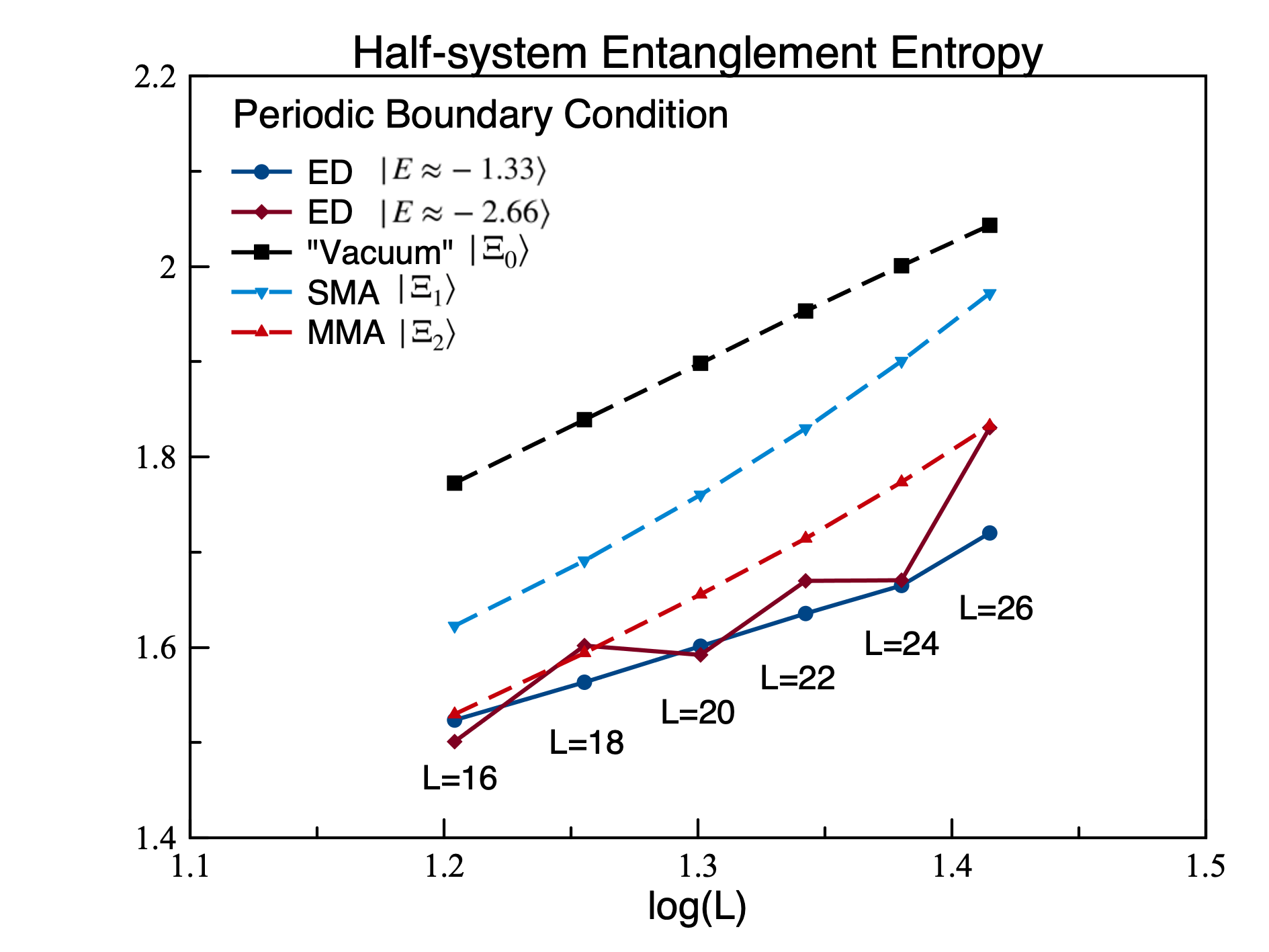
Figure S4: Bipartite entanglement entropies of the exact eigenstates and the variational SMA and MMA states. The primary scar states with E1.33𝐸1.33E\approx-1.33 and E2.66𝐸2.66E\approx-2.66 show what appears to be logarithmic scaling for the available system sizes L𝐿L. The “vacuum” |Ξ0[|Φ1+(1)Lb|Φ2]/ξ0ketsubscriptΞ0delimited-[]ketsubscriptΦ1superscript1subscript𝐿𝑏ketsubscriptΦ2subscript𝜉0|\Xi_{0}\rangle\equiv[|\Phi_{1}\rangle+(-1)^{L_{b}}|\Phi_{2}\rangle]/\xi_{0} (i.e., exact E=0𝐸0E=0 wavefunction with appropriate momentum) and the SMA/MMA |Ξ1ketsubscriptΞ1|\Xi_{1}\rangle and |Ξ2ketsubscriptΞ2|\Xi_{2}\rangle are expected to have constant entanglement scaling at large L𝐿L, while they also show apparent logarithmic scaling at these small system sizes. Note that for the optimal SMA and MMA we found, adding quasiparticles in fact decreases the entnaglement entropies.

In this section, we discuss the bipartite entanglement entropy scaling of the SMA and MMA wavefunctions comparing with the ED results. In Fig. S4, we show the bipartite entanglement entropy at small system sizes reachable by ED, obtained for chains in PBC for dividing the system into halves. For the primary scar states at E1.33𝐸1.33E\approx-1.33 and E2.66𝐸2.66E\approx-2.66, their entanglement entropies show seeming logarithmic scaling, and are conjectured in Ref. Turner et al. (2018b) to have such scaling in the thermodynamic limit. On the other hand, the “vacuum” wavefunction of the quasiparticles, |Ξ0[|Φ1+(1)Lb|Φ2]/ξ0ketsubscriptΞ0delimited-[]ketsubscriptΦ1superscript1subscript𝐿𝑏ketsubscriptΦ2subscript𝜉0|\Xi_{0}\rangle\equiv[|\Phi_{1}\rangle+(-1)^{L_{b}}|\Phi_{2}\rangle]/\xi_{0} (i.e., properly normalized exact E=0𝐸0E=0 eigenstate with appropriate 00 or π𝜋\pi momentum depending on Lb=L/2subscript𝐿𝑏𝐿2L_{b}=L/2), has constant entanglement scaling in the thermodynamic limit with the saturation value S2.254𝑆2.254S\approx 2.254, see the main text for details. Since they add only a finite number of quasiparticles, the SMA and MMA wavefunctions |Ξ1ketsubscriptΞ1|\Xi_{1}\rangle and |Ξ2ketsubscriptΞ2|\Xi_{2}\rangle are also expected to have constant entanglement scaling in the thermodynamic limit. However, as we can see from Fig. S4, the vacuum |Ξ0ketsubscriptΞ0|\Xi_{0}\rangle and the SMA and MMA |Ξ1,2ketsubscriptΞ12|\Xi_{1,2}\rangle wavefunctions also show apparent logarithmic entanglement scaling and bound the entanglement of the primary scar states at the available small system sizes. It is also noteworthy that in our SMA and MMA wavefunctions, adding quasiparticles in fact decreases the entanglement entropy; this is contrary to common intuition about adding quasiparticles on top of a ground state, but it can happen in formal MPS states and depends on the properties of the “excitation” matrices.

If the SMA and MMA wavefunctions are qualitatively true asymptotic descriptions for the primary scar states, then the seeming logarithmic entanglement scaling of the ED results could be simply finite-size effect, and to see such constant scaling behavior, one may need to go to much larger system sizes. However, while the statements about our exact E=0𝐸0E=0 scar states are exact, the SMA and MMA wavefunctions are only approximations to the ED scars. One needs to study if it is possible to construct convergent improvements of the SMA and MMA states and their true properties in the thermodynamic limit, which is a non-trivial question given the surrounding eigenstates forming apparently thermal background. We hope that addressing this question will help understanding stability of the scar states in the thermodynamic limit and in the presence of generic perturbations, while the presented entanglement data is meant to show that the available system sizes are still not sufficient to distinguish between constant or logarithmic entanglement scaling in the primary scar states.

XII Diagonalizing the Hamiltonian in the variational space spanned by |ΞnketsubscriptΞ𝑛|\Xi_{n}\rangle

While increasing the number of variational parameters is one way to improve the ansatzes, we can also improve the trial states starting with |ΞnketsubscriptΞ𝑛|\Xi_{n}\rangle in the same spirit as the FSA improves on the states constructed using (H+)n|Z2superscriptsuperscript𝐻𝑛ketsubscript𝑍2(H^{+})^{n}|Z_{2}\rangle. That is, we can treat the span of |ΞnketsubscriptΞ𝑛|\Xi_{n}\rangle, n=1,,Lb𝑛1subscript𝐿𝑏n=1,\dots,L_{b} as the “variational subspace” and project the Hamiltonian into this variational space (recall that Lb=L/2subscript𝐿𝑏𝐿2L_{b}=L/2, and here n𝑛n runs over the negative-energy MMA states). More specifically, we obtain an Lb×Lbsubscript𝐿𝑏subscript𝐿𝑏L_{b}\times L_{b} effective Hamiltonian Heffsubscript𝐻effH_{\text{eff}} with matrix elements [Heff]nm=Ξn|H|Ξmsubscriptdelimited-[]subscript𝐻eff𝑛𝑚quantum-operator-productsubscriptΞ𝑛𝐻subscriptΞ𝑚[H_{\text{eff}}]_{nm}=\langle\Xi_{n}|H|\Xi_{m}\rangle and the overlap matrix B𝐵B with matrix elements [B]nm=Ξn|Ξmsubscriptdelimited-[]𝐵𝑛𝑚inner-productsubscriptΞ𝑛subscriptΞ𝑚[B]_{nm}=\langle\Xi_{n}|\Xi_{m}\rangle. (Note that these matrices in fact are in block-diagonal form due to the symmetries.) We then solve the generalized eigenvalue problem Heffv(i)=λiBv(i)subscript𝐻effsuperscript𝑣𝑖subscript𝜆𝑖𝐵superscript𝑣𝑖H_{\text{eff}}\vec{v}^{(i)}=\lambda_{i}B\vec{v}^{(i)}, obtaining the improved wavefunctions n=1Lbvn(i)|Ξnsuperscriptsubscript𝑛1subscript𝐿𝑏superscriptsubscript𝑣𝑛𝑖ketsubscriptΞ𝑛\sum_{n=1}^{L_{b}}\vec{v}_{n}^{(i)}|\Xi_{n}\rangle, for i=1,,Lb𝑖1subscript𝐿𝑏i=1,\dots,L_{b}.

Figure S5 shows the overlap between the improved trial states and the eigenstates at L=26𝐿26L=26. We see that the improvements are mainly on the approximations on the scar states close to the ground state and the ground state; while the approximations to the scar states close to the middle of the spectrum are not affected much. This is expected, since, as one can see from a careful inspection of Fig. 2 in the main text, |ΞnketsubscriptΞ𝑛|\Xi_{n}\rangle’s with nLb/2greater-than-or-equivalent-to𝑛subscript𝐿𝑏2n\gtrsim L_{b}/2 have high weights on usually two primary scar states. The diagonalization procedure within this variational subspace therefore can be better isolated and improve approximations to the corresponding scar states.

To conclude, we see that, qualitatively, the primary scar states can be well understood as free quasiparticles, at least for our finite system sizes. An immediate question is if such a description survives for much larger sizes or even in the thermodynamic limit. We already see that some systematic improvements of the approximations can be achieved by increasing the number of variational parameters, as in the bond-dimension-3 SMA or allowing superpositions of the MMA states as in the present section. Some immediate improvements could be achieved also by allowing the variational parameters to vary in each individual MMA state rather than simply using the values from the optimal SMA state, and by allowing superpositions of different families of the already constructed states, such as the SMA |Ξ~1ketsubscript~Ξ1|\tilde{\Xi}_{1}\rangle and the MMA |Ξ2ketsubscriptΞ2|\Xi_{2}\rangle for the E2.66𝐸2.66E\approx-2.66 scar states, etc. A more systematic approach is to increase the excitation block size and study convergence to the exact scar states. In particular, we hope that this can tell whether the scar states truly survive in the thermodynamic limit even when they do not have exact closed-form expressions as happens in more fine-tuned models. This is left for future work.
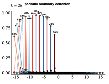
Refer to caption
Figure S5: Improving the “bond-dimension 2” multiparticle wavefunction by diagonalizing the projected Hamiltonian in the “variational subspace” {|Ξn|,n=113}\{|\Xi_{n}\rangle|,n=1\dots 13\}. Such procedure improves the approximations on the ground states and scar states near the ground state.

References