Pressure-Induced Metal-Insulator Transition in
Twisted Bilayer Graphene

Abstract

Recent experiments on twisted bilayer graphene (TBLG) have observed insulating states for two and three unit charges per moiré supercell, whereas the quarter–filling state (QFS) remained metallic. Subsequent experiments show that under hydrostatic pressure the QFS turns insulating for a certain window of pressure. In fact, the resistivity of the 1/2–filling and 3/4–filling states are also enhanced in the same pressure-window. Using pressure-dependent band structure calculations we compute the ratio of the potential to the kinetic energy, $r_{s}$. We find a window of pressure for which $r_{s}$ crosses the threshold for a triangular Wigner crystal, thereby corroborating our previous work that the insulating states in TBLG are driven by Wigner physics, A key prediction of this work is that the window for the onset of the hierarchy of Wigner states that obtains at commensurate fillings conforms to a dome shape under pressure. We also predict the optimal condition for Wigner crystallization to be around $1.5$ GPa. Consequently, TBLG provides a new platform for the exploration of Wigner physics and its relationship with superconductivity.

I Introduction

Twisted bi-layer graphene (TBLG) is a true example of emergence. Electrons in single layers of graphene are free while those in the composite consisting of two layers twisted close to the magic angle such that the electronic bands are essentially flat have almost no kinetic energy, $E_{K}$. In such cases, the physics is dominated by the interactions, $E_{U}$ , between the electrons. The experimental observation of correlated insulating phases and superconductivity is hence not unexpected. As a result of these discoveries Cao et al. (2018a, b), TBLG is largely viewed as a problem in strongly correlated physics Padhi et al. (2018); Xu et al. (2018); Irkhin and Skryabin (2018); Isobe et al. (2018); Liu et al. (2018); Ochi et al. (2018); Thomson et al. (2018); Dodaro et al. (2018); Xu and Balents (2018); Zou et al. (2018); Yuan and Fu (2018); Baskaran (2018); Koshino et al. (2018); Po et al. (2018); Kang and Vafek (2018); Po et al. ; Venderbos and Fernandes (2018). However, unlike conventional strongly correlated materials such as the cuprates or the heavy fermions, TBLG offers an extremely tunable platform. Namely, through the twist angle one can control the extent of strong correlation.

When two layers of graphene are rotated with respect to each other, a so called moiré lattice emerges Lopes dos Santos et al. (2012); Mele (2010); Lopes dos Santos et al. (2007); Bistritzer and MacDonald (2011), which is a triangular lattice with periodicity $\lambda_{s}=a/(2\sin\theta/2)$. Here $a=$2.46\text{\,}\mathrm{\SIUnitSymbolAngstrom}$$ is the lattice constant of pristine graphene layers. This emergent lattice has an approximate SU(4) symmetry due to the valley and spin degeneracies. Thus a moiré band can hold up to four electrons. So if we consider a moiré supercell of area $A_{s}=\sqrt{3}\lambda_{s}^{2}/2$, the superlattice density ($n_{s}$) can be fixed using $A_{s}n_{s}=4$. Consequently, it is convenient to define the index $\nu=n_{e}A_{s}$ which serves as the electron filling factor. The initial experiments Cao et al. (2018a, b) in this regime showed that insulating states can arise for $\nu=\pm 2,3$. Doping away from $\nu=-2$ resulted in superconductivity with a transition temperature of $1.5\,$K. These results were later confirmed by various groups Yankowitz et al. (2019); Kerelsky et al. ; Choi et al. ; Sharpe et al. ; Lu et al. ; Chen et al. . In particular, it was demonstrated  Yankowitz et al. (2019) that hydrostatic pressure can also be used to further tune the effects of twist angle. This gave way to certain metal–insulator and insulator–metal transitions which were not observed at ambient pressure. In this work we try to address the mechanism behind these peculiar transitions.

At zero temperature, a measure of the degree of correlation can be, $E_{U}/E_{K}\equiv r_{s}$. Starting from a two-dimensional homogenous gas of electrons (2DEG) one can drive the system through different phases simply by tuning $r_{s}$. This is true because the energy of a many-body ground state, $E_{0}(r_{s})$, is solely a function of $r_{s}$. The two asymptotic phases one thus obtains are a Fermi liquid phase for $r_{s}\lesssim 1$ and a Wigner solid phase Wigner (1934) for $r_{s}\gtrsim 37$ Tanatar and Ceperley (1989). Experimentally, in principle, one can access these phases by changing the carrier density ($n_{e}$) or applying a magnetic field ($B$). However, in the case of TBLG, $r_{s}$ can also be tuned by the twist angle ($\theta$) or hydrostatic pressure ($P$). At ambient pressure, a single layer of graphene Dahal et al. (2006) or a Bernal stacked bilayer of graphene Silvestrov and Recher (2017); Dahal et al. (2010) has $r_{s}\lesssim 1$. Twisting the layers towards a magic angle configuration increases $r_{s}$ of this TBLG system, driving it towards a Wigner phase Padhi et al. (2018). This can simply be understood by the flattening of the moiré bands. In fact, the proclivity of flat-band systems to form Wigner crystals has not gone unnoticed Wu et al. (2007). However, a natural question that arises is, how does pressure modulate $r_{s}$? To answer this question, we numerically compute $r_{s}$ of TBLG as a function of $\theta,n_{e},P$. With this we demonstrate that the metal–insulator–metal transition mentioned above can be understood as a melting of a Wigner solid phase; see Fig. 4.

This paper is organized in the following manner. In Sec. II we first argue that the correlated insulators observed in TBLG are Wigner, not Mott insulators. In Sec. III we discuss the tight-binding Hamiltonian we use for computing the band structure of TBLG. Pressure is then incorporated into computing the band structure in the presence of triangular warping, and a pressure-dependent effective magic angle is obtained in Sec. IV. We then proceed to compute pressure dependence of $r_{s}$ at various commensurate fillings in Sec. V. In Sec. VI we discuss a few possible corrections to our estimation of $r_{s}$. We conclude our discussion in Sec. VII by commenting on a few other aspects of TBLG in relation to Wigner crystals (WCs).

II TBLG: Mott versus Wigner Paradigm

This paper addresses the pressure dependence of the insulating states. Electronic band structure calculations Carr et al. (2018a); Fang and Kaxiras (2016); Lingam Chittari et al. (2019) as a function of pressure in TBLG offer immediate insight into the physics at play. Hydrostatic pressure causes uniaxial compression between the graphene layers Yankowitz et al. (2018), which in turn increases the interlayer tunneling, thereby changing the magic angle condition. However, an additional feature also appears: the bandwidth shows a dome-like shape with increasing pressure. Because the interactions remain fixed, the ratio $r_{s}$ increases, favoring Wigner crystallization. Although, simply from the bandwidth perspective, Mott insulation might also seem favorable.

It is important then to determine what physics TBLG exhibits that conforms to either scenario. Cao, et al. as well as others Xu and Balents (2018); Zou et al. (2018); Yuan and Fu (2018); Baskaran (2018) attributed the insulating states at $\nu=\pm 2,3$ to Mott physics. Within this paradigm, insulating behavior should exist whenever the band is partially filled. However, metallic not insulating behavior exists at $\nu=1$ in the experiments of Cao et al. (2018a, b). This is a potential problem for the application of the Mott scenario to TBLG. It is not surprising then that the Mott criterion Mott and Davis (2012) $n_{e}^{1/d}a_{0}^{\ast}\approx O(1)$ is not satisfied in TBLG near the magic angle. In fact, this is satisfied only for $\theta-\theta_{\rm magic}\gtrsim 0.7$.

Another key distinguishing feature between a Mott and a pinned Wigner insulator is that the spatial symmetry of the Mott state is always the same as that of the lattice. However, a Wigner crystal, being an emergent lattice by itself, may or may not adhere to the symmetries of the underlying lattice. Within the Mott paradigm, the relevant question is how can the electrons be placed in a moiré lattice without creating a new electron lattice distinct from the underlying triangular moiré lattice. That is, because of the Coulomb interaction, the electrons must occupy spatially separated locations in each moiré cell regardless of the underlying SU(4) symmetry. Consequently, except, for $\nu=1$, any arrangement of the electrons must create a lattice distinct from the triangular lattice. The honeycomb ($\nu=2$) (also proposed previously as a possible ground state Thomson et al. (2018); Xu et al. (2018)) and kagome ($\nu=3$) lattices are examples of Wigner lattices as they all break the underlying triangular symmetry Padhi et al. (2018). While the most common instances of Wigner crystal formation involve a magnetic field Monarkha and Syvokon (2012) that quenches the kinetic energy, the situation in TBLG is not very dis-similar because it is well known that a relative twist between two layers of graphene generates San-Jose et al. (2012) a non-Abelian gauge pseudo-potential Yin et al. (2015) with a magnetic length equal to the moiré lattice constant.

In the following sections we demonstrate that increasing the pressure in TBLG leads to $r_{s}>37$, thereby resolving the pressure-induced metal-insulator transition in TBLG. We map out the phase diagram using realistic parameters for TBLG and determine the regime where the $\nu=1$ state crosses the WC threshold. We find that the quarter-filling state in the new experiments Yankowitz et al. (2019) at $1.33$ and $2.21\,$GPa are well within the Wigner regime while those at ambient pressure correspond to $r_{s}<37$. We also confirm the experimental trend that hydrostatic pressure enhances the insulating states at $\nu=2,3$.

III The Tight–Binding Hamiltonian

We start by computing the pressure-dependent band structure and subsequently $r_{s}$. In our discussion, we will focus explicitly on device D2 of Yankowitz et al. (2019). Consider two layers of graphene, each rotated by $\pm\theta/2$ around an axis passing through an A₁B₂ site, where the subscripts denote the layers, and A, B are sublattice labels. When $\theta$ is small, the supercell consists of a large number of atoms, $\sim 10^{4}$, making ab initio methods Shallcross et al. (2008) less viable or reliable Trambly de Laissardiére et al. (2010) than the tight-binding schemes Lopes dos Santos et al. (2007, 2012). Here, we follow the tight-binding scheme of Carr et al. (2018a), where the tight-binding parameters are functions of pressure. Also, since we work with a tight-binding model, unlike the case of a continuum model, we limit our discussion to commensurate structures obtained for twist angles Shallcross et al. (2010),

$$\theta=\cos^{-1}\left[\frac{m^{2}+4mn+n^{2}}{2(m^{2}+mn+n^{2})}\right]\,,\quad m,n\in\mathrm{Z}\,.$$ (1)

The twist angle of the D2 sample is $\theta=$$$, which is not a commensurate angle. Because of the reasoning above, we work with the nearest commensurate angle, $\theta\approx$$$, obtained for $(m,n)=(26,27)$.

We denote the supercell vectors as $\boldsymbol{R}_{1}=m\boldsymbol{a}_{1}+n\boldsymbol{a}_{2}$ and $\boldsymbol{R}_{2}=-n\boldsymbol{a}_{1}+(m+n)\boldsymbol{a}_{2}$, with $\boldsymbol{a}_{1}$, $\boldsymbol{a}_{2}$ being the lattice vectors of original graphene layer, and each unit cell is $|m-n|$ ($=1$ for D2) times larger than the moiré periodicity, $\lambda_{s}$. For commensurate structures, there is a well defined moiré Brillouin zone (MBZ). The symmetry points of the MBZ will be labeled as $\bar{\Gamma}$ (zone center), $\rm\bar{M}$ (edge center), and $\rm\bar{K}$ (zone corner). Since tunneling between two valleys is prevented in a low-energy description ($\lesssim 1\;$eV) and as a result of the valley degeneracy, our calculation only considers an MBZ formed near the $\boldsymbol{K}$ (Dirac) point of the original lattice.

We begin with a simplified description, ignoring any angular dependence of the hybridization or the orbital overlaps. The generic non-interacting part of the Hamiltonian is

$$H=-\sum_{i,j}t(\boldsymbol{R}_{i}-\boldsymbol{R}_{j})\left\rvert\boldsymbol{R}_{i}\right\rangle\left\langle\boldsymbol{R}_{j}\right\rvert+\text{H.c.}\,,$$ (2)

where $\boldsymbol{R}_{i}=\sum_{x,y,z}{R_{i}}^{a}\,\boldsymbol{e}_{a}$ is the atomic coordinate in the basis of $\{\boldsymbol{e}_{a}\}$, and $\left\rvert\boldsymbol{R}_{i}\right\rangle$ is the wave function at site $i$. The tunneling strength between sites $i$ and $j$ is measured by the tight-binding parameter $t(\boldsymbol{R}_{i}-\boldsymbol{R}_{j})$. We can express this tight-binding parameter using a simple linear combination of $p_{z}$ orbitals as

$$t(\boldsymbol{R})=V_{pp\pi}(\boldsymbol{R})\,\sin^{2}\gamma+V_{pp\sigma}(\boldsymbol{R})\,\cos^{2}\gamma\,,$$ (3a)

$$R\cos\gamma=\boldsymbol{R}\cdot\boldsymbol{e}_{z}\,.$$ (3b)

Here $R$ is the length of the vector $\boldsymbol{R}$ joining two atoms and $\boldsymbol{e}_{z}$ is the unit vector along the $c$ axis. The overlap or transfer integrals, $V(\boldsymbol{R})$, can be expressed in terms of the Slater-Koster parameters Slater and Koster (1954)

$$V_{pp\pi}(\boldsymbol{R}) = -t_{0}\exp\left(-\frac{R-a_{0}}{r_{0}}\right)\,,$$ (4)

$$V_{pp\sigma}(\boldsymbol{R}) = t_{\perp}\exp\left(-\frac{R-d_{\perp}}{r_{0}}\right)\,.$$ (5)

$r_{0}=0.318\,a_{0}$ is an isotropic decay length chosen Trambly de Laissardiére et al. (2010) for the transfer integrals so that the next-nearest in-plane overlap becomes $0.1t_{0}$ Deacon et al. (2007). $t_{\perp}$ is the $\sigma$–bond (or interlayer coupling) strength between the $sp_{2}$ orbitals of the AB stacked bilayers. At ambient pressure $t_{\perp}|_{P=0}\equiv t^{0}_{\perp}\approx 0.31\,\rm eV$. $t_{0}\approx 2.7\;$eV is the in-plane $\pi$–bond strength of the two neighboring $p_{z}$ orbitals (separated by $a_{0}=a/\sqrt{3}=$1.42\text{\,}\mathrm{\SIUnitSymbolAngstrom}$$) in single-layer graphene. We use $d_{\perp}$ for the inter-layer spacing at finite pressure $P\,$(GPa) and $d_{\perp}^{\,0}=$3.35\text{\,}\mathrm{\SIUnitSymbolAngstrom}$$ is the spacing at ambient pressure.

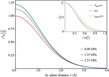
Figure 1: Inter-layer tunneling for different pressures as a function of distance from the site of rotation. With increasing pressure, the inter-layer distance decreases causing the tunneling strength to increase. Inset: The dominant contribution to $t(\boldsymbol{r})$ comes from $V_{pp\sigma}$ which leads to a simpler expression in Eq. (6).

Since $d_{\perp}/a_{0}\gtrsim 2$, near the stacking center, the tunneling parameter $t(\boldsymbol{R})$ is largely dominated by the $\sigma$ bond, and thus, the function $t(\boldsymbol{R})$ can be approximated as

$$t(\boldsymbol{r})\approx t_{\perp}\left(1-\frac{r^{2}}{d_{\perp}^{2}}\right)\exp\left(-\frac{r^{2}}{2r_{0}d_{\perp}}\right)\,.$$ (6)

In the inset of Fig. 1, the behavior of Eq. (6) is juxtaposed with the exact result from Eq. (3b), which shows an exponential reduction of the tunneling strength for $r\gtrsim d_{\perp}$. This also causes the Fourier transform to sharply decay for any $k\gtrsim 1/d_{\perp}$. Thus, for a low-energy model, it is sufficient to work with $t_{\perp}(\boldsymbol{K})$ only and not include the higher modes, such as $t_{\perp}(\boldsymbol{K}+\boldsymbol{G})$, where $\boldsymbol{G}$ is a moiré reciprocal lattice vector. One can perform a Fourier transform of $t(\boldsymbol{r})$ computed above to determine $t_{\perp}(\boldsymbol{K})$, or since we work in the $\theta\sim 1^{\circ}$ limit, (for AB stacking) one can approximate $t_{\perp}(\boldsymbol{K})/A_{0}\,\equiv w=\frac{1}{3}t_{\perp}\,.$ Here $A_{0}=\sqrt{3}a^{2}/2$ is the area of the single-layer graphene unit cell and the factor of $3$ takes into account that there are three equivalent Dirac cones. One can use $w$ as the input parameter in the effective theories.

In concluding this section we note that, in our discussion, $t_{\perp}$ is the single energy parameter that is affected by pressure [see Eq. (11)]. The in-plane energetics, controlled by in-plane hopping, may change under very high pressure, especially in the presence of a hexagonal boron nitride (hBN) substrate; however, for the range of pressure relevant here, such effects can be safely neglected Yankowitz et al. (2018).

IV Pressure Dependence of Magic Angle

In order to quantify the effect of pressure on $t_{\perp}$ first we need to obtain the relation between $d_{\perp}$ and pressure. Application of hydrostatic pressure can readily reduce $d_{\perp}$ Yankowitz et al. (2018), the experimental consequences of which have been studied in Yankowitz et al. (2019). This compression factor, denoted by $\delta_{d}$, is related to applied pressure through the Murnaghan equation of state Lingam Chittari et al. (2019)

$$1-\frac{d_{\perp}}{d_{\perp}^{\,0}}\equiv\delta_{d}=10.48\ln\left(1+\frac{P}{5.73}\right)\%\,.$$ (7)

The numbers appearing here are fixed using density functional theory Carr et al. (2018a). An immediate consequence of a reduced $d_{\perp}$ is an enhanced magic angle, which we denote by $\theta_{\text{\,magic}}^{\text{\,eff}}$. In fact, for experimentally accessible pressures, this mechanism can enhance $\theta_{\text{\,magic}}^{\text{\,eff}}$ up to $3\mathrm{°}$. The primary advantage of a large $\theta_{\text{\,magic}}^{\text{\,eff}}$ is an enhanced Coulomb energy scale ($E_{U}\sim\lambda_{\theta}^{-1}\sim\theta$) which could also result in an increased $T_{c}$ Yankowitz et al. (2019).

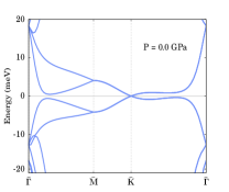
(a)

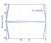
(b)

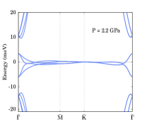
(c)

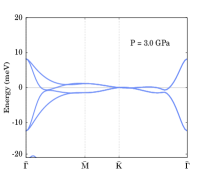
(d)

Figure 2: Pressure-dependent band dispersion of TBLG for $\theta=$$$. The parameters used in obtaining these are listed in the Table 1. With increasing pressure, the low energy bands become flatter; however, beyond $\sim 1.45\pm 0.1$ GPa, the bandwidth increases subsequently. The reason behind such an optimal behavior can be understood from Eq. (12).

In order to express $t(\boldsymbol{R})$ as a function of $\delta_{d}$ (hence, $P$), we use Eq. (7) in Eq. (5) or (6) and rewrite the tight-binding Hamiltonian. However, at finite pressure the Slater-Koster approximation turns contentious as the overlap between the Wannier orbitals develops a strong angular dependence Carr et al. (2018a); Fang and Kaxiras (2016); Lingam Chittari et al. (2019). This is a result of the overlap of Wannier orbitals with angular momentum, $m=3n$, with $n\in\mathbb{Z}$, where $3$ appears due to the $D_{3}$ point group symmetry of the underlying lattice. We will denote the radial components of such overlap functions with $V_{|m|}(r)$, whereas the angular dependence simply will be $\cos(m\theta)$. In this notation, Eq. (3b) can be viewed simply as $V_{0}(r)$, which still is the leading contribution to $t_{\perp}(\boldsymbol{r})$. In fact, we will only consider the overlaps from the $m=\pm 3,\pm 6$ orbitals since the effects from the overlap of the higher-order orbitals are negligible Fang and Kaxiras (2016). A real space expansion of $t_{\perp}(\boldsymbol{r})$ is thus written as Carr et al. (2018a); Fang and Kaxiras (2016); Lingam Chittari et al. (2019); Fang and Kaxiras (2016)

$$t_{\perp}(\boldsymbol{r})=V_{0}(r)+V_{3}(r)\left[\cos(3\theta_{12})+\cos(3\theta_{21})\right]$$

$$+V_{6}(r)\left[\cos(6\theta_{12}+\cos(6\theta_{21}))\right]\,,$$ (8)

where $\theta_{ij}$ are the angles between the vectors connecting the $i\textsuperscript{th}$ site to the $j\textsuperscript{th}$ site and that connecting the $i\textsuperscript{th}$ site to its nearest neighbor. The radial functions $V_{|m|}(r)$ are given by

$$V_{0}(r) =\lambda_{0}e^{-\xi_{0}\bar{r}^{2}}\cos(\kappa_{0}\bar{r})\,,$$ (9a)

$$V_{3}(r) =\lambda_{3}\bar{r}^{2}e^{-\xi_{3}(\bar{r}-x_{3})^{2}}\,,$$ (9b)

$$V_{6}(r) =\lambda_{6}e^{-\xi_{6}(\bar{r}-x_{6})^{2}}\sin(\kappa_{6}\bar{r})\,.$$ (9c)

Here $\bar{r}=r/a$. All the parameters appearing above, collectively denoted by $\pi_{i}(\delta_{d})$ where $i=1,2,\cdots 10$, are fixed Carr et al. (2018a) using density functional methods and are listed in the Table 1. Given the pressure range of interest, the functional dependence of $\pi_{i}(\delta_{d})$ with $\delta_{d}$ is truncated to a quadratic fit

$$\pi_{i}(\delta_{d})=c_{i}^{(0)}-c_{i}^{(1)}\delta_{d}+c_{i}^{(2)}\delta_{d}^{2}\,.$$ (10)

$i\,(\pi_{i})$	$c_{i}^{(0)}$	$c_{i}^{(1)}$	$c_{i}^{(2)}$
$1\,(\lambda_{0})$	$\phantom{-}0.310$	$-1.882$	$\phantom{-}7.741$
$2\,(\xi_{0})$	$\phantom{-}1.750$	$-1.618$	$\phantom{-}1.848$
$3\,(\kappa_{0})$	$\phantom{-}1.990$	$\phantom{-}1.007$	$\phantom{-}2.427$
$4\,(\lambda_{3})$	$-0.068$	$\phantom{-}0.399$	$-1.739$
$5\,(\xi_{3})$	$\phantom{-}3.286$	$-0.914$	$\phantom{-}12.011$
$6\,(x_{3})$	$\phantom{-}0.500$	$\phantom{-}0.322$	$\phantom{-}0.908$
$7\,(\lambda_{6})$	$-0.008$	$\phantom{-}0.046$	$-0.183$
$8\,(\xi_{6})$	$\phantom{-}2.272$	$-0.721$	$-4.414$
$9\,(x_{6})$	$\phantom{-}1.217$	$\phantom{-}0.027$	$-0.658$
$10\,(\kappa_{6})$	$\phantom{-}1.562$	$-0.371$	$-0.134$

Table 1: Compression, $\delta_{d}$, dependence of the ten-parameters appearing in Eq. (9). The coefficients, $c_{i}^{(n)}$, appearing in Eq. (10) are listed below (in eV units). The theory for determining these coefficients was developed in Refs. Fang and Kaxiras (2016); Carr et al. (2018a).

For numerical accuracy, our band structure computations are based on this full ten-parameter model (see Fig. 2); however, for simplicity, henceforth we confine our discussion to an effective one-parameter model. In Eq. (9) the strongest contributions to the interlayer tunneling come from the hybridization scales $\lambda_{i}$. The remaining parameters, the length scales associated with the Wannier orbitals, are weakly dependent on pressure. Thus, a simpler effective model could be constructed by renormalizing these three parameters (first row of Table 1), where the renormalization essentially takes into account the angular contributions coming from all the other parameters (the remaining nine rows in Table 1). Such an effective set of parameters was obtained in Carr et al. (2018a) by tallying the bandwidth of the flat bands from the ten-parameter model and an ab initio $k\cdot p$ model

$$t_{\perp}(\delta_{d})=t_{\perp}^{(0)}-t_{\perp}^{(1)}\delta_{d}+t_{\perp}^{(2)}\delta_{d}^{2}\quad,\quad$$

$$t_{\perp}^{(0,1,2)}\simeq(0.31,-1.73,7.12)\;\text{eV}\,.$$ (11)

Again, the parameters $t_{\perp}^{(i)}$s above, which marginally differ from those listed in the first row of Table 1, can be simply seen as effective leading parameters after incorporating the angular contributions. Note that the above $t_{\perp}$, thus constructed, is the single input to the tight-binding Hamiltonian of the previous section. Now, however, it is dependent on pressure.

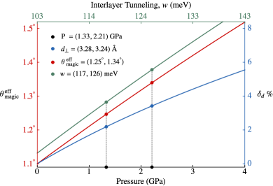
Figure 3: With increasing external pressure, the inter-layer distance decreases by $\delta_{d}\%$ (blue curve or right axis) which is described in Eq. (7). Reduced separation enhances inter-layer tunneling, $w\approx t_{\perp}/3$ (green curve or top axis), as can be seen from Eq. (11). This causes an increase (red curve or left axis) in the effective magic angle, $\theta_{\text{\,magic}}^{\text{\,eff}}$, where the band become the flattest, see Eq. (12). The dots correspond to the reported values of pressure where the measurements of Yankowitz et al. (2019) were performed.

Using Eq. (11), we now obtain the pressure dependence of $\theta_{\text{\,magic}}^{\text{\,eff}}$ discussed before. Note that the magic angle is (roughly) obtained by matching the quasiparticle kinetic energy, $\hbar v_{0}K_{\theta}$, and the hybridization scale, $t_{\perp}$. Here $v_{0}=10^{6}\,$m/s is the speed of the electrons in pristine graphene and $K_{\theta}=4\pi/3\lambda_{s}$ is the size of the MBZ. This causes $\theta_{\text{\,magic}}^{\text{\,eff}}\sim t_{\perp}$, or, at ambient pressure, $\theta_{\rm magic}\sim t_{\perp}^{(0)}$. Thus, $\hbar v_{0}K_{\theta}=\theta_{\text{\,magic}}^{\text{\,eff}}\left(2t_{\perp}^{(0)}/\theta_{\text{magic}}\right)$. Following Carr et al. (2018a); Lingam Chittari et al. (2019); Yankowitz et al. (2019), we set $\theta_{\text{magic}}=$$$. This gives rise to the following expression for the effective magic angle

$$\frac{\theta_{\text{\,magic}}^{\text{\,eff}}(P)}{\theta_{\text{\,magic}}}=\frac{t_{\perp}(P)}{t_{\perp}^{0}}=1+5.584\,\delta_{d}+22.97\,\delta_{d}^{2}\,.$$ (12)

Figure 3 displays the relevant parameters discussed above as functions of external pressure. For a given device with a fixed twist angle $\theta$, which is larger than the ambient pressure magic angle $\theta_{\text{magic}}$, as pressure increases one gradually increases $\theta_{\text{\,magic}}^{\text{\,eff}}$. For $\theta=\theta_{\text{\,magic}}^{\text{\,eff}}$, one defines the optimum pressure for a particular system, $P_{\rm opt}$ , which is also coincident with the flat-band condition. Increasing the pressure further will relatively tune the system away from the magic angle. The optimal pressure for device D2, for instance, can be solved by demanding $\theta_{\text{\,magic}}^{\text{\,eff}}=$$$. From Eq. (12), we find that $P\simeq 1.55$ GPa ($\delta_{d}=2.5\,\%$). This explains why optimal behavior is seen (among the two available data sets) around $1.33$ GPa ($\delta_{d}=2.2\,\%$), as opposed to near $2.21$ GPa ($\delta_{d}=3.4\,\%$).

With the use of these parameters, we compute the band structure. The most notable feature in Fig. 2 is that the bandwidth shrinks as $1.33\,$GPa is approached and increases beyond this pressure. It is this feature that gives rise to the dome-like shape of the phase diagram of $r_{s}$ versus hydrostatic pressure, thereby affecting the observed insulating behavior. Note that, although here we used the tight-binding description, one may also use the effective low energy descriptions developed for ambient pressure Bistritzer and MacDonald (2011); Yuan and Fu (2018); Koshino et al. (2018); Po et al. (2018); Kang and Vafek (2018); Po et al. ; albeit the (tight-binding or continuum) parameters must be fixed taking finite pressure into account.

V Computation of $r_{s}$

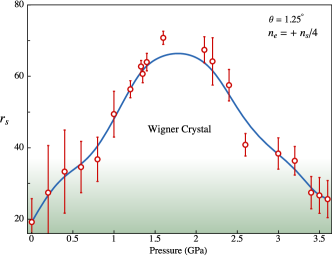
Figure 4: For the device D2 of Yankowitz et al. (2019), we compute $r_{s}$ (red dots along with computational error associated with coarse graining of the $k$ space) of the quarter-filling state. The blue curve provides a guide for the eye. Its dome-like behavior can explain a similar feature seen in the conductance of the quarter-filling state in the experiment of Yankowitz et al. (2019). For the pressure window of $\sim 1-3$ GPa the system enters the Wigner crystallization regime, $r_{s}\gtrsim 37$. Similar behavior is obtained for $n_{e}=n_{s}/2$ and $3n_{s}/4$.

We now turn to the computation of $r_{s}$. First we need to estimate Coulomb energy for a TBLG system at $\theta$ angle,

$$E_{U}=\frac{e^{2}}{\epsilon r_{e}}=\left(\frac{\alpha}{\epsilon}\right)\left(\frac{\hbar v_{0}}{a}\right)\left(\frac{a}{r_{e}}\right)\,.$$ (13)

Since $v_{0}$ is about $300$ times smaller than the speed of light, the effective fine structure constant of (suspended) graphene is $\alpha\approx 2.2$. Also note that $\hbar v_{0}/a=2.135\;$eV. In the presence of the hBN substrate, this is reduced by a factor of the effective dielectric constant, $\epsilon=10$ . The average inter-particle distance can be obtained from $\pi r_{e}^{2}n_{e}=1$. For a given filling fraction, $r_{e}=\sqrt{A_{s}/\pi\nu}\approx{0.525}\,\lambda_{s}/\sqrt{\nu}$. Combining all of these expressions, we find that $E_{U}\approx(15\;\text{meV})\,\theta^{\,\circ}$. In Sec. VI we discuss some subtleties involved with a more realistic estimation of $E_{U}$ in TBLG. The final expression for $r_{s}$ is

$$r_{s}\approx 15\,\text{meV}\,\frac{\theta^{\,\circ}}{E_{K}}\,\sqrt{\nu}\xrightarrow[\text{D2}]{\text{Device}}\,\frac{20\,\text{meV}}{E_{K}\,(\text{meV})}\,\sqrt{\nu}\,.$$ (14)

In order to fix the kinetic energy above, we first relate the carrier concentration to chemical potential, $\mu$, and since $E_{K}\lesssim\mu$, for a minimal (and hence conservative) estimate of $r_{s}$, one can substitute $E_{K}$ with $\mu$. In order to do so we start by computing the density of states (DOS), $\rho(\epsilon)$, which can be normalized in the following way. Since each moiré supercell contains eight electrons at the most, integrating the DOS for the bottom four bands must yield $8$

$$\int_{\Lambda_{h}}^{\Lambda_{e}}\rho(\epsilon)d\epsilon=8\,.$$ (15)

Here, $\Lambda_{e,h}\sim\pm 10\,\rm meV$, respectively, provide the upper and lower cutoff for the bottom four bands. Integrating the normalized DOS up to the chemical potential provides the carrier concentration (in order to compare our results with those of  Yankowitz et al. (2019) we do so for the hole side):

$$n_{e}(\mu)=\int_{\Lambda_{h}}^{\mu}\rho(\epsilon)d\epsilon\,.$$ (16)

This is shown in Fig. 5a. In obtaining $r_{s}$ for the $\nu/4$ state one can fix $n_{e}(\mu)=\nu\,n_{s}/4$ (e.g., see the gray line for $\nu=1$) and obtain how $\mu$ evolves with pressure along that line. Note the source of error here is the coarse graining of the energy integral above.

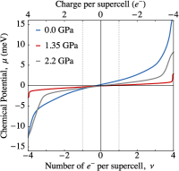
(a)

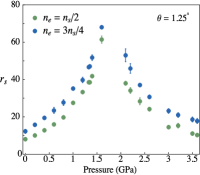
(b)

Figure 5: (a) The chemical potential dependence (smoothly fitted) of the carrier concentration for various pressures, as obtained in Eq. (16). (b) $r_{s}$ as a function of pressure obtained for $\nu=2,3$ states. Similar to the $\nu=1$ state discussed in the main text they also exhibit dome–like behavior.

In Fig. 4 [or Fig. 5b] we plot the behavior of $r_{s}$ as a function of pressure, which is clearly dome-like. The key aspect of this figure is the crossing of the Wigner threshold for pressures in the range $0.75<P<3$ GPa. The existence of this window for optimal insulating behavior of the $\nu=1$ state can be tested experimentally. We find that $P_{opt}=1.5$ GPa, which is close to the experimentally observed optimal pressure, $1.33$ GPa. Clearly further experiments are needed to map out the non-monotonic dependence of the metal-insulator transition as a function of the uniaxial pressure. As can be seen in Fig. 5b, similar behavior is seen for the $\nu=2,3$ states, which, as we showed previously Padhi et al. (2018), correspond to honeycomb and kagome Wigner crystals.

VI Possible Sources of Corrections to $r_{s}$

There are several variables present in a realistic hBN-TBLG system which might affect the exactness of our estimated $r_{s}$. In this section we list numerous such effects and discuss their consequences. We argue that these variables do not influence the order of our estimations significantly nor do they alter our qualitative conclusions. Hence, for simplicity, we have not considered them in our estimation.

Before turning to a discussion pertaining to TBLG we first note that the critical value for Wigner crystallization used in this work, $r^{\rm crit}_{s}=37$, though universal across all materials, is somewhat approximate. The computational sources of error are the finite-size effect (extrapolation of finite number of electrons to the thermodynamic limit), and the fitting errors in obtaining $E_{0}(r_{s})$. Cumulatively, they amount to an error of magnitude $\delta r^{\rm crit}_{s}=5$ in Tanatar and Ceperley (1989). Another important source of uncertainty in $r_{s}^{\rm crit}$ is a methodical error arising from the so-called fixed-node approximation used in the diffusion Monte Carlo method Anderson (1976) (that the actual and the trial wave functions share the same nodal surface). An improved use of this approximation was done in Drummond and Needs (2009) by including Slater-Jastrow-backflow wave functions López Ríos et al. (2006). This results in $r_{s}^{\rm crit}=31\pm 1$, which incidentally lowers (raises) the critical pressure at which the metal to insulator (insulator to metal) transition occurs; see Fig. 4. However, it should also be noted that the transition in Drummond and Needs (2009) is from a paramagnetic fluid to a triangular antiferromagnetic crystal, as opposed to a transition from a ferromagnetic fluid to the triangular ferromagnetic crystal as reported in Tanatar and Ceperley (1989). In view of all these uncertainties the phase boundary in Fig. 4 remains intact.

In our work we have ignored any effects related to atomic relaxation in TBLG. For instance, the optimal lattice configuration of TBLG with twist angle $\lesssim 2^{\circ}$ is corrugated along the $c$ axis Uchida et al. (2014). This causes the inter-layer separation $d_{\perp}$ (or the inter-layer coupling $w$) to increase (reduce) in the AA-stacking region and decrease (enhance) in the AB/BA-stacking region. The consequences of such an effect on the band structure of near-magic-angle TBLG is that Koshino et al. (2018); Carr et al. (2018a) corrugation significantly enhances the band gap between the moireé flat bands and the higher-energy bands, albeit leaving the bandwidth virtually unchanged. Thus, as the bandwidth sets the scale for the kinetic energy as an input into the computation of $r_{s}$, the effect of out-of-plane relaxation is negligible in our case. Enhancement of the band gap simply strengthens the assumption of the flat bands being isolated.

In-plane relaxation effects often shrink the area of the AA-stacking region, concomitantly facilitating formation of a triangular domain structure with alternating AB- and BA-stacking regions Nam and Koshino (2017). In this case as well, the band gap increases; however, unlike the earlier case, in-plane relaxations cause the bandwidth to increase, though no more than $10\%$ at ambient pressure. Naively this should also lower our estimations of $r_{s}(P=0)$ by a similar fraction. However, to the best of our knowledge, the full inclusion of all the relaxation effects (see Carr et al. (2018b)), let alone with pressure dependence, has not yet been studied in detail. Thus, for simplicity we ignore any such effects in this work, which can at most change our estimates by 10$\%$.

It must also be noted that most of the near-magic-angle devices suffer from a twist angle inhomogeneity Kerelsky et al. ; Beechem et al. (2014); Yoo et al. which often has dramatic consequences on the phase diagram of TBLG Lu et al. . In other words, the local modulation in the twist angle could render $r_{s}$ to be a position-dependent function. Thus, it is perfectly possible that the sample as a whole may not undergo crystallization transition but it could form puddles of WCs, phase separated with other insulating or metallic states. Such consideration often plays a key role in experimental observation of WCs Martin et al. (2008).

In all of our calculations, the presence of the hBN layer(s) is accounted for only through the dielectric constant. However, the alignment or misalignment of the hBN substrate with the adjacent graphene layer of TBLG could significantly influence the phase diagram. Most importantly, the appearance or enhancement of a band gap near the Dirac point could Song et al. (2013); Jung et al. (2015) primarily emerge from moiré patterns or strains in the bilayer formed out of hBN/graphene Jung et al. (2017). Clearly, such an effect mainly drives the physics near charge neutrality. For instance, the appearance of a superconducting dome near charge neutrality in Lu et al. could possibly be attributed to the physics of hBN/graphene bilayer. Thus, for the bulk of our interest such an effect does not contribute to $r_{s}$.

VII Concluding Remarks

We have shown that the pressure dependence of the metal-insulator transition has a natural explanation within the hierarchy of Wigner crystals proposed recently for TBLG Padhi et al. (2018). Should the dome-like phase diagram for the $\nu=1$ state be confirmed experimentally, then this would add significant substantiation to the claim that TBLG offers a playground for observing WCs and the possible onset of superconductivity.

Our proposal that superconductivity lurks in the vicinity of Wigner crystallization is rooted in the retardation effects that are inherent to the strongly correlated regime. From the potential of interaction of an electron in a Wigner crystal Takada (1993),

$$V({\bf r})=-\frac{3}{2}\frac{e^{2}}{a^{\ast}r_{s}}+\frac{1}{2}\frac{e^{2}}{(a^{\ast}r_{s})^{3}}{\bf r}^{2}=-\frac{3}{2}\frac{e^{2}}{a^{\ast}r_{s}}+\frac{1}{2}\omega^{2}{\bf r}^{2},$$ (17)

increasing the electron density decreases the restoring frequency, $\omega$, thereby leading to a melting of a WC. However, when a charge moves in a WC, it must dissociate from the Coulomb or correlation hole that led to the formation of the crystal in the first place. The size of this correlation hole is $r_{e}$ and hence is roughly 10, 000 carbon atoms in TBLG at the relevant magic angles. Such a correlation hole and the electrons move on different time scales. Once the crystal moves, the correlation hole left behind is now positively charged and hence, on the timescale that it is vacated, it is attractive to the electrons in its vicinity. Consequently, such charge retardation effects could mediate pairing. This is the purely electron analog of the polaron effect and has been proposed previously to mediate pairing in the vicinity of the melting transition of Wigner crystals Phillips et al. (1998); Takada (1993); Bianconi and Missori (1994). Of course the form of the kinetic energy term will have to be modified for TBLG but the content of the argument remains intact. We hope to address this issue in greater detail in future work.

Regarding the spin dependence of the insulating states, the ferromagnetic triangular WC is well known Tanatar and Ceperley (1989) to be energetically favored for the $\nu=1$ state. The honeycomb WC we proposed has explicitly two electrons residing in each moiré cell and hence has $S=0$. The spin structure of the kagome lattice has no natural singlet correlations and hence should be spin-polarized just as in the $\nu=1$ case. Hence, we anticipate for $\nu=3$ the ground state is a ferromagnet, as has been observed recently Sharpe et al. . Previously, ferromagnetic Wigner crystallization has been used to explain the $1/6$-th filling-state in graphyne Chen et al. (2018). Within a Mott scenario, it is difficult to explain the spin dependence without at the same time invoking sites for the spins which would make the resultant electron lattice distinct from the underlying triangular moiré lattice. Recall, a Mott insulator cannot break any underlying symmetries. In this regard, the $1/2$-filled honeycomb structures proffered Thomson et al. (2018); Xu et al. (2018) to explain the $\nu=1/2$ states are instances of the WC we have proposed here. Consequently, all the features of the novel insulating states in TBLG are captured by a transition to WC.

It must also be noted that in our proposal, unlike the case of GaAs/AlGaAs heterostructures Kravchenko and Sarachik (2003) or that of liquid helium Grimes and Adams (1979), there is a WC pinned to the underlying moiré lattice. This poses a unique set of experimental challenges in distinguishing it from a Mott (or any other correlated) insulator Dobrosavljevic et al. (2012); Camjayi et al. (2008). For instance, formation of a WC, particularly adjacent to a gapped state, is often signaled by an instability in the thermodynamic compressibility Eisenstein et al. (1992). Thus far, similar measurements in TBLG Tomarken et al. observe phases with nondiverging and non-negative compressibility at commensurate fillings. Although one cannot rule out the influence of (twist or charge) disorder, strong pinning of the Wigner lattice to the moiré lattice may also render the insulating states incompressible Padhi et al. (2019). Consequently, the precise conclusion to be drawn from the compressibility experiments remains unclear at present.

References

- Cao et al. (2018a) Yuan Cao, Valla Fatemi, Ahmet Demir, Shiang Fang, Spencer L Tomarken, Jason Y Luo, Javier D Sanchez-Yamagishi, Kenji Watanabe, Takashi Taniguchi, Efthimios Kaxiras, Ray C. Ashoori, and Pablo Jarillo-Herrero, “Correlated insulator behaviour at half-filling in magic-angle graphene superlattices,” Nature 556, 80 (2018a).
- Cao et al. (2018b) Yuan Cao, Valla Fatemi, Shiang Fang, Kenji Watanabe, Takashi Taniguchi, Efthimios Kaxiras, and Pablo Jarillo-Herrero, “Unconventional superconductivity in magic-angle graphene superlattices,” Nature 556, 43 (2018b).
- Padhi et al. (2018) Bikash Padhi, Chandan Setty, and Philip W. Phillips, “Doped twisted bilayer graphene near magic angles: Proximity to wigner crystallization, not mott insulation,” Nano Letters 18, 6175–6180 (2018).
- Xu et al. (2018) Xiao Yan Xu, K. T. Law, and Patrick A. Lee, “Kekulé valence bond order in an extended hubbard model on the honeycomb lattice with possible applications to twisted bilayer graphene,” Phys. Rev. B 98, 121406 (2018).
- Irkhin and Skryabin (2018) V Yu Irkhin and Yu N Skryabin, “Dirac points, spinons and spin liquid in twisted bilayer graphene,” JETP Letters , 1–4 (2018).
- Isobe et al. (2018) Hiroki Isobe, Noah F. Q. Yuan, and Liang Fu, “Unconventional superconductivity and density waves in twisted bilayer graphene,” Phys. Rev. X 8, 041041 (2018).
- Liu et al. (2018) Cheng-Cheng Liu, Li-Da Zhang, Wei-Qiang Chen, and Fan Yang, “Chiral sdw and d+ id superconductivity in the magic-angle twisted bilayer-graphene,” arXiv:1804.10009 (2018).
- Ochi et al. (2018) Masayuki Ochi, Mikito Koshino, and Kazuhiko Kuroki, “Possible correlated insulating states in magic-angle twisted bilayer graphene under strongly competing interactions,” Phys. Rev. B 98, 081102 (2018).
- Thomson et al. (2018) Alex Thomson, Shubhayu Chatterjee, Subir Sachdev, and Mathias S. Scheurer, “Triangular antiferromagnetism on the honeycomb lattice of twisted bilayer graphene,” Phys. Rev. B 98, 075109 (2018).
- Dodaro et al. (2018) J. F. Dodaro, S. A. Kivelson, Y. Schattner, X. Q. Sun, and C. Wang, “Phases of a phenomenological model of twisted bilayer graphene,” Phys. Rev. B 98, 075154 (2018).
- Xu and Balents (2018) Cenke Xu and Leon Balents, “Topological superconductivity in twisted multilayer graphene,” Phys. Rev. Lett. 121, 087001 (2018).
- Zou et al. (2018) Liujun Zou, Hoi Chun Po, Ashvin Vishwanath, and T. Senthil, “Band structure of twisted bilayer graphene: Emergent symmetries, commensurate approximants, and wannier obstructions,” Phys. Rev. B 98, 085435 (2018).
- Yuan and Fu (2018) Noah F. Q. Yuan and Liang Fu, “Model for the metal-insulator transition in graphene superlattices and beyond,” Phys. Rev. B 98, 045103 (2018).
- Baskaran (2018) Ganapathy Baskaran, “Theory of emergent josephson lattice in neutral twisted bilayer graphene (moiré is different),” arXiv:1804.00627 (2018).
- Koshino et al. (2018) Mikito Koshino, Noah F. Q. Yuan, Takashi Koretsune, Masayuki Ochi, Kazuhiko Kuroki, and Liang Fu, “Maximally localized wannier orbitals and the extended hubbard model for twisted bilayer graphene,” Phys. Rev. X 8, 031087 (2018).
- Po et al. (2018) Hoi Chun Po, Liujun Zou, Ashvin Vishwanath, and T. Senthil, “Origin of Mott Insulating Behavior and Superconductivity in Twisted Bilayer Graphene,” Physical Review X 8, 031089 (2018).
- Kang and Vafek (2018) Jian Kang and Oskar Vafek, “Symmetry, maximally localized wannier states, and a low-energy model for twisted bilayer graphene narrow bands,” Phys. Rev. X 8, 031088 (2018).
- (18) H. C. Po, L. Zou, T. Senthil, and A. Vishwanath, “Faithful Tight-binding Models and Fragile Topology of Magic-angle Bilayer Graphene,” arXiv:1808.02482 .
- Venderbos and Fernandes (2018) Jörn W. F. Venderbos and Rafael M. Fernandes, “Correlations and electronic order in a two-orbital honeycomb lattice model for twisted bilayer graphene,” Phys. Rev. B 98, 245103 (2018).
- Lopes dos Santos et al. (2012) J. M. B. Lopes dos Santos, N. M. R. Peres, and A. H. Castro Neto, “Continuum model of the twisted graphene bilayer,” Phys. Rev. B 86, 155449 (2012).
- Mele (2010) E. J. Mele, “Commensuration and interlayer coherence in twisted bilayer graphene,” Phys. Rev. B 81, 161405 (2010).
- Lopes dos Santos et al. (2007) J. M. B. Lopes dos Santos, N. M. R. Peres, and A. H. Castro Neto, “Graphene bilayer with a twist: Electronic structure,” Phys. Rev. Lett. 99, 256802 (2007).
- Bistritzer and MacDonald (2011) Rafi Bistritzer and Allan H. MacDonald, “Moiré bands in twisted double-layer graphene,” Proceedings of the National Academy of Sciences 108, 12233–12237 (2011).
- Yankowitz et al. (2019) Matthew Yankowitz, Shaowen Chen, Hryhoriy Polshyn, Yuxuan Zhang, K. Watanabe, T. Taniguchi, David Graf, Andrea F. Young, and Cory R. Dean, “Tuning superconductivity in twisted bilayer graphene,” Science 363, 1059–1064 (2019).
- (25) Alexander Kerelsky, Leo McGilly, Dante M. Kennes, Lede Xian, Matthew Yankowitz, Shaowen Chen, K. Watanabe, T. Taniguchi, James Hone, Cory Dean, Angel Rubio, and Abhay N. Pasupathy, “Magic Angle Spectroscopy,” arXiv:1812.08776 [cond-mat.mes-hall] .
- (26) Youngjoon Choi, Jeannette Kemmer, Yang Peng, Alex Thomson, Harpreet Arora, Robert Polski, Yiran Zhang, Hechen Ren, Jason Alicea, Gil Refael, Felix von Oppen, Kenji Watanabe, Takashi Taniguchi, and Stevan Nadj-Perge, “Imaging Electronic Correlations in Twisted Bilayer Graphene near the Magic Angle,” arXiv:1901.02997 [cond-mat.mes-hall] .
- (27) Aaron L. Sharpe, Eli J. Fox, Arthur W. Barnard, Joe Finney, Kenji Watanabe, Takashi Taniguchi, M. A. Kastner, and David Goldhaber-Gordon, “Emergent ferromagnetism near three-quarters filling in twisted bilayer graphene,” arXiv:1901.03520 [cond-mat.mes-hall] .
- (28) Xiaobo Lu, Petr Stepanov, Wei Yang, Ming Xie, Mohammed Ali Aamir, Ipsita Das, Carles Urgell, Kenji Watanabe, Takashi Taniguchi, Guangyu Zhang, Adrian Bachtold, Allan H. MacDonald, and Dmitri K. Efetov, “Superconductors, Orbital Magnets, and Correlated States in Magic Angle Bilayer Graphene,” 1903.06513 [cond-mat.str-el] .
- (29) Guorui Chen, Aaron L. Sharpe, Patrick Gallagher, Ilan T. Rosen, Eli Fox, Lili Jiang, Bosai Lyu, Hongyuan Li, Kenji Watanabe, Takashi Taniguchi, Jeil Jung, Zhiwen Shi, David Goldhaber- Gordon, Yuanbo Zhang, and Feng Wang, “Signatures of Gate-Tunable Superconductivity in Trilayer Graphene/Boron Nitride Moir\’e Superlattice,” arXiv:1901.04621 [cond-mat.supr-con] .
- Wigner (1934) E. Wigner, “On the interaction of electrons in metals,” Phys. Rev. 46, 1002–1011 (1934).
- Tanatar and Ceperley (1989) B. Tanatar and D. M. Ceperley, “Ground state of the two-dimensional electron gas,” Phys. Rev. B 39, 5005–5016 (1989).
- Dahal et al. (2006) Hari P. Dahal, Yogesh N. Joglekar, Kevin S. Bedell, and Alexander V. Balatsky, “Absence of wigner crystallization in graphene,” Phys. Rev. B 74, 233405 (2006).
- Silvestrov and Recher (2017) P. G. Silvestrov and P. Recher, “Wigner crystal phases in bilayer graphene,” Phys. Rev. B 95, 075438 (2017).
- Dahal et al. (2010) Hari P. Dahal, Tim O. Wehling, Kevin S. Bedell, Jian-Xin Zhu, and A.V. Balatsky, “Charge inhomogeneity in a single and bilayer graphene,” Physica B: Condensed Matter 405, 2241 – 2244 (2010).
- Wu et al. (2007) Congjun Wu, Doron Bergman, Leon Balents, and S. Das Sarma, “Flat bands and wigner crystallization in the honeycomb optical lattice,” Phys. Rev. Lett. 99, 070401 (2007).
- Carr et al. (2018a) Stephen Carr, Shiang Fang, Pablo Jarillo-Herrero, and Efthimios Kaxiras, “Pressure dependence of the magic twist angle in graphene superlattices,” Phys. Rev. B 98, 085144 (2018a).
- Fang and Kaxiras (2016) Shiang Fang and Efthimios Kaxiras, “Electronic structure theory of weakly interacting bilayers,” Phys. Rev. B 93, 235153 (2016).
- Lingam Chittari et al. (2019) Bheema Lingam Chittari, Nicolas Leconte, Srivani Javvaji, and Jeil Jung, “Pressure induced compression of flatbands in twisted bilayer graphene,” Electronic Structure 1, 015001 (2019).
- Yankowitz et al. (2018) Matthew Yankowitz, Jeil Jung, Evan Laksono, Nicolas Leconte, Bheema L. Chittari, K. Watanabe, T. Taniguchi, Shaffique Adam, David Graf, and Cory R. Dean, “Dynamic band-structure tuning of graphene moiré superlattices with pressure,” Nature (London) 557, 404–408 (2018).
- Mott and Davis (2012) Nevill Francis Mott and Edward A Davis, Electronic processes in non-crystalline materials (OUP Oxford, 2012).
- Monarkha and Syvokon (2012) Yu. P. Monarkha and V. E. Syvokon, “A two-dimensional wigner crystal (review article),” Low Temperature Physics 38, 1067–1095 (2012).
- San-Jose et al. (2012) P. San-Jose, J. González, and F. Guinea, “Non-abelian gauge potentials in graphene bilayers,” Phys. Rev. Lett. 108, 216802 (2012).
- Yin et al. (2015) Long-Jing Yin, Jia-Bin Qiao, Wei-Jie Zuo, Wen-Tian Li, and Lin He, “Experimental evidence for non-abelian gauge potentials in twisted graphene bilayers,” Phys. Rev. B 92, 081406 (2015).
- Shallcross et al. (2008) S. Shallcross, S. Sharma, and O. A. Pankratov, “Quantum interference at the twist boundary in graphene,” Phys. Rev. Lett. 101, 056803 (2008).
- Trambly de Laissardiére et al. (2010) G. Trambly de Laissardiére, D. Mayou, and L. Magaud, “Localization of dirac electrons in rotated graphene bilayers,” Nano Letters 10, 804–808 (2010).
- Shallcross et al. (2010) S. Shallcross, S. Sharma, E. Kandelaki, and O. A. Pankratov, “Electronic structure of turbostratic graphene,” Phys. Rev. B 81, 165105 (2010).
- Slater and Koster (1954) J. C. Slater and G. F. Koster, “Simplified lcao method for the periodic potential problem,” Phys. Rev. 94, 1498–1524 (1954).
- Deacon et al. (2007) R. S. Deacon, K.-C. Chuang, R. J. Nicholas, K. S. Novoselov, and A. K. Geim, “Cyclotron resonance study of the electron and hole velocity in graphene monolayers,” Phys. Rev. B 76, 081406 (2007).
- (49) J. M. Pizarro, M. Rösner, R. Thomale, R. Valentí, and T. O. Wehling, “Internal screening and dielectric engineering in magic-angle twisted bilayer graphene,” arXiv e-prints arXiv:1904.11765 [cond-mat.str-el] .
- Anderson (1976) James B. Anderson, “Quantum chemistry by random walk. h 2p, h+3 d3h 1a′1, h2 3Σ+u, h4 1Σ+g, be 1s,” The Journal of Chemical Physics 65, 4121–4127 (1976).
- Drummond and Needs (2009) N. D. Drummond and R. J. Needs, “Phase diagram of the low-density two-dimensional homogeneous electron gas,” Phys. Rev. Lett. 102, 126402 (2009).
- López Ríos et al. (2006) P. López Ríos, A. Ma, N. D. Drummond, M. D. Towler, and R. J. Needs, “Inhomogeneous backflow transformations in quantum monte carlo calculations,” Phys. Rev. E 74, 066701 (2006).
- Uchida et al. (2014) Kazuyuki Uchida, Shinnosuke Furuya, Jun-Ichi Iwata, and Atsushi Oshiyama, “Atomic corrugation and electron localization due to moiré patterns in twisted bilayer graphenes,” Phys. Rev. B 90, 155451 (2014).
- Nam and Koshino (2017) Nguyen N. T. Nam and Mikito Koshino, “Lattice relaxation and energy band modulation in twisted bilayer graphene,” Phys. Rev. B 96, 075311 (2017).
- Carr et al. (2018b) Stephen Carr, Daniel Massatt, Steven B. Torrisi, Paul Cazeaux, Mitchell Luskin, and Efthimios Kaxiras, “Relaxation and domain formation in incommensurate two-dimensional heterostructures,” Phys. Rev. B 98, 224102 (2018b).
- Beechem et al. (2014) Thomas E. Beechem, Taisuke Ohta, Bogdan Diaconescu, and Jeremy T. Robinson, “Rotational disorder in twisted bilayer graphene,” ACS Nano, ACS Nano 8, 1655–1663 (2014).
- (57) Hyobin Yoo, Rebecca Engelke, Stephen Carr, Shiang Fang, Kuan Zhang, Paul Cazeaux, Suk Hyun Sung, Robert Hovden, Adam W. Tsen, Takashi Taniguchi, Kenji Watanabe, Gyu-Chul Yi, Miyoung Kim, Mitchell Luskin, Ellad B. Tadmor, Efthimios Kaxiras, and Philip Kim, “Atomic and electronic reconstruction at van der Waals interface in twisted bilayer graphene,” arXiv:1804.03806 [cond-mat.mtrl-sci] .
- Martin et al. (2008) J. Martin, N. Akerman, G. Ulbricht, T. Lohmann, J. H. Smet, K. von Klitzing, and A. Yacoby, “Observation of electron-hole puddles in graphene using a scanning single-electron transistor,” Nature Physics 4, 144–148 (2008).
- Song et al. (2013) Justin C. W. Song, Andrey V. Shytov, and Leonid S. Levitov, “Electron interactions and gap opening in graphene superlattices,” Phys. Rev. Lett. 111, 266801 (2013).
- Jung et al. (2015) Jeil Jung, Ashley M. DaSilva, Allan H. MacDonald, and Shaffique Adam, “Origin of band gaps in graphene on hexagonal boron nitride,” Nature Communications 6, 6308 EP – (2015).
- Jung et al. (2017) Jeil Jung, Evan Laksono, Ashley M. DaSilva, Allan H. MacDonald, Marcin Mucha-Kruczyński, and Shaffique Adam, “Moiré band model and band gaps of graphene on hexagonal boron nitride,” Phys. Rev. B 96, 085442 (2017).
- Takada (1993) Yasutami Takada, “s- and p-wave pairings in the dilute electron gas: Superconductivity mediated by the coulomb hole in the vicinity of the wigner-crystal phase,” Phys. Rev. B 47, 5202–5211 (1993).
- Phillips et al. (1998) Philip Phillips, Yi Wan, Ivar Martin, Sergey Knysh, and Denis Dalidovich, “Superconductivity in a two-dimensional electron gas,” Nature 395, 253 (1998).
- Bianconi and Missori (1994) A. Bianconi and M. Missori, “The coupling of a wigner polaronic charge density wave with a fermi liquid arising from the instability of a wigner polaron crystal: A possible pairing mechanism in high tc superconductors,” in Phase Separation in Cuprate Superconductors, edited by E. Sigmund and K. A. Müller (Springer Berlin Heidelberg, Berlin, Heidelberg, 1994) pp. 272–289.
- Chen et al. (2018) Yuanping Chen, Shenglong Xu, Yuee Xie, Chengyong Zhong, Congjun Wu, and S. B. Zhang, “Ferromagnetism and wigner crystallization in kagome graphene and related structures,” Phys. Rev. B 98, 035135 (2018).
- Kravchenko and Sarachik (2003) S V Kravchenko and M P Sarachik, “Metal–insulator transition in two-dimensional electron systems,” Reports on Progress in Physics 67, 1–44 (2003).
- Grimes and Adams (1979) C. C. Grimes and G. Adams, “Evidence for a liquid-to-crystal phase transition in a classical, two-dimensional sheet of electrons,” Phys. Rev. Lett. 42, 795–798 (1979).
- Dobrosavljevic et al. (2012) Vladimir Dobrosavljevic, Nandini Trivedi, and James M Valles Jr, Conductor insulator quantum phase transitions (Oxford University Press, 2012).
- Camjayi et al. (2008) A. Camjayi, K. Haule, V. Dobrosavljević, and G. Kotliar, “Coulomb correlations and the Wigner-Mott transition,” Nature Physics 4, 932–935 (2008).
- Eisenstein et al. (1992) J. P. Eisenstein, L. N. Pfeiffer, and K. W. West, “Negative compressibility of interacting two-dimensional electron and quasiparticle gases,” Phys. Rev. Lett. 68, 674–677 (1992).
- (71) S. L. Tomarken, Y. Cao, A. Demir, K. Watanabe, T. Taniguchi, P. Jarillo-Herrero, and R. C. Ashoori, “Electronic compressibility of magic angle graphene superlattices,” arXiv:1903.10492 [cond-mat.mes-hall] .
- Padhi et al. (2019) B. Padhi, Y. Yang, D. M. Ceperley, and P. W. Phillips, Forthcoming Publication (2019).