Training Machine Learning Models by Regularizing their Explanations

Abstract

Neural networks are among the most accurate supervised learning methods in use today. However, their opacity makes them difficult to trust in critical applications, especially when conditions in training may differ from those in practice. Recent efforts to develop explanations for neural networks and machine learning models more generally have produced tools to shed light on the implicit rules behind predictions. These tools can help us identify when models are right for the wrong reasons. However, they do not always scale to explaining predictions for entire datasets, are not always at the right level of abstraction, and most importantly cannot correct the problems they reveal. In this thesis, we explore the possibility of training machine learning models (with a particular focus on neural networks) using explanations themselves. We consider approaches where models are penalized not only for making incorrect predictions but also for providing explanations that are either inconsistent with domain knowledge or overly complex. These methods let us train models which can not only provide more interpretable rationales for their predictions but also generalize better when training data is confounded or meaningfully different from test data (even adversarially so).

* Master of Engineering Computational Science and Engineering The Institute for Applied Computational Science May 2018 Finale Doshi-Velez

Chapter 0 Introduction

The motivation for this thesis is easiest to express with a story:

A father decides to teach his young son what a sports car is. Finding it difficult to explain in words, he decides to give some examples. They stand on a motorway bridge and as each car passes underneath, the father cries out “that’s a sports car!” when a sports car passes by. After ten minutes, the father asks his son if he’s understood what a sports car is. The son says, “sure, it’s easy”. An old red VW Beetle passes by, and the son shouts – “that’s a sports car!”. Dejected, the father asks – “why do you say that?”. “Because all sports cars are red!”, replies the son. (Barber, 2012)

There is another popular version that pokes fun at the Department of Defense:

In the early days of the perceptron the army decided to train an artificial neural network to recognize tanks partly hidden behind trees in the woods. They took a number of pictures of a woods without tanks, and then pictures of the same woods with tanks clearly sticking out from behind trees. They then trained a net to discriminate the two classes of pictures. The results were impressive, and the army was even more impressed when it turned out that the net could generalize its knowledge to pictures from each set that had not been used in training the net. Just to make sure that the net had indeed learned to recognize partially hidden tanks, however, the researchers took some more pictures in the same woods and showed them to the trained net. They were shocked and depressed to find that with the new pictures the net totally failed to discriminate between pictures of trees with partially concealed tanks behind them and just plain trees. The mystery was finally solved when someone noticed that the training pictures of the woods without tanks were taken on a cloudy day, whereas those with tanks were taken on a sunny day. The net had learned to recognize and generalize the difference between a woods with and without shadows! (Dreyfus and Dreyfus, 1992)

The first story is a parable and the second is apocryphal, but both illustrate an inherent limitation in learning by example, which is how we currently train machine learning systems: we only provide them with inputs (questions, $X$) and outputs (answers, $y$). When we train people to perform tasks, however, we usually provide them with explanations, since without them many problems are ambiguous. In machine learning, model developers usually circumvent such ambiguities via regularization, inductive biases (e.g. using CNNs when you need translational invariance), or simply acquiring vast quantities of data (such that the problem eventually becomes unambiguous, as if the child had seen every car in the world). But there is still a risk our models will be right for the wrong reasons – which means that if conditions change, they will simply be wrong.

As we begin to use ML in sensitive domains such as healthcare, this risk has highlighted the need for interpretable models, as this final story illustrates:

Although models based on rules were not as accurate as the neural net models, they were intelligible, i.e., interpretable by humans. On one of the pneumonia datasets, the rule-based system learned the rule “HasAsthma(x) $\to$ LowerRisk(x)”, i.e., that patients with pneumonia who have a history of asthma have lower risk of dying from pneumonia than the general population. Needless to say, this rule is counterintuitive. But it reflected a true pattern in the training data: patients with a history of asthma who presented with pneumonia usually were admitted not only to the hospital but directly to the ICU (Intensive Care Unit). The good news is that the aggressive care received by asthmatic pneumonia patients was so effective that it lowered their risk of dying from pneumonia compared to the general population. The bad news is that because the prognosis for these patients is better than average, models trained on the data incorrectly learn that asthma lowers risk, when in fact asthmatics have much higher risk (if not hospitalized). (Caruana et al., 2015)

In this case, a pneumonia risk prediction model learned an unhelpful rule because its training outcomes didn’t actually represent medical risk. Had the model been put into production, it would have endangered lives. The fact that they used an interpretable model let them realize and avoid this danger (by not using the neural network at all). But clearly, the dataset they used still contains information that, say, a human analyst could use to draw useful conclusions about how to treat pneumonia. How can machine learning models utilize it despite its flaws?

This thesis seeks to provide both concrete methods for addressing these types of problems in specific cases and more abstract arguments about how they should be solved in general. The main strategy we will consider is explanation regularization, which means jointly optimizing a machine learning model to make correct predictions and to explain those predictions well. Quantifying the quality of an explanation may seem difficult (especially if we would like it to be differentiable), but we will delve into cases where it is straightforward and intuitive, as well as strategies for making it so.

1 Contributions

The major contributions of this thesis are as follows:

• It presents a framework for encoding domain knowledge about a classification problem as local penalties on the gradient of the model’s decision surface, which can be incorporated into the loss function of any differentiable model (e.g. a neural network). Applying this framework in both supervised and unsupervised formulations, it trains models that generalize to test data from different distributions, which would otherwise be unobtainable by traditional optimization methods. (Chapter 1)

• It applies a special case of this framework (where explanations are regularized to be simple) to the problem of defending against adversarial examples. It demonstrates increased robustness of regularized models to white- and black-box attacks, at a level comparable or better than adversarial training. It also demonstrates both increased transferability and interpretability of adversarial examples created to fool regularized models, which we evaluate in a human subject experiment. (Chapter 2)

• It considers cases where we can meaningfully change what models learn by regularizing more general types of explanations. We review literature and suggest directions for explanation regularization, using sparse gradients, input Hessians, decision trees, nearest neighbors, and even abstract concepts that emerge or that we encourage to emerge in deep neural networks. It concludes by outlining an interface for interpretable machine teaching. (Chapter 3)

Chapter 1 Right for the Right Reasons

1 Introduction

High-dimensional real-world datasets are often full of ambiguities. When we train classifiers on such data, it is frequently possible to achieve high accuracy using classifiers with qualitatively different decision boundaries. To narrow down our choices and encourage robustness, we usually employ regularization techniques (e.g. encouraging sparsity or small parameter values). We also structure our models to ensure domain-specific invariances (e.g. using convolutional neural nets when we would like the model to be invariant to spatial transformations). However, these solutions do not address situations in which our training dataset contains subtle confounds or differs qualitatively from our test dataset. In these cases, our model may fail to generalize no matter how well it is tuned.

Such generalization gaps are of particular concern for uninterpretable models such as neural networks, especially in sensitive domains. For example, Caruana et al. (2015) describe a model intended to prioritize care for patients with pneumonia. The model was trained to predict hospital readmission risk using a dataset containing attributes of patients hospitalized at least once for pneumonia. Counterintuitively, the model learned that the presence of asthma was a negative predictor of readmission, when in reality pneumonia patients with asthma are at a greater medical risk. This model would have presented a grave safety risk if used in production. This problem occurred because the outcomes in the dataset reflected not just the severity of patients’ diseases but the quality of care they initially received, which was higher for patients with asthma.

This case and others like it have motivated recent work in interpretable machine learning, where algorithms provide explanations for domain experts to inspect for correctness before trusting model predictions. However, there has been limited work in optimizing models to find not just the right prediction but also the right explanation. Toward this end, this work makes the following contributions:

• We confirm empirically on several datasets that input gradient explanations match state of the art sample-based explanations (e.g. LIME, Ribeiro (2016)).

• Given annotations about incorrect explanations for particular inputs, we efficiently optimize the classifier to learn alternate explanations (to be right for better reasons).

• When annotations are not available, we sequentially discover classifiers with similar accuracies but qualitatively different decision boundaries for domain experts to inspect for validity.

1 Related Work

We first define several important terms in interpretable machine learning. All classifiers have implicit decision rules for converting an input into a decision, though these rules may be opaque. A model is interpretable if it provides explanations for its predictions in a form humans can understand; an explanation provides reliable information about the model’s implicit decision rules for a given prediction. In contrast, we say a machine learning model is accurate if most of its predictions are correct, but only right for the right reasons if the implicit rules it has learned generalize well and conform to domain experts’ knowledge about the problem.

Explanations can take many forms (Keil, 2006) and evaluating the quality of explanations or the interpretability of a model is difficult (Lipton, 2016; Doshi-Velez and Kim, 2017). However, within the machine learning community recently there has been convergence (Lundberg and Lee, 2016) around local counterfactual explanations, where we show how perturbing an input $x$ in various ways will affect the model’s prediction $\hat{y}$. This approach to explanations can be domain- and model-specific (e.g. “annotator rationales” used to explain text classifications by Li et al. (2016); Lei et al. (2016); Zhang et al. (2016)). Alternatively, explanations can be model-agnostic and relatively domain-general, as exemplified by LIME (Local Interpretable Model-agnostic Explanations, Ribeiro et al. (2016); Singh et al. (2016)) which trains and presents local sparse models of how predictions change when inputs are perturbed.

The per-example perturbing and fitting process used in models such as LIME can be computationally prohibitive, especially if we seek to explain an entire dataset during each training iteration. If the underlying model is differentiable, one alternative is to use input gradients as local explanations (Baehrens et al. (2010) provides a particularly good introduction; see also Selvaraju et al. (2016); Simonyan et al. (2013); Li et al. (2015); Hechtlinger (2016)). The idea is simple: the gradients of the model’s output probabilities with respect to its inputs literally describe the model’s decision boundary (see Figure 1). They are similar in spirit to the local linear explanations of LIME but much faster to compute.

Input gradient explanations are not perfect for all use-cases—for points far from the decision boundary, they can be uniformatively small and do not always capture the idea of salience (see discussion and alternatives proposed by Shrikumar et al. (2016); Bach et al. (2015); Montavon et al. (2017); Sundararajan et al. (2017); Fong and Vedaldi (2017)). However, they are exactly what is required for constraining the decision boundary. In the past, Drucker and Le Cun (1992) showed that applying penalties to input gradient magnitudes can improve generalization; to our knowledge, our application of input gradients to constrain explanations and find alternate explanations is novel.

Figure 1: Input gradients lie normal to the model’s decision boundary. Examples above are for simple, 2D, two- and three-class datasets, with input gradients taken with respect to a two hidden layer multilayer perceptron with ReLU activations. Probability input gradients are sharpest near decision boundaries, while log probability input gradients are more consistent within decision regions. The sum of log probability gradients contains information about the full model.

More broadly, none of the works above on interpretable machine learning attempt to optimize explanations for correctness. For SVMs and specific text classification architectures, there exists work on incorporating human input into decision boundaries in the form of annotator rationales (Zaidan et al., 2007; Donahue and Grauman, 2011; Zhang et al., 2016). Unlike our approach, these works are either tailored to specific domains or do not fully close the loop between generating explanations and constraining them.

2 Background: Input Gradient Explanations

Consider a differentiable model $f$ parametrized by $\theta$ with inputs $X\in\mathbb{R}^{N\times D}$ and probability vector outputs $f(X|\theta)=\hat{y}\in\mathbb{R}^{N\times K}$ corresponding to one-hot labels $y\in\mathbb{R}^{N\times K}$. Its input gradient is given by $f_{X}(X_{n}|\theta)$ or $\nabla_{X}\hat{y}_{n},$ which is a vector normal to the model’s decision boundary at $X_{n}$ and thus serves as a first-order description of the model’s behavior near $X_{n}$. The gradient has the same shape as each vector $X_{n}$; large-magnitude values of the input gradient indicate elements of $X_{n}$ that would affect $\hat{y}$ if changed. We can visualize explanations by highlighting portions of $X_{n}$ in locations with high input gradient magnitudes.

2 Our Approach

We wish to develop a method to train models that are right for the right reasons. If explanations faithfully describe a model’s underlying behavior, then constraining its explanations to match domain knowledge should cause its underlying behavior to more closely match that knowledge too. We first describe how input gradient-based explanations lend themselves to efficient optimization for correct explanations in the presence of domain knowledge, and then describe how they can be used to efficiently search for qualitatively different decision boundaries when such knowledge is not available.

1 Loss Functions that Constrain Explanations

When constraining input gradient explanations, there are two basic options: we can either constrain them to be large in relevant areas or small in irrelevant areas. However, because input gradients for relevant inputs in many models should be small far from the decision boundary, and because we do not know in advance how large they should be, we opt to shrink irrelevant gradients instead.

Formally, we define an annotation matrix $A\in\{0,1\}^{N\times D}$, which are binary masks indicating whether dimension $d$ should be irrelevant for predicting observation $n$. We would like $\nabla_{X}\hat{y}$ to be near $0$ at these locations. To that end, we optimize a loss function $L(\theta,X,y,A)$ of the form

$$L(\theta,X,y,A)=\underbrace{\sum_{n=1}^{N}\sum_{k=1}^{K}-y_{nk}\log(\hat{y}_{nk})}_{\text{Right answers}}+\underbrace{\lambda_{1}\sum_{n=1}^{N}\sum_{d=1}^{D}\left(A_{nd}\frac{\partial}{\partial x_{nd}}\sum_{k=1}^{K}\log(\hat{y}_{nk})\right)^{2}}_{\text{Right reasons}}+\underbrace{\lambda_{2}\sum_{i}\theta_{i}^{2}}_{\text{Regular}},$$

which contains familiar cross entropy and $\theta$ regularization terms along with a new regularization term that discourages the input gradient from being large in regions marked by $A$. This term has a regularization parameter $\lambda_{1}$ which should be set such that the “right answers” and “right reasons” terms have similar orders of magnitude; see Appendix 1.A for more details. Note that this loss penalizes the gradient of the log probability, which performed best in practice, though in many visualizations we show $f_{X}$, which is the gradient of the predicted probability itself. Summing across classes led to slightly more stable results than using the predicted class log probability $\max\log(\hat{y}_{k})$, perhaps due to discontinuities near the decision boundary (though both methods were comparable). We did not explore regularizing input gradients of specific class probabilities, though this would be a natural extension.

Because this loss function is differentiable with respect to $\theta$, we can easily optimize it with gradient-based optimization methods. We do not need annotations (nonzero $A_{n}$) for every input in $X$, and in the case $A=0^{N\times D}$, the explanation term has no effect on the loss. At the other extreme, when $A$ is a matrix of all 1s, it encourages the model to have small gradients with respect to its inputs; this can improve generalization on its own (Drucker and Le Cun, 1992). Between those extremes, it biases our model against particular implicit rules.

This penalization approach enjoys several desirable properties. Alternatives that specify a single $A_{d}$ for all examples presuppose a coherent notion of global feature importance, but when decision boundaries are nonlinear many features are only relevant in the context of specific examples. Alternatives that simulate perturbations to entries known to be irrelevant (or to determine relevance as in Ribeiro et al. (2016)) require defining domain-specific perturbation logic; our approach does not. Alternatives that apply hard constraints or completely remove elements identified by $A_{nd}$ miss the fact that the entries in $A$ may be imprecise even if they are human-provided. Thus, we opt to preserve potentially misleading features but softly penalize their use.

2 Find-Another-Explanation: Discovering Many Possible Rules without Annotations

Although we can obtain the annotations $A$ via experts as in Zaidan et al. (2007), we may not always have this extra information or know the “right reasons.” In these cases, we propose an approach that iteratively adapts $A$ to discover multiple models accurate for qualitatively different reasons; a domain expert could then examine them to determine which is the right for the best reasons. Specifically, we generate a “spectrum” of models with different decision boundaries by iteratively training models, explaining $X$, then training the next model to differ from previous iterations:

$$A_{0} =0, \theta_{0}=\operatorname*{arg\,min}_{\theta}L(\theta,X,y,A_{0}),$$

$$A_{1} =M_{c}\left[f_{X}|\theta_{0}\right], \theta_{1}=\operatorname*{arg\,min}_{\theta}L(\theta,X,y,A_{1}),$$

$$A_{2} =M_{c}\left[f_{X}|\theta_{1}\right]\cup A_{1},\ \theta_{2}=\operatorname*{arg\,min}_{\theta}L(\theta,X,y,A_{2}),$$

$\ldots$

where the function $M_{c}$ returns a binary mask indicating which gradient components have a magnitude ratio (their magnitude divided by the largest component magnitude) of at least $c$ and where we abbreviated the input gradients of the entire training set $X$ at $\theta_{i}$ as $f_{X}|\theta_{i}$. In other words, we regularize input gradients where they were largest in magnitude previously. If, after repeated iterations, accuracy decreases or explanations stop changing (or only change after significantly increasing $\lambda_{1}$), then we may have spanned the space of possible models. All of the resulting models will be accurate, but for different reasons; although we do not know which reasons are best, we can present them to a domain expert for inspection and selection. We can also prioritize labeling or reviewing examples about which the ensemble disagrees. Finally, the size of the ensemble provides a rough measure of dataset redundancy.

3 Empirical Evaluation

We demonstrate explanation generation, explanation constraints, and the find-another-explanation method on a toy color dataset and three real-world datasets. In all cases, we used a multilayer perceptron with two hidden layers of size 50 and 30, ReLU nonlinearities with a softmax output, and a $\lambda_{2}=0.0001$ penalty on $\left\lVert\theta\right\rVert_{2}^{2}$. We trained the network using Adam (Kingma and Ba, 2014) with a batch size of 256 and Autograd (Mclaurin et al., 2017). For most experiments, we used an explanation L2 penalty of $\lambda_{1}=1000$, which gave our “right answers” and “right reasons” loss terms similar magnitudes. More details about cross-validation are included in Appendix 1.A. For the cutoff value $c$ described in Section 2 and used for display, we often chose 0.67, which tended to preserve 2-5% of gradient components (the average number of qualifying elements tended to fall exponentially with $c$). Code for all experiments is available at https://github.com/dtak/rrr.

1 Toy Color Dataset

We created a toy dataset of $5\times 5\times 3$ RGB images with four possible colors. Images fell into two classes with two independent decision rules a model could implicitly learn: whether their four corner pixels were all the same color, and whether their top-middle three pixels were all different colors. Images in class 1 satisfied both conditions and images in class 2 satisfied neither. Because only corner and top-row pixels are relevant, we expect any faithful explanation of an accurate model to highlight them.

Figure 2: Gradient vs. LIME explanations of nine perceptron predictions on the Toy Color dataset. For gradients, we plot dots above pixels identified by $M_{0.67}\left[f_{X}\right]$ (the top 33% largest-magnitude input gradients), and for LIME, we select the top 6 features (up to 3 can reside in the same RGB pixel). Both methods suggest that the model learns the corner rule.

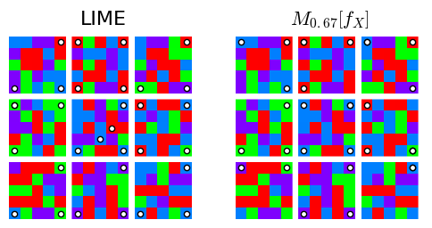
In Figure 2, we see both LIME and input gradients identify the same relevant pixels, which suggests that (1) both methods are effective at explaining model predictions, and (2) the model has learned the corner rather than the top-middle rule, which it did consistently across random restarts.

Figure 3: Implicit rule transitions as we increase $\lambda_{1}$ and the number of nonzero rows of $A$. Pairs of points represent the fraction of large-magnitude ($c=0.67$) gradient components in the corners and top-middle for 1000 test examples, which almost always add to 1 (indicating the model is most sensitive to these elements alone, even during transitions). Note there is a wide regime where the model learns a hybrid of both rules.

Figure 4: Rule discovery using find-another-explanation method with 0.67 cutoff and $\lambda_{1}=10^{3}$ for $\theta_{1}$ and $\lambda_{1}=10^{6}$ for $\theta_{2}$. Note how the first two iterations produce explanations corresponding to the two rules in the dataset while the third produces very noisy explanations (with low accuracies).

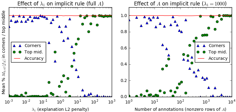
However, if we train our model with a nonzero $A$ (specifically, setting $A_{nd}=1$ for corners $d$ across examples $n$), we were able to cause it to use the other rule. Figure 3 shows how the model transitions between rules as we vary $\lambda_{1}$ and the number of examples penalized by $A$. This result demonstrates that the model can be made to learn multiple rules despite only one being commonly reached via standard gradient-based optimization methods. However, it depends on knowing a good setting for $A$, which in this case would still require annotating on the order of $10^{3}$ examples, or 5% of our dataset (although always including examples with annotations in Adam minibatches let us consistently switch rules with only 50 examples, or 0.2% of the dataset).

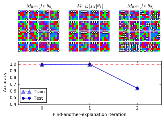
Finally, Figure 4 shows we can use the find-another-explanation technique from Sec. 2 to discover the other rule without being given $A$. Because only two rules lead to high accuracy on the test set, the model performs no better than random guessing when prevented from using either one (although we have to increase the penalty high enough that this accuracy number may be misleading - the essential point is that after the first iteration, explanations stop changing). Lastly, though not directly relevant to the discussion on interpretability and explanation, we demonstrate the potential of explanations to reduce the amount of data required for training in Appendix 1.B.

2 Real-world Datasets

To demonstrate real-world, cross-domain applicability, we test our approach on variants of three familiar machine learning text, image, and tabular datasets:

• 20 Newsgroups: As in Ribeiro et al. (2016), we test input gradients on the alt.atheism vs. soc.religion.christian subset of the 20 Newsgroups dataset Lichman (2013). We used the same two-hidden layer network architecture with a TF-IDF vectorizer with 5000 components, which gave us a 94% accurate model for $A=0$.

• Iris-Cancer: We concatenated all examples in classes 1 and 2 from the Iris dataset with the the first 50 examples from each class in the Breast Cancer Wisconsin dataset (Lichman, 2013) to create a composite dataset $X\in\mathbb{R}^{100\times 34},y\in\{0,1\}$. Despite the dataset’s small size, our network still obtains an average test accuracy of 92% across 350 random $\frac{2}{3}$-$\frac{1}{3}$ training-test splits. However, when we modify our test set to remove the 4 Iris components, average test accuracy falls to 81% with higher variance, suggesting the model learns to depend on Iris features and suffers without them. We verify that our explanations reveal this dependency and that regularizing them avoids it.

• Decoy MNIST: On the baseline MNST dataset (LeCun et al., 2010), our network obtains 98% train and 96% test accuracy. However, in Decoy MNIST, images $x$ have $4\times 4$ gray swatches in randomly chosen corners whose shades are functions of their digits $y$ in training (in particular, $255-25y$) but are random in test. On this dataset, our model has a higher 99.6% train accuracy but a much lower 55% test accuracy, indicating that the decoy rule misleads it. We verify that both gradient and LIME explanations let users detect this issue and that explanation regularization lets us overcome it.

Figure 5: Words identified by LIME vs. gradients on an example from the atheism vs. Christianity subset of 20 Newsgroups. More examples are available at https://github.com/dtak/rrr. Words are blue if they support soc.religion.christian and orange if they support alt.atheism, with opacity equal to the ratio of the magnitude of the word’s weight to the largest magnitude weight. LIME generates sparser explanations but the weights and signs of terms identified by both methods match closely. Note that both methods reveal some aspects of the model that are intuitive (“church” and “service” are associated with Christianity), some aspects that are not (“13” is associated with Christianity, “edu” with atheism), and some that are debatable (“freedom” is associated with atheism, “friends” with Christianity).

Figure 6: Input gradient explanations for Decoy MNIST vs. LIME, using the LIME image library Ribeiro (2016). In this example, the model incorrectly predicts 3 rather than 7 because of the decoy swatch.

Figure 7: Iris-Cancer features identified by input gradients vs. LIME, with Iris features highlighted in red. Input gradient explanations are more faithful to the model. Note that most gradients change sign when switching between $\hat{y}_{0}$ and $\hat{y}_{1}$, and that the magnitudes of input gradients are different across examples, which provides information about examples’ proximity to the decision boundary.

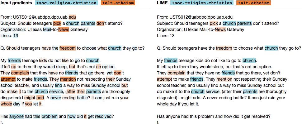
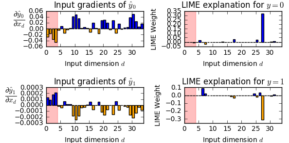
Input gradients are consistent with sample-based methods such as LIME, and faster. On 20 Newsgroups (Figure 5), input gradients are less sparse but identify all of the same words in the document with similar weights. Note that input gradients also identify words outside the document that would affect the prediction if added.

On Decoy MNIST (Figure 6), both LIME and input gradients reveal that the model predicts 3 rather than 7 due to the color swatch in the corner. Because of their fine-grained resolution, input gradients sometimes better capture counterfactual behavior, where extending or adding lines outside of the digit to either reinforce it or transform it into another digit would change the predicted probability (see also Figure 10). LIME, on the other hand, better captures the fact that the main portion of the digit is salient (because its super-pixel perturbations add and remove larger chunks of the digit).

On Iris-Cancer (Figure 7), input gradients actually outperform LIME. We know from the accuracy difference that Iris features are important to the model’s prediction, but LIME only identifies a single important feature, which is from the Breast Cancer dataset (even when we vary its perturbation strategy). This example, which is tabular and contains continuously valued rather categorical features, may represent a pathological case for LIME, which operates best when it can selectively mask a small number of meaningful chunks of its inputs to generate perturbed samples. For truly continuous inputs, it should not be surprising that explanations based on gradients perform best.

There are a few other advantages input gradients have over sample-based perturbation methods. On 20 Newsgroups, we noticed that for very long documents, explanations generated by the sample-based method LIME are often overly sparse, and there are many words identified as significant by input gradients that LIME ignores. This may be because the number of features LIME selects must be passed in as a parameter beforehand, and it may also be because LIME only samples a fixed number of times. For sufficiently long documents, it is unlikely that sample-based approaches will mask every word even once, meaning that the output becomes increasingly nondeterministic—an undesirable quality for explanations. To resolve this issue, one could increase the number of samples, but that would increase the computational cost since the model must be evalutated at least once per sample to fit a local surrogate. Input gradients, on the other hand, only require on the order of one model evaluation total to generate an explanation of similar quality (generating gradients is similar in complexity to predicting probabilities), and furthermore, this complexity is based on the vector length, not the document length. This issue (underscored by Table 1) highlights some inherent scalability advantages input gradients enjoy over sample-based perturbation methods.

	LIME	Gradients	Dimension of $x$
Iris-Cancer	0.03s	0.000019s	34
Toy Colors	1.03s	0.000013s	75
Decoy MNIST	1.54s	0.000045s	784
20 Newsgroups	2.59s	0.000520s	5000

Table 1: Gradient vs. LIME runtimes per explanation. Note that each method uses a different version of LIME; Iris-Cancer and Toy Colors use lime_tabular with continuous and quartile-discrete perturbation methods, respectively, Decoy MNIST uses lime_image, and 20 Newsgroups uses lime_text. Code was executed on a laptop and input gradient calculations were not optimized for performance, so runtimes are only meant to provide a sense of scale.

Figure 8: Overcoming confounds using explanation constraints on Iris-Cancer (over 350 random train-test splits). By default ($A=0$), input gradients tend to be large in Iris dimensions, which results in lower accuracy when Iris is removed from the test set. Models trained with $A_{nd}=1$ in Iris dimensions (full $A$) have almost exactly the same test accuracy with and without Iris.

Figure 9: Training with explanation constraints on Decoy MNIST. Accuracy is low ($A=0$) on the swatch color-randomized test set unless the model is trained with $A_{nd}=1$ in swatches (full $A$). In that case, test accuracy matches the same architecture’s performance on the standard MNIST dataset (baseline).

 
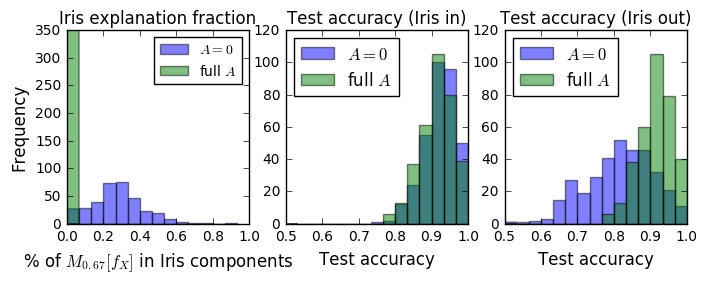
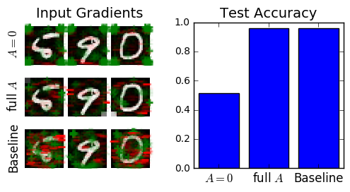
Given annotations, input gradient regularization finds solutions consistent with domain knowledge. Another key advantage of using an explanation method more closely related to our model is that we can then incorporate explanations into our training process, which are most useful when the model faces ambiguities in how to classify inputs. We deliberately constructed the Decoy MNIST and Iris-Cancer datasets to have this kind of ambiguity, where a rule that works in training will not generalize to test. When we train our network on these confounded datasets, their test accuracy is better than random guessing, in part because the decoy rules are not simple and the primary rules not complex, but their performance is still significantly worse than on a baseline test set with no decoy rules. By penalizing explanations we know to be incorrect using the loss function defined in Section 1, we are able to recover that baseline test accuracy, which we demonstrate in Figures 8 and 9.

Figure 10: Find-another-explanation results on Iris-Cancer (top; errorbars show standard deviations across 50 trials), 20 Newsgroups (middle; blue supports Christianity and orange supports atheism, word opacity set to magnitude ratio), and Decoy MNIST (bottom, for three values of $\lambda_{1}$ with scatter opacity set to magnitude ratio cubed). Real-world datasets are often highly redundant and allow for diverse models with similar accuracies. On Iris-Cancer and Decoy MNIST, both explanations and accuracy results indicate we overcome confounds after 1-2 iterations without any prior knowledge about them encoded in $A$.

 
When annotations are unavailable, our find-another-explanation method discovers diverse classifiers. As we saw with the Toy Color dataset, even if almost every row of $A$ is 0, we can still benefit from explanation regularization (meaning practitioners can gradually incorporate these penalties into their existing models without much upfront investment). However, annotation is never free, and in some cases we either do not know the right explanation or cannot easily encode it. Additionally, we may be interested in exploring the structure of our model and dataset in a less supervised fashion. On real-world datasets, which are usually overdetermined, we can use find-another-explanation to discover $\theta$s in shallower local minima that we would normally never explore. Given enough models right for different reasons, hopefully at least one is right for the right reasons.

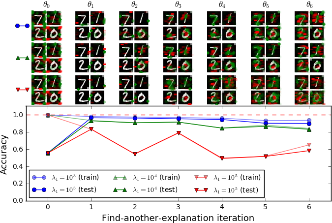
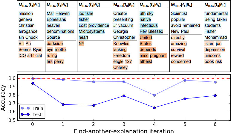
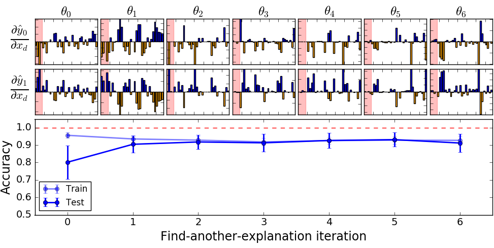
Figure 10 shows find-another-explanation results for our three real-world datasets, with example explanations at each iteration above and model train and test accuracy below. For Iris-Cancer, we find that the initial iteration of the model heavily relies on the Iris features and has high train but low test accuracy, while subsequent iterations have lower train but higher test accuracy (with smaller gradients in Iris components). In other words, we spontaneously obtain a more generalizable model without a predefined $A$ alerting us that the first four features are misleading.

Find-another-explanation also overcomes confounds on Decoy MNIST, needing only one iteration to recover baseline accuracy. Bumping $\lambda_{1}$ too high (to the point where its term is a few orders of magnitude larger than the cross-entropy) results in more erratic behavior. Interestingly, in a process remniscent of distillation (Papernot et al., 2016c), the gradients themselves become more evenly and intuitively distributed at later iterations. In many cases they indicate that the probabilities of certain digits increase when we brighten pixels along or extend their distinctive strokes, and that they decrease if we fill in unrelated dark areas, which seems desirable. However, by the last iteration, we start to revert to using decoy swatches in some cases.

On 20 Newsgroups, the words most associated with alt.atheism and
soc.religion.christian change between iterations but remain mostly intuitive in their associations. Train accuracy mostly remains high while test accuracy is unstable.

For all of these examples, accuracy remains high even as decision boundaries shift significantly. This may be because real-world data tends to contain significant redundancies.

3 Limitations

Input gradients provide faithful information about a model’s rationale for a prediction but trade interpretability for efficiency. In particular, when input features are not individually meaningful to users (e.g. for individual pixels or word2vec components), input gradients may be difficult to interpret and $A$ may be difficult to specify. Additionally, because they can be 0 far from the decision boundary, they do not capture the idea of salience as well as other methods (Zeiler and Fergus, 2014; Sundararajan et al., 2017; Montavon et al., 2017; Bach et al., 2015; Shrikumar et al., 2016). However, they are necessarily faithful to the model and easy to incorporate into its loss function. Input gradients are first-order linear approximations of the model; we might call them first-order explanations.

4 Discussion

In this chapter, we showed that:

• On training sets that contain confounds which would fool any model trained just to make correct predictions, we can use gradient-based explanation regularization to learn models that still generalize to test. These results imply that gradient regularization actually changes why our model makes predictions.

• When we lack expert annotations, we can still use our method in an unsupervised manner to discover models that make predictions for different reasons. This “find-another-explanation” technique allowed us to overcome confounds on Decoy MNIST and Iris-Cancer, and even quantify the ambiguity present in the Toy Color dataset.

• Input gradients are consistent with sample-based methods such as LIME but faster to compute and sometimes more faithful to the model, especially for continuous inputs.

Our consistent results on several diverse datasets show that input gradients merit further investigation as building blocks for optimizable explanations; there exist many options for further advancements such as weighted annotations $A$, different penalty norms, and more general specifications of whether features should be positively or negatively predictive of specific classes for specific inputs.

Finally, our “right for the right reasons” approach may be of use in solving related problems, e.g. in integrating causal inference with deep neural networks or maintaining robustness to adversarial examples (which we discuss in Chapter 2). Building on our find-another-explanation results, another promising direction is to let humans in the loop interactively guide models towards correct explanations. Overall, we feel that developing methods of ensuring that models are right for better reasons is essential to overcoming the inherent obstacles to generalization posed by ambiguities in real-world datasets.

Appendix 1.A Cross-Validation

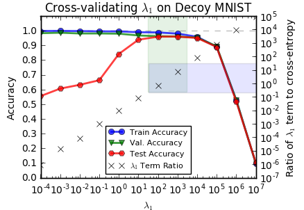
Most regularization parameters are selected to maximize accuracy on a validation set. However, when your training and validation sets share the same misleading confounds, validation accuracy may not be a good proxy for test accuracy. Instead, we recommend increasing the explanation regularization strength $\lambda_{1}$ until the cross-entropy and “right reasons” terms have roughly equal magnitudes (which corresponds to the region of highest test accuracy below). Intuitively, balancing the terms in this way should push our optimization away from cross-entropy minima that violate the explanation constraints specified in $A$ and towards ones that correspond to “better reasons.” Increasing $\lambda_{1}$ too much makes the cross-entropy term negligible. In that case, our model performs no better than random guessing.

Figure 11: Cross-validating $\lambda_{1}$. The regime of highest accuracy (highlighted) is also where the initial cross-entropy and $\lambda_{1}$ loss terms have similar magnitudes. Exact equality is not required; being an order of magnitude off does not significantly affect accuracy.

Appendix 1.B Learning with Less Data

It is natural to ask whether explanations can reduce data requirements. Here we explore that question on the Toy Color dataset using four variants of $A$ (with $\lambda_{1}$ chosen to match loss terms at each $N$).

Figure 12: Explanation regularization can reduce data requirements.

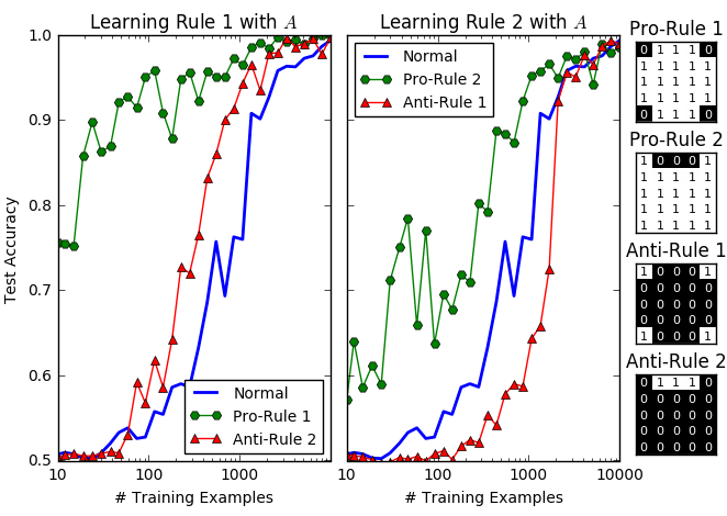
We find that when $A$ is set to the Pro-Rule 1 mask, which penalizes all pixels except the corners, we reach 95% accuracy with fewer than 100 examples (as compared to $A=0$, where we need almost 10000). Penalizing the top-middle pixels (Anti-Rule 2) or all pixels except the top-middle (Pro-Rule 2) also consistently improves accuracy relative to data. Penalizing the corners (Anti-Rule 1), however, reduces accuracy until we reach a threshold $N$. This may be because the corner pixels can match in 4 ways, while the top-middle pixels can differ in $4\cdot 3\cdot 2=24$ ways, suggesting that Rule 2 could be inherently harder to learn from data and positional explanations alone.

Appendix 1.C Simultaneous Find-Another-Explanation

In Section 2, we introduced a method of training classifiers to make predictions for different reasons by sequentially augmenting $A$ to penalize more features. However, as our ensemble grows, $A$ can saturate to $\mathbb{1}^{N\times D}$, and subsequent models will be trained with uniform gradient regularization. While these models may have desirable properties (which we explore in the following chapter), they will not be diverse.

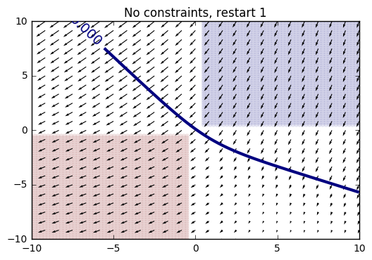
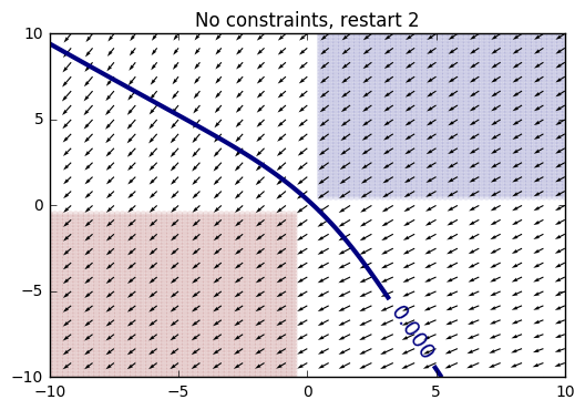
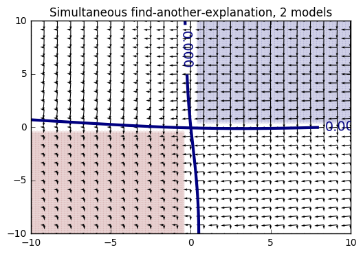
As a simple example, consider a 2D dataset with one class confined to the first quadrant and the other confined to the third. In theory, we have a full degree of decision freedom; it should be possible to learn two perfect and fully orthogonal boundaries (one horizontal, one vertical). However, when we train our first MLP, it learns a diagonal surface; both features have large gradients everywhere, so $A=\mathbb{1}^{N\times 2}$ immediately. To resolve this, we propose a simultaneous training procedure:

$$\theta_{1}^{*},\ldots,\theta_{M}^{*}=\operatorname*{arg\,min}_{\theta_{1},\ldots,\theta_{M}}\sum_{a=1}^{M}\mathcal{L}(y,f(X|\theta_{a}))+\sum_{a=1}^{M}\sum_{b=a+1}^{M}\text{{sim}}(f_{X}(X|\theta_{a}),f_{X}(X|\theta_{b})),$$ (1)

where $\mathcal{L}$ refers to our single-model loss function, and for our similarity measure we use the squared cosine similarity $\text{{sim}}(v,w)=\frac{(v^{T}w)^{2}}{(v^{T}v)(w^{T}w)+\epsilon}$, where we add $\epsilon=10^{-6}$ to the denominator for numerical stability. Squaring the cosine similarity ensures our penalty is positive, is minimized by orthogonal boundaries, and is soft for nearly orthogonal boundaries. We show in Figure 13 that this lets us obtain the two desired models.

Figure 13: Toy 2D problem with one degree of decision boundary freedom. Across random restarts (left two plots), we tend to learn a boundary in which both features are significant, which prevents sequential find-another-explanation from producing diverse models. If we jointly train two models with a penalty on the cosine similarity of their gradients (right plot), they end up with orthogonal boundaries.

Chapter 2 Interpretability and Robustness

1 Introduction

In the previous chapter, we used input gradient penalties to encourage neural networks to make predictions for specific reasons. We demonstrated this on “decoy” datasets deliberately designed to deceive models making decisions for different reasons. This philosophy of testing – that we should measure generalization by testing on data from a different distribution than we trained on – can be taken to its extreme by testing models in an adversarial setting, where neural networks have known vulnerabilities (Szegedy et al., 2013). In this chapter, we consider whether a domain knowledge-agnostic application of explanation regularization (a uniform L2 penalty on input gradients, similar in spirit to Ridge regression on the model’s local linear approximations) could help defend against adversarial examples.

Adversarial examples pose serious obstacles for the adoption of neural networks in settings which are security-sensitive or have legal ramifications (Kang and Kang, 2017). Although many techniques for generating these examples (which we call “attacks”) require access to model parameters, Papernot et al. (2017) have shown that it is possible and even practical to attack black-box models in the real world, in large part because of transferability; examples generated to fool one model tend to fool all models trained on the same dataset. Particularly for images, these adversarial examples can be constructed to fool models across a variety of scales and perspectives (Athalye and Sutskever, 2017), which poses a problem for the adoption of deep learning models in systems like self-driving cars.

Although there has recently been a great deal of research in adversarial defenses, many of these methods have struggled to achieve robustness to transferred adversarial examples (Tramèr et al., 2017b). Some of the most effective defenses simply detect and reject them rather than making predictions (Xu et al., 2017). The most common, “brute force” solution is adversarial training, where we include a mixture of normal and adversarially-generated examples in the training set (Kurakin et al., 2016b). However, Tramèr et al. (2017a) show that the robustness adversarial training provides can be circumvented by randomizing or transferring perturbations from other models (though ensembling helps).

As we noted in Chapter 1, domain experts are also often concerned that DNN predictions are uninterpretable. The lack of interpretability is particularly problematic in domains where algorithmic bias is often a factor (Angwin et al., 2016) or in medical contexts where safety risks can arise when there is mismatch between how a model is trained and used (Caruana et al., 2015). For computer vision models (the primary target of adversarial attacks), the most common class of explanation is the saliency map, either at the level of raw pixels, grid chunks, or superpixels (Ribeiro et al., 2016).

The local linear approximation provided by raw input gradients (Baehrens et al., 2010) is sometimes used for pixel-level saliency maps (Simonyan et al., 2013). However, computer vision practitioners tend not to examine raw input gradients because they are noisy and difficult to interpret. This issue has spurred the development of techniques like integrated gradients (Sundararajan et al., 2017) and SmoothGrad (Smilkov et al., 2017) that generate smoother, more interpretable saliency maps from noisy gradients. The rationale behind these techniques is that, while the local behavior of the model may be noisy, examining the gradients over larger length scales in input space provides a better intution about the model’s behavior.

However, raw input gradients are exactly what many attacks use to generate adversarial examples. Explanation techniques which smooth out gradients in background pixels may be inappropriately hiding the fact that the model is quite sensitive to them. We consider that perhaps the need for these smoothing techniques in the first place is indicative of a problem with our models, related to their adversarial vulnerability and capacity to overfit. Perhaps it is fundamentally hard for adversarially vulnerable models to be interpretable.

On the other hand, perhaps it is hard for interpretable models to be adversarially vulnerable. Our hypothesis is that by training a model to have smooth input gradients with fewer extreme values, it will not only be more interpretable but also more resistant to adversarial examples. In the experiments that follow we confirm this hypothesis using uniform gradient regularization, which optimizes the model to have smooth input gradients with respect to its predictions during training. Using this technique, we demonstrate robustness to adversarial examples across multiple model architectures and datasets, and in particular demonstrate robustness to transferred adversarial examples: gradient-regularized models maintain significantly higher accuracy on examples generated to fool other models than baselines. Furthermore, both qualitatively and in human subject experiments, we find that adversarial examples generated to fool gradient-regularized models are, in a particular sense, more “interpretable”: they fool humans as well.

2 Background

In this section, we will (re)introduce notation, and give a brief overview of the baseline attacks and defenses against which we will test and compare our methods. The methods we will analyze again apply to all differentiable classification models $f_{\theta}(X)$, which are functions parameterized by $\theta$ that return predictions $\hat{y}\in\mathbb{R}^{N\times K}$ given inputs $X\in\mathbb{R}^{N\times D}$. These predictions indicate the probabilities that each of $N$ inputs in $D$ dimensions belong to each of $K$ class labels. To train these models, we try to find sets of parameters $\theta^{*}$ that minimize the total information distance between the predictions $\hat{y}$ and the true labels $y$ (also $\in\mathbb{R}^{N\times K}$, one-hot encoded) on a training set:

$$\begin{split}\theta^{*}&=\operatorname*{arg\,min}_{\theta}\sum_{n=1}^{N}\sum_{k=1}^{K}-y_{nk}\log f_{\theta}(X_{n})_{k},\\ \end{split}$$ (1)

which we will sometimes write as

$$\operatorname*{arg\,min}_{\theta}H(y,\hat{y}),$$

with $H$ giving the sum of the cross entropies between the predictions and the labels.

1 Attacks

Fast Gradient Sign Method (FGSM)

Goodfellow et al. (2014) introduced this first method of generating adversarial examples by perturbing inputs in a manner that increases the local linear approximation of the loss function:

$$X_{\text{FGSM}}=X+\epsilon\,\text{sign}\left(\nabla_{x}H(y,\hat{y})\right)$$ (2)

If $\epsilon$ is small, these adversarial examples are indistinguishable from normal examples to a human, but the network performs significantly worse on them.

Kurakin et al. (2016a) noted that one can iteratively perform this attack with a small $\epsilon$ to induce misclassifications with a smaller total perturbation (by following the nonlinear loss function in a series of small linear steps rather than one large linear step).

Targeted Gradient Sign Method (TGSM)

A simple modification of the Fast Gradient Sign Method is the Targeted Gradient Sign Method, introduced by Kurakin et al. (2016a). In this attack, we attempt to decrease a modified version of the loss function that encourages the model to misclassify examples in a specific way:

$$X_{\text{TGSM}}=X-\epsilon\,\text{sign}\left(\nabla_{x}H(y_{\text{target}},\hat{y})\right),$$ (3)

where $y_{\text{target}}$ encodes an alternate set of labels we would like the model to predict instead. In the digit classification experiments below, we often picked targets by incrementing the labels $y$ by 1 (modulo 10), which we will refer to as $y_{+1}$. The TGSM can also be performed iteratively.

Jacobian-based Saliency Map Approach (JSMA)

The final attack we consider, the Jacobian-based Saliency Map Approach (JSMA), also takes an adversarial target vector $y_{\text{target}}$. It iteratively searches for pixels or pairs of pixels in $X$ to change such that the probability of the target label is increased and the probability of all other labels are decreased. This method is notable for producing examples that have only been changed in several dimensions, which can be hard for humans to detect. For a full description of the attack, we refer the reader to Papernot et al. (2016b).

2 Defenses

As baseline defenses, we consider defensive distillation and adversarial training. To simplify comparison, we omit defenses (Xu et al., 2017; Nayebi and Ganguli, 2017) that are not fully architecture-agnostic or which work by detecting and rejecting adversarial examples.

Distillation

Distillation, originally introduced by Ba and Caruana (2014), was first examined as a potential defense by Papernot et al. (2016c). The main idea is that we train the model twice, initially using the one-hot ground truth labels but ultimately using the initial model’s softmax probability outputs, which contain additional information about the problem. Since the normal softmax function tends to converge very quickly to one-hot-ness, we divide all of the logit network outputs (which we will call $\hat{z}_{k}$ instead of the probabilities $\hat{y}_{k}$) by a temperature $T$ (during training but not evaluation):

$$f_{T,\theta}(X_{n})_{k}=\frac{e^{\hat{z}_{k}(X_{n})/T}}{\sum_{i=1}^{K}e^{\hat{z}_{i}(X_{n})/T}},$$ (4)

where we use $f_{T,\theta}$ to denote a network ending in a softmax with temperature $T$. Note that as $T$ approaches $\infty$, the predictions converge to $\frac{1}{K}$. The full process can be expressed as

$$\begin{split}\theta^{0}&=\operatorname*{arg\,min}_{\theta}\sum_{n=1}^{N}\sum_{k=1}^{K}-y_{nk}\log f_{T,\theta}(X_{n})_{k},\\ \theta^{*}&=\operatorname*{arg\,min}_{\theta}\sum_{n=1}^{N}\sum_{k=1}^{K}-f_{T,\theta^{0}}(X_{n})_{k}\log f_{T,\theta}(X_{n})_{k}.\end{split}$$ (5)

Distillation is usually used to help small networks achieve the same accuracy as larger DNNs, but in a defensive context, we use the same model twice. It has been shown to be an effective defense against white-box FGSM attacks, but Carlini and Wagner (2016) have shown that it is not robust to all kinds of attacks. We will see that the precise way it defends against certain attacks is qualitatively different than gradient regularization, and that it can actually make the models more vulnerable to attacks than an undefended model.

Adversarial Training

In adversarial training (Kurakin et al., 2016b), we increase robustness by injecting adversarial examples into the training procedure. We follow the method implemented in Papernot et al. (2016a), where we augment the network to run the FGSM on the training batches and compute the model’s loss function as the average of its loss on normal and adversarial examples without allowing gradients to propogate so as to weaken the FGSM attack (which would also make the method second-order). We compute FGSM perturbations with respect to predicted rather than true labels to prevent “label leaking,” where our model learns to classify adversarial examples more accurately than regular examples.

3 Gradient Regularization

We defined our “right for the right reasons” objective in Chapter 1 using an L2 penalty on the gradient of the model’s predictions across classes with respect to input features marked irrelevant by domain experts. We encoded their domain knowledge using an annotation matrix $A$. If we set $A=1$, however, and consider only the log-probabilities of the predicted classes, we recover what Drucker and Le Cun (1992) introduced as “double backpropagation”, which trains neural networks by minimizing not just the “energy” of the network but the rate of change of that energy with respect to the input features. In their formulation the energy is a quadratic loss, but we can reformulate it almost equivalently using the cross-entropy:

$$\theta^{*}=\operatorname*{arg\,min}_{\theta}\sum_{n=1}^{N}\sum_{k=1}^{K}-y_{nk}\log f_{\theta}(X_{n})_{k}+\lambda\sum_{d=1}^{D}\sum_{n=1}^{N}\left(\frac{\partial}{\partial x_{d}}\sum_{k=1}^{K}-y_{nk}\log f_{\theta}(X_{n})_{k}\right)^{2},$$ (6)

whose objective we can write a bit more concisely as

$$\operatorname*{arg\,min}_{\theta}H(y,\hat{y})+\lambda||\nabla_{x}H(y,\hat{y})||_{2}^{2},$$

where $\lambda$ is again a hyperparameter specifying the penalty strength. The intuitive objective of this function is to ensure that if any input changes slightly, the divergence between the predictions and the labels will not change significantly (though including this term does not guarantee Lipschitz continuity everywhere). Double backpropagation was mentioned as a potential adversarial defense in the same paper which introduced defensive distillation (Papernot et al., 2016c), but at publish time, its effectiveness in this respect had not yet been analyzed in the literature – though Gu and Rigazio (2014) previously and Hein and Andriushchenko (2017); Czarnecki et al. (2017) concurrently consider related objectives, and Raghunathan et al. (2018) derive and minimze an upper bound on adversarial vulnerability based on the maximum gradient norm in a ball around each training input. These works also provide stronger theoretical explanations for why input gradient regularization is effective, though they do not analyze its relationship to model interpretability. In this work, we interpret gradient regularization as a quadratic penalty on our model’s saliency map.

4 Experiments

Datasets and Models

We evaluated the robustness of distillation, adversarial training, and gradient regularization to the FGSM, TGSM, and JSMA on MNIST (LeCun et al., 2010), Street-View House Numbers (SVHN) (Netzer et al., 2011), and notMNIST Butalov (2011). On all datasets, we test a simple convolutional neural network with 5x5x32 and 5x5x64 convolutional layers followed by 2x2 max pooling and a 1024-unit fully connected layer, with batch-normalization after all convolutions and both batch-normalization and dropout on the fully-connected layer. All models were implemented in Tensorflow and trained using Adam (Kingma and Ba, 2014) with $\alpha=0.0002$ and $\epsilon=10^{-4}$ for 15000 minibatches of size of 256. For SVHN, we prepare training and validation set as described in Sermanet et al. (2012), converting the images to grayscale following Grundland and Dodgson (2007) and applying both global and local contrast normalization.

Attacks and Defenses

Figure 1: Accuracy of all CNNs on FGSM examples generated to fool undefended models, defensively distilled, adversarially trained, and gradient regularized models (from left to right) on MNIST, SVHN, and notMNIST (from top to bottom). Gradient-regularized models are the most resistant to other models’ adversarial examples at high $\epsilon$, while all models are fooled by gradient-regularized model examples. On MNIST and notMNIST, distilled model examples are usually identical to non-adversarial examples (due to gradient underflow), so they fail to fool any of the other models.

Figure 2: Applying both gradient regularization and adversarial training (“both defenses”) allows us to obtain maximal robustness to white-box and normal black-box attacks on SVHN (with a very slight label-leaking effect on the FGSM, perhaps due to the inclusion of the $\nabla_{x}H(y,\hat{y})$ term). However, no models are able to maintain robustness to black-box attacks using gradient regularization.

For adversarial training and JSMA example generation, we used the Cleverhans adversarial example library (Papernot et al., 2016a). For distillation, we used a softmax temperature of $T=50$, and for adversarial training, we trained with FGSM perturbations at $\epsilon=0.3$, averaging normal and adversarial losses. For gradient regularized models, we use double backpropagation, which provided the best robustness, and train over a spread of $\lambda$ values. We choose the $\lambda$ with the highest accuracy against validation black-box FGSM examples but which is still at least 97% as accurate on normal validation examples (though accuracy on normal examples tended not to be significantly different). Code for all models and experiments has been open-sourced.

Evaluation Metrics

For the FGSM and TGSM, we test all models against adversarial examples generated for each model and report accuracy. Testing this way allows us to simultaneously measure white- and black-box robustness.

On the JSMA and iterated TGSM, we found that measuring accuracy was no longer a good evaluation metric, since for our gradient-regularized models, the generated adversarial examples often resembled their targets more than their original labels. To investigate this, we performed a human subject experiment to evaluate the legitimacy of adversarial example misclassifications.

1 Accuracy Evaluations (FGSM and TGSM)

FGSM Robustness

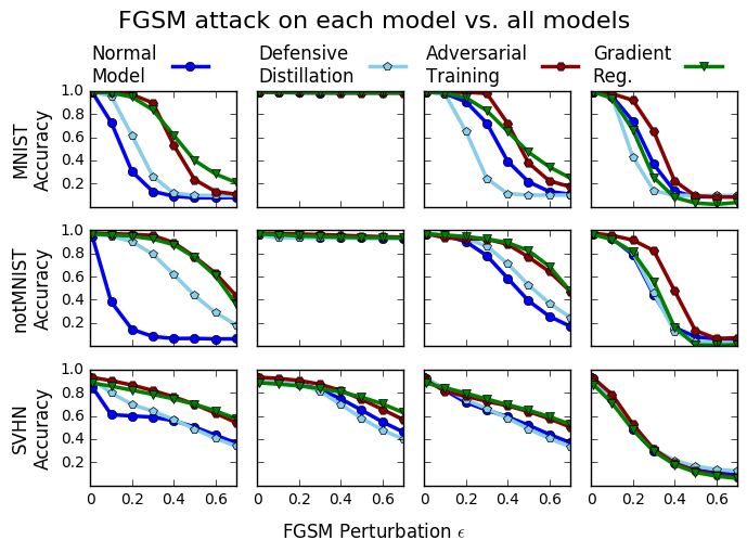
Figure 1 shows the results of our defenses’ robustness to the FGSM on MNIST, SVHN, and notMNIST for our CNN at a variety of perturbation strengths $\epsilon$. Consistently across datasets, we find that gradient-regularized models exhibit strong robustness to black-box transferred FGSM attacks (examples produced by attacking other models). Although adversarial training sometimes performs slightly better at $\epsilon\leq 0.3$, the value we used in training, gradient regularization generally surpasses it at higher $\epsilon$ (see the green curves in the leftmost plots).

The story with white-box attacks is more interesting. Gradient-regularized models are generally more robust to than undefended models (visually, the green curves in the rightmost plots fall more slowly than the blue curves in the leftmost plots). However, accuracy still eventually falls for them, and it does so faster than for adversarial training. Even though their robustness to white-box attacks seems lower, though, the examples produced by those white-box attacks actually fool all other models equally well. This effect is particularly pronounced on SVHN. In this respect, gradient regularization may hold promise not just as a defense but as an attack, if examples generated to fool them are inherently more transferable.

Models trained with defensive distillation in general perform no better and often worse than undefended models. Remarkably, except on SVHN, attacks against distilled models actually fail to fool all models. Closer inspection of distilled model gradients and examples themselves reveals that this occurs because distilled FGSM gradients vanish – so the examples are not perturbed at all. As soon as we obtain a nonzero perturbation from a different model, distillation’s appearance of robustness vanishes as well.

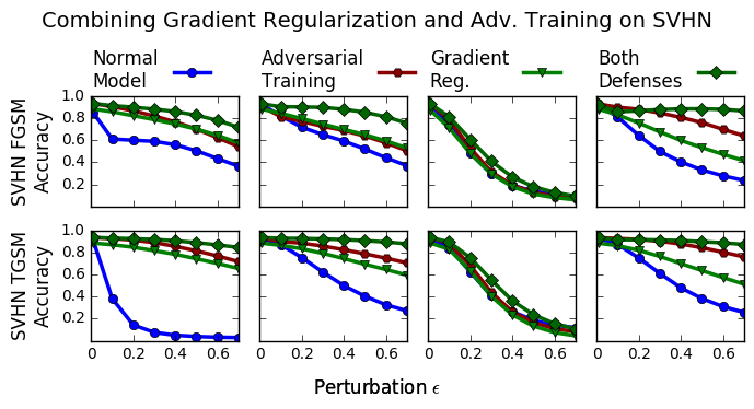
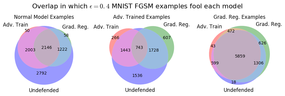
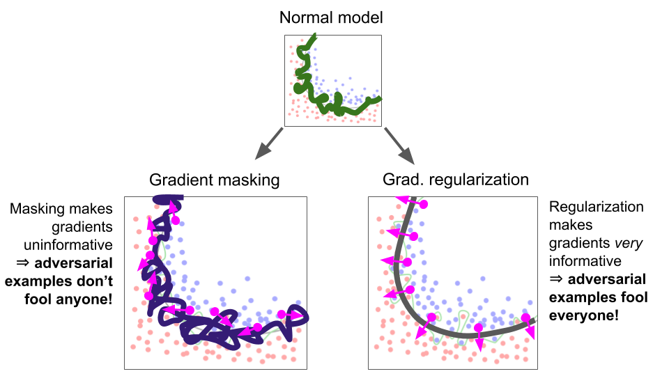
Although adversarial training and gradient regularization seem comparable in terms of accuracy, they work for different reasons and can be applied in concert to increase robustness, which we show in Figure 2. In Figure 3 we also show that, on normal and adversarially trained black-box FGSM attacks, models trained with these two defenses are fooled by different sets of adversarial examples. We provide intuition for why this might be the case in Figure 4.

Figure 3: Venn diagrams showing overlap in which MNIST $\epsilon=0.4$ FGSM examples, generated for normal, adversarially trained, and gradient regularized models, fool all three. Undefended models tend to be fooled by examples from all models, while the sets of adversarially trained model FGSM examples that fool the two defended models are closer to disjoint. Gradient-regularized model FGSM examples fool all models. These results suggest that ensembling different forms of defense may be effective in defending against black box attacks (unless those black box attacks use a gradient-regularized proxy).

Figure 4: Conceptual illustration of the difference between gradient regularization and gradient masking. In (idealized) gradient masking, input gradients are completely uninformative, so following them doesn’t affect either the masked model’s predictions or those of any other model. In gradient regularization, gradients actually become more informative, so following them will ultimately fool all models. However, because gradients are also smaller, perturbations need to be larger to flip predictions. Unregularized, unmasked models are somewhere in between. We see quantitative support for this interpretation in Figure 3, as well as qualitative evidence in Figure 9.

Figure 5: CNN accuracy on $y_{+1}$ TGSM examples generated to fool the four models on three datasets (see Figure 1 for more explanation). Gradient-regularized models again exhibit robustness to other models’ adversarial examples. Distilled model adversarial perturbations fool other models again since their input gradients no longer underflow.

TGSM Robustness

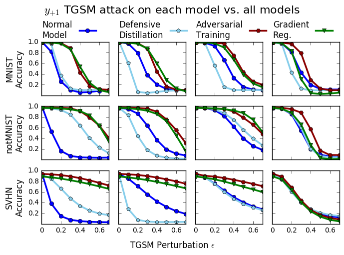
Against the TGSM attack (Figure 5), defensively distilled model gradients no longer vanish, and accordingly these models start to show the same vulnerability to adversarial attacks as others. Gradient-regularized models still exhibit the same robustness even at large perturbations $\epsilon$, and again, examples generated to fool them fool other models equally well.

Figure 6: Distributions of (L2 norm) magnitudes of FGSM input gradients (top), TGSM input gradients (middle), and predicted log probabilities across all classes (bottom) for each defense. Note the logarithmic scales. Gradient-regularized models tend to assign non-predicted classes higher probabilities, and the L2 norms of the input gradients of their FGSM and TGSM loss function terms have similar orders of magnitude. Distilled models (evaluated at $T=0$) assign extremely small probabilities to all but the predicted class, and their TGSM gradients explode while their FGSM gradients vanish (we set a minimum value of $10^{-20}$ to prevent underflow). Normal and adversarially trained models lie somewhere in the middle.

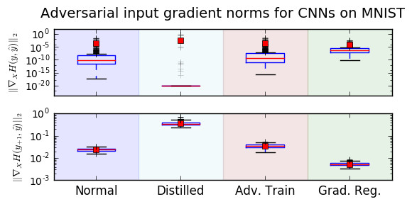
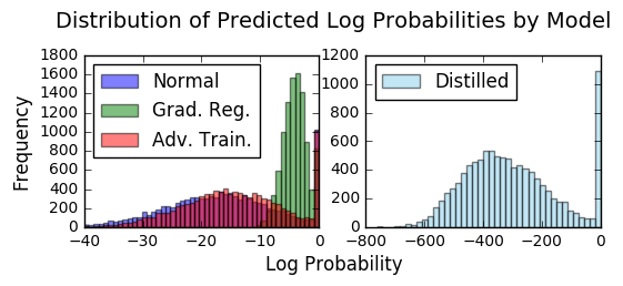
One way to better understand the differences between gradient-regularized, normal, and distilled models is to examine the log probabilities they output and the norms of their loss function input gradients, whose distributions we show in Figure 6 for MNIST. We can see that the different defenses have very different statistics. Probabilities of non-predicted classes tend to be small but remain nonzero for gradient-regularized models, while they vanish on defensively distilled models evaluated at $T=0$ (despite distillation’s stated purpose of discouraging certainty). Perhaps because $\nabla\log p(x)=\frac{1}{p(x)}\nabla p(x)$, defensively distilled models’ non-predicted log probability input gradients are the largest by many orders of magnitude, while gradient-regularized models’ remain controlled, with much smaller means and variances. The other models lie between these two extremes. While we do not have a strong theoretical argument about what input gradient magnitudes should be, we believe it makes intuitive sense that having less variable, well-behaved, and non-vanishing input gradients should be associated with robustness to attacks that consist of small perturbations in input space.

Figure 7: Results of applying the JSMA to MNIST 0 and 1 images with maximum distortion parameter $\gamma=0.25$ for a distilled model (left) and a gradient-regularized model (right). Examples in each row start out as the highlighted digit but are modified until the model predicts the digit corresponding to their column or the maximum distortion is reached.

2 Human Subject Study (JSMA and Iterated TGSM)

Need for a Study

Accuracy scores against the JSMA can be misleading, since without a maximum distortion constraint it necessarily runs until the model predicts the target. Even with such a constraint, the perturbations it creates sometimes alter the examples so much that they no longer resemble their original labels, and in some cases bear a greater resemblance to their targets. Figure 7 shows JSMA examples on MNIST for gradient-regularized and distilled models which attempt to convert 0s and 1s into every other digit. Although all of the perturbations “succeed” in changing the model’s prediction, in the gradient-regularized case, many of the JSMA examples strongly resemble their targets.

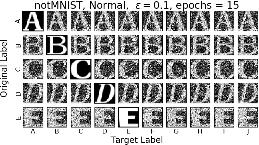
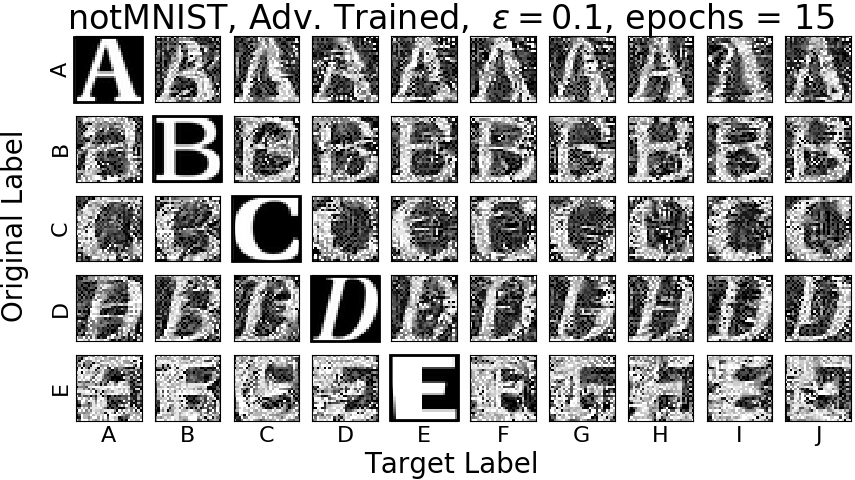
The same issues occur for other attack methods, particularly the iterated TGSM, for which we show confusion matrices for different models and datasets in Figure 8. For the gradient-regularized models, these psuedo-adversarial examples quickly become almost prototypical examples of their targets, which is not reflected in accuracies with respect to the original labels.

Figure 8: Partial confusion matrices showing results of applying the iterated TGSM for 15 iterations at $\epsilon=0.1$. Each row is generated from the same example but modified to make the model to predict every other class. TGSM examples generated for gradient-regularized models (right) resemble their targets more than their original labels and may provide insight into what the model has learned. Animated versions of these examples can be seen at http://goo.gl/q8ZM1T.

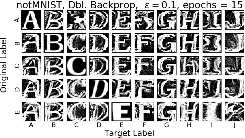
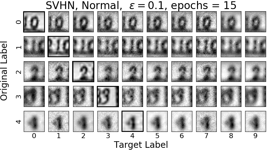
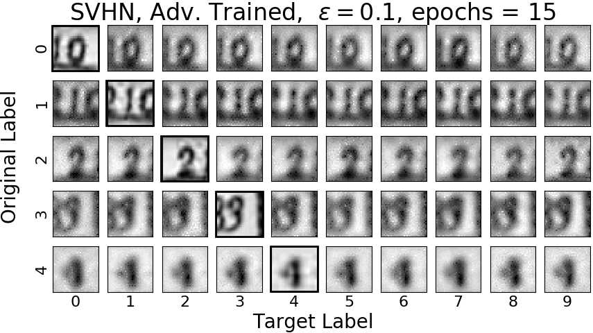
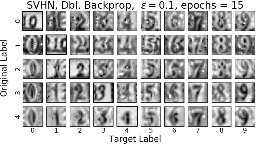
To test these intuitions more rigorously, we ran a small pilot study with 11 subjects to measure whether they found examples generated by these methods to be more or less plausible instances of their targets.

Study Protocol

The pilot study consisted of a quantitative and qualitative portion. In the quantitative portion, subjects were shown 30 images of MNIST JSMA or SVHN iterated TGSM examples. Each of the 30 images corresponded to one original digit (from 0 to 9) and one model (distilled, gradient-regularized, or undefended). Note that for this experiment, we used $\nabla_{x}H(\frac{1}{K},\hat{y})$ gradient regularization, ran the TGSM for just 10 steps, and trained models for 4 epochs at a learning rate of 0.001. This procedure was sufficient to produce examples with explanations similar to the longer training procedure used in our earlier experiments, and actually increased the robustness of the undefended models (adversarial accuracy tends to fall with training iteration). Images were chosen uniformly at random from a larger set of 45 examples that corresponded to the first 5 images of the original digit in the test set transformed using the JSMA or iterated TGSM to each of the other 9 digits (we ensured that all models misclassified all examples as their target). Subjects were not given the original label, but were asked to input what they considered the most and second-most plausible predictions for the image that they thought a reasonable classifier would make (entering N/A if they thought no label was a plausible choice). In the qualitative portion that came afterwards, users were shown three 10x10 confusion matrices for the different defenses on MNIST (Figure 7 shows the first two rows) and were asked to write comments about the differences between the examples. Afterwards, there was a short group discussion. This study was performed in compliance with the institution’s IRB.

	MNIST (JSMA)		SVHN (TGSM)
Model	human fooled	mistake reasonable	human fooled	mistake reasonable
normal	2.0%	26.0%	40.0%	63.3%
distilled	0.0%	23.5%	1.7%	25.4%
grad. reg.	16.4%	41.8%	46.3%	81.5%

Table 1: Quantitative feedback from the human subject experiment. “human fooled” columns record what percentage of examples were classified by humans as most plausibly their adversarial targets, and “mistake reasonable” records how often humans either rated the target plausible or marked the image unrecognizable as any label (N/A).

Study Results

Table 1 shows quantitative results from the human subject experiment. Overall, subjects found gradient-regularized model adversarial examples most convincing. On SVHN and especially MNIST, humans were most likely to think that gradient-regularized (rather than distilled or normal) adversarial examples were best classified as their target rather than their original digit. Additionally, when they did not consider the target the most plausible label, they were most likely to consider gradient-regularized model mispredictions “reasonable” (which we define in Table 1), and more likely to consider distilled model mispredictions unreasonable. p-values for the differences between normal and gradient regularized unreasonable error rates were 0.07 for MNIST and 0.08 for SVHN.

In the qualitative portion of the study (comparing MNIST JSMA examples), all of the written responses described significant differences between the insensitive model’s JSMA examples and those of the other two methods. Many of the examples for the gradient-regularized model were described as “actually fairly convincing,” and that the normal and distilled models “seem to be most easily fooled by adding spurious noise.” Few commentators indicated any differences between the normal and distilled examples, with several saying that “there doesn’t seem to be [a] stark difference” or that they “couldn’t describe the difference” between them. In the group discussion one subject remarked on how the perturbations to the gradient-regularized model felt “more intentional”, and others commented on how certain transitions between digits led to very plausible fakes while others seemed inherently harder. Although the study was small, both its quantitative and qualitative results support the claim that gradient regularization, at least for the two CNNs on MNIST and SVHN, is a credible defense against the JSMA and the iterated TGSM, and that distillation is not.

3 Connections to Interpretability

Figure 9: Input gradients $\nabla_{x}H(\frac{1}{K},\hat{y})$ that provide a local linear approximation of normal models (top), distilled models at $T=50$ (second from top), adversarially trained models (middle), and models trained with $\nabla_{x}H(\frac{1}{K},\hat{y})$ and $\nabla_{x}H(y,\hat{y})$ gradient regularization (bottom two). Whitening black pixels or darkening white pixels makes the model more certain of its prediction. In general, regularized model gradients appear smoother and make more intuitive sense as local linear approximations.

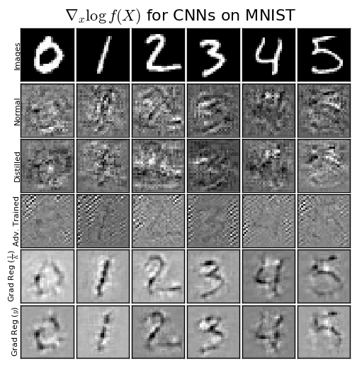
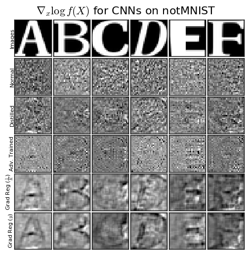
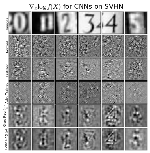
Finally, we present a qualitative evaluation suggesting a connection between adversarial robustness and interpretability. In the literature on explanations, input gradients are frequently used as explanations (Baehrens et al., 2010), but sometimes they are noisy and not interpretable on their own. In those cases, smoothing techniques have been developed (Smilkov et al., 2017; Shrikumar et al., 2016; Sundararajan et al., 2017) to generate more interpretable explanations, but we have already argued that these techniques may obscure information about the model’s sensitivity to background features.

We hypothesized that if the models had more interpretable input gradients without the need for smoothing, then perhaps their adversarial examples, which are generated directly from their input gradients, would be more interpretable as well. That is, the adversarial example would be more obviously transformative away from the original class label and towards another. The results of the user study show that our gradient-regularized models have this property; here we ask if the gradients are more interpretable as explanations.

In Figure 9 we visualize input gradients across models and datasets, and while we cannot make any quantitative claims, there does appear to be a qualitative difference in the interpretability of the input gradients between the gradient-regularized models (which were relatively robust to adversarial examples) and the normal and distilled models (which were vulnerable to them). Adversarially trained models seem to exhibit slightly more interpretable gradients, but not nearly to the same degree as gradient-regularized models. When we repeatedly apply input gradient-based perturbations using the iterated TGSM (Figure 8), this difference in interpretability between models is greatly magnified, and the results for gradient-regularized models seem to provide insight into what the model has learned. When gradients become interpretable, adversarial images start resembling feature visualizations Olah et al. (2017); in other words, they become explanations.

5 Discussion

In this chapter, we showed that:

• Gradient regularization slightly outperforms adversarial training (the SOTA) as a defense against black-box transferred FGSM examples from undefended models.

• Gradient regularization significantly increases robustness to white-box attacks, though not quite as much as adversarial training.

• Adversarial examples generated to fool gradient-regularized models are more “universal;” they are more effective at fooling all models than examples from unregularized models.

• Adversarial examples generated to fool gradient-regularized models are more interpretable to humans, and examples generated from iterative attacks quickly come to legitimately resemble their targets. This is not true for distillation or adversarial training.

The conclusion that we would like to reach is that gradient-regularized models are right for better reasons. Although they are not completely robust to attacks, their correct predictions and their mistakes are both easier to understand. To fully test this assertion, we would need to run a larger and more rigorous human subject evaluation that also tests adversarial training and other attacks beyond the JSMA, FGSM, and TGSM.

Connecting what we have done back to the general idea of explanation regularization, we saw in Equation 6 that we could interpret our defense as a quadratic penalty on our CNN’s saliency map. Imposing this penalty had both quantitative and qualitative effects; our gradients became smaller but also smoother with fewer high-frequency artifacts. Since gradient saliency maps are just normals to the model’s decision surface, these changes suggest a qualitative difference in the “reasons” behind our model’s predictions. Many techniques for generating smooth, simple saliency maps for CNNs not based on raw gradients have been shown to vary under meaningless transformations of the model Kindermans et al. (2017) or, more damningly, to remain invariant under extremely meaningful ones (Adebayo et al., 2018) – which suggests that many of these methods either oversimplify or aren’t faithful to the models they are explaining. Our approach in this chapter was, rather than simplifying our explanations of fixed models, to optimize our models to have simpler explanations. Their increased robustness can be thought of as a useful side effect.

Although the problem of adversarial robustness in deep neural networks is still very much an open one, these results may suggest a deeper connection between it and interpretability. No matter what method proves most effective in the general case, we suspect that any progress towards ensuring either interpretability or adversarial robustness in deep neural networks will likely represent progress towards both.

Chapter 3 General Explanation Regularization

In the previous two chapters, we introduced the idea of explanation regularization, and showed that we could use this to obtain models that were both simpler and more robust to differences between training and test conditions. However, we obtained all of those results just with L2 input gradient penalties. Although gradients have special importance in differentiable models such as neural networks, they have major limitations, especially when the kind of constraints we would like to impose on an explanation are abstract in a way we cannot easily relate back to input features. So in this chapter, we outline promising avenues towards more general forms of explanation regularization.

1 Alternative Input Gradient Penalties

Before we leave input gradients behind altogether, it is worth considering what else we can do with them besides simple L2 regularization.

1 L1 Regularization

In Chapter 2, we saw that penalizing the L2 norm of our model’s input gradients encouraged gradient interpretability and prediction robustness to adversarial examples, and drew an analogy to Ridge regression. One natural question to ask is how penalizing the L1 norm instead would compare, which we could understand as a form of local linear LASSO.

For a discussion of this question with application to sepsis treatment, we refer the reader to Ross et al. (2017a), which includes a case-study showing how L1 gradient regularization can help us obtain mortality risk models that are locally sparse and more consistent with clinical knowledge.

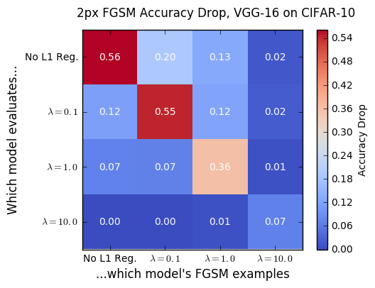
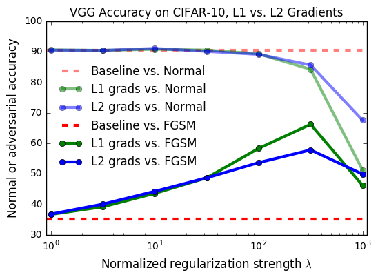
On image datasets (where input features are not individually meaningful), we do find that L1 gradient regularization is effective in defending against adversarial examples, perhaps more so than L2 regularization. To that end, in Figure 1 we present results for VGG-16 models on CIFAR-10, which bode favorably for L1 regularization against both white- and black-box attacks. However, although the gradients of these models change qualitatively compared to normal models, they are not significantly sparser than gradients of models trained with L2 gradient regularization. These results suggest that sparsity with respect to input features may not be a fully achievable or desirable objective for complex image classification tasks.

Figure 1: Left: Accuracy loss on CIFAR-10 FGSM examples ($\epsilon=2$px) for VGG models trained with varying levels of L1 gradient regularization. Diagonals measure white-box vulnerability and off-diagonals measure transferability. Right: L1 vs. L2 gradient regularization on VGG as a defense against white-box FGSM examples, 2px perturbation. The value of $\lambda$ is multiplied by 100 for the L1 regularized network to equalize penalty magnitudes (since we do not take the square root of the L2 penalty). Compared to L2, L1 gradient regularized models tend to be more robust to $l_{\infty}$ attacks like the FGSM, and their adversarial examples tend to be less transferable.

2 Higher-Order Derivatives

Bishop (1993) introduced the idea of limiting the curvature of the function learned by a neural network by imposing an L2 penalty on the network’s second input derivatives. They note, however, that evaluating these second derivatives increases the computational complexity of training by a factor of $D$, the number of input dimensions. This scaling behavior poses major practical problems for datasets like ImageNet, whose inputs are over 150,000-dimensional. Rifai et al. (2011) develop a scalable workaround by estimating the Frobenius norm of the input Hessian as $\frac{1}{\sigma^{2}}\mathbb{E}\left[\left|\left|\nabla_{X}f(x)-\nabla_{X}f(x+\epsilon)\right|\right|^{2}_{2}\right]$ for $\epsilon\stackrel{{\scriptstyle iid}}{{\sim}}\mathcal{N}(0,\sigma^{2})$, which converges to the true value as $\sigma\to 0$. They then train autoencoders whose exact gradient and approximate Hessian norms are both L2-penalized, and find that the unsupervised representations they learn are more useful for downstream classification tasks. Czarnecki et al. (2017) also regularize using estimates of higher-order derivatives.

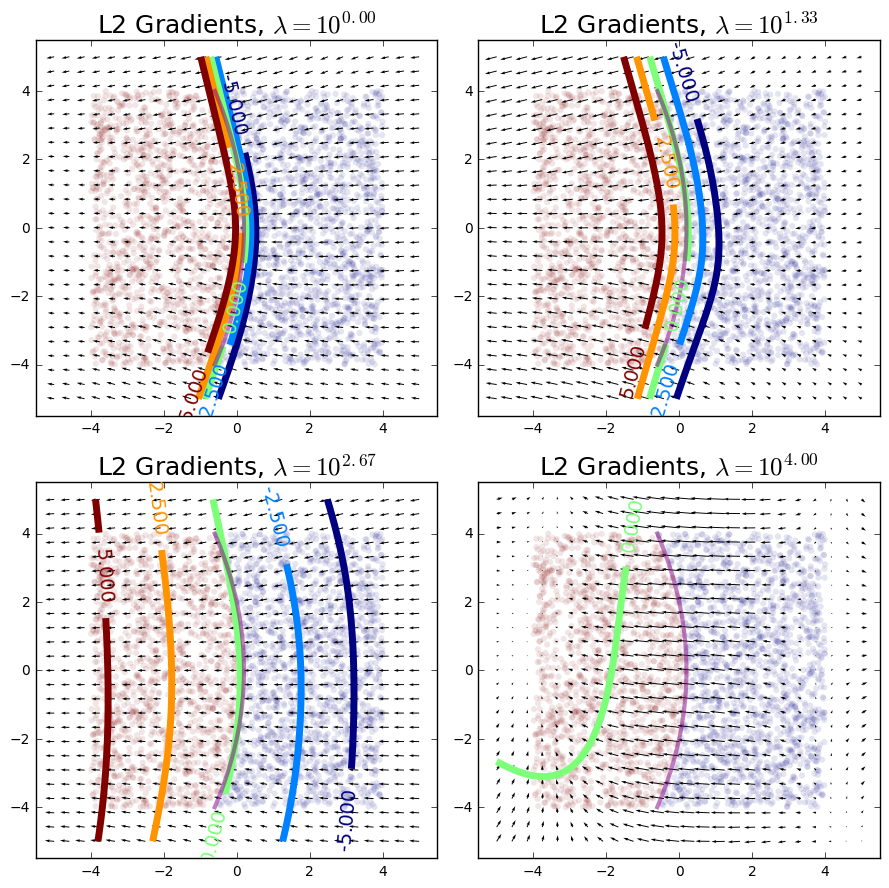
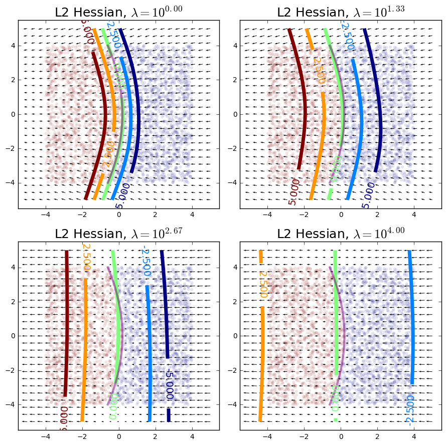
Hessian regularization may be desirable for adversarial robustness and interpretability as well. The results in Figure 2 suggest that exact Hessian regularization for an MLP on a simple 2D problem encourages the model to learn flatter and wider decision boundaries than gradient regularization, which could be useful for interpretability and robustness. Hessian regularization also appears to behave more sensically even when the penalty term is much larger than the cross entropy. By contrast, in this regime, gradient regularization starts pathologically seeking areas of the input space (usually near the edges of the training distribution) where it can set gradients to 0.

Figure 2: Gradient regularization (left) vs. Hessian regularization (right). Purple line indicates the true decision boundary; other lines indicate level sets of a 10-hidden unit MLP’s predicted log-odds from -5 to 5 by increments of 2.5, with the model’s decision boundary in green. Hessian regularization can make decision boundaries wider and flatter without triggering pathological cases.

2 Heftier Surrogates

While input gradient-based methods are appealing because of their close relationship to the shape and curvature of differentiable models’ decision surfaces, they are limited by their locality and humans’ inability to express abstract desiderata in terms of input features. This second limitation in particular prevents us from optimizing for the kind of simplicity or diversity humans find intuitive. Therefore, in the next sections we explore ways of training models using more complex forms of explanation.

One common way of explaining complicated models like neural networks is by distilling them into surrogate models; decision trees are a particularly popular choice Craven and Shavlik (1996). However, these decision trees must sometimes be quite deep in order to accurately explain the associated networks, which defeats the purpose of making predictions interpretable. To address this problem, Wu et al. (2017) optimize the underlying neural networks to be accurately approximatable by shallow decision trees. Performing such an optimization is difficult because the process of distilling a network into a decision tree cannot be expressed analytically, much less differentiated. However, they approximate it by training a second neural network to predict the depth of the decision tree that would result from the first neural network’s parameters. They then use this learned function as a differentiable surrogate of the true approximating decision tree depth. Crucially, they find a depth regime where their networks can outperform decision trees while remaining explainable by them. Although they only try to minimize the approximating decision tree depth, in principle one could train the second network to estimate other characteristics of the decision tree related to simplicity or consistency with domain knowledge (and optimize the main network accordingly).

3 Examples and Exemplars

Another popular way of explaining predictions is with inputs themselves. k-Nearest Neighbors (kNN) algorithms are easy to understand since one can simply present the neighbors, and techniques have recently been proposed to perform kNN using distance metrics derived from pretrained neural networks (Papernot and McDaniel, 2018). More general methods involve sparse graph flows between labeled and unlabeled inputs (Rustamov and Klosowski, 2017) or optimization to find small sets of prototypical inputs that can be used for cluster characterization or classification (Kim et al., 2014), even within neural networks (Li et al., 2017). There has also been recent work on determining which points would most affect a prediction if removed from the training set (Koh and Liang, 2017). These approaches have both advantages and disadvantages. Justifying predictions based on input similarity and difference can seem quite natural, though it can also be confusing or misleading when the metric used to quantify distance between points does not correspond to human intuition. Influence functions shed light on model sensitivities that are otherwise very hard to detect, but they are also very sensitive to outliers, leading to sometimes inscrutable explanations.

However, it seems straightforward at least in principle to implement example-based explanation regularization. For example, we could train neural networks with annotations indicating that certain pairs of examples should be similar or dissimilar, and penalize the model when their intermediate representations are relatively distant or close (which might require altering minibatch sampling to keep paired examples together if annotations are sparse). Although influence functions may be too computationally expensive to incorporate into the loss functions of large networks, it seems useful in principle to specify that certain examples should be particularly representative or influential in deciding how to classify others.

4 Emergent Abstractions

Stepping back, the level of abstraction at which we communicate the reason behind a decision significantly affects its utility, as Keil (2006) notes:

Explanations… suffer if presented at the wrong level of detail. Thus, if asked why John got on the train from New Haven to New York, a good explanation might be that he had tickets for a Broadway show. An accurate but poor explanation at too low a level might say that he got on the train because he moved his right foot from the platform to the train and then followed with his left foot. An accurate but poor explanation at too high a level might say that he got on the train because he believed that the train would take him to New York from New Haven.

The explanations we have considered so far have been in terms of input features, entire inputs, or simple surrogates. However, sometimes humans seek to know the reasons behind predictions at levels of abstraction these forms cannot capture. If we really want to create interpretable interfaces for training and explaining machine learning models, humans and models will need to speak a common language that permits abstraction.

This may seem like a daunting task, but there has been important recent progress in interpreting neural networks in terms of abstractions that emerge during training. Bau et al. (2017) introduce a densely labeled image dataset. They train convolutional neural networks on a top-level classification task, but also include lower-level sublabels that indicate other features in the image. They measure the extent to which different intermediate nodes in their top-level label classifiers serve as exclusive “detectors” for particular sublabels, and compare the extent to which different networks learn different numbers of exclusive detectors. They also categorize their sublabels and look at differences in which kinds of sublabels each network learns to detect (and when these detectors emerge during training).

Kim et al. (2017) provide a method of testing networks’ sensitivity to concepts as defined by user-provided sets of examples. Concretely, they train a simple linear classifer at each layer to distinguish between examples in the concept set and a negative set. They reinterpret the weights of this linear classifier as a “concept activation vector,” and take directional derivatives of the class logits with respect to these concept activations. Repeated across the full dataset for many different concepts, this procedure outputs a set of concept sensitivity weights for each prediction, which can be used for explanation or even image retrieval.

The previous two methods require manual human selection of images corresponding to concepts, and they do not guarantee meaningful correspondence between these concepts and what the network has learned. Feature visualization (Olah et al., 2017) takes a different approach and attempts to understand what the network has learned on its own terms. In particular, it tries to explain what (groups of) neuron(s) learn by optimizing images to maximize (or minimize) their activations. It can also optimize sets of images to jointly maximize activations while encouraging diversity. This process can be useful for obtaining an intuitive sense of (some of) what the model has learned, especially if the neurons being explained are class logits. However, it also leads to an information overload, since modern networks contain millions of neurons and an effectively infinite number of ways to group them. To that end, Olah et al. (2018) use non-negative matrix factorization (NMF) to learn a small number of groups of neurons whose feature visualizations best summarize the entire set. Feature visualizations of neuron groups obtained by NMF tend to correspond more cleanly to human-interpretable concepts, though again there is no guarantee this will occur. Olah et al. (2018) also suggest that incorporating human feedback into this process could lead to a method to train models to make decisions “for the right reasons.”

The above cases either take humans concepts and try to map them to network representations or take network “concepts” and try to visualize them so humans can map them to their own concepts. But they do not actually try to align network representations with human concepts. However, there has been significant recent interest in training models to learn disentangled representations (Chen et al., 2016; Higgins et al., 2016; Siddharth et al., 2017). Disentangled representations are often described as separating out latent factors that concisely characterize important aspects of the inputs but which cannot be easily expressed in terms of their component features. Generally, disentangled representations tend to be much easier to relate to human-intuitive concepts than what models learn when only trained to minimize reconstruction or prediction error.

Figure 3: Accuracies of a normal model and two models trained using find-another-explanation in a disentangled latent space (right) a toy image dataset that confounds background color and square size in training (left) but decouples them in test. Performing find-another-explanation in a latent space allows us to learn models that make predictions for conceptually different reasons, which is reflected in their complementary accuracies on each version of the test set.

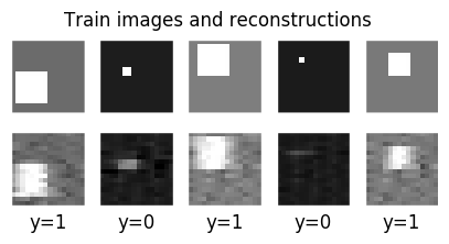
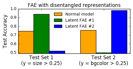
These advances in bridging human and neural representations could have major payoffs in terms of interpreting models or optimizing them to make predictions for specific reasons. Suppose we are interested in testing a classifier’s sensitivity to an abstract concept entangled with our input data. If we have an autoencoder whose representation of the input disentangles the concept into a small set of latent factors, then for a specific input, we can encode it, decode it, and pass the decoded input through the classifier, taking the gradient of the network’s output with respect to the latent factors associated with the concept. If we fix the autoencoder weights but not the classifier weights, we can use this differentiable concept sensitivity score to apply our “right for the right reasons” technique from Chapter 1 to encourage the classifier to be sensitive or insensitive to the concept.

We present a preliminary proof of concept of this idea in Figure 3. In this experiment, we construct a toy dataset of images of white squares with four true latent factors of variation: the size of the square, its x and y position, and the background color of the image. In training, background color and square size are confounded; images either have dark backgrounds and small squares or light backgrounds and large squares (and either one can be used to predict the label). However, we create two versions of the test set where these latent factors are decoupled (and only one predicts the label). This is analogous to the parable in our introduction with squares representing tanks and background colors representing light. When we train a one-hidden layer MLP normally, it learns to implicitly use both factors, and obtains suboptimal accuracies of about 75% on each test set. To circumvent this issue, we first train a convolutional autoencoder that disentangles square size from background color (which we do with supervision here, but in principle this can be unsupervised) and then prepend the autoencoder to our MLP with fixed weights. We then simultaneously train two instantiations of this network with the find-another-explanation penalty we introduced in Section 1.C. These two networks learn to perform nearly perfectly on one test set and do no better than random guessing on the other, which suggests they are making predictions for different conceptual reasons. Obtaining these networks would have been very difficult using only gradient penalties in the input space.

5 Interpretability Interfaces

Olah et al. (2018) describe a space of “interpretability interfaces” and introduce a formal grammar for expressing explanations of neural networks (and a systematic way of exploring designs). They visualize this design space in a grid of relationships between different “substrates” of the design, which include groups of neurons, dataset examples, and model parameters – the latter of which presents an opportunity “to consider interfaces for taking action in neural networks.” If human-defined concepts, disentangled representations, or other forms of explanation are included as additional substrates, one can start to imagine a very general framework for expressing priors or constraints on relationships between them. These would be equivalent to optimizing models to make predictions for specific reasons.

Figure 4: Schematic diagram of an interpretability interface.

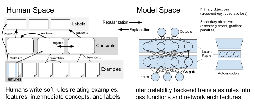
How would humans actually express these kinds of objectives? One interface worth emulating could be that introduced by recent but popular libraries for weak supervision (Ratner et al., 2017) or probabilistic soft logic (Bach et al., 2017), which is related to the well-studied topic of fuzzy logic, a method noted for its compatibility with human reasoning (Zadeh, 1997). In these frameworks, users can specify “soft” logical rules for labeling datasets or constraining relationships between atoms (or substrates) of a system. Though users can sometimes specify that certain rules are inviolable or highly-weighted, in general these systems assume that rules are not always correct and attempt to infer weights for each. While these inference problems are nontrivial, and in general there may be complex, structured interactions between rules that are difficult to capture, the interface it exposes to users is expressive and potentially worth emulating in an interpretability interface. For example, we could imagine writing soft rules relating:

• dataset examples to each other (e.g. these examples should be conceptually similar with respect to a task)

• dataset examples to concepts (e.g. these are examples of a concept)

• features to concepts (e.g. this set of features is related to this concept, this other set is not; in this specific case, these features contribute positively)

• concepts to predictions (e.g. the presence of this concept makes this prediction more or less likely, except when this other concept is present)

These rules could be “compiled” into additional energy terms in the model’s loss function, possibly with thresholding if we expect them to be incorrect some percentage of the time (though rules defined for specific examples may be more reliable). We present a schematic diagram of how a system like this might work in Figure 4.

Such a system would strongly depend on being able to define rules in terms of abstract concepts, but such rules might not be enforcible until the model has a differentiable, stable representations of them. However, one could imagine pre-learning static, disentangled concept representations that could be related back to input features. If 1:1 mappings between human concepts and latent representations do not emerge naturally, even allowing for hierarchical relationships (Esmaeili et al., 2018), steps could be taken to optimize model representations to better match human understanding (e.g. using partial supervision) or to help humans better understand model representations (e.g. using feature visualization). This process of reaching user-model intersubjectivity might require multiple stages of identification and refinement, but seems possible in principle. And perhaps arriving at a shared conceptual framework for understanding a problem is where the work of teaching and learning ought to lie, regardless of whether the teachers and learners are human.

6 Discussion

In this chapter, we discussed a number of strategies for explanation regularization beyond the methods we used in the previous chapters. We described simple extensions of gradient-based methods (imposing L1 and Hessian penalties), strategies in terms of interpretable surrogates (regularizing distilled decision trees, nearest neighbors, and exemplars), and strategies in terms of concepts (concept activation vectors, disentangled representations, and feature visualization). We then combined many of these strategies into a design for an “interpretability interface” that could be used to simultaneously improve neural network interpretability and incorporate domain knowledge.

One limitation of this discussion is that we only considered classification models and traditional ways of explaining their predictions. However, there is a much larger literature on alternative forms of explanation and prediction like intuitive theories (Gerstenberg and Tenenbaum, 2017) or causal inference (Pearl, 2010) that is highly relevant, especially if we want to apply these techniques to problems like sequential decisionmaking. We started this thesis by making a point that was “easiest to express with a story;” even with arbitrarily human-friendly compositional abstraction (Schulz et al., 2017), flat sets of concepts may never be sufficient in cases where users think in terms of narratives (Abell, 2004).

However, despite these limitations, we think the works we have outlined in this chapter have started to map a rich design space for interpreting and training machine learning models with more than just $x$es and $y$s.

Chapter 4 Conclusion

Building on Keil (2006), Doshi-Velez and Kim (2017) argue that explanations are necessary when our models have a certain incompleteness. In the context of this thesis, we have considered the kind of incompleteness that results from ambiguity in a dataset. When datasets do not fully specify their decision boundaries, we have freedom to learn many models that could accurately classify them. We generate explanations to determine which model we learned; we regularize explanations to choose which model to learn.

In Chapter 1, we provided our first formulation of explanation regularization using input gradients, a particular kind of local explanation that is low-level but faithful and differentiable. We then used this method to solve classification problems despite the presence of challenging confounding factors, find diverse solutions, and achieve high accuracy with significantly fewer training examples. In Chapter 2, we applied explanation regularization to CNN saliency maps and showed we could make our CNNs both more interpretable and more robust to adversarial attacks. In both chapters, we found that explanations were reliable indicators of generalizability. In Chapter 3, we reviewed other potential ways of implementing explanation regularization, including penalties based on alternative gradient penalties, complex surrogates, nearest neighbors, and even abstract concepts (realized via disentangled representations). Finally, we presented a vision for an interface that would allow users and machine learning models to explain predictions to each other, using a common conceptual framework they define together.

One methodological point we would like to stress before closing is about the importance of ground truth in evaluating explanation techniques. Throughout this thesis, we tried to ensure that whenever we evaluated explanations, we also had some way of determining what those explanations should be. For example, in Chapter 1, we knew which features in our synthetic dataset actually mattered for prediction, and we knew that models fooled by decoy datasets were sensitive to the corresponding confounds. Regardless of whether explanations are used in human-, application-, or functionally-grounded tasks (Doshi-Velez and Kim, 2017), having ground truth is critical – especially given recent criticisms of many explanation methods for being unhelpful in detecting generalization issues (Chandrasekaran et al., 2017), being sensitive to meaningless changes to models (Kindermans et al., 2017; Ghorbani et al., 2017), or being invariant to meaningful changes to models (Adebayo et al., 2018). Otherwise, we may end up rationalizing our predictions rather than explaining them.

Machine learning is being deployed in more and more critical domains, including the automotive industry, medicine, lending, bail determination (Angwin et al., 2016), and even child maltreatment hotlines (Chouldechova et al., 2018). As we move forward, it is essential that we develop better diagnostic tools for understanding when our models are wrong and how to right them. The promise of machine learning to improve human lives is great, but so is its peril. To use machine learning models responsibly, regardless of whether they seem right, we must have methods of making sure they are reasonable.

References

- Abell (2004) Abell, P. (2004). Narrative explanation: an alternative to variable-centered explanation? Annu. Rev. Sociol., 30, 287–310.
- Adebayo et al. (2018) Adebayo, J., Gilmer, J., Goodfellow, I. and Kim, B. (2018). Local explanation methods for deep neural networks lack sensitivity to parameter values.
- Angwin et al. (2016) Angwin, J., Larson, J., Mattu, S. and Kirchner, L. (2016). How we analyzed the compas recidivism algorithm. ProPublica.
- Athalye and Sutskever (2017) Athalye, A. and Sutskever, I. (2017). Synthesizing robust adversarial examples. arXiv preprint arXiv:1707.07397.
- Ba and Caruana (2014) Ba, J. and Caruana, R. (2014). Do deep nets really need to be deep? In Advances in neural information processing systems, pp. 2654–2662.
- Bach et al. (2015) Bach, S., Binder, A., Montavon, G., Klauschen, F., Müller, K.-R. and Samek, W. (2015). On pixel-wise explanations for non-linear classifier decisions by layer-wise relevance propagation. PloS one, 10 (7), e0130140.
- Bach et al. (2017) Bach, S. H., Broecheler, M., Huang, B. and Getoor, L. (2017). Hinge-loss markov random fields and probabilistic soft logic. Journal of Machine Learning Research, 18 (109), 1–67.
- Baehrens et al. (2010) Baehrens, D., Schroeter, T., Harmeling, S., Kawanabe, M., Hansen, K. and MÞller, K.-R. (2010). How to explain individual classification decisions. Journal of Machine Learning Research, 11 (Jun), 1803–1831.
- Barber (2012) Barber, D. (2012). Bayesian reasoning and machine learning. Cambridge University Press.
- Bau et al. (2017) Bau, D., Zhou, B., Khosla, A., Oliva, A. and Torralba, A. (2017). Network dissection: Quantifying interpretability of deep visual representations. In Computer Vision and Pattern Recognition (CVPR), 2017 IEEE Conference on, IEEE, pp. 3319–3327.
- Bishop (1993) Bishop, C. M. (1993). Curvature-driven smoothing: a learning algorithm for feedforward networks. IEEE Transactions on Neural Networks, 4 (5), 882–884.
- Butalov (2011) Butalov, Y. (2011). The notMNIST dataset. http://yaroslavvb.com/upload/notMNIST/.
- Carlini and Wagner (2016) Carlini, N. and Wagner, D. (2016). Defensive distillation is not robust to adversarial examples. arXiv preprint arXiv:1607.04311.
- Caruana et al. (2015) Caruana, R., Lou, Y., Gehrke, J., Koch, P., Sturm, M. and Elhadad, N. (2015). Intelligible models for healthcare: Predicting pneumonia risk and hospital 30-day readmission. In Proceedings of the 21th ACM SIGKDD International Conference on Knowledge Discovery and Data Mining, ACM, pp. 1721–1730.
- Chandrasekaran et al. (2017) Chandrasekaran, A., Yadav, D., Chattopadhyay, P., Prabhu, V. and Parikh, D. (2017). It takes two to tango: Towards theory of ai’s mind. arXiv preprint arXiv:1704.00717.
- Chen et al. (2016) Chen, X., Duan, Y., Houthooft, R., Schulman, J., Sutskever, I. and Abbeel, P. (2016). Infogan: Interpretable representation learning by information maximizing generative adversarial nets. In Advances in Neural Information Processing Systems, pp. 2172–2180.
- Chouldechova et al. (2018) Chouldechova, A., Benavides-Prado, D., Fialko, O. and Vaithianathan, R. (2018). A case study of algorithm-assisted decision making in child maltreatment hotline screening decisions. In S. A. Friedler and C. Wilson (eds.), Proceedings of the 1st Conference on Fairness, Accountability and Transparency, New York, NY, USA: PMLR, Proceedings of Machine Learning Research, vol. 81, pp. 134–148.
- Craven and Shavlik (1996) Craven, M. and Shavlik, J. W. (1996). Extracting tree-structured representations of trained networks. In Advances in neural information processing systems, pp. 24–30.
- Czarnecki et al. (2017) Czarnecki, W. M., Osindero, S., Jaderberg, M., Swirszcz, G. and Pascanu, R. (2017). Sobolev training for neural networks. In Advances in Neural Information Processing Systems, pp. 4281–4290.
- Donahue and Grauman (2011) Donahue, J. and Grauman, K. (2011). Annotator rationales for visual recognition. In 2011 International Conference on Computer Vision, IEEE, pp. 1395–1402.
- Doshi-Velez and Kim (2017) Doshi-Velez, F. and Kim, B. (2017). Towards a rigorous science of interpretable machine learning. arXiv preprint arXiv:1702.08608.
- Dreyfus and Dreyfus (1992) Dreyfus, H. L. and Dreyfus, S. E. (1992). What artificial experts can and cannot do. AI & society, 6 (1), 18–26.
- Drucker and Le Cun (1992) Drucker, H. and Le Cun, Y. (1992). Improving generalization performance using double backpropagation. IEEE Transactions on Neural Networks, 3 (6), 991–997.
- Esmaeili et al. (2018) Esmaeili, B., Wu, H., Jain, S., Narayanaswamy, S., Paige, B. and van de Meent, J.-W. (2018). Hierarchical disentangled representations. arXiv preprint arXiv:1804.02086.
- Fong and Vedaldi (2017) Fong, R. and Vedaldi, A. (2017). Interpretable explanations of black boxes by meaningful perturbation. arXiv preprint arXiv:1704.03296.
- Gerstenberg and Tenenbaum (2017) Gerstenberg, T. and Tenenbaum, J. B. (2017). Intuitive theories. Oxford handbook of causal reasoning, pp. 515–548.
- Ghorbani et al. (2017) Ghorbani, A., Abid, A. and Zou, J. (2017). Interpretation of neural networks is fragile. arXiv preprint arXiv:1710.10547.
- Goodfellow et al. (2014) Goodfellow, I. J., Shlens, J. and Szegedy, C. (2014). Explaining and harnessing adversarial examples. arXiv preprint arXiv:1412.6572.
- Grundland and Dodgson (2007) Grundland, M. and Dodgson, N. A. (2007). Decolorize: Fast, contrast enhancing, color to grayscale conversion. Pattern Recognition, 40 (11), 2891–2896.
- Gu and Rigazio (2014) Gu, S. and Rigazio, L. (2014). Towards deep neural network architectures robust to adversarial examples. arXiv preprint arXiv:1412.5068.
- Hechtlinger (2016) Hechtlinger, Y. (2016). Interpretation of prediction models using the input gradient. arXiv preprint arXiv:1611.07634.
- Hein and Andriushchenko (2017) Hein, M. and Andriushchenko, M. (2017). Formal guarantees on the robustness of a classifier against adversarial manipulation. In Advances in Neural Information Processing Systems, pp. 2263–2273.
- Higgins et al. (2016) Higgins, I., Matthey, L., Pal, A., Burgess, C., Glorot, X., Botvinick, M., Mohamed, S. and Lerchner, A. (2016). beta-vae: Learning basic visual concepts with a constrained variational framework.
- Kang and Kang (2017) Kang, H.-W. and Kang, H.-B. (2017). Prediction of crime occurrence from multi-modal data using deep learning. PloS one, 12 (4), e0176244.
- Keil (2006) Keil, F. C. (2006). Explanation and understanding. Annu. Rev. Psychol., 57, 227–254.
- Kim et al. (2017) Kim, B., Gilmer, J., Viegas, F., Erlingsson, U. and Wattenberg, M. (2017). Tcav: Relative concept importance testing with linear concept activation vectors. arXiv preprint arXiv:1711.11279.
- Kim et al. (2014) —, Rudin, C. and Shah, J. A. (2014). The bayesian case model: A generative approach for case-based reasoning and prototype classification. In Advances in Neural Information Processing Systems, pp. 1952–1960.
- Kindermans et al. (2017) Kindermans, P.-J., Hooker, S., Adebayo, J., Alber, M., Schütt, K. T., Dähne, S., Erhan, D. and Kim, B. (2017). The (un) reliability of saliency methods. arXiv preprint arXiv:1711.00867.
- Kingma and Ba (2014) Kingma, D. and Ba, J. (2014). Adam: A method for stochastic optimization. arXiv preprint arXiv:1412.6980.
- Koh and Liang (2017) Koh, P. W. and Liang, P. (2017). Understanding black-box predictions via influence functions. In International Conference on Machine Learning, pp. 1885–1894.
- Kurakin et al. (2016a) Kurakin, A., Goodfellow, I. and Bengio, S. (2016a). Adversarial examples in the physical world. arXiv preprint arXiv:1607.02533.
- Kurakin et al. (2016b) —, — and — (2016b). Adversarial machine learning at scale. arXiv preprint arXiv:1611.01236.
- LeCun et al. (2010) LeCun, Y., Cortes, C. and Burges, C. J. (2010). The MNIST database of handwritten digits. http://yann.lecun.com/exdb/mnist/.
- Lei et al. (2016) Lei, T., Barzilay, R. and Jaakkola, T. (2016). Rationalizing neural predictions. arXiv preprint arXiv:1606.04155.
- Li et al. (2015) Li, J., Chen, X., Hovy, E. and Jurafsky, D. (2015). Visualizing and understanding neural models in NLP. arXiv preprint arXiv:1506.01066.
- Li et al. (2016) —, Monroe, W. and Jurafsky, D. (2016). Understanding neural networks through representation erasure. arXiv preprint arXiv:1612.08220.
- Li et al. (2017) Li, O., Liu, H., Chen, C. and Rudin, C. (2017). Deep learning for case-based reasoning through prototypes: A neural network that explains its predictions. arXiv preprint arXiv:1710.04806.
- Lichman (2013) Lichman, M. (2013). UCI machine learning repository. http://archive.ics.uci.edu/ml.
- Lipton (2016) Lipton, Z. C. (2016). The mythos of model interpretability. CoRR, abs/1606.03490.
- Lundberg and Lee (2016) Lundberg, S. and Lee, S.-I. (2016). An unexpected unity among methods for interpreting model predictions. arXiv preprint arXiv:1611.07478.
- Mclaurin et al. (2017) Mclaurin, D., Duvenaud, D. and Johnson, M. (2017). Autograd. https://github.com/HIPS/autograd.
- Montavon et al. (2017) Montavon, G., Lapuschkin, S., Binder, A., Samek, W. and Müller, K.-R. (2017). Explaining nonlinear classification decisions with deep taylor decomposition. Pattern Recognition, 65, 211–222.
- Nayebi and Ganguli (2017) Nayebi, A. and Ganguli, S. (2017). Biologically inspired protection of deep networks from adversarial attacks. arXiv preprint arXiv:1703.09202.
- Netzer et al. (2011) Netzer, Y., Wang, T., Coates, A., Bissacco, A., Wu, B. and Ng, A. Y. (2011). Reading digits in natural images with unsupervised feature learning. In NIPS Workshop on Deep Learning and Unsupervised Feature Learning 2011.
- Olah et al. (2017) Olah, C., Mordvintsev, A. and Schubert, L. (2017). Feature visualization. Distill, https://distill.pub/2017/feature-visualization.
- Olah et al. (2018) —, Satyanarayan, A., Johnson, I., Carter, S., Schubert, L., Ye, K. and Mordvintsev, A. (2018). The building blocks of interpretability. Distill, https://distill.pub/2018/building-blocks.
- Papernot et al. (2016a) Papernot, N., Goodfellow, I., Sheatsley, R., Feinman, R. and McDaniel, P. (2016a). cleverhans v1.0.0: an adversarial machine learning library. arXiv preprint arXiv:1610.00768.
- Papernot and McDaniel (2018) — and McDaniel, P. (2018). Deep k-nearest neighbors: Towards confident, interpretable and robust deep learning. arXiv preprint arXiv:1803.04765.
- Papernot et al. (2017) —, —, Goodfellow, I., Jha, S., Celik, Z. B. and Swami, A. (2017). Practical black-box attacks against machine learning. In Proceedings of the 2017 ACM on Asia Conference on Computer and Communications Security, ACM, pp. 506–519.
- Papernot et al. (2016b) —, —, Jha, S., Fredrikson, M., Celik, Z. B. and Swami, A. (2016b). The limitations of deep learning in adversarial settings. In Security and Privacy (EuroS&P), 2016 IEEE European Symposium on, IEEE, pp. 372–387.
- Papernot et al. (2016c) —, —, Wu, X., Jha, S. and Swami, A. (2016c). Distillation as a defense to adversarial perturbations against deep neural networks. In Security and Privacy (SP), 2016 IEEE Symposium on, IEEE, pp. 582–597.
- Pearl (2010) Pearl, J. (2010). Causal inference. In Causality: Objectives and Assessment, pp. 39–58.
- Raghunathan et al. (2018) Raghunathan, A., Steinhardt, J. and Liang, P. (2018). Certified defenses against adversarial examples. arXiv preprint arXiv:1801.09344.
- Ratner et al. (2017) Ratner, A., Bach, S. H., Ehrenberg, H., Fries, J., Wu, S. and Ré, C. (2017). Snorkel: Rapid training data creation with weak supervision. arXiv preprint arXiv:1711.10160.
- Ribeiro (2016) Ribeiro, M. T. (2016). LIME. https://github.com/marcotcr/lime.
- Ribeiro et al. (2016) —, Singh, S. and Guestrin, C. (2016). Why should I trust you?: Explaining the predictions of any classifier. In Proceedings of the 22nd ACM SIGKDD International Conference on Knowledge Discovery and Data Mining, ACM, pp. 1135–1144.
- Rifai et al. (2011) Rifai, S., Mesnil, G., Vincent, P., Muller, X., Bengio, Y., Dauphin, Y. and Glorot, X. (2011). Higher order contractive auto-encoder. In Joint European Conference on Machine Learning and Knowledge Discovery in Databases, Springer, pp. 645–660.
- Ross and Doshi-Velez (2018) Ross, A. and Doshi-Velez, F. (2018). Improving the adversarial robustness and interpretability of deep neural networks by regularizing their input gradients. In Proceedings of the Thirty-Second AAAI Conference on Artificial Intelligence.
- Ross et al. (2017a) —, Lage, I. and Doshi-Velez, F. (2017a). The neural lasso: Local linear sparsity for interpretable explanations. In Workshop on Transparent and Interpretable Machine Learning in Safety Critical Environments, 31st Conference on Neural Information Processing Systems, https://goo.gl/TwRhXo.
- Ross et al. (2017b) Ross, A. S., Hughes, M. C. and Doshi-Velez, F. (2017b). Right for the right reasons: Training differentiable models by constraining their explanations. In Proceedings of the Twenty-Sixth International Joint Conference on Artificial Intelligence, pp. 2662–2670.
- Rustamov and Klosowski (2017) Rustamov, R. M. and Klosowski, J. T. (2017). Interpretable graph-based semi-supervised learning via flows. arXiv preprint arXiv:1709.04764.
- Schulz et al. (2017) Schulz, E., Tenenbaum, J. B., Duvenaud, D., Speekenbrink, M. and Gershman, S. J. (2017). Compositional inductive biases in function learning. Cognitive psychology, 99, 44–79.
- Selvaraju et al. (2016) Selvaraju, R. R., Das, A., Vedantam, R., Cogswell, M., Parikh, D. and Batra, D. (2016). Grad-CAM: Why did you say that? arXiv preprint arXiv:1611.07450.
- Sermanet et al. (2012) Sermanet, P., Chintala, S. and LeCun, Y. (2012). Convolutional neural networks applied to house numbers digit classification. In Pattern Recognition (ICPR), 2012 21st International Conference on, IEEE, pp. 3288–3291.
- Shrikumar et al. (2016) Shrikumar, A., Greenside, P., Shcherbina, A. and Kundaje, A. (2016). Not just a black box: Learning important features through propagating activation differences. arXiv preprint arXiv:1605.01713.
- Siddharth et al. (2017) Siddharth, N., Paige, B., Van de Meent, J.-W., Desmaison, A. and Torr, P. H. (2017). Learning disentangled representations with semi-supervised deep generative models.
- Simonyan et al. (2013) Simonyan, K., Vedaldi, A. and Zisserman, A. (2013). Deep inside convolutional networks: Visualising image classification models and saliency maps. arXiv preprint arXiv:1312.6034.
- Singh et al. (2016) Singh, S., Ribeiro, M. T. and Guestrin, C. (2016). Programs as black-box explanations. arXiv preprint arXiv:1611.07579.
- Smilkov et al. (2017) Smilkov, D., Thorat, N., Kim, B., Viégas, F. and Wattenberg, M. (2017). Smoothgrad: removing noise by adding noise. arXiv preprint arXiv:1706.03825.
- Sundararajan et al. (2017) Sundararajan, M., Taly, A. and Yan, Q. (2017). Axiomatic attribution for deep networks. arXiv preprint arXiv:1703.01365.
- Szegedy et al. (2013) Szegedy, C., Zaremba, W., Sutskever, I., Bruna, J., Erhan, D., Goodfellow, I. and Fergus, R. (2013). Intriguing properties of neural networks. arXiv preprint arXiv:1312.6199.
- Tramèr et al. (2017a) Tramèr, F., Kurakin, A., Papernot, N., Boneh, D. and McDaniel, P. (2017a). Ensemble adversarial training: Attacks and defenses. arXiv preprint arXiv:1705.07204.
- Tramèr et al. (2017b) —, Papernot, N., Goodfellow, I., Boneh, D. and McDaniel, P. (2017b). The space of transferable adversarial examples. arXiv preprint arXiv:1704.03453.
- Wu et al. (2017) Wu, M., Hughes, M. C., Parbhoo, S., Zazzi, M., Roth, V. and Doshi-Velez, F. (2017). Beyond sparsity: Tree regularization of deep models for interpretability. arXiv preprint arXiv:1711.06178.
- Xu et al. (2017) Xu, W., Evans, D. and Qi, Y. (2017). Feature squeezing: Detecting adversarial examples in deep neural networks. arXiv preprint arXiv:1704.01155.
- Zadeh (1997) Zadeh, L. A. (1997). Toward a theory of fuzzy information granulation and its centrality in human reasoning and fuzzy logic. Fuzzy sets and systems, 90 (2), 111–127.
- Zaidan et al. (2007) Zaidan, O., Eisner, J. and Piatko, C. D. (2007). Using "annotator rationales" to improve machine learning for text categorization. In HLT-NAACL, Citeseer, pp. 260–267.
- Zeiler and Fergus (2014) Zeiler, M. D. and Fergus, R. (2014). Visualizing and understanding convolutional networks. In European conference on computer vision, Springer, pp. 818–833.
- Zhang et al. (2016) Zhang, Y., Marshall, I. and Wallace, B. C. (2016). Rationale-augmented convolutional neural networks for text classification. arXiv preprint arXiv:1605.04469.