Raster Grid Pathology and the Cure

Albert Fannjiang Department of Mathematics, University of California, Davis, California 95616, USA. Email: fannjiang@math.ucdavis.edu
Abstract.

Blind ptychography is a phase retrieval method using multiple coded diffraction patterns from different, overlapping parts of the unknown extended object illuminated with an unknown window function. The window function is also known as the probe in the optics literature. As such blind ptychography is an inverse problem of simultaneous recovery of the object and the window function given the intensities of the windowed Fourier transform and has a multi-scale set-up in which the probe has an intermediate scale between the pixel scale and the macro-scale of the extended object. Uniqueness problem for blind ptychography is analyzed rigorously for the raster scan (of a constant step size τ𝜏\tau) and its variants, in which another scale comes into play: the overlap between adjacent blocks (the shifted windows). The block phases are shown to form an arithmetic progression and the complete characterization of the raster scan ambiguities is given, including: First, the periodic raster grid pathology of degrees of freedom proportional to τ2superscript𝜏2\tau^{2} and, second, a non-periodic, arithmetically progressing phase shift from block to block. Finally irregularly perturbed raster scans are shown to remove all ambiguities other than the inherent ambiguities of the scaling factor and the affine phase ambiguity under the minimum requirement of roughly 50%percent5050\% overlap ratio.

1. Introduction

In the last decade, ptychography has made rapid technological advances and developed into a powerful lensless coherent imaging method [37, 19, 41]. Ptychography collects the diffraction patterns from overlapping illuminations of various parts of the unknown object using a localized coherent source (the probe) [31, 28, 32], and builds on the advances in synthetic aperture methods to extend phase retrieval to unlimited objects and enhance imaging resolution [30, 26, 27, 20, 6]. Blind ptychography goes a step further and seeks to reconstruct both the unknown object and the unknown probe simultaneously [36, 29].

Mathematically, blind ptychography is an inverse problem of simultaneous recovery of the object and the window function (the probe) given the intensities of the windowed Fourier transform. In ptychography, the window function has an intermediate scale between the pixel scale and the macro-scale of the extended object.

The performance of ptychography depends on factors such as the type of illumination and the measurement scheme, including the amounts of overlap and probe positions. For example, the use of randomly structured illuminations can improve ptychographic reconstruction over that with regular illuminations [39, 40, 35, 34, 33, 30, 22, 17, 9, 12, 4, 11, 8]. Experiments suggest an overlap ratio of at least 50%, typically 60-70% between adjacent illuminations for blind ptychography [3, 23]. Optimizing the scan pattern can significantly improve the performance of ptychography and is an important part of the experimental design.

In particular, empirical evidences repeatedly point to the pitfalls of the raster scan, which is experimentally the easiest to implement [15]. Mathematically speaking, blind ptychography with raster scan seeks to recover both the object and the window function (the probe) as unknowns but only the 2D windowed Fourier intensities (coded diffraction patterns) as the data. Raster scanning refers to the positions of the window function. The raster scan scheme is susceptible to periodic artifacts, known as raster grid pathology, attributed to the regularity and symmetry of the scan positions [36].

On the other hand, to the best of our knowledge, raster grid pathology has not be precisely formulated and analyzed. The purpose of the present work is a complete analysis of raster grid pathology from the perspective of inverse problems. Uniqueness of solution is fundamental to any inverse problem. The exceptions to uniqueness are called the ambiguities. We identify the rater grid pathology reported in optics literature as periodic ambiguities of period equal to the step size of the raster scan. Moreover, we will characterize all the ambiguities inherent to the raster scan ptychography and propose a simple modification that can eliminate all the ambiguities except for those inherent to any blind ptychography.

The first thing to note is that raster grid pathology only appears in blind ptychography but not in ptychography with a known probe. In the latter case, the only ambiguity is a constant phase factor which has no real significance (and will be ignored) and the convergence behaviors of the raster scan ptychography with a known probe has been rigorously established [4].

Second, there are two ambiguities inherent to any blind ptychography: a scaling factor and an affine phase factor. To give a precise description, we introduce some notation as follows.

Let n2=0,n12superscriptsubscript𝑛2superscript0𝑛12\mathbb{Z}_{n}^{2}=\llbracket 0,n-1\rrbracket^{2} be the object domain containing the support of the discrete object f𝑓f where k,l𝑘𝑙\llbracket k,l\rrbracket denotes the integers between, and including, kl𝑘𝑙k\leq l\in\mathbb{Z}. Let 00:=m2,m<n,formulae-sequenceassignsuperscript00superscriptsubscript𝑚2𝑚𝑛{\mathcal{M}}^{00}:=\mathbb{Z}_{m}^{2},m<n, be the initial probe area which is also the support of the probe μ00superscript𝜇00\mu^{00} describing the illumination field. Here n𝑛n is the global scale and m𝑚m the intermediate scale of the set-up.

Let 𝒯𝒯{\mathcal{T}} be the set of all shifts, including (0,0)00(0,0), involved in the ptychographic measurement. Denote by μ𝐭superscript𝜇𝐭\mu^{\mathbf{t}} the 𝐭𝐭\mathbf{t}-shifted probe for all 𝐭𝒯𝐭𝒯\mathbf{t}\in{\mathcal{T}} and 𝐭superscript𝐭{\mathcal{M}}^{\mathbf{t}} the domain of μ𝐭superscript𝜇𝐭\mu^{\mathbf{t}}. Let f𝐭superscript𝑓𝐭f^{\mathbf{t}} the object restricted to 𝐭superscript𝐭{\mathcal{M}}^{\mathbf{t}}. We write f=𝐭f𝐭𝑓subscript𝐭superscript𝑓𝐭f=\vee_{\mathbf{t}}f^{\mathbf{t}} and refer to each f𝐭superscript𝑓𝐭f^{\mathbf{t}} as a part of f𝑓f. In ptychography, the original object is broken up into a set of overlapping object parts, each of which produces a μ𝐭superscript𝜇𝐭\mu^{\mathbf{t}}-coded diffraction pattern (i.e. Fourier intensity). The totality of the coded diffraction patterns is called the ptychographic measurement data. Let ν00superscript𝜈00\nu^{00} (with 𝐭=(0,0)𝐭00\mathbf{t}=(0,0)) and g=𝐭g𝐭𝑔subscript𝐭superscript𝑔𝐭g=\vee_{\mathbf{t}}g^{\mathbf{t}} be any pair of the probe and the object estimates producing the same ptychography data as μ00superscript𝜇00\mu^{00} and f𝑓f, i.e. the diffraction pattern of ν𝐭g𝐭direct-productsuperscript𝜈𝐭superscript𝑔𝐭\nu^{\mathbf{t}}\odot g^{\mathbf{t}} is identical to that of μ𝐭f𝐭direct-productsuperscript𝜇𝐭superscript𝑓𝐭\mu^{\mathbf{t}}\odot f^{\mathbf{t}} where ν𝐭superscript𝜈𝐭\nu^{\mathbf{t}} is the 𝐭𝐭\mathbf{t}-shift of ν00superscript𝜈00\nu^{00} and g𝐭superscript𝑔𝐭g^{\mathbf{t}} is the restriction of g𝑔g to 𝐭superscript𝐭{\mathcal{M}}^{\mathbf{t}}. For convenience, we assume the value zero for μ𝐭,f𝐭,ν𝐭,g𝐭superscript𝜇𝐭superscript𝑓𝐭superscript𝜈𝐭superscript𝑔𝐭\mu^{\mathbf{t}},f^{\mathbf{t}},\nu^{\mathbf{t}},g^{\mathbf{t}} outside of 𝐭superscript𝐭{\mathcal{M}}^{\mathbf{t}} and the periodic boundary condition on n2superscriptsubscript𝑛2\mathbb{Z}_{n}^{2} when μ𝐭superscript𝜇𝐭\mu^{\mathbf{t}} crosses over the boundary of n2superscriptsubscript𝑛2\mathbb{Z}_{n}^{2}.

Consider the probe and object estimates

(1) ν00(𝐧)superscript𝜈00𝐧\displaystyle\nu^{00}({\mathbf{n}}) =\displaystyle= μ00(𝐧)exp(iai𝐰𝐧),𝐧00superscript𝜇00𝐧i𝑎i𝐰𝐧𝐧superscript00\displaystyle\mu^{00}({\mathbf{n}})\exp(-{\rm i}a-{\rm i}\mathbf{w}\cdot{\mathbf{n}}),\quad{\mathbf{n}}\in{\mathcal{M}}^{00}
(2) g(𝐧)𝑔𝐧\displaystyle g({\mathbf{n}}) =\displaystyle= f(𝐧)exp(ib+i𝐰𝐧),𝐧n2𝑓𝐧i𝑏i𝐰𝐧𝐧subscriptsuperscript2𝑛\displaystyle f({\mathbf{n}})\exp({\rm i}b+{\rm i}\mathbf{w}\cdot{\mathbf{n}}),\quad{\mathbf{n}}\in\mathbb{Z}^{2}_{n}

for any a,b𝑎𝑏a,b\in\mathbb{R} and 𝐰2𝐰superscript2\mathbf{w}\in\mathbb{R}^{2}. For any 𝐭𝐭\mathbf{t}, we have the following calculation

ν𝐭(𝐧)superscript𝜈𝐭𝐧\displaystyle\nu^{\mathbf{t}}({\mathbf{n}}) =\displaystyle= ν00(𝐧𝐭)superscript𝜈00𝐧𝐭\displaystyle\nu^{00}({\mathbf{n}}-\mathbf{t})
=\displaystyle= μ00(𝐧𝐭)exp(i𝐰(𝐧𝐭))exp(ia)superscript𝜇00𝐧𝐭i𝐰𝐧𝐭i𝑎\displaystyle\mu^{00}({\mathbf{n}}-\mathbf{t})\exp(-{\rm i}\mathbf{w}\cdot({\mathbf{n}}-\mathbf{t}))\exp(-{\rm i}a)
=\displaystyle= μ𝐭(𝐧)exp(i𝐰(𝐧𝐭))exp(ia)superscript𝜇𝐭𝐧i𝐰𝐧𝐭i𝑎\displaystyle\mu^{\mathbf{t}}({\mathbf{n}})\exp(-{\rm i}\mathbf{w}\cdot({\mathbf{n}}-\mathbf{t}))\exp(-{\rm i}a)

and hence for all 𝐧𝐭,𝐭𝒯formulae-sequence𝐧superscript𝐭𝐭𝒯{\mathbf{n}}\in{\mathcal{M}}^{\mathbf{t}},\mathbf{t}\in{\mathcal{T}}

(3) ν𝐭(𝐧)g𝐭(𝐧)superscript𝜈𝐭𝐧superscript𝑔𝐭𝐧\displaystyle\nu^{\mathbf{t}}({\mathbf{n}})g^{\mathbf{t}}({\mathbf{n}}) =\displaystyle= μ𝐭(𝐧)f𝐭(𝐧)exp(i(ba))exp(i𝐰𝐭).superscript𝜇𝐭𝐧superscript𝑓𝐭𝐧i𝑏𝑎i𝐰𝐭\displaystyle\mu^{\mathbf{t}}({\mathbf{n}})f^{\mathbf{t}}({\mathbf{n}})\exp({\rm i}(b-a))\exp({\rm i}\mathbf{w}\cdot\mathbf{t}).

Clearly, (3) implies that g𝑔g and ν00superscript𝜈00\nu^{00} produce the same ptychographic data as f𝑓f and μ00superscript𝜇00\mu^{00} since for each 𝐭𝐭\mathbf{t}, ν𝐭g𝐭direct-productsuperscript𝜈𝐭superscript𝑔𝐭\nu^{\mathbf{t}}\odot g^{\mathbf{t}} is a constant phase factor times μ𝐭f𝐭direct-productsuperscript𝜇𝐭superscript𝑓𝐭\mu^{\mathbf{t}}\odot f^{\mathbf{t}}.

In addition to the affine phase ambiguity (1)-(2), another ambiguity, a scaling factor (g=cf,ν00=c1μ00,c>0formulae-sequence𝑔𝑐𝑓formulae-sequencesuperscript𝜈00superscript𝑐1superscript𝜇00𝑐0g=cf,\nu^{00}=c^{-1}\mu^{00},c>0), is also inherent to any blind ptychography as can easily be checked. We refer to the scaling factor and the affine phase ambiguity as the inherent ambiguities of blind ptychography. Note that when the probe is exactly known ν00=μ00superscript𝜈00superscript𝜇00\nu^{00}=\mu^{00}, neither ambiguity can occur.

A recent theory of uniqueness for blind ptychography with random probes [10] establishes that for general sampling schemes and with high probability (in the selection of the random probe), we have the relation

(4) ν𝐭g𝐭direct-productsuperscript𝜈𝐭superscript𝑔𝐭\displaystyle\nu^{\mathbf{t}}\odot g^{\mathbf{t}} =\displaystyle= eiθ𝐭μ𝐭f𝐭,𝐭𝒯,direct-productsuperscript𝑒isubscript𝜃𝐭superscript𝜇𝐭superscript𝑓𝐭𝐭𝒯\displaystyle e^{{\rm i}\theta_{\mathbf{t}}}\mu^{\mathbf{t}}\odot f^{\mathbf{t}},\quad\mathbf{t}\in{\mathcal{T}},

for some constants θ𝐭subscript𝜃𝐭\theta_{\mathbf{t}}\in\mathbb{R} (called block phases here) if g𝑔g and ν𝐭superscript𝜈𝐭\nu^{\mathbf{t}} produce the same diffraction pattern as f𝑓f and μ𝐭superscript𝜇𝐭\mu^{\mathbf{t}} for all 𝐭𝒯𝐭𝒯\mathbf{t}\in{\mathcal{T}}. Here direct-product\odot denotes the component-wise (Hadamard) product. The masked object parts ψ𝐭:=μ𝐭f𝐭assignsuperscript𝜓𝐭direct-productsuperscript𝜇𝐭superscript𝑓𝐭\psi^{\mathbf{t}}:=\mu^{\mathbf{t}}\odot f^{\mathbf{t}} are also known as the exit waves in the scanning transmission electron microscopy literature.

We refer to (4) as the local uniqueness of the exit waves which means unique determination of the exit waves up to the block phases but not globally since θ𝐭subscript𝜃𝐭\theta_{\mathbf{t}} can depend on 𝐭𝐭\mathbf{t} and vary from block to block. However, the block phase profile is not arbitrary. For example, block phases for the raster scan and the perturbed raster scan always form an arithmetic progression (see below), possessing two degrees of freedom.

Once the exit waves ψ𝐭superscript𝜓𝐭\psi^{\mathbf{t}} are determined up to block phases, (4) with θ𝐭subscript𝜃𝐭\theta_{\mathbf{t}} treated as parameters represents a bilinear system (in ν00superscript𝜈00\nu^{00} and g𝑔g) of m2×|𝒯|superscript𝑚2𝒯m^{2}\times|{\mathcal{T}}| equations coupled through the overlap between adjacent blocks. The total number of complex variables is n2+m2superscript𝑛2superscript𝑚2n^{2}+m^{2}. In the case of raster scan with step size τ𝜏\tau, |𝒯|n2/τ2𝒯superscript𝑛2superscript𝜏2|{\mathcal{T}}|\approx{n^{2}/\tau^{2}} and m2|𝒯|n2(τ/m)2superscript𝑚2𝒯superscript𝑛2superscript𝜏𝑚2m^{2}|{\mathcal{T}}|\approx n^{2}(\tau/m)^{-2} where the shift ratio τ/m𝜏𝑚\tau/m is 1 minus the overlap ratio (mτ)/m𝑚𝜏𝑚(m-\tau)/m. For 50%percent5050\% overlap ratio and m<n𝑚𝑛m<n, m2|𝒯|4n2superscript𝑚2𝒯4superscript𝑛2m^{2}|{\mathcal{T}}|\approx 4n^{2}, a couple times larger than (n2+m2)superscript𝑛2superscript𝑚2(n^{2}+m^{2}). This speaks of the potential redundancy of information in (4) on dimension count. Yet this simplistic analysis is deceptive as we will see that due to degenerate coupling the raster scan has ambiguities of exactly τ2+2superscript𝜏22\tau^{2}+2 degrees of freedom in addition to the three degrees of freedom of the inherent ambiguities discussed above.

We will take (4) as the starting point of our analysis of raster scan ambiguities, first to characterize all the ambiguities in the raster scan and, second, to show how to harness the nonlinear coupling in (4) by more nuanced design of measurement schemes in which pixel-scale changes result in total eradication of ambiguities other than the inherent ones through the intermediate-scale coupling.

1.1. Our contribution

We first prove that the block phases of the raster scan of any step size τ<m𝜏𝑚\tau<m always have an affine profile (Section 3, Theorem 3.1). We then give a complete characterization of the raster scan ambiguities (Theorem 4.3).

Roughly speaking, there are two types of ambiguities besides the inherent ambiguities (the scaling factor and the affine phase ambiguity (1)-(2)). First, there is the non-periodic, arithmetically progressing ambiguity, inherited from the aforementioned affine block phase profile, which varies on the block scale while the affine phase ambiguity varies on the pixel scale.

Second, there are τ𝜏\tau-periodic ambiguities of τ2superscript𝜏2\tau^{2} degrees of freedom, which we identify as mathematical description of the raster grid pathology reported in the optics literature. The larger the step size the (much) greater the degrees of ambiguity which can not be removed without extra prior information.

Finally we demonstrate a simple mechanism for eliminating all the other ambiguities than the scaling factor and the affine phase ambiguity by slightly perturbing the raster scan with the minimum overlap ratio roughly 50%percent5050\%, consistent with experimental findings in the optics literature (Section 5, Theorem 5.5). The optimal tradeoff between the speed of data acquisition and the convergence rate of reconstruction lies in the balance between the average step size and the overlap size.

The rest of the paper is organized as follows. In Section 2, we give a detailed presentation of the raster scan. In Section 3, we prove that the block phases have an affine profile. In Section 4, we give a complete characterization of the raster scan ambiguities. In Section 5 we show that slightly perturbed raster scan has no other ambiguities than the scaling factor and the affine phase ambiguity. In Section 6, we give numerical demonstrate of the perturbed raster scan. We conclude with a few remarks in Section 7.
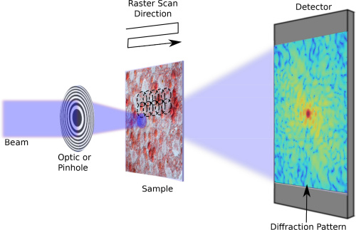
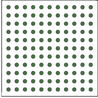
Refer to caption
(a) Ptychography set-up
Refer to caption
(b) raster scan pattern
Figure 1. Simplified ptychographic setup showing a Cartesian grid used for the overlapping raster scan positions [25].

2. Raster scan

The raster scan can be formulated as the 2D lattice with the basis {𝐯1,𝐯2}subscript𝐯1subscript𝐯2\{{\mathbf{v}}_{1},{\mathbf{v}}_{2}\}

(5) 𝒯={𝐭klk𝐯1+l𝐯2:k,l},𝐯1,𝐯22formulae-sequence𝒯conditional-setsubscript𝐭𝑘𝑙𝑘subscript𝐯1𝑙subscript𝐯2𝑘𝑙subscript𝐯1subscript𝐯2superscript2\displaystyle{\mathcal{T}}=\{\mathbf{t}_{kl}\equiv k{\mathbf{v}}_{1}+l{\mathbf{v}}_{2}:k,l\in\mathbb{Z}\},\quad{\mathbf{v}}_{1},{\mathbf{v}}_{2}\in\mathbb{Z}^{2}

acting on the object domain n2superscriptsubscript𝑛2\mathbb{Z}_{n}^{2}. Instead of 𝐯1subscript𝐯1{\mathbf{v}}_{1} and 𝐯2subscript𝐯2{\mathbf{v}}_{2} we can also take 𝐮1=11𝐯1+12𝐯2subscript𝐮1subscript11subscript𝐯1subscript12subscript𝐯2{\mathbf{u}}_{1}=\ell_{11}{\mathbf{v}}_{1}+\ell_{12}{\mathbf{v}}_{2} and 𝐮2=21𝐯1+22𝐯2subscript𝐮2subscript21subscript𝐯1subscript22subscript𝐯2{\mathbf{u}}_{2}=\ell_{21}{\mathbf{v}}_{1}+\ell_{22}{\mathbf{v}}_{2} for integers ijsubscript𝑖𝑗\ell_{ij} with 11221221=±1subscript11subscript22subscript12subscript21plus-or-minus1\ell_{11}\ell_{22}-\ell_{12}\ell_{21}=\pm 1. This ensures that 𝐯1subscript𝐯1{\mathbf{v}}_{1} and 𝐯2subscript𝐯2{\mathbf{v}}_{2} themselves are integer linear combinations of 𝐮1,𝐮2subscript𝐮1subscript𝐮2{\mathbf{u}}_{1},{\mathbf{u}}_{2}. Every lattice basis defines a fundamental parallelogram, which determines the lattice. There are five 2D lattice types, called period lattices, as given by the crystallographic restriction theorem. In contrast, there are 14 lattice types in 3D, called Bravais lattices [5].

We will focus on the simplest raster scan corresponding to the square lattice with 𝐯1=(τ,0),𝐯2=(0,τ)formulae-sequencesubscript𝐯1𝜏0subscript𝐯20𝜏{\mathbf{v}}_{1}=(\tau,0),{\mathbf{v}}_{2}=(0,\tau) of step size τ𝜏\tau\in\mathbb{N}. Our results can easily be extended to other lattice schemes.

Under the periodic boundary condition the raster scan with the step size τ=n/q,q,formulae-sequence𝜏𝑛𝑞𝑞\tau=n/q,q\in\mathbb{N}, 𝒯𝒯{\mathcal{T}} consists of 𝐭kl=τ(k,l)subscript𝐭𝑘𝑙𝜏𝑘𝑙\mathbf{t}_{kl}={\tau}(k,l), with k,l{0,1,,q1}𝑘𝑙01𝑞1k,l\in\{0,1,\cdots,q-1\}. The periodic boundary condition means that for k=q1𝑘𝑞1k=q-1 or l=q1𝑙𝑞1l=q-1 the shifted probe is wrapped around into the other end of the object domain. Denote the 𝐭klsubscript𝐭𝑘𝑙\mathbf{t}_{kl}-shifted probes and blocks by μklsuperscript𝜇𝑘𝑙\mu^{kl} and klsuperscript𝑘𝑙{\mathcal{M}}^{kl}, respectively. Likewise, denote by fklsuperscript𝑓𝑘𝑙f^{kl} the object restricted to the shifted domain klsuperscript𝑘𝑙{\mathcal{M}}^{kl}.

Depending on whether τm/2𝜏𝑚2\tau\leq m/2 (the under-shifting case) or τ>m/2𝜏𝑚2\tau>m/2 (the over-shifting case), we have two types of schemes. For the former case, all pixels of the the object participate in an equal number of diffraction patterns. For the latter case, however, 4(mτ)24superscript𝑚𝜏24(m-\tau)^{2} pixels participate in four, 4(2τm)(mτ)42𝜏𝑚𝑚𝜏4(2{\tau}-m)(m-{\tau}) pixels participate in two and (2τm)2superscript2𝜏𝑚2(2{\tau}-m)^{2} pixels participate in only one diffraction pattern, resulting in uneven coverage of the object.

2.1. The under-shifting scheme τm/2𝜏𝑚2\tau\leq m/2

For simplicity of presentation we consider the case of τ=m/p𝜏𝑚𝑝\tau=m/p for some integer p2𝑝2p\geq 2 (i.e. pn=qm𝑝𝑛𝑞𝑚pn=qm). As noted above, all pixels of the the object participate in the same number (i.e. 2p2𝑝2p) of diffraction patterns. The borderline case τ=m/2𝜏𝑚2\tau=m/2 (dubbed the minimalist scheme in [4]) corresponds to p=2𝑝2p=2.

We partition the cyclical 𝐭klsuperscript𝐭𝑘𝑙\mathbf{t}^{kl}-shifted probe μklsuperscript𝜇𝑘𝑙\mu^{kl} and the corresponding domain into equal-sized square blocks as

(6) μklsuperscript𝜇𝑘𝑙\displaystyle\mu^{kl} =\displaystyle= [μ00klμ10klμp1,0klμ01klμ11klμp1,1klμ0,p1klμ1,p1klμp1,p1kl],μijklm/p×m/pdelimited-[]matrixsubscriptsuperscript𝜇𝑘𝑙00subscriptsuperscript𝜇𝑘𝑙10subscriptsuperscript𝜇𝑘𝑙𝑝10subscriptsuperscript𝜇𝑘𝑙01subscriptsuperscript𝜇𝑘𝑙11subscriptsuperscript𝜇𝑘𝑙𝑝11subscriptsuperscript𝜇𝑘𝑙0𝑝1subscriptsuperscript𝜇𝑘𝑙1𝑝1subscriptsuperscript𝜇𝑘𝑙𝑝1𝑝1subscriptsuperscript𝜇𝑘𝑙𝑖𝑗superscript𝑚𝑝𝑚𝑝\displaystyle\left[\begin{matrix}\mu^{kl}_{00}&\mu^{kl}_{10}&\cdots&\mu^{kl}_{p-1,0}\\ \mu^{kl}_{01}&\mu^{kl}_{11}&\cdots&\mu^{kl}_{p-1,1}\\ \vdots&\vdots&\vdots&\vdots\\ \mu^{kl}_{0,p-1}&\mu^{kl}_{1,p-1}&\cdots&\mu^{kl}_{p-1,p-1}\end{matrix}\right],\quad\mu^{kl}_{ij}\in\mathbb{C}^{m/p\times m/p}
(7) klsuperscript𝑘𝑙\displaystyle{\mathcal{M}}^{kl} =\displaystyle= [00kl10klp1,0kl01kl11klp1,1kl0,p1kl1,p1klp1,p1kl],ijklm/p×m/pdelimited-[]matrixsubscriptsuperscript𝑘𝑙00subscriptsuperscript𝑘𝑙10subscriptsuperscript𝑘𝑙𝑝10subscriptsuperscript𝑘𝑙01subscriptsuperscript𝑘𝑙11subscriptsuperscript𝑘𝑙𝑝11subscriptsuperscript𝑘𝑙0𝑝1subscriptsuperscript𝑘𝑙1𝑝1subscriptsuperscript𝑘𝑙𝑝1𝑝1subscriptsuperscript𝑘𝑙𝑖𝑗superscript𝑚𝑝𝑚𝑝\displaystyle\left[\begin{matrix}{\mathcal{M}}^{kl}_{00}&{\mathcal{M}}^{kl}_{10}&\cdots&{\mathcal{M}}^{kl}_{p-1,0}\\ {\mathcal{M}}^{kl}_{01}&{\mathcal{M}}^{kl}_{11}&\cdots&{\mathcal{M}}^{kl}_{p-1,1}\\ \vdots&\vdots&\vdots&\vdots\\ {\mathcal{M}}^{kl}_{0,p-1}&{\mathcal{M}}^{kl}_{1,p-1}&\cdots&{\mathcal{M}}^{kl}_{p-1,p-1}\end{matrix}\right],\quad{\mathcal{M}}^{kl}_{ij}\in\mathbb{Z}^{m/p\times m/p}

under the periodic boundary condition

(8) μj,lq1i,k=μji1,l0k,subscriptsuperscript𝜇𝑞1𝑖𝑘𝑗𝑙subscriptsuperscript𝜇0𝑘𝑗𝑖1𝑙\displaystyle\mu^{q-1-i,k}_{j,l}=\mu^{0k}_{j-i-1,l}, μl,jk,q1i=μl,ji1k0,subscriptsuperscript𝜇𝑘𝑞1𝑖𝑙𝑗subscriptsuperscript𝜇𝑘0𝑙𝑗𝑖1\displaystyle\mu^{k,q-1-i}_{l,j}=\mu^{k0}_{l,j-i-1},
(9) j,lq1i,k=ji1,l0k,subscriptsuperscript𝑞1𝑖𝑘𝑗𝑙subscriptsuperscript0𝑘𝑗𝑖1𝑙\displaystyle{\mathcal{M}}^{q-1-i,k}_{j,l}={\mathcal{M}}^{0k}_{j-i-1,l}, l,jk,q1i=l,ji1k0subscriptsuperscript𝑘𝑞1𝑖𝑙𝑗subscriptsuperscript𝑘0𝑙𝑗𝑖1\displaystyle{\mathcal{M}}^{k,q-1-i}_{l,j}={\mathcal{M}}^{k0}_{l,j-i-1}

for all 0ij1p2,k=1,,q1,l=1,,p1.formulae-sequence0𝑖𝑗1𝑝2formulae-sequence𝑘1𝑞1𝑙1𝑝10\leq i\leq j-1\leq p-2,k=1,\dots,q-1,l=1,\dots,p-1.

Accordingly, we divide the object f𝑓f into q2superscript𝑞2q^{2} non-overlapping square blocks

(13) f=[f00fq1,0f0,q1fq1,q1],fijm/p×m/p.formulae-sequence𝑓delimited-[]subscript𝑓00subscript𝑓𝑞10subscript𝑓0𝑞1subscript𝑓𝑞1𝑞1subscript𝑓𝑖𝑗superscript𝑚𝑝𝑚𝑝\displaystyle f=\left[\begin{array}[]{ccc}f_{00}&\ldots&f_{q-1,0}\\ \vdots&\vdots&\vdots\\ f_{0,q-1}&\ldots&f_{q-1,q-1}\end{array}\right],\quad f_{ij}\in\mathbb{C}^{m/p\times m/p}.

2.2. The over-shifting scheme τ>m/2𝜏𝑚2\tau>m/2.

Because of uneven coverage of the object domain, the over-shifting case is more complicated.

We divide the shifted probe μklsuperscript𝜇𝑘𝑙\mu^{kl} and its domain as

(14) μklsuperscript𝜇𝑘𝑙\displaystyle\mu^{kl} =\displaystyle= [μ00klμ10klμ20klμ01klμ11klμ21klμ02klμ12klμ22kl]m×mdelimited-[]matrixsubscriptsuperscript𝜇𝑘𝑙00subscriptsuperscript𝜇𝑘𝑙10subscriptsuperscript𝜇𝑘𝑙20subscriptsuperscript𝜇𝑘𝑙01subscriptsuperscript𝜇𝑘𝑙11subscriptsuperscript𝜇𝑘𝑙21subscriptsuperscript𝜇𝑘𝑙02subscriptsuperscript𝜇𝑘𝑙12subscriptsuperscript𝜇𝑘𝑙22superscript𝑚𝑚\displaystyle\left[\begin{matrix}\mu^{kl}_{00}&\mu^{kl}_{10}&\mu^{kl}_{20}\\ \mu^{kl}_{01}&\mu^{kl}_{11}&\mu^{kl}_{21}\\ \mu^{kl}_{02}&\mu^{kl}_{12}&\mu^{kl}_{22}\end{matrix}\right]\in\mathbb{C}^{m\times m}
(15) klsuperscript𝑘𝑙\displaystyle{\mathcal{M}}^{kl} =\displaystyle= [00kl10kl20kl01kl11kl21kl02kl12kl22kl]m×mdelimited-[]matrixsubscriptsuperscript𝑘𝑙00subscriptsuperscript𝑘𝑙10subscriptsuperscript𝑘𝑙20subscriptsuperscript𝑘𝑙01subscriptsuperscript𝑘𝑙11subscriptsuperscript𝑘𝑙21subscriptsuperscript𝑘𝑙02subscriptsuperscript𝑘𝑙12subscriptsuperscript𝑘𝑙22superscript𝑚𝑚\displaystyle\left[\begin{matrix}{\mathcal{M}}^{kl}_{00}&{\mathcal{M}}^{kl}_{10}&{\mathcal{M}}^{kl}_{20}\\ {\mathcal{M}}^{kl}_{01}&{\mathcal{M}}^{kl}_{11}&{\mathcal{M}}^{kl}_{21}\\ {\mathcal{M}}^{kl}_{02}&{\mathcal{M}}^{kl}_{12}&{\mathcal{M}}^{kl}_{22}\end{matrix}\right]\in\mathbb{Z}^{m\times m}

under the periodic boundary condition

(16) 2jq1,k=subscriptsuperscript𝑞1𝑘2𝑗absent\displaystyle{\mathcal{M}}^{q-1,k}_{2j}= 0j0k,i2k,q1=subscriptsuperscript0𝑘0𝑗subscriptsuperscript𝑘𝑞1𝑖2absent\displaystyle{\mathcal{M}}^{0k}_{0j},\quad{\mathcal{M}}^{k,q-1}_{i2}= i0k0subscriptsuperscript𝑘0𝑖0\displaystyle{\mathcal{M}}^{k0}_{i0}
(17) μ2jq1,k=subscriptsuperscript𝜇𝑞1𝑘2𝑗absent\displaystyle\mu^{q-1,k}_{2j}= μ0j0k,μi2k,q1=subscriptsuperscript𝜇0𝑘0𝑗subscriptsuperscript𝜇𝑘𝑞1𝑖2absent\displaystyle\mu^{0k}_{0j},\quad\mu^{k,q-1}_{i2}= μi0k0,subscriptsuperscript𝜇𝑘0𝑖0\displaystyle\mu^{k0}_{i0},

for all k=1,,q1𝑘1𝑞1k=1,\dots,q-1 and i,j=0,1,2formulae-sequence𝑖𝑗012i,j=0,1,2, where q𝑞q is the number of shifts in each direction.

Note that the sizes of these blocks are not equal: the four corner blocks are (mτ)×(mτ)𝑚𝜏𝑚𝜏(m-\tau)\times(m-\tau), the center block is (2τm)×(2τm)2𝜏𝑚2𝜏𝑚(2\tau-m)\times(2\tau-m) and the rest are either (2τm)×(mτ)2𝜏𝑚𝑚𝜏(2\tau-m)\times(m-\tau) or (mτ)×(2τm)𝑚𝜏2𝜏𝑚(m-\tau)\times(2\tau-m). As a result, the corresponding partition of f𝑓f also has unequally sized blocks.

We write

(18) f=k,l=0q1fkl,fkl=[f00klf10klf20klf01klf11klf21klf02klf12klf22kl]m×mformulae-sequence𝑓superscriptsubscript𝑘𝑙0𝑞1superscript𝑓𝑘𝑙superscript𝑓𝑘𝑙delimited-[]matrixsubscriptsuperscript𝑓𝑘𝑙00subscriptsuperscript𝑓𝑘𝑙10subscriptsuperscript𝑓𝑘𝑙20subscriptsuperscript𝑓𝑘𝑙01subscriptsuperscript𝑓𝑘𝑙11subscriptsuperscript𝑓𝑘𝑙21subscriptsuperscript𝑓𝑘𝑙02subscriptsuperscript𝑓𝑘𝑙12subscriptsuperscript𝑓𝑘𝑙22superscript𝑚𝑚\displaystyle f=\bigvee_{k,l=0}^{q-1}f^{kl},\quad f^{kl}=\left[\begin{matrix}f^{kl}_{00}&f^{kl}_{10}&f^{kl}_{20}\\ f^{kl}_{01}&f^{kl}_{11}&f^{kl}_{21}\\ f^{kl}_{02}&f^{kl}_{12}&f^{kl}_{22}\end{matrix}\right]\in\mathbb{C}^{m\times m}

where, for i,j=0,1,2,k,l=0,,q1formulae-sequence𝑖𝑗012𝑘𝑙0𝑞1i,j=0,1,2,\quad k,l=0,\cdots,q-1,

f2jkl=subscriptsuperscript𝑓𝑘𝑙2𝑗absent\displaystyle f^{kl}_{2j}= f0jk+1,l,fi2k,l=subscriptsuperscript𝑓𝑘1𝑙0𝑗subscriptsuperscript𝑓𝑘𝑙𝑖2absent\displaystyle f^{k+1,l}_{0j},\quad f^{k,l}_{i2}= fi0k,l+1.subscriptsuperscript𝑓𝑘𝑙1𝑖0\displaystyle f^{k,l+1}_{i0}.

3. Affine block phases

Let S𝑆S be any cyclic subgroup of 𝒯𝒯{\mathcal{T}} generated by 𝐯𝐯{\mathbf{v}}, i.e. S:={𝐭j=j𝐯:j=0,,s1}assign𝑆conditional-setsubscript𝐭𝑗𝑗𝐯𝑗0𝑠1S:=\{\mathbf{t}_{j}=j{\mathbf{v}}:j=0,\dots,s-1\}, of order s𝑠s, i.e. s𝐯=0modn𝑠𝐯modulo0𝑛s{\mathbf{v}}=0\mod\,n. For ease of notation, denote by μk,fk,νk,gksuperscript𝜇𝑘superscript𝑓𝑘superscript𝜈𝑘superscript𝑔𝑘\mu^{k},f^{k},\nu^{k},g^{k} and Mksuperscript𝑀𝑘M^{k} for the respective 𝐭ksubscript𝐭𝑘\mathbf{t}_{k}-shifted quantities.

Theorem 3.1.

As in (4), suppose that

(19) νk(𝐧)gk(𝐧)=eiθkμk(𝐧)fk(𝐧)superscript𝜈𝑘𝐧superscript𝑔𝑘𝐧superscript𝑒isubscript𝜃𝑘superscript𝜇𝑘𝐧superscript𝑓𝑘𝐧\displaystyle\nu^{k}({\mathbf{n}})g^{k}({\mathbf{n}})=e^{{\rm i}\theta_{k}}\mu^{k}({\mathbf{n}})f^{k}({\mathbf{n}})

for all 𝐧k𝐧superscript𝑘{\mathbf{n}}\in{\mathcal{M}}^{k} and k=0,,s1𝑘0𝑠1k=0,\dots,s-1. If, for all k=0,,s1,𝑘0𝑠1k=0,\dots,s-1,

(20) kk+1supp(f)(supp(f)+𝐯),superscript𝑘superscript𝑘1supp𝑓supp𝑓𝐯\displaystyle{\mathcal{M}}^{k}\cap{\mathcal{M}}^{k+1}\cap{\hbox{\rm supp}}(f)\cap({\hbox{\rm supp}}(f)+{{\mathbf{v}}})\neq\emptyset,

then the sequence {θ0,θ1,,θs1}subscript𝜃0subscript𝜃1subscript𝜃𝑠1\{\theta_{0},\theta_{1},\dots,\theta_{s-1}\} is an arithmetic progression where Δθ=θkθk1Δ𝜃subscript𝜃𝑘subscript𝜃𝑘1\Delta\theta=\theta_{k}-\theta_{k-1} is an integer multiple of 2π/s2𝜋𝑠2\pi/s.

Remark 3.2.

If f𝑓f has a full support, i.e. supp(f)=n2supp𝑓subscriptsuperscript2𝑛{\hbox{\rm supp}}(f)=\mathbb{Z}^{2}_{n}, then (20) holds for any step size τ<m𝜏𝑚\tau<m (i.e. positive overlap).

Proof.

Rewriting (19) in the form

(21) νk+1(𝐧)gk+1(𝐧)superscript𝜈𝑘1𝐧superscript𝑔𝑘1𝐧\displaystyle\nu^{k+1}({\mathbf{n}})g^{k+1}({\mathbf{n}}) =\displaystyle= eiθk+1μk+1(𝐧)fk+1(𝐧)superscript𝑒isubscript𝜃𝑘1superscript𝜇𝑘1𝐧superscript𝑓𝑘1𝐧\displaystyle e^{{\rm i}\theta_{k+1}}\mu^{k+1}({\mathbf{n}})f^{k+1}({\mathbf{n}})

and substituting (19) into (21) for 𝐧kk+1𝐧superscript𝑘superscript𝑘1{\mathbf{n}}\in{\mathcal{M}}^{k}\cap{\mathcal{M}}^{k+1}, we have

eiθkfk(𝐧)μk(𝐧)/νk(𝐧)=eiθk+1μk+1(𝐧)/νk+1(𝐧)fk+1(𝐧)superscript𝑒isubscript𝜃𝑘superscript𝑓𝑘𝐧superscript𝜇𝑘𝐧superscript𝜈𝑘𝐧superscript𝑒isubscript𝜃𝑘1superscript𝜇𝑘1𝐧superscript𝜈𝑘1𝐧superscript𝑓𝑘1𝐧\displaystyle e^{{\rm i}\theta_{k}}f^{k}({\mathbf{n}})\mu^{k}({\mathbf{n}})/\nu^{k}({\mathbf{n}})=e^{{\rm i}\theta_{k+1}}\mu^{k+1}({\mathbf{n}})/\nu^{k+1}({\mathbf{n}})f^{k+1}({\mathbf{n}})

and hence for all 𝐧kk+1supp(f)𝐧superscript𝑘superscript𝑘1supp𝑓{\mathbf{n}}\in{\mathcal{M}}^{k}\cap{\mathcal{M}}^{k+1}\cap{\hbox{\rm supp}}(f),

(22) eiθkμk(𝐧)/νk(𝐧)=eiθk+1μk+1(𝐧)/νk+1(𝐧).superscript𝑒isubscript𝜃𝑘superscript𝜇𝑘𝐧superscript𝜈𝑘𝐧superscript𝑒isubscript𝜃𝑘1superscript𝜇𝑘1𝐧superscript𝜈𝑘1𝐧\displaystyle e^{{\rm i}\theta_{k}}\mu^{k}({\mathbf{n}})/\nu^{k}({\mathbf{n}})=e^{{\rm i}\theta_{k+1}}\mu^{k+1}({\mathbf{n}})/\nu^{k+1}({\mathbf{n}}).

For all j=0,,s1,𝑗0𝑠1j=0,\dots,s-1, substituting

(23) νj(𝐧)=νj+1(𝐧+𝐯),μj(𝐧)=μj+1(𝐧+𝐯),formulae-sequencesuperscript𝜈𝑗𝐧superscript𝜈𝑗1𝐧𝐯superscript𝜇𝑗𝐧superscript𝜇𝑗1𝐧𝐯\displaystyle\nu^{j}({\mathbf{n}})=\nu^{j+1}({\mathbf{n}}+{\mathbf{v}}),\quad\mu^{j}({\mathbf{n}})=\mu^{j+1}({\mathbf{n}}+{\mathbf{v}}),

into (22), we have that for 𝐧kk+1supp(f)𝐧superscript𝑘superscript𝑘1supp𝑓{\mathbf{n}}\in{\mathcal{M}}^{k}\cap{\mathcal{M}}^{k+1}\cap{\hbox{\rm supp}}(f)

eiθkμk+1(𝐧+𝐯)/νk+1(𝐧+𝐯)superscript𝑒isubscript𝜃𝑘superscript𝜇𝑘1𝐧𝐯superscript𝜈𝑘1𝐧𝐯\displaystyle e^{{\rm i}\theta_{k}}\mu^{k+1}({\mathbf{n}}+{\mathbf{v}})/\nu^{k+1}({\mathbf{n}}+{\mathbf{v}})
=\displaystyle= eiθk+1μk+2(𝐧+𝐯)/νk+2(𝐧+𝐯),superscript𝑒isubscript𝜃𝑘1superscript𝜇𝑘2𝐧𝐯superscript𝜈𝑘2𝐧𝐯\displaystyle e^{{\rm i}\theta_{k+1}}\mu^{k+2}({\mathbf{n}}+{\mathbf{v}})/\nu^{k+2}({\mathbf{n}}+{\mathbf{v}}),

or equivalently

(24) eiθkμk+1(𝐧)/νk+1(𝐧)superscript𝑒isubscript𝜃𝑘superscript𝜇𝑘1𝐧superscript𝜈𝑘1𝐧\displaystyle e^{{\rm i}\theta_{k}}\mu^{k+1}({\mathbf{n}})/\nu^{k+1}({\mathbf{n}}) =\displaystyle= eiθk+1μk+2(𝐧)/νk+2(𝐧),superscript𝑒isubscript𝜃𝑘1superscript𝜇𝑘2𝐧superscript𝜈𝑘2𝐧\displaystyle e^{{\rm i}\theta_{k+1}}\mu^{k+2}({\mathbf{n}})/\nu^{k+2}({\mathbf{n}}),
𝐧for-all𝐧\displaystyle\forall{\mathbf{n}} \displaystyle\in k+1k+2(supp(f)+𝐯)superscript𝑘1superscript𝑘2supp𝑓𝐯\displaystyle{\mathcal{M}}^{k+1}\cap{\mathcal{M}}^{k+2}\cap({\hbox{\rm supp}}(f)+{\mathbf{v}})

On the other hand, (22) also implies

(25) eiθk+1μk+1(𝐧)/νk+1(𝐧)superscript𝑒isubscript𝜃𝑘1superscript𝜇𝑘1𝐧superscript𝜈𝑘1𝐧\displaystyle e^{{\rm i}\theta_{k+1}}\mu^{k+1}({\mathbf{n}})/\nu^{k+1}({\mathbf{n}}) =\displaystyle= eiθk+2μk+2(𝐧)/νk+2(𝐧),superscript𝑒isubscript𝜃𝑘2superscript𝜇𝑘2𝐧superscript𝜈𝑘2𝐧\displaystyle e^{{\rm i}\theta_{k+2}}\mu^{k+2}({\mathbf{n}})/\nu^{k+2}({\mathbf{n}}),
𝐧for-all𝐧\displaystyle\forall{\mathbf{n}} \displaystyle\in k+1k+2supp(f).superscript𝑘1superscript𝑘2supp𝑓\displaystyle{\mathcal{M}}^{k+1}\cap{\mathcal{M}}^{k+2}\cap{\hbox{\rm supp}}(f).

Hence, if

kk+1supp(f)(supp(f)+𝐯)superscript𝑘superscript𝑘1supp𝑓supp𝑓𝐯\displaystyle{\mathcal{M}}^{k}\cap{\mathcal{M}}^{k+1}\cap{\hbox{\rm supp}}(f)\cap({\hbox{\rm supp}}(f)+{\mathbf{v}})\neq\emptyset

then (25) and (24) imply that

(26) eiθk+1eiθk=eiθkeiθk1,k=0,,s1formulae-sequencesuperscript𝑒isubscript𝜃𝑘1superscript𝑒isubscript𝜃𝑘superscript𝑒isubscript𝜃𝑘superscript𝑒isubscript𝜃𝑘1for-all𝑘0𝑠1\displaystyle e^{{\rm i}\theta_{k+1}}e^{-{\rm i}\theta_{k}}=e^{{\rm i}\theta_{k}}e^{-{\rm i}\theta_{k-1}},\quad\forall k=0,\dots,s-1

and hence Δθ=θkθk1Δ𝜃subscript𝜃𝑘subscript𝜃𝑘1\Delta\theta=\theta_{k}-\theta_{k-1} is independent of k𝑘k. In other words, {θ0,θ1,θ2}subscript𝜃0subscript𝜃1subscript𝜃2\{\theta_{0},\theta_{1},\theta_{2}\dots\} is an arithmetic progression.

Moreover, the periodic boundary condition and the fact that s𝐯=0mod2π𝑠𝐯modulo02𝜋s{\mathbf{v}}=0\mod 2\pi imply that sΔθ𝑠Δ𝜃s\Delta\theta is an integer multiple of 2π2𝜋2\pi. ∎

Applying Theorem 3.1 to the two-generator group 𝒯𝒯{\mathcal{T}} of the raster scan we have the following result.

Corollary 3.3.

For the full raster scan 𝒯𝒯{\mathcal{T}}, the block phases have the profile

(27) θkl=θ00+𝐫(k,l),k,l=0,,q1,formulae-sequencesubscript𝜃𝑘𝑙subscript𝜃00𝐫𝑘𝑙𝑘𝑙0𝑞1\displaystyle\theta_{kl}=\theta_{00}+\mathbf{r}\cdot(k,l),\quad k,l=0,\dots,q-1,

for some θ00subscript𝜃00\theta_{00}\in\mathbb{R} and 𝐫=(r1,r2)𝐫subscript𝑟1subscript𝑟2\mathbf{r}=(r_{1},r_{2}) where r1subscript𝑟1r_{1} and r2subscript𝑟2r_{2} are integer multiples of 2π/q2𝜋𝑞2\pi/q.

4. Raster scan ambiguities

In this section we give a complete characterization of the raster scan ambiguities other than the scaling factor and the affine phase ambiguity (1)-(2), including the arithmetically progressing phase factor inherited from the block phases and the raster grid pathology which has a τ𝜏\tau-periodic structure of τ×τ𝜏𝜏\tau\times\tau degrees of freedom. We will use the notation in Section 2.

Before we state the general result. Let us consider two simple examples to illustrate each type of ambiguity separately.

The first example shows an ambiguity resulting from the arithmetically progressing block phases which make positive and negative imprints on the object and phase estimates, respectively.

Example 4.1.

For q=3,τ=m/2formulae-sequence𝑞3𝜏𝑚2q=3,\tau=m/2, let

f𝑓\displaystyle f =\displaystyle= [f00f10f20f01f11f21f02f12f22]delimited-[]matrixsubscript𝑓00subscript𝑓10subscript𝑓20subscript𝑓01subscript𝑓11subscript𝑓21subscript𝑓02subscript𝑓12subscript𝑓22\displaystyle\left[\begin{matrix}f_{00}&f_{10}&f_{20}\\ f_{01}&f_{11}&f_{21}\\ f_{02}&f_{12}&f_{22}\end{matrix}\right]
g𝑔\displaystyle g =\displaystyle= [f00ei2π/3f10ei4π/3f20ei2π/3f01ei4π/3f11f21ei4π/3f02f12ei2π/3f22]delimited-[]matrixsubscript𝑓00superscript𝑒i2𝜋3subscript𝑓10superscript𝑒i4𝜋3subscript𝑓20superscript𝑒i2𝜋3subscript𝑓01superscript𝑒i4𝜋3subscript𝑓11subscript𝑓21superscript𝑒i4𝜋3subscript𝑓02subscript𝑓12superscript𝑒i2𝜋3subscript𝑓22\displaystyle\left[\begin{matrix}f_{00}&e^{{\rm i}2\pi/3}f_{10}&e^{{\rm i}4\pi/3}f_{20}\\ e^{{\rm i}2\pi/3}f_{01}&e^{{\rm i}4\pi/3}f_{11}&f_{21}\\ e^{{\rm i}4\pi/3}f_{02}&f_{12}&e^{{\rm i}2\pi/3}f_{22}\end{matrix}\right]

be the object and its reconstruction, respectively, where fijn/3×n/3subscript𝑓𝑖𝑗superscript𝑛3𝑛3f_{ij}\in\mathbb{C}^{n/3\times n/3}. Let

μkl=[μ00klμ10klμ01klμ11kl],νkl=[μ00klei2π/3μ10klei2π/3μ01klei4π/3μ11kl],formulae-sequencesuperscript𝜇𝑘𝑙delimited-[]matrixsubscriptsuperscript𝜇𝑘𝑙00subscriptsuperscript𝜇𝑘𝑙10subscriptsuperscript𝜇𝑘𝑙01subscriptsuperscript𝜇𝑘𝑙11superscript𝜈𝑘𝑙delimited-[]matrixsubscriptsuperscript𝜇𝑘𝑙00superscript𝑒i2𝜋3subscriptsuperscript𝜇𝑘𝑙10superscript𝑒i2𝜋3subscriptsuperscript𝜇𝑘𝑙01superscript𝑒i4𝜋3subscriptsuperscript𝜇𝑘𝑙11\displaystyle\mu^{kl}=\left[\begin{matrix}\mu^{kl}_{00}&\mu^{kl}_{10}\\ \mu^{kl}_{01}&\mu^{kl}_{11}\end{matrix}\right],\quad\nu^{kl}=\left[\begin{matrix}\mu^{kl}_{00}&e^{-{\rm i}2\pi/3}\mu^{kl}_{10}\\ e^{-{\rm i}2\pi/3}\mu^{kl}_{01}&e^{-{\rm i}4\pi/3}\mu^{kl}_{11}\end{matrix}\right],

k,l=0,1,2,formulae-sequence𝑘𝑙012k,l=0,1,2, be the (k,l)𝑘𝑙(k,l)-th shift of the probe and estimate, respectively, where μijkln/3×n/3subscriptsuperscript𝜇𝑘𝑙𝑖𝑗superscript𝑛3𝑛3\mu^{kl}_{ij}\in\mathbb{C}^{n/3\times n/3}.

Let fijsuperscript𝑓𝑖𝑗f^{ij} and gijsuperscript𝑔𝑖𝑗g^{ij} be the part of the object and estimate illuminated by μijsuperscript𝜇𝑖𝑗\mu^{ij} and νijsuperscript𝜈𝑖𝑗\nu^{ij}, respectively. It is verified easily that νijgij=ei(i+j)2π/3μijfij.direct-productsuperscript𝜈𝑖𝑗superscript𝑔𝑖𝑗direct-productsuperscript𝑒i𝑖𝑗2𝜋3superscript𝜇𝑖𝑗superscript𝑓𝑖𝑗\nu^{ij}\odot g^{ij}=e^{{\rm i}(i+j)2\pi/3}\mu^{ij}\odot f^{ij}.

The next example illustrates the periodic artifact called raster grid pathology.

Example 4.2.

For q=3,τ=m/2formulae-sequence𝑞3𝜏𝑚2q=3,\tau=m/2 and any ψn3×n3𝜓superscript𝑛3𝑛3\psi\in\mathbb{C}^{{n\over 3}\times{n\over 3}}, let

f𝑓\displaystyle f =\displaystyle= [f00f10f20f01f11f21f02f12f22]delimited-[]matrixsubscript𝑓00subscript𝑓10subscript𝑓20subscript𝑓01subscript𝑓11subscript𝑓21subscript𝑓02subscript𝑓12subscript𝑓22\displaystyle\left[\begin{matrix}f_{00}&f_{10}&f_{20}\\ f_{01}&f_{11}&f_{21}\\ f_{02}&f_{12}&f_{22}\end{matrix}\right]
g𝑔\displaystyle g =\displaystyle= [eiψf00eiψf10eiψf20eiψf01eiψf11eiψf21eiψf02eiψf12eiψf22]delimited-[]matrixdirect-productsuperscript𝑒i𝜓subscript𝑓00direct-productsuperscript𝑒i𝜓subscript𝑓10direct-productsuperscript𝑒i𝜓subscript𝑓20direct-productsuperscript𝑒i𝜓subscript𝑓01direct-productsuperscript𝑒i𝜓subscript𝑓11direct-productsuperscript𝑒i𝜓subscript𝑓21direct-productsuperscript𝑒i𝜓subscript𝑓02direct-productsuperscript𝑒i𝜓subscript𝑓12direct-productsuperscript𝑒i𝜓subscript𝑓22\displaystyle\left[\begin{matrix}e^{-{\rm i}\psi}\odot f_{00}&e^{-{\rm i}\psi}\odot f_{10}&e^{-{\rm i}\psi}\odot f_{20}\\ e^{-{\rm i}\psi}\odot f_{01}&e^{-{\rm i}\psi}\odot f_{11}&e^{-{\rm i}\psi}\odot f_{21}\\ e^{-{\rm i}\psi}\odot f_{02}&e^{-{\rm i}\psi}\odot f_{12}&e^{-{\rm i}\psi}\odot f_{22}\end{matrix}\right]

be the object and its reconstruction, respectively, where fijn/3×n/3subscript𝑓𝑖𝑗superscript𝑛3𝑛3f_{ij}\in\mathbb{C}^{n/3\times n/3}. Let

μkl=[μ00klμ10klμ01klμ11kl],νkl=[eiψμ00kleiψμ10kleiψμ01kleiψμ11kl],formulae-sequencesuperscript𝜇𝑘𝑙delimited-[]matrixsubscriptsuperscript𝜇𝑘𝑙00subscriptsuperscript𝜇𝑘𝑙10subscriptsuperscript𝜇𝑘𝑙01subscriptsuperscript𝜇𝑘𝑙11superscript𝜈𝑘𝑙delimited-[]matrixdirect-productsuperscript𝑒i𝜓subscriptsuperscript𝜇𝑘𝑙00direct-productsuperscript𝑒i𝜓subscriptsuperscript𝜇𝑘𝑙10direct-productsuperscript𝑒i𝜓subscriptsuperscript𝜇𝑘𝑙01direct-productsuperscript𝑒i𝜓subscriptsuperscript𝜇𝑘𝑙11\displaystyle\mu^{kl}=\left[\begin{matrix}\mu^{kl}_{00}&\mu^{kl}_{10}\\ \mu^{kl}_{01}&\mu^{kl}_{11}\end{matrix}\right],\quad\nu^{kl}=\left[\begin{matrix}e^{{\rm i}\psi}\odot\mu^{kl}_{00}&e^{{\rm i}\psi}\odot\mu^{kl}_{10}\\ e^{{\rm i}\psi}\odot\mu^{kl}_{01}&e^{{\rm i}\psi}\odot\mu^{kl}_{11}\end{matrix}\right],

k,l=0,1,2,formulae-sequence𝑘𝑙012k,l=0,1,2, be the (k,l)𝑘𝑙(k,l)-th shift of the probe and estimate, respectively, where μijkln/3×n/3subscriptsuperscript𝜇𝑘𝑙𝑖𝑗superscript𝑛3𝑛3\mu^{kl}_{ij}\in\mathbb{C}^{n/3\times n/3}.

Let fijsuperscript𝑓𝑖𝑗f^{ij} and gijsuperscript𝑔𝑖𝑗g^{ij} be the part of the object and estimate illuminated by μijsuperscript𝜇𝑖𝑗\mu^{ij} and νijsuperscript𝜈𝑖𝑗\nu^{ij}, respectively. It is verified easily that νijgij=μijfij.direct-productsuperscript𝜈𝑖𝑗superscript𝑔𝑖𝑗direct-productsuperscript𝜇𝑖𝑗superscript𝑓𝑖𝑗\nu^{ij}\odot g^{ij}=\mu^{ij}\odot f^{ij}.

The combination of the above two types of ambiguity gives rise to the general ambiguities for blind ptychography with the raster scan as stated next.

Theorem 4.3.

Suppose that supp(f)=n2supp𝑓superscriptsubscript𝑛2{\hbox{\rm supp}}(f)=\mathbb{Z}_{n}^{2}. Consider the raster scan 𝒯𝒯{\mathcal{T}} and suppose that an object estimate g𝑔g and a probe estimate ν00superscript𝜈00\nu^{00} satisfy the relation

(28) νklgkl=eiθklμklfkl,θkl=θ00+𝐫(k,l)formulae-sequencedirect-productsuperscript𝜈𝑘𝑙superscript𝑔𝑘𝑙direct-productsuperscript𝑒isubscript𝜃𝑘𝑙superscript𝜇𝑘𝑙superscript𝑓𝑘𝑙subscript𝜃𝑘𝑙subscript𝜃00𝐫𝑘𝑙\displaystyle\nu^{kl}\odot g^{kl}=e^{{\rm i}\theta_{kl}}\mu^{kl}\odot f^{kl},\quad\theta_{kl}=\theta_{00}+\mathbf{r}\cdot(k,l)

as given by Theorem 3.1.

Then the following statements hold.

(I). For τm/2𝜏𝑚2\tau\leq m/2, if

(29) ν0000=eiψμ0000,ψτ×τ,formulae-sequencesubscriptsuperscript𝜈0000direct-productsuperscript𝑒i𝜓subscriptsuperscript𝜇0000𝜓superscript𝜏𝜏\displaystyle\nu^{00}_{00}=e^{{\rm i}\psi}\odot\mu^{00}_{00},\quad\psi\in\mathbb{C}^{\tau\times\tau},

then

(30) νkl00subscriptsuperscript𝜈00𝑘𝑙\displaystyle\nu^{00}_{kl} =\displaystyle= ei𝐫(k,l)eiψμkl00,k,l=0,,p1formulae-sequencedirect-productsuperscript𝑒i𝐫𝑘𝑙superscript𝑒i𝜓subscriptsuperscript𝜇00𝑘𝑙𝑘𝑙0𝑝1\displaystyle e^{-{\rm i}\mathbf{r}\cdot(k,l)}e^{{\rm i}\psi}\odot\mu^{00}_{kl},\quad k,l=0,\dots,p-1
(31) gklsubscript𝑔𝑘𝑙\displaystyle g_{kl} =\displaystyle= eiθ00ei𝐫(k,l)eiψfkl,k,l=0,,q1.formulae-sequencedirect-productsuperscript𝑒isubscript𝜃00superscript𝑒i𝐫𝑘𝑙superscript𝑒i𝜓subscript𝑓𝑘𝑙𝑘𝑙0𝑞1\displaystyle e^{{\rm i}\theta_{00}}e^{{\rm i}\mathbf{r}\cdot(k,l)}e^{-{\rm i}\psi}\odot f_{kl},\quad k,l=0,\dots,q-1.

(II). For τ>m/2𝜏𝑚2\tau>m/2, if

(32) [ν0000ν1000ν0100ν1100]=eiψ[μ0000μ1000μ0100μ1100]delimited-[]matrixsubscriptsuperscript𝜈0000subscriptsuperscript𝜈0010subscriptsuperscript𝜈0001subscriptsuperscript𝜈0011direct-productsuperscript𝑒i𝜓delimited-[]matrixsubscriptsuperscript𝜇0000subscriptsuperscript𝜇0010subscriptsuperscript𝜇0001subscriptsuperscript𝜇0011\displaystyle\left[\begin{matrix}\nu^{00}_{00}&\nu^{00}_{10}\\ \nu^{00}_{01}&\nu^{00}_{11}\end{matrix}\right]=e^{{\rm i}\psi}\odot\left[\begin{matrix}\mu^{00}_{00}&\mu^{00}_{10}\\ \mu^{00}_{01}&\mu^{00}_{11}\\ \end{matrix}\right]

for some

ψ=[ψ00ψ10ψ01ψ11]τ×τ,𝜓delimited-[]matrixsubscript𝜓00subscript𝜓10subscript𝜓01subscript𝜓11superscript𝜏𝜏\psi=\left[\begin{matrix}\psi_{00}&\psi_{10}\\ \psi_{01}&\psi_{11}\end{matrix}\right]\in\mathbb{C}^{\tau\times\tau},

then

(33) [g00klg10klg01klg11kl]=eiθ00ei𝐫(k,l)eiψ[f00klf10klf01klf11kl]delimited-[]matrixsubscriptsuperscript𝑔𝑘𝑙00subscriptsuperscript𝑔𝑘𝑙10subscriptsuperscript𝑔𝑘𝑙01subscriptsuperscript𝑔𝑘𝑙11direct-productsuperscript𝑒isubscript𝜃00superscript𝑒i𝐫𝑘𝑙superscript𝑒i𝜓delimited-[]matrixsubscriptsuperscript𝑓𝑘𝑙00subscriptsuperscript𝑓𝑘𝑙10subscriptsuperscript𝑓𝑘𝑙01subscriptsuperscript𝑓𝑘𝑙11\displaystyle\left[\begin{matrix}g^{kl}_{00}&g^{kl}_{10}\\ g^{kl}_{01}&g^{kl}_{11}\end{matrix}\right]=e^{{\rm i}\theta_{00}}e^{{\rm i}\mathbf{r}\cdot(k,l)}e^{-{\rm i}\psi}\odot\left[\begin{matrix}f^{kl}_{00}&f^{kl}_{10}\\ f^{kl}_{01}&f^{kl}_{11}\end{matrix}\right]

for all k,l=0,,q1formulae-sequence𝑘𝑙0𝑞1k,l=0,\dots,q-1. Moreover,

(34) ν2j00subscriptsuperscript𝜈002𝑗\displaystyle\nu^{00}_{2j} =\displaystyle= eir1eiψ0jμ2j00,j=0,1formulae-sequencedirect-productsuperscript𝑒isubscript𝑟1superscript𝑒isubscript𝜓0𝑗subscriptsuperscript𝜇002𝑗𝑗01\displaystyle e^{-{\rm i}r_{1}}e^{{\rm i}\psi_{0j}}\odot\mu^{00}_{2j},\quad j=0,1
(35) νj200subscriptsuperscript𝜈00𝑗2\displaystyle\nu^{00}_{j2} =\displaystyle= eir2eiψj0μj200,j=0,1formulae-sequencedirect-productsuperscript𝑒isubscript𝑟2superscript𝑒isubscript𝜓𝑗0subscriptsuperscript𝜇00𝑗2𝑗01\displaystyle e^{-{\rm i}r_{2}}e^{{\rm i}\psi_{j0}}\odot\mu^{00}_{j2},\quad j=0,1
(36) ν2200subscriptsuperscript𝜈0022\displaystyle\nu^{00}_{22} =\displaystyle= ei(r1+r2)eiψ00μ2200direct-productsuperscript𝑒isubscript𝑟1subscript𝑟2superscript𝑒isubscript𝜓00subscriptsuperscript𝜇0022\displaystyle e^{-{\rm i}(r_{1}+r_{2})}e^{{\rm i}\psi_{00}}\odot\mu^{00}_{22}

and hence

(37) g2jklsubscriptsuperscript𝑔𝑘𝑙2𝑗\displaystyle g^{kl}_{2j} =\displaystyle= eiθ00ei𝐫(k+1,l)eiψ0jf2jkl,j=0,1formulae-sequencedirect-productsuperscript𝑒isubscript𝜃00superscript𝑒i𝐫𝑘1𝑙superscript𝑒isubscript𝜓0𝑗subscriptsuperscript𝑓𝑘𝑙2𝑗𝑗01\displaystyle e^{{\rm i}\theta_{00}}e^{{\rm i}\mathbf{r}\cdot({k+1,l})}e^{-{\rm i}\psi_{0j}}\odot f^{kl}_{2j},\quad j=0,1
(38) gj2klsubscriptsuperscript𝑔𝑘𝑙𝑗2\displaystyle g^{kl}_{j2} =\displaystyle= eiθ00ei𝐫(k,l+1)eiψj0fj2kl,j=0,1formulae-sequencedirect-productsuperscript𝑒isubscript𝜃00superscript𝑒i𝐫𝑘𝑙1superscript𝑒isubscript𝜓𝑗0subscriptsuperscript𝑓𝑘𝑙𝑗2𝑗01\displaystyle e^{{\rm i}\theta_{00}}e^{{\rm i}\mathbf{r}\cdot({k,l+1})}e^{-{\rm i}\psi_{j0}}\odot f^{kl}_{j2},\quad j=0,1
(39) g22klsubscriptsuperscript𝑔𝑘𝑙22\displaystyle g^{kl}_{22} =\displaystyle= eiθ00ei𝐫(k+1,l+1)eiψ00f22kl.direct-productsuperscript𝑒isubscript𝜃00superscript𝑒i𝐫𝑘1𝑙1superscript𝑒isubscript𝜓00subscriptsuperscript𝑓𝑘𝑙22\displaystyle e^{{\rm i}\theta_{00}}e^{{\rm i}\mathbf{r}\cdot({k+1,l+1})}e^{-{\rm i}\psi_{00}}\odot f^{kl}_{22}.
Remark 4.4.

Since ψ𝜓\psi is any complex τ×τ𝜏𝜏\tau\times\tau matrix, (29) and (32) represent the maximum degrees of ambiguity over the respective initial sub-blocks. This ambiguity is transmitted to other sub-blocks, forming periodic artifacts called the raster grid pathology.

On top of the periodic artifacts, there is the non-periodic ambiguity inherited from the affine block phase profile. The non-periodic arithmetically progressing ambiguity is different from the affine phase ambiguity (1)-(2) as they manifest on different scales: the former on the block scale while the latter on the pixel scale.

Proof.

(I). For τm/2𝜏𝑚2\tau\leq m/2, recall the decomposition

νklsuperscript𝜈𝑘𝑙\displaystyle\nu^{kl} =\displaystyle= [ν00klν10klνp1,0klν01klμ11klνp1,1klν0,p1klν1,p1klνp1,p1kl],g=[g00gq1,0g0,q1gq1,q1],delimited-[]matrixsubscriptsuperscript𝜈𝑘𝑙00subscriptsuperscript𝜈𝑘𝑙10subscriptsuperscript𝜈𝑘𝑙𝑝10subscriptsuperscript𝜈𝑘𝑙01subscriptsuperscript𝜇𝑘𝑙11subscriptsuperscript𝜈𝑘𝑙𝑝11subscriptsuperscript𝜈𝑘𝑙0𝑝1subscriptsuperscript𝜈𝑘𝑙1𝑝1subscriptsuperscript𝜈𝑘𝑙𝑝1𝑝1𝑔delimited-[]subscript𝑔00subscript𝑔𝑞10subscript𝑔0𝑞1subscript𝑔𝑞1𝑞1\displaystyle\left[\begin{matrix}\nu^{kl}_{00}&\nu^{kl}_{10}&\cdots&\nu^{kl}_{p-1,0}\\ \nu^{kl}_{01}&\mu^{kl}_{11}&\cdots&\nu^{kl}_{p-1,1}\\ \vdots&\vdots&\vdots&\vdots\\ \nu^{kl}_{0,p-1}&\nu^{kl}_{1,p-1}&\cdots&\nu^{kl}_{p-1,p-1}\end{matrix}\right],\quad g=\left[\begin{array}[]{ccc}g_{00}&\ldots&g_{q-1,0}\\ \vdots&\vdots&\vdots\\ g_{0,q-1}&\ldots&g_{q-1,q-1}\end{array}\right],

with νijkl,gijm/p×m/psubscriptsuperscript𝜈𝑘𝑙𝑖𝑗subscript𝑔𝑖𝑗superscript𝑚𝑝𝑚𝑝\nu^{kl}_{ij},g_{ij}\in\mathbb{C}^{m/p\times m/p}, in analogy to (6) and (13).

g00=eiθ00eiψf00subscript𝑔00direct-productsuperscript𝑒isubscript𝜃00superscript𝑒i𝜓subscript𝑓00g_{00}=e^{{\rm i}\theta_{00}}e^{-{\rm i}\psi}\odot f_{00}

by restricting (28) to 0000subscriptsuperscript0000{\mathcal{M}}^{00}_{00}.

For 𝐧0010𝐧superscriptsubscript0010{\mathbf{n}}\in{\mathcal{M}}_{00}^{10}, we have

ν0010g10=eiθ10μ0010f10,direct-productsuperscriptsubscript𝜈0010subscript𝑔10direct-productsuperscript𝑒isubscript𝜃10subscriptsuperscript𝜇1000subscript𝑓10\displaystyle\nu_{00}^{10}\odot g_{10}=e^{{\rm i}\theta_{10}}\mu^{10}_{00}\odot f_{10},

by (28), and

ν0010(𝐧)=ν0000(𝐧(τ,0))=(eiψμ0000)(𝐧(τ,0))=(eiψμ0010)(𝐧)superscriptsubscript𝜈0010𝐧subscriptsuperscript𝜈0000𝐧𝜏0direct-productsuperscript𝑒i𝜓superscriptsubscript𝜇0000𝐧𝜏0direct-productsuperscript𝑒i𝜓subscriptsuperscript𝜇1000𝐧\nu_{00}^{10}({\mathbf{n}})=\nu^{00}_{00}({\mathbf{n}}-(\tau,0))=(e^{{\rm i}\psi}\odot\mu_{00}^{00})({\mathbf{n}}-(\tau,0))=(e^{{\rm i}\psi}\odot\mu^{10}_{00})({\mathbf{n}})

by (29). Hence

g10=eiθ10eiψf10subscript𝑔10direct-productsuperscript𝑒isubscript𝜃10superscript𝑒i𝜓subscript𝑓10g_{10}=e^{{\rm i}\theta_{10}}e^{-{\rm i}\psi}\odot f_{10}

implying

ν1000g10=eiθ10eiψν1000f10=eiθ00μ1000f10direct-productsubscriptsuperscript𝜈0010subscript𝑔10direct-productsuperscript𝑒isubscript𝜃10superscript𝑒i𝜓subscriptsuperscript𝜈0010subscript𝑓10direct-productsuperscript𝑒isubscript𝜃00subscriptsuperscript𝜇0010subscript𝑓10\nu^{00}_{10}\odot g_{10}=e^{{\rm i}\theta_{10}}e^{-{\rm i}\psi}\nu^{00}_{10}\odot f_{10}=e^{{\rm i}\theta_{00}}\mu^{00}_{10}\odot f_{10}

by (28) and consequently

ν1000=eiθ00eiθ10eiψμ1000.superscriptsubscript𝜈1000superscript𝑒isubscript𝜃00superscript𝑒isubscript𝜃10superscript𝑒i𝜓subscriptsuperscript𝜇0010\nu_{10}^{00}=e^{{\rm i}\theta_{00}}e^{-{\rm i}\theta_{10}}e^{{\rm i}\psi}\mu^{00}_{10}.

Repeating the same argument for the adjacent blocks in both directions, we obtain

νkl00subscriptsuperscript𝜈00𝑘𝑙\displaystyle\nu^{00}_{kl} =\displaystyle= eiθ00eiθkleiψμkl00direct-productsuperscript𝑒isubscript𝜃00superscript𝑒isubscript𝜃𝑘𝑙superscript𝑒i𝜓subscriptsuperscript𝜇00𝑘𝑙\displaystyle e^{{\rm i}\theta_{00}}e^{-{\rm i}\theta_{kl}}e^{{\rm i}\psi}\odot\mu^{00}_{kl}
gklsubscript𝑔𝑘𝑙\displaystyle g_{kl} =\displaystyle= eiθkleiψfkldirect-productsuperscript𝑒isubscript𝜃𝑘𝑙superscript𝑒i𝜓subscript𝑓𝑘𝑙\displaystyle e^{{\rm i}\theta_{kl}}e^{-{\rm i}\psi}\odot f_{kl}

which are equivalent to (30) and (31) in view of the block phase profile in (27).

(II). First recall

μklsuperscript𝜇𝑘𝑙\displaystyle\mu^{kl} =\displaystyle= [μ00klμ10klμ20klμ01klμ11klμ21klμ02klμ12klμ22kl],g=k,l=0q1gkl,gkl=[g00klg10klg20klg01klg11klg21klg02klg12klg22kl]formulae-sequencedelimited-[]matrixsubscriptsuperscript𝜇𝑘𝑙00subscriptsuperscript𝜇𝑘𝑙10subscriptsuperscript𝜇𝑘𝑙20subscriptsuperscript𝜇𝑘𝑙01subscriptsuperscript𝜇𝑘𝑙11subscriptsuperscript𝜇𝑘𝑙21subscriptsuperscript𝜇𝑘𝑙02subscriptsuperscript𝜇𝑘𝑙12subscriptsuperscript𝜇𝑘𝑙22𝑔superscriptsubscript𝑘𝑙0𝑞1superscript𝑔𝑘𝑙superscript𝑔𝑘𝑙delimited-[]matrixsubscriptsuperscript𝑔𝑘𝑙00subscriptsuperscript𝑔𝑘𝑙10subscriptsuperscript𝑔𝑘𝑙20subscriptsuperscript𝑔𝑘𝑙01subscriptsuperscript𝑔𝑘𝑙11subscriptsuperscript𝑔𝑘𝑙21subscriptsuperscript𝑔𝑘𝑙02subscriptsuperscript𝑔𝑘𝑙12subscriptsuperscript𝑔𝑘𝑙22\displaystyle\left[\begin{matrix}\mu^{kl}_{00}&\mu^{kl}_{10}&\mu^{kl}_{20}\\ \mu^{kl}_{01}&\mu^{kl}_{11}&\mu^{kl}_{21}\\ \mu^{kl}_{02}&\mu^{kl}_{12}&\mu^{kl}_{22}\end{matrix}\right],\quad g=\bigvee_{k,l=0}^{q-1}g^{kl},\quad g^{kl}=\left[\begin{matrix}g^{kl}_{00}&g^{kl}_{10}&g^{kl}_{20}\\ g^{kl}_{01}&g^{kl}_{11}&g^{kl}_{21}\\ g^{kl}_{02}&g^{kl}_{12}&g^{kl}_{22}\end{matrix}\right]

in analogy to (14) and (18).

Since

(41) νkl(𝐧)=ν00(𝐧τ(k,l))),μkl(𝐧)=μ00(𝐧τ(k,l)),\displaystyle\nu^{kl}({\mathbf{n}})=\nu^{00}({\mathbf{n}}-\tau(k,l))),\quad\mu^{kl}({\mathbf{n}})=\mu^{00}({\mathbf{n}}-\tau(k,l)),

(33) follows from (32) and (28).

By (32) and restricting (28) to 0j10,j=0,1,formulae-sequencesubscriptsuperscript100𝑗𝑗01{\mathcal{M}}^{10}_{0j},j=0,1, we obtain

g2j00=g0j10=eiθ10eiψ0jf0j10=eiθ10eiψ0jf2j00,j=0,1,formulae-sequencesubscriptsuperscript𝑔002𝑗subscriptsuperscript𝑔100𝑗direct-productsuperscript𝑒isubscript𝜃10superscript𝑒isubscript𝜓0𝑗subscriptsuperscript𝑓100𝑗direct-productsuperscript𝑒isubscript𝜃10superscript𝑒isubscript𝜓0𝑗subscriptsuperscript𝑓002𝑗𝑗01g^{00}_{2j}=g^{10}_{0j}=e^{{\rm i}\theta_{10}}e^{-{\rm i}\psi_{0j}}\odot f^{10}_{0j}=e^{{\rm i}\theta_{10}}e^{-{\rm i}\psi_{0j}}\odot f^{00}_{2j},\quad j=0,1,

which implies by (28)

ν2j00subscriptsuperscript𝜈002𝑗\displaystyle\nu^{00}_{2j} =\displaystyle= eiθ00eiθ10eiψ0jμ2j00,j=0,1,formulae-sequencedirect-productsuperscript𝑒isubscript𝜃00superscript𝑒isubscript𝜃10superscript𝑒isubscript𝜓0𝑗subscriptsuperscript𝜇002𝑗𝑗01\displaystyle e^{{\rm i}\theta_{00}}e^{-{\rm i}\theta_{10}}e^{{\rm i}\psi_{0j}}\odot\mu^{00}_{2j},\quad j=0,1,
νj200subscriptsuperscript𝜈00𝑗2\displaystyle\nu^{00}_{j2} =\displaystyle= eiθ00eiθ01eiψj0μj200,j=0,1,formulae-sequencedirect-productsuperscript𝑒isubscript𝜃00superscript𝑒isubscript𝜃01superscript𝑒isubscript𝜓𝑗0subscriptsuperscript𝜇00𝑗2𝑗01\displaystyle e^{{\rm i}\theta_{00}}e^{-{\rm i}\theta_{01}}e^{{\rm i}\psi_{j0}}\odot\mu^{00}_{j2},\quad j=0,1,

and consequently (34) and (35).

By (41) and restricting (28) to 2jkl,j2kl,j=0,1,formulae-sequencesubscriptsuperscript𝑘𝑙2𝑗subscriptsuperscript𝑘𝑙𝑗2𝑗01{\mathcal{M}}^{kl}_{2j},{\mathcal{M}}^{kl}_{j2},j=0,1, we have (37) and (38).

For (39) with (k,l)=(0,0)𝑘𝑙00(k,l)=(0,0), the block 0210=2200subscriptsuperscript1002subscriptsuperscript0022{\mathcal{M}}^{10}_{02}={\mathcal{M}}^{00}_{22} is masked by μ0210subscriptsuperscript𝜇1002\mu^{10}_{02}, a translate of μ0200subscriptsuperscript𝜇0002\mu^{00}_{02}. By restricting (28) to 0210subscriptsuperscript1002{\mathcal{M}}^{10}_{02},

(42) g2200=g0210=ei(θ10+θ01θ00)eiψ00f2200.subscriptsuperscript𝑔0022subscriptsuperscript𝑔1002direct-productsuperscript𝑒isubscript𝜃10subscript𝜃01subscript𝜃00superscript𝑒isubscript𝜓00subscriptsuperscript𝑓0022\displaystyle g^{00}_{22}=g^{10}_{02}=e^{{\rm i}(\theta_{10}+\theta_{01}-\theta_{00})}e^{-{\rm i}\psi_{00}}\odot f^{00}_{22}.

which is equivalent to (39) with (k,l)=(0,0)𝑘𝑙00(k,l)=(0,0). Then (28) and (42) imply

(43) ν2200=ei(θ00θ10)ei(θ00θ01)eiψ00μ2200subscriptsuperscript𝜈0022direct-productsuperscript𝑒isubscript𝜃00subscript𝜃10superscript𝑒isubscript𝜃00subscript𝜃01superscript𝑒isubscript𝜓00subscriptsuperscript𝜇0022\displaystyle\nu^{00}_{22}=e^{{\rm i}(\theta_{00}-\theta_{10})}e^{{\rm i}(\theta_{00}-\theta_{01})}e^{{\rm i}\psi_{00}}\odot\mu^{00}_{22}

which is equivalent to (36).

For (39) with general k,l𝑘𝑙k,l, by restricting (28) to 22klsubscriptsuperscript𝑘𝑙22{\mathcal{M}}^{kl}_{22} and (43) we have

g22kl=eiθklei(θ10θ00)ei(θ01θ00)eiψ00f00klsubscriptsuperscript𝑔𝑘𝑙22direct-productsuperscript𝑒isubscript𝜃𝑘𝑙superscript𝑒isubscript𝜃10subscript𝜃00superscript𝑒isubscript𝜃01subscript𝜃00superscript𝑒isubscript𝜓00subscriptsuperscript𝑓𝑘𝑙00g^{kl}_{22}=e^{{\rm i}\theta_{kl}}e^{{\rm i}(\theta_{10}-\theta_{00})}e^{{\rm i}(\theta_{01}-\theta_{00})}e^{-{\rm i}\psi_{00}}\odot f^{kl}_{00}

and hence (39). ∎

When τ=1𝜏1\tau=1, the non-periodic, arithmetically progressing ambiguity and the affine phase ambiguity become the same. In addition, for τ=1𝜏1\tau=1 the raster grid pathology becomes a constant phase factor which can be ignored [18].

Corollary 4.5.

If τ=1𝜏1\tau=1 (i.e. q=n,p=mformulae-sequence𝑞𝑛𝑝𝑚q=n,p=m) and (28) holds, then the probe and the object can be uniquely and simultaneously determined.

Proof.

For τ=1𝜏1\tau=1, μ00subscript𝜇00\mu_{00} consists of just one pixel and ψ𝜓\psi is a number. Hence μ00=ν00superscript𝜇00superscript𝜈00\mu^{00}=\nu^{00} up to a constant phase factor and (30)-(31) then imply that the affine phase ambiguity is the only ambiguity modulo the constant phase factor.

5. Slightly perturbed raster scan

Refer to caption
(a) Perturbed grid (44)
Refer to caption
(b) Perturbed grid (45)

In this section, we demonstrate a simple way for removing all the raster scan ambiguities except for the scaling factor and the affine phase ambiguity.

For the rest of the paper, we assume that f𝑓f does not vanish in n2superscriptsubscript𝑛2\mathbb{Z}_{n}^{2}.

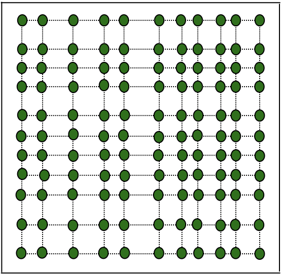
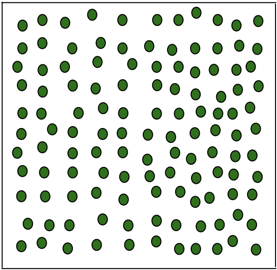
We consider the perturbed raster scan (Fig. 2(b)(a))

(44) 𝐭kl=τ(k,l)+(δk1,δl2),k,l=0,,q1formulae-sequencesubscript𝐭𝑘𝑙𝜏𝑘𝑙subscriptsuperscript𝛿1𝑘subscriptsuperscript𝛿2𝑙𝑘𝑙0𝑞1\displaystyle\mathbf{t}_{kl}=\tau(k,l)+(\delta^{1}_{k},\delta^{2}_{l}),\quad k,l=0,\dots,q-1

where δk1,δl2subscriptsuperscript𝛿1𝑘subscriptsuperscript𝛿2𝑙\delta^{1}_{k},\delta^{2}_{l} are small integers relative to τ𝜏\tau and mτ𝑚𝜏m-\tau (see Theorem 5.5 for details). More general than (44) is the perturbed grid pattern (Fig. 2(b)(b)):

(45) 𝐭kl=τ(k,l)+(δkl1,δkl2),k,l=0,,q1,formulae-sequencesubscript𝐭𝑘𝑙𝜏𝑘𝑙subscriptsuperscript𝛿1𝑘𝑙subscriptsuperscript𝛿2𝑘𝑙𝑘𝑙0𝑞1\displaystyle\mathbf{t}_{kl}=\tau(k,l)+(\delta^{1}_{kl},\delta^{2}_{kl}),\quad k,l=0,\dots,q-1,

which is harder to analyze and implement in experimental practice (we will only present numerical simulation for it). Without loss of generality we set δ01=δ02=0subscriptsuperscript𝛿10superscriptsubscript𝛿020\delta^{1}_{0}=\delta_{0}^{2}=0 and hence 𝐭00=(0,0)subscript𝐭0000\mathbf{t}_{00}=(0,0).

Let us express the probe and object errors in terms of

(46) ν00(𝐧)/μ00(𝐧)superscript𝜈00𝐧superscript𝜇00𝐧\displaystyle\nu^{00}({\mathbf{n}})/\mu^{00}({\mathbf{n}}) :=assign\displaystyle:= α(𝐧)exp(iϕ(𝐧)),𝐧00𝛼𝐧iitalic-ϕ𝐧𝐧superscript00\displaystyle\alpha({\mathbf{n}})\exp{({\rm i}\phi({\mathbf{n}}))},\quad{\mathbf{n}}\in{\mathcal{M}}^{00}
(47) h(𝐧)𝐧\displaystyle h({\mathbf{n}}) :=assign\displaystyle:= lng(𝐧)lnf(𝐧),𝐧n2,𝑔𝐧𝑓𝐧𝐧superscriptsubscript𝑛2\displaystyle\ln g({\mathbf{n}})-\ln f({\mathbf{n}}),\quad{\mathbf{n}}\in\mathbb{Z}_{n}^{2},

where we assume α(𝐧)0𝛼𝐧0\alpha({\mathbf{n}})\neq 0 for all 𝐧00𝐧superscript00{\mathbf{n}}\in{\mathcal{M}}^{00}, and rewrite (4) as

(48) h(𝐧+𝐭)𝐧𝐭\displaystyle h({\mathbf{n}}+\mathbf{t}) =\displaystyle= iθ𝐭lnα(𝐧)iϕ(𝐧)modi2π,moduloisubscript𝜃𝐭𝛼𝐧iitalic-ϕ𝐧i2𝜋\displaystyle{\rm i}\theta_{\mathbf{t}}-\ln\alpha({\mathbf{n}})-{\rm i}\phi({\mathbf{n}})\mod{\rm i}2\pi,

for 𝐧00𝐧superscript00{\mathbf{n}}\in{\mathcal{M}}^{00}.

By (48) with 𝐭=(0,0)𝐭00\mathbf{t}=(0,0),

(49) h(𝐧)=iθ00lnα(𝐧)iϕ(𝐧),𝐧00formulae-sequence𝐧isubscript𝜃00𝛼𝐧iitalic-ϕ𝐧for-all𝐧superscript00\displaystyle h({\mathbf{n}})={\rm i}\theta_{00}-\ln\alpha({\mathbf{n}})-{\rm i}\phi({\mathbf{n}}),\quad\forall{\mathbf{n}}\in{\mathcal{M}}^{00}

and hence for all 𝐭𝒯𝐭𝒯\mathbf{t}\in{\mathcal{T}} and 𝐧00𝐧superscript00{\mathbf{n}}\in{\mathcal{M}}^{00}

(50) h(𝐧+𝐭)h(𝐧)=iθ𝐭iθ00modi2π.𝐧𝐭𝐧moduloisubscript𝜃𝐭isubscript𝜃00i2𝜋\displaystyle h({\mathbf{n}}+\mathbf{t})-h({\mathbf{n}})={\rm i}\theta_{\mathbf{t}}-{\rm i}\theta_{00}\mod{\rm i}2\pi.

We wish to generalize such a relationship to the case where 𝐭𝐭\mathbf{t} in (64) is replaced by 𝐞1=(1,0)subscript𝐞110\mathbf{e}_{1}=(1,0) and 𝐞2=(0,1)subscript𝐞201\mathbf{e}_{2}=(0,1).

5.1. A simple perturbation

Let us first study the simple example of the two-shift perturbation to the raster-scan with δ21=δ22=1subscriptsuperscript𝛿12subscriptsuperscript𝛿221\delta^{1}_{2}=\delta^{2}_{2}=-1 but all other δkj=0subscriptsuperscript𝛿𝑗𝑘0\delta^{j}_{k}=0, i.e. 𝐭kl=τ(k,l)subscript𝐭𝑘𝑙𝜏𝑘𝑙\mathbf{t}_{kl}=\tau(k,l) for (k,l)(2,0),(0,2)𝑘𝑙2002(k,l)\neq(2,0),(0,2). Then

(51) h(𝐧+2𝐭10𝐭20)=h(𝐧+(1,0))𝐧2subscript𝐭10subscript𝐭20𝐧10\displaystyle h({\mathbf{n}}+2\mathbf{t}_{10}-\mathbf{t}_{20})=h({\mathbf{n}}+(1,0))
(52) h(𝐧+2𝐭01𝐭02)=h(𝐧+(0,1)).𝐧2subscript𝐭01subscript𝐭02𝐧01\displaystyle h({\mathbf{n}}+2\mathbf{t}_{01}-\mathbf{t}_{02})=h({\mathbf{n}}+(0,1)).

There are several routes of reduction from (1,0)10(1,0) to (0,0)00(0,0) via the shifts in 𝒯𝒯{\mathcal{T}}. For example, we can proceed from (1,0)=2𝐭10𝐭20102subscript𝐭10subscript𝐭20(1,0)=2\mathbf{t}_{10}-\mathbf{t}_{20} to (0,0)00(0,0) along the path

(53) (2𝐭10𝐭20)(𝐭10𝐭20)𝐭10(0,0)2subscript𝐭10subscript𝐭20subscript𝐭10subscript𝐭20subscript𝐭1000\displaystyle(2\mathbf{t}_{10}-\mathbf{t}_{20})\longrightarrow(\mathbf{t}_{10}-\mathbf{t}_{20})\longrightarrow\mathbf{t}_{10}\longrightarrow(0,0)

by repeatedly applying (50) where the direction of the second step is to be reversed since 𝐭20𝒯subscript𝐭20𝒯-\mathbf{t}_{20}\not\in{\mathcal{T}} (𝒯𝒯{\mathcal{T}} is no longer a group even under the periodic boundary condition). The direction is important for keeping track of the domain of validity of (50) along the path. Hence for all

(54) 𝐧(00+𝐭20𝐭10)00𝐧superscript00subscript𝐭20subscript𝐭10superscript00\displaystyle{\mathbf{n}}\in({\mathcal{M}}^{00}+\mathbf{t}_{20}-\mathbf{t}_{10})\cap{\mathcal{M}}^{00}

we have

h(𝐧+2𝐭10𝐭20)𝐧2subscript𝐭10subscript𝐭20\displaystyle h({\mathbf{n}}+2\mathbf{t}_{10}-\mathbf{t}_{20}) =\displaystyle= h(𝐧+𝐭10𝐭20)+iθ10iθ00𝐧subscript𝐭10subscript𝐭20isubscript𝜃10isubscript𝜃00\displaystyle h({\mathbf{n}}+\mathbf{t}_{10}-\mathbf{t}_{20})+{\rm i}\theta_{10}-{\rm i}\theta_{00}
=\displaystyle= h(𝐧+𝐭10)+iθ10iθ20𝐧subscript𝐭10isubscript𝜃10isubscript𝜃20\displaystyle h({\mathbf{n}}+\mathbf{t}_{10})+{\rm i}\theta_{10}-{\rm i}\theta_{20}
=\displaystyle= h(𝐧)+2iθ10iθ20iθ00𝐧2isubscript𝜃10isubscript𝜃20isubscript𝜃00\displaystyle h({\mathbf{n}})+2{\rm i}\theta_{10}-{\rm i}\theta_{20}-{\rm i}\theta_{00}

and hence

(55) h(𝐧+(1,0))=h(𝐧)+iΔ1,Δ1:=2θ10θ20θ00formulae-sequence𝐧10𝐧isuperscriptΔ1assignsuperscriptΔ12subscript𝜃10subscript𝜃20subscript𝜃00\displaystyle h({\mathbf{n}}+(1,0))=h({\mathbf{n}})+{\rm i}\Delta^{1},\quad\Delta^{1}:=2\theta_{10}-\theta_{20}-\theta_{00}

modulo i2πi2𝜋{\rm i}2\pi.

Let us consider another alternative route for reduction:

(56) (2𝐭10𝐭20)2𝐭10𝐭10(0,0)2subscript𝐭10subscript𝐭202subscript𝐭10subscript𝐭1000\displaystyle(2\mathbf{t}_{10}-\mathbf{t}_{20})\longrightarrow 2\mathbf{t}_{10}\longrightarrow\mathbf{t}_{10}\longrightarrow(0,0)

where the proper direction for the first step in applying (50) is reversed. Keeping track of the domain of validity along the path, we have

h(𝐧+2𝐭10𝐭20)𝐧2subscript𝐭10subscript𝐭20\displaystyle h({\mathbf{n}}+2\mathbf{t}_{10}-\mathbf{t}_{20}) =\displaystyle= h(𝐧+2𝐭10)iθ20+iθ00𝐧2subscript𝐭10isubscript𝜃20isubscript𝜃00\displaystyle h({\mathbf{n}}+2\mathbf{t}_{10})-{\rm i}\theta_{20}+{\rm i}\theta_{00}
=\displaystyle= h(𝐧+𝐭10)+iθ10iθ20𝐧subscript𝐭10isubscript𝜃10isubscript𝜃20\displaystyle h({\mathbf{n}}+\mathbf{t}_{10})+{\rm i}\theta_{10}-{\rm i}\theta_{20}
=\displaystyle= h(𝐧)+iΔ1𝐧isuperscriptΔ1\displaystyle h({\mathbf{n}})+{\rm i}\Delta^{1}

for all

(57) 𝐧(002𝐭10+𝐭20)(00𝐭10)00.𝐧superscript002subscript𝐭10subscript𝐭20superscript00subscript𝐭10superscript00\displaystyle{\mathbf{n}}\in({\mathcal{M}}^{00}-2\mathbf{t}_{10}+\mathbf{t}_{20})\cap({\mathcal{M}}^{00}-\mathbf{t}_{10})\cap{\mathcal{M}}^{00}.

In summary, (55) holds for all 𝐧𝐧{\mathbf{n}} in the union of (54) and (57), i.e.

D1superscript𝐷1\displaystyle D^{1} =\displaystyle= (0,mτ1τ1,m1)×0,m1.0𝑚𝜏1𝜏1𝑚10𝑚1\displaystyle(\llbracket 0,m-\tau-1\rrbracket\cup\llbracket\tau-1,m-1\rrbracket)\times\llbracket 0,m-1\rrbracket.

Clearly including other routes for reducing 2𝐭10𝐭202subscript𝐭10subscript𝐭202\mathbf{t}_{10}-\mathbf{t}_{20} to (1,0)10(1,0) in D1superscript𝐷1D^{1} can enlarge the domain of validity for (55). For simplicity of argument, we omit them here.

By repeatedly applying (50) we have the following result.

Proposition 5.1.

The relation (55) holds true in the set

(58) 𝐭𝒯[𝐭+D100(00𝐞1)]subscript𝐭𝒯delimited-[]𝐭superscript𝐷1superscript00superscript00subscript𝐞1\displaystyle\bigcup_{\mathbf{t}\in{\mathcal{T}}}\left[\mathbf{t}+D^{1}\cap{\mathcal{M}}^{00}\cap({\mathcal{M}}^{00}-\mathbf{e}_{1})\right]

which contains n2superscriptsubscript𝑛2\mathbb{Z}_{n}^{2} if

(59) τ(m2)[(m+1)/2].𝜏𝑚2delimited-[]𝑚12\displaystyle\tau\leq(m-2)\wedge[(m+1)/2].
Proof.

For 𝐧D100(00𝐞1)𝐧superscript𝐷1superscript00superscript00subscript𝐞1{\mathbf{n}}\in D^{1}\cap{\mathcal{M}}^{00}\cap({\mathcal{M}}^{00}-\mathbf{e}_{1}), we have

(60) h(𝐧+𝐭)𝐧𝐭\displaystyle h({\mathbf{n}}+\mathbf{t}) =\displaystyle= h(𝐧+𝐞1)iΔ1+iθ𝐭iθ00,𝐧subscript𝐞1isuperscriptΔ1isubscript𝜃𝐭isubscript𝜃00\displaystyle h({\mathbf{n}}+\mathbf{e}_{1})-{\rm i}\Delta^{1}+{\rm i}\theta_{\mathbf{t}}-{\rm i}\theta_{00},

by (55) and (50).

Hence, by (50) and (60),

h(𝐧+𝐞1+𝐭)𝐧subscript𝐞1𝐭\displaystyle h({\mathbf{n}}+\mathbf{e}_{1}+\mathbf{t}) =\displaystyle= h(𝐧+𝐞1)+iθ𝐭iθ00𝐧subscript𝐞1isubscript𝜃𝐭isubscript𝜃00\displaystyle h({\mathbf{n}}+\mathbf{e}_{1})+{\rm i}\theta_{\mathbf{t}}-{\rm i}\theta_{00}
=\displaystyle= h(𝐧+𝐭)+iΔ1.𝐧𝐭isuperscriptΔ1\displaystyle h({\mathbf{n}}+\mathbf{t})+{\rm i}\Delta^{1}.

In other words, (55) has been extended to 𝐭+D100(00𝐞1)𝐭superscript𝐷1superscript00superscript00subscript𝐞1\mathbf{t}+D^{1}\cap{\mathcal{M}}^{00}\cap({\mathcal{M}}^{00}-\mathbf{e}_{1}). Taking the union over all shifts, we obtain (58).

For the second part of the proposition, let us write the set (58) explicitly as

k,l=0q1{τ(k,l)+[(0,mτ1τ1,m1)0,m2]×0,m1}.superscriptsubscript𝑘𝑙0𝑞1𝜏𝑘𝑙delimited-[]0𝑚𝜏1𝜏1𝑚10𝑚20𝑚1\bigcup_{k,l=0}^{q-1}\left\{\tau(k,l)+\left[(\llbracket 0,m-\tau-1\rrbracket\cup\llbracket\tau-1,m-1\rrbracket)\cap\llbracket 0,m-2\rrbracket\right]\times\llbracket 0,m-1\rrbracket\right\}.

Note that

[(0,mτ1τ1,m1)0,m2]delimited-[]0𝑚𝜏1𝜏1𝑚10𝑚2\displaystyle\left[(\llbracket 0,m-\tau-1\rrbracket\cup\llbracket\tau-1,m-1\rrbracket)\cap\llbracket 0,m-2\rrbracket\right] =\displaystyle= 0,mτ1τ1,m20𝑚𝜏1𝜏1𝑚2\displaystyle\llbracket 0,m-\tau-1\rrbracket\cup\llbracket\tau-1,m-2\rrbracket
=\displaystyle= 0,m20𝑚2\displaystyle\llbracket 0,m-2\rrbracket

under mτ1τ2𝑚𝜏1𝜏2m-\tau-1\geq\tau-2 or, equivalently, (59). To complete the argument, observe that the adjacent rectangles among

(τ(k,l)+0,m2)×0,m1,k,l=0,,q1,formulae-sequence𝜏𝑘𝑙0𝑚20𝑚1𝑘𝑙0𝑞1(\tau(k,l)+\llbracket 0,m-2\rrbracket)\times\llbracket 0,m-1\rrbracket,\quad k,l=0,\dots,q-1,

have zero gap if τm2𝜏𝑚2\tau\leq m-2.

By the same argument under (59), it follows from (52) that for all 𝐧n2𝐧superscriptsubscript𝑛2{\mathbf{n}}\in\mathbb{Z}_{n}^{2}

(61) h(𝐧+(0,1))=h(𝐧)+iΔ2modi2π,Δ2:=2iθ01iθ02iθ00.formulae-sequence𝐧01modulo𝐧isuperscriptΔ2i2𝜋assignsuperscriptΔ22isubscript𝜃01isubscript𝜃02isubscript𝜃00\displaystyle h({\mathbf{n}}+(0,1))=h({\mathbf{n}})+{\rm i}\Delta^{2}\mod{\rm i}2\pi,\quad\Delta^{2}:=2{\rm i}\theta_{01}-{\rm i}\theta_{02}-{\rm i}\theta_{00}.

In conclusion,

(62) h(𝐧)=h(0)+i𝐧𝐫modi2π,𝐧n2,formulae-sequence𝐧modulo0i𝐧𝐫i2𝜋for-all𝐧superscriptsubscript𝑛2\displaystyle h({\mathbf{n}})=h(0)+{\rm i}{\mathbf{n}}\cdot\mathbf{r}\mod{\rm i}2\pi,\quad\forall{\mathbf{n}}\in\mathbb{Z}_{n}^{2},

where 𝐫=(Δ1,Δ2)𝐫superscriptΔ1superscriptΔ2\mathbf{r}=(\Delta^{1},\Delta^{2}).

5.2. General perturbation

Next we consider more general perturbations {δki}subscriptsuperscript𝛿𝑖𝑘\{\delta^{i}_{k}\} to the raster scan and derive (62).

Let us rewrite (50) in a different form: Subtracting the respective (50) for 𝐭𝐭\mathbf{t} and 𝐭superscript𝐭\mathbf{t}^{\prime}, we obtain the equivalent form

(63) h(𝐧+𝐭)h(𝐧+𝐭)=iθ𝐭iθ𝐭modi2π,𝐧𝐭𝐧superscript𝐭moduloisubscript𝜃𝐭isubscript𝜃superscript𝐭i2𝜋\displaystyle h({\mathbf{n}}+\mathbf{t})-h({\mathbf{n}}+\mathbf{t}^{\prime})={\rm i}\theta_{\mathbf{t}}-{\rm i}\theta_{\mathbf{t}^{\prime}}\mod{\rm i}2\pi,

for any 𝐧00𝐧superscript00{\mathbf{n}}\in{\mathcal{M}}^{00} and 𝐭,𝐭𝒯𝐭superscript𝐭𝒯\mathbf{t},\mathbf{t}^{\prime}\in{\mathcal{T}}, which can also be written as

(64) h(𝐧+𝐭𝐭)=h(𝐧)+i(θ𝐭θ𝐭)modi2π,𝐧𝐭superscript𝐭modulo𝐧isubscript𝜃𝐭subscript𝜃superscript𝐭i2𝜋\displaystyle h({\mathbf{n}}+\mathbf{t}-\mathbf{t}^{\prime})=h({\mathbf{n}})+{\rm i}(\theta_{\mathbf{t}}-\theta_{\mathbf{t}^{\prime}})\mod{\rm i}2\pi,

for 𝐧𝐭𝐧superscriptsuperscript𝐭{\mathbf{n}}\in{\mathcal{M}}^{\mathbf{t}^{\prime}} by shifting the argument of hh.

Consider the triplets of shifts

(𝐭kl,𝐭k+1,l,𝐭k+2,l),(𝐭kl,𝐭k,l+1,𝐭k,l+2)subscript𝐭𝑘𝑙subscript𝐭𝑘1𝑙subscript𝐭𝑘2𝑙subscript𝐭𝑘𝑙subscript𝐭𝑘𝑙1subscript𝐭𝑘𝑙2(\mathbf{t}_{kl},\mathbf{t}_{k+1,l},\mathbf{t}_{k+2,l}),\quad(\mathbf{t}_{kl},\mathbf{t}_{k,l+1},\mathbf{t}_{k,l+2})

for which we have

2(𝐭k+1,l𝐭kl)(𝐭k+2,l𝐭kl)2subscript𝐭𝑘1𝑙subscript𝐭𝑘𝑙subscript𝐭𝑘2𝑙subscript𝐭𝑘𝑙\displaystyle{2(\mathbf{t}_{k+1,l}-\mathbf{t}_{kl})-(\mathbf{t}_{k+2,l}-\mathbf{t}_{kl})} =\displaystyle= (2δk+11δk1δk+21,0):=(ak1,0),assign2superscriptsubscript𝛿𝑘11subscriptsuperscript𝛿1𝑘subscriptsuperscript𝛿1𝑘20subscriptsuperscript𝑎1𝑘0\displaystyle(2\delta_{k+1}^{1}-\delta^{1}_{k}-\delta^{1}_{k+2},0):=(a^{1}_{k},0),
2(𝐭k,l+1𝐭kl)(𝐭k,l+2𝐭kl)2subscript𝐭𝑘𝑙1subscript𝐭𝑘𝑙subscript𝐭𝑘𝑙2subscript𝐭𝑘𝑙\displaystyle{2(\mathbf{t}_{k,l+1}-\mathbf{t}_{kl})-(\mathbf{t}_{k,l+2}-\mathbf{t}_{kl})} =\displaystyle= (0,2δl+12δl2δl+22):=(0,al2).assign02superscriptsubscript𝛿𝑙12subscriptsuperscript𝛿2𝑙subscriptsuperscript𝛿2𝑙20subscriptsuperscript𝑎2𝑙\displaystyle(0,2\delta_{l+1}^{2}-\delta^{2}_{l}-\delta^{2}_{l+2}):=(0,a^{2}_{l}).

Analogous to (56) and (53) the paths of reduction

(2𝐭k+1,l𝐭kl𝐭k+2,l)2(𝐭k+1,l𝐭kl)(𝐭k+1,l𝐭kl)(0,0)2subscript𝐭𝑘1𝑙subscript𝐭𝑘𝑙subscript𝐭𝑘2𝑙2subscript𝐭𝑘1𝑙subscript𝐭𝑘𝑙subscript𝐭𝑘1𝑙subscript𝐭𝑘𝑙00\displaystyle{(2\mathbf{t}_{k+1,l}-\mathbf{t}_{kl}-\mathbf{t}_{k+2,l})\longrightarrow 2(\mathbf{t}_{k+1,l}-\mathbf{t}_{kl})}\longrightarrow(\mathbf{t}_{k+1,l}-\mathbf{t}_{kl})\longrightarrow(0,0)

and

(2𝐭k+1,l𝐭kl𝐭k+2,l)(𝐭k+1,l𝐭k+2,l)(𝐭k+1,l𝐭kl)(0,0)2subscript𝐭𝑘1𝑙subscript𝐭𝑘𝑙subscript𝐭𝑘2𝑙subscript𝐭𝑘1𝑙subscript𝐭𝑘2𝑙subscript𝐭𝑘1𝑙subscript𝐭𝑘𝑙00\displaystyle{(2\mathbf{t}_{k+1,l}-\mathbf{t}_{kl}-\mathbf{t}_{k+2,l})\longrightarrow(\mathbf{t}_{k+1,l}-\mathbf{t}_{k+2,l})}\longrightarrow(\mathbf{t}_{k+1,l}-\mathbf{t}_{kl})\longrightarrow(0,0)

lead to

(65) h(𝐧+(ak1,0))𝐧subscriptsuperscript𝑎1𝑘0\displaystyle{h({\mathbf{n}}+(a^{1}_{k},0))} =\displaystyle= h(𝐧)+2iθk+1,liθk+2,liθklmodi2πmodulo𝐧2isubscript𝜃𝑘1𝑙isubscript𝜃𝑘2𝑙isubscript𝜃𝑘𝑙i2𝜋\displaystyle h({\mathbf{n}})+2{\rm i}\theta_{k+1,l}-{\rm i}\theta_{k+2,l}-{\rm i}\theta_{kl}\mod{\rm i}2\pi

for all 𝐧Dkl1𝐧subscriptsuperscript𝐷1𝑘𝑙{\mathbf{n}}\in D^{1}_{kl} where

Dkl1subscriptsuperscript𝐷1𝑘𝑙\displaystyle D^{1}_{kl} :=assign\displaystyle:= {kl[kl2𝐭k+1,l+𝐭k+2,l+𝐭kl][kl𝐭k+1,l+𝐭kl]}superscript𝑘𝑙delimited-[]superscript𝑘𝑙2subscript𝐭𝑘1𝑙subscript𝐭𝑘2𝑙subscript𝐭𝑘𝑙delimited-[]superscript𝑘𝑙subscript𝐭𝑘1𝑙subscript𝐭𝑘𝑙\displaystyle\left\{{\mathcal{M}}^{kl}\cap[{\mathcal{M}}^{kl}-2\mathbf{t}_{k+1,l}+\mathbf{t}_{k+2,l}+\mathbf{t}_{kl}]\right.\left.\cap[{\mathcal{M}}^{kl}-\mathbf{t}_{k+1,l}+\mathbf{t}_{kl}]\right\}
{kl[kl+𝐭k+2,l𝐭k+1,l]}superscript𝑘𝑙delimited-[]superscript𝑘𝑙subscript𝐭𝑘2𝑙subscript𝐭𝑘1𝑙\displaystyle\bigcup\left\{{\mathcal{M}}^{kl}\cap[{\mathcal{M}}^{kl}+\mathbf{t}_{k+2,l}-\mathbf{t}_{k+1,l}]\right\}
=\displaystyle= {kl[kl(ak1,0)][kl(τ+δk+11δk1,0)]}superscript𝑘𝑙delimited-[]superscript𝑘𝑙subscriptsuperscript𝑎1𝑘0delimited-[]superscript𝑘𝑙𝜏subscriptsuperscript𝛿1𝑘1subscriptsuperscript𝛿1𝑘0\displaystyle\left\{{\mathcal{M}}^{kl}\cap[{\mathcal{M}}^{kl}-(a^{1}_{k},0)]\right.\left.\cap[{\mathcal{M}}^{kl}-(\tau+\delta^{1}_{k+1}-\delta^{1}_{k},0)]\right\}
{kl[kl+(τ+δk+21δk+11,0)]}superscript𝑘𝑙delimited-[]superscript𝑘𝑙𝜏subscriptsuperscript𝛿1𝑘2subscriptsuperscript𝛿1𝑘10\displaystyle\bigcup\left\{{\mathcal{M}}^{kl}\cap[{\mathcal{M}}^{kl}+(\tau+\delta^{1}_{k+2}-\delta^{1}_{k+1},0)]\right\}

Likewise, repeatedly applying (64) along the paths,

(2𝐭k,l+1𝐭kl𝐭k,l+2)2(𝐭k,l+1𝐭kl)(𝐭k,l+1𝐭kl)(0,0)2subscript𝐭𝑘𝑙1subscript𝐭𝑘𝑙subscript𝐭𝑘𝑙22subscript𝐭𝑘𝑙1subscript𝐭𝑘𝑙subscript𝐭𝑘𝑙1subscript𝐭𝑘𝑙00\displaystyle{(2\mathbf{t}_{k,l+1}-\mathbf{t}_{kl}-\mathbf{t}_{k,l+2})\longrightarrow 2(\mathbf{t}_{k,l+1}-\mathbf{t}_{kl})}\longrightarrow(\mathbf{t}_{k,l+1}-\mathbf{t}_{kl})\longrightarrow(0,0)

and

(2𝐭k,l+1𝐭kl𝐭k+2,l)(𝐭k+1,l𝐭k+2,l)(𝐭k+1,l𝐭kl)(0,0)2subscript𝐭𝑘𝑙1subscript𝐭𝑘𝑙subscript𝐭𝑘2𝑙subscript𝐭𝑘1𝑙subscript𝐭𝑘2𝑙subscript𝐭𝑘1𝑙subscript𝐭𝑘𝑙00\displaystyle{(2\mathbf{t}_{k,l+1}-\mathbf{t}_{kl}-\mathbf{t}_{k+2,l})\longrightarrow(\mathbf{t}_{k+1,l}-\mathbf{t}_{k+2,l})}\longrightarrow(\mathbf{t}_{k+1,l}-\mathbf{t}_{kl})\longrightarrow(0,0)

we get

(66) h(𝐧+(0,al2))𝐧0subscriptsuperscript𝑎2𝑙\displaystyle{h({\mathbf{n}}+(0,a^{2}_{l}))} =\displaystyle= h(𝐧)+2iθk,l+1iθk,l+2iθklmodi2πmodulo𝐧2isubscript𝜃𝑘𝑙1isubscript𝜃𝑘𝑙2isubscript𝜃𝑘𝑙i2𝜋\displaystyle h({\mathbf{n}})+2{\rm i}\theta_{k,l+1}-{\rm i}\theta_{k,l+2}-{\rm i}\theta_{kl}\mod{\rm i}2\pi

for 𝐧Dkl2𝐧subscriptsuperscript𝐷2𝑘𝑙{\mathbf{n}}\in D^{2}_{kl} where

Dkl2subscriptsuperscript𝐷2𝑘𝑙\displaystyle D^{2}_{kl} :=assign\displaystyle:= {kl[kl2𝐭k,l+1+𝐭k,l+2+𝐭kl][kl𝐭k,l+1+𝐭kl]}superscript𝑘𝑙delimited-[]superscript𝑘𝑙2subscript𝐭𝑘𝑙1subscript𝐭𝑘𝑙2subscript𝐭𝑘𝑙delimited-[]superscript𝑘𝑙subscript𝐭𝑘𝑙1subscript𝐭𝑘𝑙\displaystyle\left\{{\mathcal{M}}^{kl}\cap[{\mathcal{M}}^{kl}-2\mathbf{t}_{k,l+1}+\mathbf{t}_{k,l+2}+\mathbf{t}_{kl}]\right.\left.\cap[{\mathcal{M}}^{kl}-\mathbf{t}_{k,l+1}+\mathbf{t}_{kl}]\right\}
{kl[kl+𝐭k,l+2𝐭k,l+1]}superscript𝑘𝑙delimited-[]superscript𝑘𝑙subscript𝐭𝑘𝑙2subscript𝐭𝑘𝑙1\displaystyle\bigcup\left\{{\mathcal{M}}^{kl}\cap[{\mathcal{M}}^{kl}+\mathbf{t}_{k,l+2}-\mathbf{t}_{k,l+1}]\right\}
=\displaystyle= {kl[kl(0,al2)][kl(0,τ+δl+12δl2)]}superscript𝑘𝑙delimited-[]superscript𝑘𝑙0subscriptsuperscript𝑎2𝑙delimited-[]superscript𝑘𝑙0𝜏subscriptsuperscript𝛿2𝑙1subscriptsuperscript𝛿2𝑙\displaystyle\left\{{\mathcal{M}}^{kl}\cap[{\mathcal{M}}^{kl}-(0,a^{2}_{l})]\right.\left.\cap[{\mathcal{M}}^{kl}-(0,\tau+\delta^{2}_{l+1}-\delta^{2}_{l})]\right\}
{kl[kl+(0,τ+δl+22δl+12)]}.superscript𝑘𝑙delimited-[]superscript𝑘𝑙0𝜏subscriptsuperscript𝛿2𝑙2subscriptsuperscript𝛿2𝑙1\displaystyle\bigcup\left\{{\mathcal{M}}^{kl}\cap[{\mathcal{M}}^{kl}+(0,\tau+\delta^{2}_{l+2}-\delta^{2}_{l+1})]\right\}.
Lemma 5.2.

Let k,l𝑘𝑙k,l be fixed. The relations (65) and (66) hold true in the sets

(67) 𝐭𝒯[𝐭+Dkl1kl(kl(ak1,0))]subscript𝐭𝒯delimited-[]𝐭superscriptsubscript𝐷𝑘𝑙1superscript𝑘𝑙superscript𝑘𝑙subscriptsuperscript𝑎1𝑘0\displaystyle\bigcup_{\mathbf{t}\in{\mathcal{T}}}\left[\mathbf{t}+D_{kl}^{1}\cap{\mathcal{M}}^{kl}\cap({\mathcal{M}}^{kl}-(a^{1}_{k},0))\right]

and

(68) 𝐭𝒯[𝐭+Dkl2kl(kl(0,al2))],subscript𝐭𝒯delimited-[]𝐭superscriptsubscript𝐷𝑘𝑙2superscript𝑘𝑙superscript𝑘𝑙0subscriptsuperscript𝑎2𝑙\displaystyle\bigcup_{\mathbf{t}\in{\mathcal{T}}}\left[\mathbf{t}+D_{kl}^{2}\cap{\mathcal{M}}^{kl}\cap({\mathcal{M}}^{kl}-(0,a^{2}_{l}))\right],

respectively. Both sets contain n2superscriptsubscript𝑛2\mathbb{Z}_{n}^{2} if the following conditions hold:

(69) maxi=1,2{|aki|+δk+1iδki}τsubscript𝑖12subscriptsuperscript𝑎𝑖𝑘superscriptsubscript𝛿𝑘1𝑖superscriptsubscript𝛿𝑘𝑖𝜏\displaystyle\max_{i=1,2}\{|a^{i}_{k}|+\delta_{k+1}^{i}-\delta_{k}^{i}\}\leq\tau
(70) 2τmmaxi=1,2{δk+2iδki}2𝜏𝑚subscript𝑖12subscriptsuperscript𝛿𝑖𝑘2subscriptsuperscript𝛿𝑖𝑘\displaystyle 2\tau\leq m-\max_{i=1,2}\{\delta^{i}_{k+2}-\delta^{i}_{k}\}
(71) maxkmaxi=1,2{|aki|+δk+1iδki}m1τ.subscriptsuperscript𝑘subscript𝑖12subscriptsuperscript𝑎𝑖𝑘subscriptsuperscript𝛿𝑖superscript𝑘1subscriptsuperscript𝛿𝑖superscript𝑘𝑚1𝜏\displaystyle\max_{k^{\prime}}\max_{i=1,2}\{|a^{i}_{k}|+\delta^{i}_{k^{\prime}+1}-\delta^{i}_{k^{\prime}}\}\leq m-1-\tau.
Remark 5.3.

Proposition 5.1 corresponds to (k,l)=(0,0)𝑘𝑙00(k,l)=(0,0) with (69), (70) and (71) reduced to

1τ,2τm+1,τm2,formulae-sequence1𝜏formulae-sequence2𝜏𝑚1𝜏𝑚21\leq\tau,\quad 2\tau\leq m+1,\quad\tau\leq m-2,

respectively.

Remark 5.4.

Inequalities (69) and (71) are smallness conditions for the perturbations relative to the average step size and the overlap between the adjacent probes. The most consequential condition (70) suggests an average overlap ratio of at least 50%percent5050\%, i.e. under-shifted raster scan.

Proof.

The argument follows the same pattern as that for Proposition 5.1.

For 𝐧Dkl100(00(ak1,0))𝐧superscriptsubscript𝐷𝑘𝑙1superscript00superscript00subscriptsuperscript𝑎1𝑘0{\mathbf{n}}\in D_{kl}^{1}\cap{\mathcal{M}}^{00}\cap({\mathcal{M}}^{00}-(a^{1}_{k},0)), we have

h(𝐧+𝐭)𝐧𝐭\displaystyle h({\mathbf{n}}+\mathbf{t}) =\displaystyle= h(𝐧+(ak1,0))i(2θk+1,lθk+2,lθkl)+iθ𝐭iθ00𝐧subscriptsuperscript𝑎1𝑘0i2subscript𝜃𝑘1𝑙subscript𝜃𝑘2𝑙subscript𝜃𝑘𝑙isubscript𝜃𝐭isubscript𝜃00\displaystyle h({\mathbf{n}}+(a^{1}_{k},0))-{\rm i}(2\theta_{k+1,l}-\theta_{k+2,l}-\theta_{kl})+{\rm i}\theta_{\mathbf{t}}-{\rm i}\theta_{00}

by (65) and (50).

Hence, by (50) and (60),

h(𝐧+(ak1,0)+𝐭)𝐧subscriptsuperscript𝑎1𝑘0𝐭\displaystyle h({\mathbf{n}}+(a^{1}_{k},0)+\mathbf{t}) =\displaystyle= h(𝐧+(ak1,0))+iθ𝐭iθ00𝐧subscriptsuperscript𝑎1𝑘0isubscript𝜃𝐭isubscript𝜃00\displaystyle h({\mathbf{n}}+(a^{1}_{k},0))+{\rm i}\theta_{\mathbf{t}}-{\rm i}\theta_{00}
=\displaystyle= h(𝐧+𝐭)+i(2θk+1,lθk+2,lθkl).𝐧𝐭i2subscript𝜃𝑘1𝑙subscript𝜃𝑘2𝑙subscript𝜃𝑘𝑙\displaystyle h({\mathbf{n}}+\mathbf{t})+{\rm i}(2\theta_{k+1,l}-\theta_{k+2,l}-\theta_{kl}).

Taking the union over all shifts, we obtain the set in (67). The case for (68) is similar.

For the second part of the proposition, note that

(72) kl(kl(ak1,0))superscript𝑘𝑙superscript𝑘𝑙subscriptsuperscript𝑎1𝑘0\displaystyle{\mathcal{M}}^{kl}\cap({\mathcal{M}}^{kl}-(a^{1}_{k},0)) =\displaystyle= 0,m1|ak1|×0,m1ifak100𝑚1subscriptsuperscript𝑎1𝑘0𝑚1ifsubscriptsuperscript𝑎1𝑘0\displaystyle\llbracket 0,m-1-|a^{1}_{k}|\rrbracket\times\llbracket 0,m-1\rrbracket\quad\mbox{if}\quad a^{1}_{k}\geq 0
or |ak1|,m1×0,m1,ifakl1<0.subscriptsuperscript𝑎1𝑘𝑚10𝑚1ifsubscriptsuperscript𝑎1𝑘𝑙0\displaystyle\llbracket|a^{1}_{k}|,m-1\rrbracket\times\llbracket 0,m-1\rrbracket,\quad\mbox{if}\quad a^{1}_{kl}<0.

In the former case in (72) the set (67) contains

(73) 𝐭𝒯[𝐭+𝐭kl+(0,m1τδk+11+δk1τ+δk+21δk+11,m1)\displaystyle\bigcup_{\mathbf{t}\in{\mathcal{T}}}\left[\mathbf{t}+\mathbf{t}_{kl}+(\llbracket 0,m-1-\tau-\delta^{1}_{k+1}+\delta^{1}_{k}\rrbracket\cup\llbracket\tau+\delta^{1}_{k+2}-\delta^{1}_{k+1},m-1\rrbracket)\right.
×0,m1(0,m1|ak1|×0,m1)]\displaystyle\quad\quad\left.\times\llbracket 0,m-1\rrbracket\cap\left(\llbracket 0,m-1-|a^{1}_{k}|\rrbracket\times\llbracket 0,m-1\rrbracket\right)\right]

under the condition

(74) |ak1|+δk+11δk1τm1|ak1|δk+11+δk1.subscriptsuperscript𝑎1𝑘superscriptsubscript𝛿𝑘11superscriptsubscript𝛿𝑘1𝜏𝑚1superscriptsubscript𝑎𝑘1subscriptsuperscript𝛿1𝑘1subscriptsuperscript𝛿1𝑘\displaystyle|a^{1}_{k}|+\delta_{k+1}^{1}-\delta_{k}^{1}\leq\tau\leq m-1-|a_{k}^{1}|-\delta^{1}_{k+1}+\delta^{1}_{k}.

The set in (73) becomes

𝐭𝒯[𝐭+𝐭kl+(0,m10,m1|ak1|)×0,m1]subscript𝐭𝒯delimited-[]𝐭subscript𝐭𝑘𝑙0𝑚10𝑚1subscriptsuperscript𝑎1𝑘0𝑚1\displaystyle\bigcup_{\mathbf{t}\in{\mathcal{T}}}\left[\mathbf{t}+\mathbf{t}_{kl}+\left(\llbracket 0,m-1\rrbracket\cap\llbracket 0,m-1-|a^{1}_{k}|\rrbracket\right)\times\llbracket 0,m-1\rrbracket\right]
=\displaystyle= 𝐭𝒯[𝐭+𝐭kl+0,m1|ak1|×0,m1]subscript𝐭𝒯delimited-[]𝐭subscript𝐭𝑘𝑙0𝑚1subscriptsuperscript𝑎1𝑘0𝑚1\displaystyle\bigcup_{\mathbf{t}\in{\mathcal{T}}}\left[\mathbf{t}+\mathbf{t}_{kl}+\llbracket 0,m-1-|a^{1}_{k}|\rrbracket\times\llbracket 0,m-1\rrbracket\right]

under the condition

(76) m1τδk+11+δk1𝑚1𝜏subscriptsuperscript𝛿1𝑘1subscriptsuperscript𝛿1𝑘\displaystyle m-1-\tau-\delta^{1}_{k+1}+\delta^{1}_{k} \displaystyle\geq τ+δk+21δk+111.𝜏subscriptsuperscript𝛿1𝑘2subscriptsuperscript𝛿1𝑘11\displaystyle\tau+\delta^{1}_{k+2}-\delta^{1}_{k+1}-1.

The set in (5.2) contains n2superscriptsubscript𝑛2\mathbb{Z}_{n}^{2} if for each lsuperscript𝑙l^{\prime} the adjacent sets among

τ(k+k,l+l)+(δk1+δk1,δl2+δl2)+0,m1|ak1|×0,m1,𝜏superscript𝑘𝑘superscript𝑙𝑙subscriptsuperscript𝛿1superscript𝑘subscriptsuperscript𝛿1𝑘subscriptsuperscript𝛿2superscript𝑙subscriptsuperscript𝛿2𝑙0𝑚1subscriptsuperscript𝑎1𝑘0𝑚1\tau(k^{\prime}+k,l^{\prime}+l)+(\delta^{1}_{k^{\prime}}+\delta^{1}_{k},\delta^{2}_{l^{\prime}}+\delta^{2}_{l})+\llbracket 0,m-1-|a^{1}_{k}|\rrbracket\times\llbracket 0,m-1\rrbracket,

for k=0,,q1,superscript𝑘0𝑞1k^{\prime}=0,\dots,q-1, have no gap between them, which is the case if

(77) τ+δk+11δk1m1|ak1|,k.𝜏subscriptsuperscript𝛿1superscript𝑘1subscriptsuperscript𝛿1superscript𝑘𝑚1subscriptsuperscript𝑎1𝑘for-allsuperscript𝑘\displaystyle\tau+\delta^{1}_{k^{\prime}+1}-\delta^{1}_{k^{\prime}}\leq m-1-|a^{1}_{k}|,\quad\forall k^{\prime}.

Note that (77) subsumes the second inequality in (74).

Likewise for the latter case in (72) the set in (67) contains

(78) 𝐭𝒯[𝐭+𝐭kl+(|ak1|,m1τδk+11+δk1τ+δk+21δk+11,m1)\displaystyle\bigcup_{\mathbf{t}\in{\mathcal{T}}}\left[\mathbf{t}+\mathbf{t}_{kl}+(\llbracket|a^{1}_{k}|,m-1-\tau-\delta^{1}_{k+1}+\delta^{1}_{k}\rrbracket\cup\llbracket\tau+\delta^{1}_{k+2}-\delta^{1}_{k+1},m-1\rrbracket)\right.
×0,m1(|ak1|,m1×0,m1)]\displaystyle\quad\quad\left.\times\llbracket 0,m-1\rrbracket\cap\left(\llbracket|a^{1}_{k}|,m-1\rrbracket\times\llbracket 0,m-1\rrbracket\right)\right]

under the condition

(79) |al2|+δl+12δl2τm1|al2|δl+12+δl2.superscriptsubscript𝑎𝑙2subscriptsuperscript𝛿2𝑙1subscriptsuperscript𝛿2𝑙𝜏𝑚1superscriptsubscript𝑎𝑙2subscriptsuperscript𝛿2𝑙1subscriptsuperscript𝛿2𝑙\displaystyle|a_{l}^{2}|+\delta^{2}_{l+1}-\delta^{2}_{l}\leq\tau\leq m-1-|a_{l}^{2}|-\delta^{2}_{l+1}+\delta^{2}_{l}.

The set in (78) in turn becomes

𝐭𝒯[𝐭+𝐭kl+|ak1|,m1×0,m1]subscript𝐭𝒯delimited-[]𝐭subscript𝐭𝑘𝑙subscriptsuperscript𝑎1𝑘𝑚10𝑚1\displaystyle\bigcup_{\mathbf{t}\in{\mathcal{T}}}\left[\mathbf{t}+\mathbf{t}_{kl}+\llbracket|a^{1}_{k}|,m-1\rrbracket\times\llbracket 0,m-1\rrbracket\right]

under the condition

m1τδk+11+δk1𝑚1𝜏subscriptsuperscript𝛿1𝑘1subscriptsuperscript𝛿1𝑘\displaystyle m-1-\tau-\delta^{1}_{k+1}+\delta^{1}_{k} \displaystyle\geq τ+δk+21δk+111.𝜏subscriptsuperscript𝛿1𝑘2subscriptsuperscript𝛿1𝑘11\displaystyle\tau+\delta^{1}_{k+2}-\delta^{1}_{k+1}-1.

The set in (5.2) contains n2superscriptsubscript𝑛2\mathbb{Z}_{n}^{2} if for each lsuperscript𝑙l^{\prime} the adjacent sets among

τ(k+k,l+l)+(δk1+δk1,δl2+δl2)+|ak1|,m1×0,m1,𝜏superscript𝑘𝑘superscript𝑙𝑙subscriptsuperscript𝛿1superscript𝑘subscriptsuperscript𝛿1𝑘subscriptsuperscript𝛿2superscript𝑙subscriptsuperscript𝛿2𝑙subscriptsuperscript𝑎1𝑘𝑚10𝑚1\tau(k^{\prime}+k,l^{\prime}+l)+(\delta^{1}_{k^{\prime}}+\delta^{1}_{k},\delta^{2}_{l^{\prime}}+\delta^{2}_{l})+\llbracket|a^{1}_{k}|,m-1\rrbracket\times\llbracket 0,m-1\rrbracket,

for k=0,,q1,superscript𝑘0𝑞1k^{\prime}=0,\dots,q-1, have no gap between them, which is the case under the same condition (77) which subsumes the second inequality in (79).

The case with (68) can be proved by the same argument as above. ∎

Since klsuperscript𝑘𝑙{\mathcal{M}}^{kl} overlaps with k+1,lsuperscript𝑘1𝑙{\mathcal{M}}^{k+1,l} and k,l+1superscript𝑘𝑙1{\mathcal{M}}^{k,l+1} which in turn overlap with k+2,lsuperscript𝑘2𝑙{\mathcal{M}}^{k+2,l} and k,l+2superscript𝑘𝑙2{\mathcal{M}}^{k,l+2}, respectively (and so on), the quantities

(80) Δk1:=2θk+1,lθk+2,lθklassignsubscriptsuperscriptΔ1𝑘2subscript𝜃𝑘1𝑙subscript𝜃𝑘2𝑙subscript𝜃𝑘𝑙\displaystyle\Delta^{1}_{k}:=2\theta_{k+1,l}-\theta_{k+2,l}-\theta_{kl}
(81) Δl2:=2θk,l+1θk,l+2θklassignsubscriptsuperscriptΔ2𝑙2subscript𝜃𝑘𝑙1subscript𝜃𝑘𝑙2subscript𝜃𝑘𝑙\displaystyle\Delta^{2}_{l}:=2\theta_{k,l+1}-\theta_{k,l+2}-\theta_{kl}

on the righthand side of (65) and (66) depend only on one index and we can write

Suppose further that there exist ck1,cl2subscriptsuperscript𝑐1𝑘subscriptsuperscript𝑐2𝑙c^{1}_{k},c^{2}_{l}\in\mathbb{Z} such that

(82) k=0q1ck1ak1=l=0q1cl2al2=1,superscriptsubscript𝑘0𝑞1subscriptsuperscript𝑐1𝑘subscriptsuperscript𝑎1𝑘superscriptsubscript𝑙0𝑞1subscriptsuperscript𝑐2𝑙subscriptsuperscript𝑎2𝑙1\displaystyle\sum_{k=0}^{q-1}c^{1}_{k}a^{1}_{k}=\sum_{l=0}^{q-1}c^{2}_{l}a^{2}_{l}=1,

i.e. {aij}subscriptsuperscript𝑎𝑗𝑖\{a^{j}_{i}\} are co-prime integers for each j=1,2𝑗12j=1,2.

Then by repeatedly using (65)-(66) we arrive at

h(𝐧+(1,0))𝐧10\displaystyle h({\mathbf{n}}+(1,0)) =\displaystyle= h(𝐧+(kck1ak1,0))=h(𝐧)+ir1modi2π𝐧subscript𝑘subscriptsuperscript𝑐1𝑘subscriptsuperscript𝑎1𝑘0modulo𝐧isubscript𝑟1i2𝜋\displaystyle h\left({\mathbf{n}}+(\sum_{k}c^{1}_{k}a^{1}_{k},0)\right)=h({\mathbf{n}})+{\rm i}r_{1}\mod{\rm i}2\pi
h(𝐧+(0,1))𝐧01\displaystyle h({\mathbf{n}}+(0,1)) =\displaystyle= h(𝐧+(0,lcl2al2))=h(𝐧)+ir2modi2π𝐧0subscript𝑙subscriptsuperscript𝑐2𝑙subscriptsuperscript𝑎2𝑙modulo𝐧isubscript𝑟2i2𝜋\displaystyle h\left({\mathbf{n}}+(0,\sum_{l}c^{2}_{l}a^{2}_{l})\right)=h({\mathbf{n}})+{\rm i}r_{2}\mod{\rm i}2\pi

where

(83) r1=k=0q1ck1Δk1,r2=l=0q1cl2Δl2.formulae-sequencesubscript𝑟1superscriptsubscript𝑘0𝑞1subscriptsuperscript𝑐1𝑘subscriptsuperscriptΔ1𝑘subscript𝑟2superscriptsubscript𝑙0𝑞1subscriptsuperscript𝑐2𝑙subscriptsuperscriptΔ2𝑙\displaystyle r_{1}=\sum_{k=0}^{q-1}c^{1}_{k}\Delta^{1}_{k},\quad r_{2}=\sum_{l=0}^{q-1}c^{2}_{l}\Delta^{2}_{l}.

Therefore, we obtain (62) with 𝐫=(r1,r2)𝐫subscript𝑟1subscript𝑟2\mathbf{r}=(r_{1},r_{2}) given by (83). Following through the rest of argument we can prove the following result.

Theorem 5.5.

Suppose f𝑓f does not vanish in n2superscriptsubscript𝑛2\mathbb{Z}_{n}^{2}. For the perturbed raster scan (44), let {δjki}subscriptsuperscript𝛿𝑖subscript𝑗𝑘\{\delta^{i}_{j_{k}}\} be the subset of perturbations satisfying

(84) τ𝜏\displaystyle\tau \displaystyle\geq maxi=1,2{|ajki|+δjk+1iδjki}subscript𝑖12subscriptsuperscript𝑎𝑖subscript𝑗𝑘superscriptsubscript𝛿subscript𝑗𝑘1𝑖superscriptsubscript𝛿subscript𝑗𝑘𝑖\displaystyle\max_{i=1,2}\{|a^{i}_{j_{k}}|+\delta_{j_{k}+1}^{i}-\delta_{j_{k}}^{i}\}
(85) 2τ2𝜏\displaystyle 2\tau \displaystyle\leq mmaxi=1,2{δjk+2iδjki}𝑚subscript𝑖12subscriptsuperscript𝛿𝑖subscript𝑗𝑘2subscriptsuperscript𝛿𝑖subscript𝑗𝑘\displaystyle m-\max_{i=1,2}\{\delta^{i}_{j_{k}+2}-\delta^{i}_{j_{k}}\}
(86) mτ𝑚𝜏\displaystyle m-\tau \displaystyle\geq 1+maxkmaxi=1,2{|ajki|+δk+1iδki}1subscriptsuperscript𝑘subscript𝑖12subscriptsuperscript𝑎𝑖subscript𝑗𝑘subscriptsuperscript𝛿𝑖superscript𝑘1subscriptsuperscript𝛿𝑖superscript𝑘\displaystyle 1+\max_{k^{\prime}}\max_{i=1,2}\{|a^{i}_{j_{k}}|+\delta^{i}_{k^{\prime}+1}-\delta^{i}_{k^{\prime}}\}

where aji=2δj+1iδjiδj+2i.subscriptsuperscript𝑎𝑖𝑗2subscriptsuperscript𝛿𝑖𝑗1subscriptsuperscript𝛿𝑖𝑗subscriptsuperscript𝛿𝑖𝑗2a^{i}_{j}=2\delta^{i}_{j+1}-\delta^{i}_{j}-\delta^{i}_{j+2}. Suppose

(87) gcdjk(|ajki|)=1,i=1,2.formulae-sequencesubscriptsubscript𝑗𝑘subscriptsuperscript𝑎𝑖subscript𝑗𝑘1𝑖12\displaystyle\gcd_{j_{k}}\left(|a^{i}_{j_{k}}|\right)=1,\quad i=1,2.

Let 𝐫=(r1,r2)2𝐫subscript𝑟1subscript𝑟2superscript2\mathbf{r}=(r_{1},r_{2})\in\mathbb{R}^{2} be given by (83) and {cij}subscriptsuperscript𝑐𝑗𝑖\{c^{j}_{i}\} be any solution to (82) such that {cjki}subscriptsuperscript𝑐𝑖subscript𝑗𝑘\{c^{i}_{j_{k}}\} are the only nonzero entries.

Then both the object and probe errors have a constant scaling factor and an affine phase profile:

(88) g(𝐧)/f(𝐧)𝑔𝐧𝑓𝐧\displaystyle g({\mathbf{n}})/f({\mathbf{n}}) =\displaystyle= α1(0)exp(i𝐧𝐫),superscript𝛼10i𝐧𝐫\displaystyle\alpha^{-1}(0)\exp({\rm i}{\mathbf{n}}\cdot\mathbf{r}),
(89) ν0(𝐧)/μ0(𝐧)superscript𝜈0𝐧superscript𝜇0𝐧\displaystyle\nu^{0}({\mathbf{n}})/\mu^{0}({\mathbf{n}}) =\displaystyle= α(0)exp(iϕ(0)i𝐧𝐫).𝛼0iitalic-ϕ0i𝐧𝐫\displaystyle\alpha(0)\exp({\rm i}\phi(0)-{\rm i}{\mathbf{n}}\cdot\mathbf{r}).

Further the block phases have an affine profile:

(90) θkl=θ00+𝐭kl𝐫mod2π,subscript𝜃𝑘𝑙modulosubscript𝜃00subscript𝐭𝑘𝑙𝐫2𝜋\displaystyle{\theta_{kl}=\theta_{00}}+\mathbf{t}_{kl}\cdot\mathbf{r}\mod 2\pi,

for k,l=0,,q1.formulae-sequence𝑘𝑙0𝑞1k,l=0,\cdots,q-1.

Remark 5.6.

It can be verified through a tedious calculation that (90) (with (80)-(81), (82) and (83)) is an underdetermined linear system for {θkl}subscript𝜃𝑘𝑙\{\theta_{kl}\}, which is consistent with the fact that the affine phase ambiguity (1)-(2) is inherent to any blind ptychography.

Proof.

It remains to verify (89) and (89) which follow immediately from (48) and (88).

The block phase relation (90) follows upon substituting 𝐭=𝐭kl𝐭subscript𝐭𝑘𝑙\mathbf{t}=\mathbf{t}_{kl} and (88) into (48).

To summarize, we have shown that the scaling factor in (89) and the affine phase ambiguity, in (88) and (89), are the only ambiguities for the slightly perturbed raster scan (44).

6. Numerical experiments

In this section we demonstrate geometric convergence for blind ptychography with the perturbed raster scan (44).

Refer to caption
(c) f𝑓f’s real part
Refer to caption
(d) f𝑓f’s imaginary part
Refer to caption
(e) Randomly phased probe
Figure 2. The real part (a) and the imaginary part (b) of the object and (c) randomly phased probe μ00superscript𝜇00\mu^{00}.
Refer to caption
(a) RE with (44)
Refer to caption
(b) RE with (45)
Figure 3. RE for various boundary conditions with the sampling scheme (a) (44) and (b) (45).

Let (ν,g)N𝜈𝑔superscript𝑁{\mathcal{F}}(\nu,g)\in\mathbb{C}^{N} be the totality of the Fourier (magnitude and phase) data corresponding to the probe ν𝜈\nu and the object g𝑔g such that |(μ,f)|=b𝜇𝑓𝑏|{\mathcal{F}}(\mu,f)|=b where b𝑏b is the noiseless ptychographic data. Since (,){\mathcal{F}}(\cdot,\cdot) is a bilinear function, Akh:=(μk,h),k1,formulae-sequenceassignsubscript𝐴𝑘subscript𝜇𝑘𝑘1A_{k}h:={\mathcal{F}}(\mu_{k},h),\,k\geq 1, defines a matrix Aksubscript𝐴𝑘A_{k} for the k𝑘k-th probe estimate μksubscript𝜇𝑘\mu_{k} and Bkη:=(η,fk+1),k1,formulae-sequenceassignsubscript𝐵𝑘𝜂𝜂subscript𝑓𝑘1𝑘1B_{k}\eta:={\mathcal{F}}(\eta,f_{k+1}),\ k\geq 1, for the (k+1)𝑘1(k+1)-st image estimate fk+1subscript𝑓𝑘1f_{k+1} such that Akfj+1=Bjμksubscript𝐴𝑘subscript𝑓𝑗1subscript𝐵𝑗subscript𝜇𝑘A_{k}f_{j+1}=B_{j}\mu_{k}, j1,k1formulae-sequence𝑗1𝑘1j\geq 1,k\geq 1. Let Pk=AkAksubscript𝑃𝑘subscript𝐴𝑘superscriptsubscript𝐴𝑘P_{k}=A_{k}A_{k}^{\dagger} be the orthogonal projection onto the range of Aksubscript𝐴𝑘A_{k} and Rk=2PkIsubscript𝑅𝑘2subscript𝑃𝑘𝐼R_{k}=2P_{k}-I the corresponding reflector. Likewise, let Qk=BkBksubscript𝑄𝑘subscript𝐵𝑘superscriptsubscript𝐵𝑘Q_{k}=B_{k}B_{k}^{\dagger} be the orthogonal projection onto the range of Bksubscript𝐵𝑘B_{k} and Sksubscript𝑆𝑘S_{k} the corresponding reflector.

1:Input: initial probe guess μ1subscript𝜇1\mathbf{\mu}_{1}.
2:Update the object estimate fk+1=argmin(Akg)subscript𝑓𝑘1subscript𝐴𝑘𝑔\quad f_{k+1}=\arg\min{\mathcal{L}}(A_{k}g) s.t. gn×n𝑔superscript𝑛𝑛g\in\mathbb{C}^{n\times n}.
3:Update the probe estimate μk+1=argmin(Bkν)subscript𝜇𝑘1subscript𝐵𝑘𝜈\quad\mu_{k+1}=\arg\min{\mathcal{L}}(B_{k}\nu) s.t. νm×m𝜈superscript𝑚𝑚\nu\in\mathbb{C}^{m\times m}.
4:Terminate if |Bkμk+1|b2subscriptnormsubscript𝐵𝑘subscript𝜇𝑘1𝑏2\||B_{k}\mu_{k+1}|-b\|_{2} stagnates or is less than tolerance; otherwise, go back to step 2 with kk+1.𝑘𝑘1k\rightarrow k+1.
Algorithm 1 Alternating minimization (AM)

We use the objective function

(y)=12|y|b22𝑦12superscriptsubscriptnorm𝑦𝑏22{\mathcal{L}}(y)={1\over 2}\||y|-b\|_{2}^{2}

and a randomly chosen initial probe guess satisfying

[μ1¯(𝐧)μ00(𝐧)]>0,𝐧,direct-product¯subscript𝜇1𝐧superscript𝜇00𝐧0for-all𝐧\Re\left[\overline{\mathbf{\mu}_{1}}({\mathbf{n}})\odot\mu^{00}({\mathbf{n}})\right]>0,\quad\forall{\mathbf{n}},

i.e. each pixel of the probe guess is aligned with the corresponding pixel of the true probe positively. The inner loops for updating the object and probe estimates are carried out by the Douglas-Rachford splitting method as detailed in [12, 4]: At epoch k𝑘k, for l=1,2,3,𝑙123l=1,2,3,\dots

ukl+1superscriptsubscript𝑢𝑘𝑙1\displaystyle u_{k}^{l+1} =\displaystyle= 12ukl+12bsgn(Rkukl),uk1=uk112superscriptsubscript𝑢𝑘𝑙direct-product12𝑏sgnsubscript𝑅𝑘superscriptsubscript𝑢𝑘𝑙superscriptsubscript𝑢𝑘1superscriptsubscript𝑢𝑘1\displaystyle\frac{1}{2}u_{k}^{l}+\frac{1}{2}b\odot\mbox{\rm sgn}\big{(}R_{k}u_{k}^{l}\big{)},\quad u_{k}^{1}=u_{k-1}^{\infty}
vkl+1superscriptsubscript𝑣𝑘𝑙1\displaystyle v_{k}^{l+1} =\displaystyle= 12vkl+12bsgn(Skvkl),vk1=vk112superscriptsubscript𝑣𝑘𝑙direct-product12𝑏sgnsubscript𝑆𝑘superscriptsubscript𝑣𝑘𝑙superscriptsubscript𝑣𝑘1superscriptsubscript𝑣𝑘1\displaystyle\frac{1}{2}v_{k}^{l}+\frac{1}{2}b\odot\mbox{\rm sgn}{\Big{(}S_{k}v_{k}^{l}\Big{)}},\quad v_{k}^{1}=v_{k-1}^{\infty}

with the object estimate fk+1=Akuksubscript𝑓𝑘1superscriptsubscript𝐴𝑘superscriptsubscript𝑢𝑘f_{k+1}=A_{k}^{\dagger}u_{k}^{\infty} and the probe estimate μk+1=Bkvksubscript𝜇𝑘1superscriptsubscript𝐵𝑘superscriptsubscript𝑣𝑘\mu_{k+1}=B_{k}^{\dagger}v_{k}^{\infty} where uksubscriptsuperscript𝑢𝑘u^{\infty}_{k} and vksuperscriptsubscript𝑣𝑘v_{k}^{\infty} are terminal values of the k𝑘k-th epoch of the inner loops. In the simulation for Fig. 3 we keep the maximum number of iterations in the inner loop to 30.

To discount the constant amplitude offset and the linear phase ambiguity we consider the following relative error (RE) for the recovered image fksubscript𝑓𝑘f_{k} and probe μksubscript𝜇𝑘\mu_{k} at the kthsuperscript𝑘𝑡k^{th} epoch:

(91) RE(k)RE𝑘\displaystyle\mbox{RE}(k) =\displaystyle= minα,𝐤2f(𝐤)αeı2π𝐤𝐫/nfk(𝐤)2f2subscriptformulae-sequence𝛼𝐤superscript2subscriptnorm𝑓𝐤𝛼superscript𝑒italic-ı2𝜋𝐤𝐫𝑛subscript𝑓𝑘𝐤2subscriptnorm𝑓2\displaystyle\min_{\alpha\in\mathbb{C},\mathbf{k}\in\mathbb{R}^{2}}\frac{\|f(\mathbf{k})-\alpha e^{-\imath{2\pi}\mathbf{k}\cdot\mathbf{r}/n}f_{k}(\mathbf{k})\|_{2}}{\|f\|_{2}}

The image is 256-by-256 Cameraman+ ii{\rm i} Barbara (CiB). We use the randomly phased probe μ00(𝐧)=exp[iϕ(𝐧)]superscript𝜇00𝐧iitalic-ϕ𝐧\mu^{00}({\mathbf{n}})=\exp[{\rm i}\phi({\mathbf{n}})] where [ϕ(𝐧)]delimited-[]italic-ϕ𝐧[\phi({\mathbf{n}})] are 60×60606060\times 60 i.i.d. uniform random variables over [0,2π)02𝜋[0,2\pi). We let δk1superscriptsubscript𝛿𝑘1\delta_{k}^{1} (resp. δkl1superscriptsubscript𝛿𝑘𝑙1\delta_{kl}^{1}) and δl2subscriptsuperscript𝛿2𝑙\delta^{2}_{l} (resp. δkl2superscriptsubscript𝛿𝑘𝑙2\delta_{kl}^{2}) to be i.i.d. uniform random variables over 4,444\llbracket-4,4\rrbracket. In other words, the adjacent probes overlap by an average of 1τ/m=50%1𝜏𝑚percent501-\tau/m=50\%.

When the probe steps outside of the boundary of the object domain, the area n2superscriptsubscript𝑛2{\mathcal{M}}\setminus\mathbb{Z}_{n}^{2} needs special treatment in the reconstruction process.

The periodic boundary condition forces the slope 𝐫𝐫\mathbf{r} in the linear phase ambiguity to be integers. The dark-field and bright-field boundary conditions assume zero and nonzero (=100absent100=100 in the simulation) values, respectively, in n2superscriptsubscript𝑛2{\mathcal{M}}\setminus\mathbb{Z}_{n}^{2}. When the bright-field boundary condition is present in the simulation data and enforced in reconstruction, the linear phase ambiguity disappears from the object estimate. On the contrary, enforcing the dark-field boundary condition can not remove the linear phase ambiguity. In both cases, however, enforcement of boundary condition in reconstruction speeds up the convergence as shown in Figure 3.

Figure 3 shows that the sampling scheme (45) generally outperforms (44) with a faster convergence rate, indicating that higher level of disorder in the grid pattern is better for blind ptychohgraphy.

7. Conclusions

We have studied the artifacts in blind ptychographic reconstruction from the perspective of uniqueness theory of inverse problems and identified the periodic ambiguities in the raster scan ptychography as the raster grid pathology reported in the optics literature.

We have given a complete characterization of blind ptychographic ambiguities for the raster scan including the periodic and non-periodic ambiguities. The non-periodic ambiguity have an affine profile mirroring that of the block phases. To the best of our knowledge, such an ambiguity has not been reported in the literature.

We have presented a slightly perturbed under-shifted raster scan and proved that such a scheme can remove all the ambiguities except for those inherent to any blind ptychography, namely the scaling factor and the affine phase ambiguity. In comparison, the same goal is approached in [2] not by changing the raster scan but by considering only a set of generic objects.

For the perturbed under-shifted raster scan (44) with small random δjisubscriptsuperscript𝛿𝑖𝑗\delta^{i}_{j}, it is highly probable that the co-prime condition (87) holds for large q𝑞q and hence only the scaling factor and the affine phase ambiguity are present under (69)-(71) [20]. It would be interesting to see if the analysis presented in Section 5 can be extended to other scan patterns in practice such as the concentric circles [7, 38, 37], the Fermat spiral [14] and those designed for Fourier ptychography [14].

In a noisy ptychographic experiment with the raster scan, as the step size shrinks, raster grid pathology becomes less apparent and eventually invisible before the step size reaches 1 [15] (cf. Corollary 4.5). The affine phase ambiguity and the raster grid pathology can also be suppressed by additional prior information such as the Fourier intensities of the probe [24].

Acknowledgment

This work was supported by the National Science Foundation under Grant DMS-1413373. I thank National Center for Theoretical Sciences (NCTS), Taiwan, where the present work was completed, for the hospitality during my visits in June and August 2018. I am grateful for Zhiqing Zhang for preparing Fig. 3.

References

  • [1]
  • [2] T. Bendory, D. Edidin and Y. C. Eldar, “Blind phaseless short-time Fourier transform recovery,” arXiv:1808.07414.
  • [3] O. Bunk, M. Dierolf, S. Kynde, I. Johnson, O. Marti, F. Pfeiffer, “Influence of the overlap parameter on the convergence of the ptychographical iterative engine,” Ultramicroscopy 108 (5) (2008) 481-487.
  • [4] P. Chen and A. Fannjiang, “ Coded-aperture ptychography: uniqueness and reconstruction”, Inverse Problems 34 (2018) 025003.
  • [5] H.H. Conway & N.J.A. Sloane, Sphere Packings, Lattices and Groups, 3rd ed., Berlin, New York: Springer-Verlag, 1999.
  • [6] M. Dierolf, A. Menzel, P. Thibault, P. Schneider, C. M. Kewish, R. Wepf, O. Bunk, and F. Pfeiffer, “ Ptychographic x-ray computed tomography at the nanoscale,” Nature 467 (2010), 436-439.
  • [7] M. Dierolf, P. Thibault, A. Menzel, C. Kewish, K. Jefimovs, I. Schlichting, K. Kong, O. Bunk, and F. Pfeiffer, “Ptychographic coherent diffractive imaging of weakly scattering specimens,”New J. Phys. 12 (2010), 035017.
  • [8] C. Falldorf, M. Agour, C. V. Kopylow and R. B. Bergmann, “Phase retrieval by means of a spatial light modulator in the Fourier domain of an imaging system,” Appl. Opt. 49, 1826-1830 (2010).
  • [9] R. Egami, R. Horisaki, L. Tian & J. Tanida, “Relaxation of mask design for single-shot phase imaging with a coded aperture,” Appl. Opt. 55 (2016) 1830-1837.
  • [10] A. Fannjiang and P. Chen, “Blind ptychography: uniqueness & ambiguities,” arXiv:1806.02674.
  • [11] A. Fannjiang and W. Liao, “Phase retrieval with random phase illumination,” J. Opt. Soc. A 29, 1847-1859 (2012).
  • [12] A. Fannjiang and Z. Zhang, “Blind ptychography by Douglas-Rachford splitting,” arXiv:1809.00962.
  • [13] M. Guizar-Sicairos, A. Diaz, M. Holler, M. S. Lucas, A. Menzel, R. A. Wepf, and O. Bunk, “Phase tomography from x-ray coherent diffractive imaging projections,” Opt. Exp.19 (2011), 21345-21357.
  • [14] K. Guo, S. Dong, P. Nanda and G. Zheng, “Optimization of sampling pattern and the design of Fourier ptychographic illuminator,” Opt. Exp. 23 (2015) 6171-6180.
  • [15] X. Huang, H. Yan, M. Ge, H. Öztörk, E. Nazaretski, I. K. Robinson and Y.S. Chu, “Artifact mitigation of ptychography integrated with on-the-fly scanning probe microscopy,” Appl. Phys. Lett. 111(2017) 023103.
  • [16] X. Huang, H. Yang, R. Harder, Y. Hwu, I.K. Robinson & Y.S. Chu,“Optimization of overlap uniformness for ptychography,” Opt. Express 22 (2014), 12634-12644.
  • [17] R. Horisaki, R. Egami & J. Tanida, “Single-shot phase imaging with randomized light (SPIRaL)”. Opt. Express 24, 3765-3773 (2016).
  • [18] M. A. Iwen, A. Viswanathan, and Y. Wang, “Fast phase retrieval from local correlation measurements,” SIAM J. Imaging Sci. 9(4)(2016), pp. 1655-1688.
  • [19] Y. Jiang, Z. Chen, Y. Han, P. Deb, H. Gao, S. Xie, P. Purohit, M. W. Tate, J. Park, S. M. Gruner, V. Elser & D. A. Muller “Electron ptychography of 2D materials to deep sub-angstrom resolution,” Nature 559 343-349 (2018).
  • [20] A. M. Maiden, M. J. Humphry, F. Zhang and J. M. Rodenburg, “Superresolution imaging via ptychography,” J. Opt. Soc. Am. A 28 (2011), 604-612.
  • [21] A. Maiden, D. Johnson and P. Li, “Further improvements to the ptychographical iterative engine,” Optica 4 (2017), 736-745.
  • [22] A.M. Maiden, G.R. Morrison, B. Kaulich, A. Gianoncelli & J.M. Rodenburg, “Soft X-ray spectromicroscopy using ptychography with randomly phased illumination,” Nat. Commun. 4 (2013), 1669.
  • [23] A.M. Maiden & J.M. Rodenburg, “An improved ptychographical phase retrieval algorithm for diffractive imaging,” Ultramicroscopy 109 (2009), 1256-1262.
  • [24] S. Marchesini, H. Krishnan, B. J. Daurer, D.A. Shapiro, T. Perciano, J. A. Sethian and F.R.N.C. Maia, “SHARP: a distributed GPU-based ptychographic solver,” J. Appl. Cryst.49 (2016), 1245-1252.
  • [25] Y. S. G. Nashed, D. J. Vine, T. Peterka, J. Deng, R. Ross and C. Jacobsen, “Parallel ptychographic reconstruction,” Opt. Express 22 (2014) 32082-32097.
  • [26] P.D. Nellist, B.C. McCallum & J.M. Rodenburg, “Resolution beyond the information limit in transmission electron microscopy, ” Nature 374 (1995) 630-632.
  • [27] P.D. Nellist and J.M. Rodenburg, “ Electron ptychography. I. Experimental demonstration beyond the conventional resolution limits,” Acta Cryst. A 54 (1998), 49-60.
  • [28] K.A. Nugent, “Coherent methods in the X-ray sciences, ” Adv. Phys. 59 (2010) 1-99.
  • [29] X. Ou, G. Zheng and C. Yang, “Embedded pupil function recovery for Fourier ptychographic microscopy,” Opt. Exp. 22 (2014) 4960-4972.
  • [30] X. Peng, G.J. Ruane, M.B. Quadrelli & G.A. Swartzlander, “ Randomized apertures: high resolution imaging in far field,” Opt. Express 25 (2017) 296187.
  • [31] F. Pfeiffer, “X-ray ptychography,” Nat. Photon. 12 (2017) 9-17.
  • [32] J.M. Rodenburg, “Ptychography and related diffractive imaging methods,” Adv. Imaging Electron Phys. 150 (2008) 87-184.
  • [33] M.H. Seaberg, A. d’Aspremont & J.J. Turner, “Coherent diffractive imaging using randomly coded masks,” Appl. Phys. Lett. 107 (2015) 231103.
  • [34] M. Stockmar, P. Cloetens, I. Zanette, B. Enders, M. Dierolf, F. Pfeiffer, and P. Thibault,“Near-field ptychography: phase retrieval for inline holography using a structured illumination,” Sci. Rep. 3 (2013), 1927.
  • [35] D. Sylman, V. Micó, J. Garc’a & Z. Zalevsky, “Random angular coding for superresolved imaging,” Appl. Opt.49 (2010), 4874-4882.
  • [36] P. Thibault, M. Dierolf, O. Bunk, A. Menzel, F. Pfeiffer, “Probe retrieval in ptychographic coherent diffractive imaging,” Ultramicroscopy 109 (2009), 338-343.
  • [37] P. Thibault, M. Dierolf, A. Menzel, O. Bunk, C. David, F. Pfeiffer, “High-resolution scanning X-ray diffraction microscopy”, Science 321 (2008), 379-382.
  • [38] P. Thibault and A. Menzel, “Reconstructing state mixtures from diffraction measurements,”Nature 494 (2013), 68-71.
  • [39] F. Zhang, B. Chen, G. R. Morrison, J. Vila-Comamala, M. Guizar-Sicairos & I. K. Robinson, “Phase retrieval by coherent modulation imaging,” Nat. Comm. 7 (2016):13367.
  • [40] X. Zhang, J. Jiang, B. Xiangli, G.R. Arce, “Spread spectrum phase modulation for coherent X-ray diffraction imaging,” Optics Express 23 (2015), 25034-25047.
  • [41] G. Zheng, R. Horstmeyer and C.Yang, “Wide-field, high-resolution Fourier ptychographic microscopy,” Nature Photonics 7 (2013), 739-745.