Singularity, Misspecification, and the Convergence Rate of EM

Abstract

A line of recent work has analyzed the behavior of the Expectation-Maximization (EM) algorithm in the well-specified setting, in which the population likelihood is locally strongly concave around its maximizing argument. Examples include suitably separated Gaussian mixture models and mixtures of linear regressions. We consider over-specified settings in which the number of fitted components is larger than the number of components in the true distribution. Such mis-specified settings can lead to singularity in the Fisher information matrix, and moreover, the maximum likelihood estimator based on $n$ i.i.d. samples in $d$ dimensions can have a non-standard $\mathcal{O}((d/n)^{\frac{1}{4}})$ rate of convergence. Focusing on the simple setting of two-component mixtures fit to a $d$-dimensional Gaussian distribution, we study the behavior of the EM algorithm both when the mixture weights are different (unbalanced case), and are equal (balanced case). Our analysis reveals a sharp distinction between these two cases: in the former, the EM algorithm converges geometrically to a point at Euclidean distance of $\mathcal{O}((d/n)^{\frac{1}{2}})$ from the true parameter, whereas in the latter case, the convergence rate is exponentially slower, and the fixed point has a much lower $\mathcal{O}((d/n)^{\frac{1}{4}})$ accuracy. Analysis of this singular case requires the introduction of some novel techniques: in particular, we make use of a careful form of localization in the associated empirical process, and develop a recursive argument to progressively sharpen the statistical rate.

, , ,
, and

t1Raaz Dwivedi, Nhat Ho, and Koulik Khamaru contributed equally to this work. t2Supported by Office of Naval Research grant DOD ONR-N00014-18-1-2640 and National Science Foundation grant NSF-DMS-1612948 t3Supported by Army Research Office grant W911NF-17-1-0304 t4Supported by National Science Foundation grant NSF-DMS-1613002

Organization

toc

1 Introduction

The growth in the size and scope of modern data sets has presented the field of statistics with a number of challenges, one of them being how to deal with various forms of heterogeneity. Mixture models provide a principled approach to modeling heterogeneous collections of data (that are usually assumed i.i.d.). In practice, it is frequently the case that the number of mixture components in the fitted model does not match the number of mixture components in the data-generating mechanism. It is known that such mismatch can lead to substantially slower convergence rates for the maximum likelihood estimate (MLE) for the underlying parameters. In contrast, relatively less attention has been paid to the computational implications of this mismatch. In particular, the algorithm of choice for fitting finite mixture models is the Expectation-Maximization (EM) algorithm, a general framework that encompasses various types of divide-and-conquer computational strategies. The goal of this paper is to gain a fundamental understanding of the behavior of EM when used to fit over-specified mixture models.

Statistical issues with over-specification

While density estimation in finite mixture models is relatively well understood [28, 11], characterizing the behavior of maximum likelhood for parameter estimation has remained challenging. The main difficulty for analyzing the MLE in such settings arises from label switching between the mixtures [25, 27], and lack of strong concavity in the likelihood. Such issues do not interfere with density estimation, since the standard divergence measures like the Kullback-Leibler and Hellinger distances remain invariant under permutations of labels, and strong concavity is not required. An important contribution to the understanding of parameter estimation in finite mixture models was made by Chen [4]. He considered a class of over-specified finite mixture models; here the term “over-specified” means that the model to be fit has more mixture components than the distribution generating the data. In an interesting contrast to the usual $n^{-\frac{1}{2}}$ convergence rate for the MLE based on $n$ samples, Chen showed that for estimating scalar location parameters in a certain class of over-specified finite mixture models, the corresponding rate slows down to $n^{-\frac{1}{4}}$. This theoretical result has practical significance, since methods that over-specify the number of mixtures are often more feasible than methods that first attempt to estimate the number of components, and then estimate the parameters using the estimated number of components [26]. In subsequent work, Nguyen [23] and Heinrich et al. [13] have characterized the (minimax) convergence rates of parameter estimation rates for mixture models in both exactly-fitted or over-specified settings in terms of the Wasserstein distance.

Computational concerns with mixture models

While the papers discussed above address the statistical behavior of a global maximum of the log-likelihood, they do not consider the associated computational issues of obtaining such a maximum. In general settings, non-convexity of the log-likelihood makes it impossible to guarantee that the iterative algorithms used in practice converge to the global optimum, or equivalently the MLE. Perhaps the most widely used algorithm for computing the MLE is the expectation-maximization (EM) algorithm [8]. Early work on the EM algorithm [34] showed that its iterates converge asymptotically to a local maximum of the log-likelihood function for a broad class of incomplete data models; this general class includes the fitting of mixture models as a special case. The EM algorithm has also been studied in the specific setting of Gaussian mixture models; here we find results both for the population EM algorithm, which is the idealized version of EM based on an infinite sample size, as well as the usual sample-based EM algorithm that is used in practice. For Gaussian mixture models, the population EM algorithm is known to exhibit various convergence rates, ranging from linear to super-linear (quasi-Newton like) convergence if the overlap between the mixture components tends to zero [36, 22]. It has also been noted in several papers [24, 22] that the convergence of EM can be prohibitively slow when the mixtures are not well separated.

Prior work on EM

Balakrishnan et al. [1] laid out a general theoretical framework for analysis of the EM algorithm, and in particular how to prove non-asymptotic bounds on the Euclidean distance between sample-based EM iterates and the true parameter. When applied to the special case of two-component Gaussian location mixtures, assumed to be well-specified and suitably separated, their theory guarantees that (1) population EM updates enjoy a geometric rate of convergence to the true parameter when initialized in a sufficiently small neighborhood around the truth, and (2) sample-based EM updates converge to an estimate at Euclidean distance of order $(d/n)^{\frac{1}{2}}$, based on $n$ i.i.d. draws from a finite mixture model in ^d. Further work in this vein has characterized the behavior of EM in a variety of settings for two Gaussian mixtures, including convergence analysis with additional sparsity constraints [33, 38, 12], global convergence of population EM [35], guarantees of geometric convergence under less restrictive conditions on the two mixture components [17, 7], analysis of EM with unknown mixture weights, means and covariances for two mixtures [3], and the analysis of EM to more than two Gaussian components [37, 12]. Other related work has provided optimization-theoretic guarantees for EM by viewing it in a generalized surrogate function framework [19], and analyzed the statistical properties of confidence intervals based on an EM estimator [5].

An assumption common to all of this previous work is that there is no misspecification in the fitting of the Gaussian mixtures; in particular, it is assumed that the data is generated from a mixture model with the same number of components as the fitted model. A portion of our recent work [9] has shown that EM retains its fast convergence behavior—albeit to a biased estimate—in under-specified settings where the number of components in the fitted model are less than that in the true model. However, as noted above, in practice, it is most common to use over-specified mixture models. For these reasons, it is desirable to understand how the EM algorithm behaves in the over-specified settings.

Our contributions

The goal of this paper is to shed some light on the non-asymptotic performance of the EM algorithm for over-specified mixtures. We provide a comprehensive study of over-specified mixture models when fit to a particularly simple (non-mixture) data-generating mechanism; a multivariate normal distribution $\mathcal{N}(0,\sigma^{2}I_{d})$ in $d$ dimensions with known scale parameter $\sigma>0$. This setting, despite its simplicity, suffices to reveal some rather interesting properties of EM in the over-specified context. In particular, we obtain the following results.

• Two-mixture unbalanced fit: For our first model class, we study a mixture of two location-Gaussian distributions with unknown location, known variance and known unequal weights for the two components. For this case, we establish that the population EM updates converge at a geometric rate to the true parameter; as an immediate consequence, the sample-based EM algorithm converges in $\mathcal{O}\left(\log(n/d)\right)$ steps to a ball of radius $(d/n)^{\frac{1}{2}}$. The fast convergence rate of EM under the unbalanced setting provides an antidote to the pessimistic belief that statistical estimators generically exhibit slow convergence for over-specified mixtures.

• Two-mixture balanced fit: In the balanced version of the problem in which the mixture weights are equal to $\frac{1}{2}$ for both components, we find that the EM algorithm behaves very differently. Beginning with the population version of the EM algorithm, we show that it converges to the true parameter from an arbitrary initialization. However, the rate of convergence varies as a function of the distance of the current iterate from the true parameter value, becoming exponentially slower as the iterates approach the true parameter. This behavior is in sharp contrast to well-specified settings [1, 7, 37], where the population updates converge at a geometric rate. We also show that our rates for population EM are tight. By combining the slow convergence of population EM with a novel localization argument, one involving the empirical process restricted to an annulus, we show that the sample-based EM iterates converge to a ball of radius $(d/n)^{\frac{1}{4}}$ around the true parameter after $\mathcal{O}((n/d)^{\frac{1}{2}})$ steps. The $n^{-\frac{1}{4}}$ component of the Euclidean error matches known guarantees for the global maximum of the MLE [4]. The localization argument in our analysis is of independent interest, because such techniques are not required in analyzing the EM algorithm in well-specified settings when the population updates are globally contractive. We note that ball-based localization methods are known to be essential in deriving sharp statistical rates for M-estimators (e.g., [28, 2, 18]); to the best of our knowledge, the use of an annulus-based localization argument in analyzing an algorithm is novel.

Moreover, we show via extensive numerical experiments that the fast convergence of EM for the unbalanced fit is a special case; and that the slow behavior of EM proven for the balanced fit (in particular the rate of order $n^{-\frac{1}{4}}$) arises in several general (including more than two components) over-specified Gaussian mixtures with known variance, known or unknown weights, and unknown location parameters.

Organization

The remainder of the paper is organized as follows. In Section 2 we provide illustrative simulations of EM in different settings in order to motivate the settings analyzed later in the paper. We then provide a thorough analysis of the convergence rates of EM when over-fitting Gaussian data with two components in Section 3 and the key ideas of the novel proof techniques in Section 4. We provide a thorough discussion of our results in Section 5, exploring their general applicability, and presenting further simulations that substantiate the value of our theoretical framework. Detailed proofs of our results and discussion of certain additional technical aspects of our results are provided in the appendix.

Notation

For any two sequences $a_{n}$ and $b_{n}$, the notation $a_{n}\precsim b_{n}$ or $a_{n}=\mathcal{O}\left(b_{n}\right)$ means that $a_{n}\leq Cb_{n}$ for some universal constant $C$. Similarly, the notation $a_{n}\asymp b_{n}$ or $a_{n}=\Theta(b_{n})$ denotes that both the conditions, $a_{n}\precsim b_{n}$ and $b_{n}\precsim a_{n}$, hold. Throughout this paper, $\uppi$ denotes a variable and $\pi$ denotes the mathematical constant “pi”.

Experimental settings

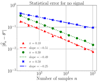
We summarize a few common aspects of the numerical experiments presented in the paper. Population-level computations were done using numerical integration on a sufficiently fine grid. With finite samples, the stopping criteria for the convergence of EM were: (1) the change in the iterates was small enough, or (2) the number of iterations was too large (greater than $100,000$). Experiments were averaged over several repetitions (ranging from $25$ to $400$). In majority of the runs, for each case, criteria (1) led to convergence. In our plots for sample EM, we report $\widehat{m}_{e}+2\widehat{s}_{e}$ on the y-axis, where $\widehat{m}_{e},\widehat{s}_{e}$ respectively denote the mean and standard deviation across the experiments for the metric under consideration, e.g., the parameter estimation error. Furthermore, whenever a slope is provided, it is the slope for the least-squares fit on the log-log scale for the quantity on $y$-axis when fitted with the quantity reported on the $x$-axis. For instance, in Figure 1(b), we plot $|\widehat{\theta}_{n}-\theta^{*}|$ on the $y$-axis value versus the sample size $n$ on the $x$-axis, averaged over $400$ experiments, accounting for the deviation across these experiments. Furthermore, the green dotted line with legend $\uppi=0.3$ and the corresponding slope $-0.48$ denote the least-squares fit and the respective slope for $\log|\widehat{\theta}_{n}-\theta^{*}|$ (green solid dots) with $\log n$ for the experiments corresponding to the setting $\uppi=0.3$.

2 Motivating simulations and problem set-up

In this section, we explore a wide range of behavior demonstrated by EM for certain settings of over-specified location Gaussian mixtures. We begin with several simulations that illustrate fast and slow convergence of EM for various settings, and serve as a motivation for the theoretical results derived later in the paper. We provide basic background on EM in Section 2.3, and describe the problems to be tackled.

2.1 Problem set-up

Let $\phi(\cdot\>;\mu,\Sigma)$ denote the density of a Gaussian random vector with mean $\mu$ and covariance $\Sigma$. Consider the two component Gaussian mixture model with density

$$f(x;\theta^{*},\sigma,\uppi) :=\uppi\phi(x;\theta^{*},\sigma^{2}I_{d})+(1-\uppi)\phi(x;-\theta^{*},\sigma^{2}I_{d}).$$ (1)

Given $n$ samples from the distribution (1), suppose that we use the EM algorithm to fit a two-component location Gaussian mixture with fixed weights and variance and special structure on the location parameters—more precisely, we fit the model with density

$$f(x;\theta,\sigma,\uppi) :=\uppi\phi(x;\theta,\sigma^{2}I_{d})+(1-\uppi)\phi(x;-\theta,\sigma^{2}I_{d})$$ (2)

using the EM algorithm, and take the solution as an estimate of $\theta^{*}$. An important aspect of the problem at hand is the signal strength, which is measured as the separation between the means of mixture components relative to the spread in the components. For the model (1), the signal strength is given by the ratio $\left\|\theta^{*}\right\|_{2}/\sigma$. When this ratio is large, we refer to it as the strong signal case; otherwise, it corresponds to the weak signal case. Of particular interest to us is the behavior of EM in the limit of weak signal when there is no separation; i.e., $\left\|\theta^{*}\right\|_{2}=0$. For such cases, we call the fit (2) an unbalanced fit when $\uppi\neq\frac{1}{2}$ and a balanced fit when $\uppi=\frac{1}{2}$. Note that the setting of $\theta^{*}=0$ corresponds to the simplest case of over-specified fit, since the true model has just one component (standard normal distribution irrespective of the parameter $\uppi$) but the fitted model has two (one extra) component (unless the EM estimate is also $0$). We now present the empirical behavior of EM for these models and defer the derivation of EM updates to Section 2.3.

2.2 Numerical Experiments: Fast to slow convergence of EM

We begin with a numerical study of the effect of separation among the mixtures on the statistical behavior of the estimates returned by EM. Our main observation is that weak or no separation leads to relatively low accuracy estimates. Additional simulations for more general mixtures, including more than two components, are provided in Section 5.3. Next, via numerical integration on a grid with sufficiently small discretization width, we simulate the behavior of the population EM algorithm width—an idealized version of EM in the limit of infinite samples—in order to understand the effect of signal strength on EM’s algorithmic rate of convergence, i.e., the number of steps needed for population EM to converge to a desired accuracy. We observe a slow down of EM on the algorithmic front when the signal strength approaches zero.

2.2.1 Effect of signal strength on sample EM

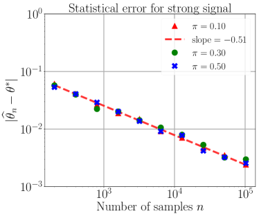
In Figure 1, we show simulation results for data generated from the model (1) in dimension $d=1$ and noise variance $\sigma^{2}=1$, and for three different values of the weight $\uppi\in\left\{0.1,0.3,0.5\right\}$. In all cases, we fit a two-location Gaussian mixture with fixed weights and variance as specified by equation (2). The two panels show the estimation error of the EM solution as a function of $n$ for two distinct cases of the data-generating mechanism: (a) in the strong signal case, we set $\theta^{*}=5$ so that the data has two well-separated mixture components, and (b) to obtain the limiting case of no signal, we set $\theta^{*}=0$, so that the two mixture components in the data-generating distribution collapse to one, and we are simply fitting the data from a standard normal distribution.

In the strong signal case, it is well known [1, 7] that EM solutions have an estimation error (measured by the Euclidean distance between the EM estimate and the true parameter $\theta^{*}$) that achieves the classical (parametric) rate $n^{-\frac{1}{2}}$; the empirical results in Figure 1(a) are simply a confirmation of these theoretical predictions. More interesting is the case of no signal (which is the limiting case with weak signal), where the simulation results shown in panel (b) of Figure 1 reveal a different story. In this case, whereas the EM solution (with random standard normal initialization) has an error that decays as $n^{-\frac{1}{2}}$ when $\uppi\neq 1/2$, its error decays at the considerably slower rate $n^{-\frac{1}{4}}$ when $\uppi=1/2$. We return to these cases in further detail in Section 3.

(a) $\theta^{*}=5$	(b) $\theta^{*}=0$

Figure 1: Plots of the error $|\widehat{\theta}_{n}-\theta^{*}|$ in the EM solution versus the sample size $n$, focusing on the effect of signal strength on EM solution accuracy. The true data distribution is given by $\uppi\mathcal{N}(\theta^{*},1)+(1-\uppi)\mathcal{N}(-\theta^{*},1)$ and we use EM to fit the model $\uppi\mathcal{N}(\theta,1)+(1-\uppi)\mathcal{N}(-\theta,1)$, generating the EM estimate $\widehat{\theta}_{n}$ based on $n$ samples. (a) When the signal is strong, the estimation rate decays at the parametric rate $n^{-\frac{1}{2}}$, as revealed by the $-1/2$ slope in a least-square fit of the log error based on the log sample size $\log n$. (b) When there is no signal ($\theta^{*}=0$), then depending on the choice of weight $\uppi$ in the fitted model, we observe two distinct scalings for the error: $n^{-\frac{1}{2}}$ when $\uppi\neq 0.5$, and, $n^{-\frac{1}{4}}$ when $\uppi=0.5$, again as revealed by least-squares fits of the log error using the log sample size $\log n$.

2.2.2 Interesting behavior of population EM

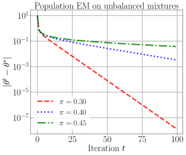
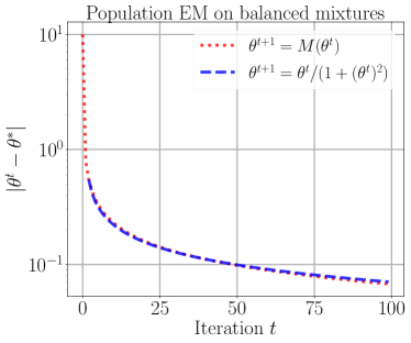
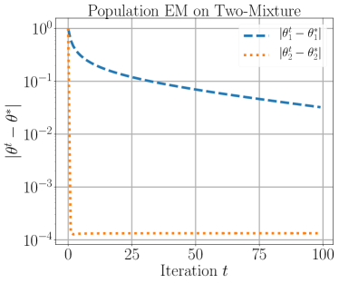
The intriguing behavior of the sample EM algorithm in the “no signal” case motivated us to examine the behavior of population EM for this case. To be clear, while sample EM is the practical algorithm that can actually be applied, it can be insightful for theoretical purposes to first analyze the convergence of the population EM updates, and then leverage these findings to understand the behavior of sample EM [1]. Our analysis follows a similar road-map. Interestingly, for the case with $\theta^{*}=0$, the population EM algorithm behaves significantly differently for the unbalanced fit ($\uppi\neq\frac{1}{2}$) as compared to the balanced fit ($\uppi=\frac{1}{2}$) (equation (2)). In Figure 2, we plot the distance of the population EM iterate $\theta^{t}$ to the true parameter value, $\theta^{*}=0$, on the vertical axis, versus the iteration number $t$ on the horizontal axis. With the vertical axis on a log scale, a geometric convergence rate of the algorithm shows up as a negatively sloped line (disregarding transient effects in the first few iterations).

(a)	(b)

Figure 2: Behavior of the (numerically computed) population EM updates (8) when the underlying data distribution is $\mathcal{N}(0,1)$. (a) Unbalanced mixture fits (2) with weights $(\uppi,1-\uppi)$: We observe geometric convergence towards $\theta^{*}=0$ for all $\uppi\neq 0.5$ although the rate of convergence gets slower as $\uppi\to 0.5$. (b) Balanced mixture fits (2) with weights $(0.5,0.5)$: We observe two phases of convergence. First, EM quickly converges to ball of constant radius and then it exhibits slow convergence towards $\theta^{*}=0$. Indeed, we see that during the slow convergence, the population EM updates track the curve given by $\theta^{t+1}=\theta^{t}/(1+(\theta^{t})^{2})$ very closely, as predicted by our theory.

For the unbalanced mixtures in panel (a), we see that EM converges geometrically quickly, although the rate of convergence (corresponding to the slope of the line) tends towards zero as the mixture weight $\uppi$ tends towards $1/2$ from below. For $\uppi=1/2$, we obtain a balanced mixture, and, as shown in the plot in panel (b), the convergence rate is now sub-geometric. In fact, the behavior of the iterates is extremely well characterized by the recursion $\theta\mapsto\frac{\theta}{1+\theta^{2}}$.

The theory to follow provides a precise characterization of the behavior seen in Figures 1(b) and 2. Furthermore, in Section 5, we provide further support for relevannce of our theoretical results in explaining the behavior of EM for other classes of over-specified models, including Gaussian mixture models with unknown weights as well as mixtures of linear regressions.

2.3 EM updates for the model fit (2)

In this section, we provide a quick introduction to the EM updates. Readers familiar with the literature can skip directly to the main results in Section 3. Recall that the two-component model fit is based on the density

$$\uppi\phi(x;\theta,\sigma^{2}I_{d})+(1-\uppi)\phi(x;-\theta,\sigma^{2}I_{d}).$$ (3)

From now on we assume that the data is drawn from the zero-mean Gaussian distribution $\mathcal{N}(0,\sigma^{2}I_{d})$. Note that the model fit described above contains the true model with $\theta^{*}=0$ and it is referred to as an over-specified fit since for any non-zero $\theta$, the fitted model has two components.

The maximum likelihood estimate is obtained by solving the following optimization problem

$$\widehat{\theta}_{n}^{\text{MLE}}\in\arg\max_{\theta\in\Theta}\frac{1}{n}\sum_{i=1}^{n}\left\{\log(\uppi\phi(x_{i};\theta,\sigma^{2}I_{d})+(1-\uppi)\phi(x_{i};-\theta,\sigma^{2}I_{d}))\right\}.$$ (4)

In general, there is no closed-form expression for $\widehat{\theta}_{n}^{\text{MLE}}$. The EM algorithm circumvents this problem via a minorization-maximization scheme. Indeed, population EM is a surrogate method to compute the maximizer of the population log-likelihood

$$\mathcal{L}(\theta):={\mathbb{E}}_{X}\left[\log(\uppi\phi(X;\theta,\sigma^{2}I_{d})+(1-\uppi)\phi(X;-\theta,\sigma^{2}I_{d})\right],$$ (5)

where the expectation is taken over the true distribution. On the other hand, sample EM attempts to estimate $\widehat{\theta}_{n}^{\text{MLE}}$. We now describe the expressions for both the sample and population EM updates for the model-fit (3).

Given any point $\theta$, the EM algorithm proceeds in two steps: (1) compute a surrogate function $Q(\cdot;\theta)$ such that $Q(\theta^{\prime};\theta)\leq\mathcal{L}(\theta^{\prime})$ and $Q(\theta;\theta)=\mathcal{L}(\theta)$; and (2) compute the maximizer of $Q(\theta^{\prime};\theta)$ with respect to $\theta^{\prime}$. These steps are referred to as the E-step and the M-step, respectively. In the case of two-component location Gaussian mixtures, it is useful to describe a hidden variable representation of the mixture model. Consider a binary indicator variable $Z\in\left\{0,1\right\}$ with the marginal distribution ${\mathbb{P}}(Z=1)=\uppi$ and ${\mathbb{P}}(Z=0)=1-\uppi$, and define the conditional distributions

$$\left(X\mid Z=0\right)\sim\mathcal{N}(-\theta,\sigma^{2}I_{d}),\quad\text{and}\quad\left(X\mid Z=1\right)\sim\mathcal{N}(\theta,\sigma^{2}I_{d}).$$

These marginal and conditional distributions define a joint distribution over the pair $(X,Z)$, and by construction, the induced marginal distribution over $X$ is a Gaussian mixture of the form (3). For EM, we first compute the conditional probability of $Z=1$ given $X=x$:

$$w_{\theta}(x)=w^{\uppi}_{\theta}(x):=\frac{\uppi\exp\left(-\frac{\left\|\theta-x\right\|_{2}^{2}}{2\sigma^{2}}\right)}{\uppi\exp\left(-\frac{\left\|\theta-x\right\|_{2}^{2}}{2\sigma^{2}}\right)+(1-\uppi)\exp\left(-\frac{\left\|\theta+x\right\|_{2}^{2}}{2\sigma^{2}}\right)}.$$ (6)

Then, given a vector $\theta$, the E-step in the population EM algorithm involves computing the minorization function $\theta^{\prime}\mapsto Q(\theta^{\prime},\theta)$. Doing so is equivalent to computing the expectation

$$Q(\theta^{\prime};\theta) =-\frac{1}{2}{\mathbb{E}}\left[w_{\theta}(X)\left\|X-\theta^{\prime}\right\|_{2}^{2}+(1-w_{\theta}(X))\left\|X+\theta^{\prime}\right\|_{2}^{2}\right],$$ (7)

where the expectation is taken over the true distribution (here $\mathcal{N}(0,\sigma^{2}I_{d})$. In the M-step, we maximize the function $\theta^{\prime}\mapsto Q(\theta^{\prime};\theta)$. Doing so defines a mapping $M:\mathbb{R}^{d}\to\mathbb{R}^{d}$, known as the population EM operator, given by

$$M(\theta) =\arg\max_{\theta^{\prime}\in\mathbb{R}^{d}}Q(\theta^{\prime},\theta)={\mathbb{E}}\Big{[}(2w_{\theta}(X)-1)X\Big{]}.$$ (8)

In this definition, the second equality follows by computing the gradient $\nabla_{\theta^{\prime}}Q$, and setting it to zero. In summary, for the two-component location mixtures considered in this paper, the population EM algorithm is defined by the sequence $\theta^{t+1}=M(\theta^{t})$, where the operator $M$ is defined in equation (8).

We obtain the sample EM update by simply replacing the expectation ${\mathbb{E}}$ in equations (7) and (8) by the empirical average based on an observed set of samples. In particular, given a set of i.i.d. samples $\left\{X_{i}\right\}_{i=1}^{n}$, the sample EM operator $M_{n}:{}^{d}\mapsto{}^{d}$ takes the form

$$M_{n}(\theta) :=\frac{1}{n}\sum_{i=1}^{n}(2w_{\theta}(X_{i})-1)X_{i}.$$ (9)

Overall, the sample EM algorithm generates the sequence of iterates given by $\theta^{t+1}=M_{n}(\theta^{t})$.

In the sequel, we study the convergence of EM both for the population EM algorithm in which the updates are given by $\theta^{t+1}=M(\theta^{t})$, and the sample-based EM sequence given by $\theta^{t+1}=M_{n}(\theta^{t})$. With this notation in place, we now turn to the main results of this paper.

3 Main results

In this section, we state our main results for the convergence rates of the EM updates under the unbalanced and balanced mixture fit. We start with the easier case of unbalanced mixture fit in Section 3.1 followed by the more delicate (and interesting) case of the balanced fit in Section 3.2.

3.1 Behavior of EM for unbalanced mixtures

We begin with a characterization of both the population and sample-based EM updates in the setting of unbalanced mixtures. In particular, we assume that the fitted two-components mixture model (3) has known weights $\uppi$ and $1-\uppi$, where $\uppi\in(0,1/2)$. The following result characterizes the behavior of the EM updates for this set-up.

Theorem 1.

Suppose that we fit an unbalanced instance (i.e., $\uppi\neq\frac{1}{2}$) of the mixture model (3) to $\mathcal{N}(0,\sigma^{2}I_{d})$ data. Then:

1. The population EM operator (8) is globally strictly contractive, meaning that

   $$\left\|M(\theta)\right\|_{2} \leq\left(1-\rho^{2}/2\right)\left\|\theta\right\|_{2}\qquad\mbox{for all $\theta\in{}^{d}$,}$$ (10a)

   where $$\rho:=|1-2\uppi|\in(0,1)$$.

2. There are universal constants $c,c^{\prime}$ such that given any $\delta\in(0,1)$ and a sample size $n\geq c\frac{\sigma^{2}}{\rho^{4}}\,(d+\log(1/\delta))$, the sample EM sequence $\theta^{t+1}=M_{n}(\theta^{t})$ generated by the update (9) satisfies the upper bound

   $$\left\|\theta^{t}\right\|_{2}\leq\left\|\theta^{0}\right\|_{2}\left(1-\frac{\rho^{2}}{2}\right)^{t}+\frac{c^{\prime}(\left\|\theta^{0}\right\|_{2}\sigma^{2}+\rho\sigma)}{\rho^{2}}\sqrt{\frac{d+\log(1/\delta)}{n}}\;,$$ (10b)

   with probability at least $1-\delta$.

See Appendix A.1 for the proof of this theorem.

Fast convergence of population EM

The bulk of the effort in proving Theorem 1 lies in establishing the guarantee (10a) for the population EM iterates. Such a contraction bound immediately yields the exponential fast convergence of the population EM updates $\theta^{t+1}=M(\theta^{t})$ to $\theta^{*}=0$:

$$\left\|\theta^{T}\right\|_{2}\leq\epsilon\quad\text{for }\quad T\geq\frac{1}{\log\frac{1}{(1-\rho^{2}/2)}}\cdot{\log\left(\frac{\left\|\theta^{0}\right\|_{2}}{\epsilon}\right)}.$$ (11)

Since the mixture weights $(\uppi,1-\uppi)$ are bounded away from $1/2$, we have that $\rho=|1-2\uppi|$ is bounded away from zero, and thus population EM iterates converge in $\mathcal{O}\left(\log(1/\epsilon)\right)$ steps to an $\epsilon$-ball around $\theta^{*}=0$. This result is equivalent to showing that in the unbalanced instance $(\uppi\neq 1/2)$, the log-likelihood is strongly concave around the true parameter.

Statistical rate of sample EM

Once the bounds (10a) and (11)) have been established, the proof of the statistical rate (10b) for sample EM utilizes the scheme laid out by Balakrishnan et al. [1]. In particular, we prove a non-asymptotic uniform law of large numbers (Lemma 1 stated in Section 4.1) that allows for the translation from population to sample EM iterates. Roughly speaking, Lemma 1 guarantees that for any radius $r>0$, tolerance $\delta\in(0,1)$, and sufficiently large $n$, we have

$${\mathbb{P}}\left[\sup\limits_{\|\theta\|_{2}\leq r}\left\|M_{n}(\theta)-M(\theta)\right\|_{2}\leq c_{2}\sigma(\sigma r+\rho)\sqrt{\frac{d+\log(1/\delta)}{n}}\;\right]\geq 1-\delta.$$ (12)

This bound, when combined with the contractive behavior (10a) or equivalently the exponentially fast convergence (11) of the population EM iterates allows us to establish the stated bound (10b). (See, e.g., Theorem 2 in the paper [1].)

Putting the pieces together, we conclude that the sample EM updates converge to an estimate of $\theta^{*}$—that has Euclidean error of the order $(d/n)^{\frac{1}{2}}$—after a relatively small number of steps that are of the order $\log(n/d)$. Note that this theoretical prediction is verified by the simulation study in Figure 1(b) for the univariate setting ($d=1$) of the unbalanced mixture-fit. In Figure 3, we present the scaling of the radius of the final EM iterate with respect to the sample size $n$ and the dimension $d$, averaged over $400$ runs of sample EM for various settings of $(n,d)$. Linear fits on the log-log scale in these simulations suggest a rate close to $(d/n)^{\frac{1}{2}}$ as claimed in Theorem 1.

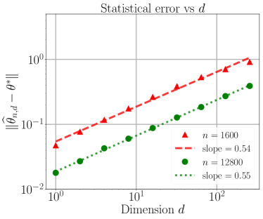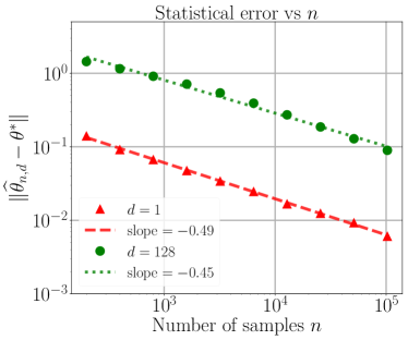(a)	(b)

Figure 3: Scaling of the Euclidean error $\|\widehat{\theta}_{n,d}-\theta^{*}\|_{2}$ for EM estimates $\widehat{\theta}_{n,d}$ computed using the unbalanced ($\uppi\neq\frac{1}{2}$) mixture-fit (3). Here the true data distribution is $\mathcal{N}(0,I_{d})$, i.e., $\theta^{*}=0$, and $\widehat{\theta}_{n,d}$ denotes the EM iterate upon convergence when we fit a two-mixture model with mixture weights $(0.3,0.7)$ using $n$ samples in $d$ dimensions. (a) Scaling with respect to $d$ for $n\in\left\{1600,12800\right\}$. (b) Scaling with respect to $n$ for $d\in\left\{1,128\right\}$. We ran experiments for several other pairs of $(n,d)$ and the conclusions were the same. The empirical results here show that that our theoretical upper bound of the order $(d/n)^{\tfrac{1}{2}}$ on the EM solution is sharp in terms of $n$ and $d$.

Remark

We make two comments in passing. First, the value of $\left\|\theta^{0}\right\|_{2}$ in the convergence rate of sample EM updates in Theorem 1 can be assumed to be of constant order; this assumption stems from the fact the population EM operator maps any $\theta^{0}$ to a vector with norm smaller than $\sqrt{2/\pi}$ (cf. Lemma 5 in Appendix C.1). Second, when the weight parameter $\uppi$ is assumed to be unknown in the model fit (3), the EM algorithm exhibits fast convergence when $\uppi$ is initialized sufficiently away from $\frac{1}{2}$; see Section 5.1 for more details.

From unbalanced to balanced fit

The bound (11) shows that the extent of unbalancedness in the mixture weights plays a crucial role in the geometric rate of convergence for the population EM. When the mixtures become more balanced, that is, weight $\uppi$ approaches $1/2$ or equivalently $\rho$ approaches zero, the number of steps $T$ required to achieve $\epsilon$-accuracy scales as $\mathcal{O}\left({\log(\left\|\theta^{0}\right\|_{2}/\epsilon)}/{\rho^{2}}\right)$ and in the limit $\rho\rightarrow 0$, this bound degenerates to $\infty$ for any finite $\epsilon$. Indeed, the bound (10a) from Theorem 1 simply states that the population EM operator is non-expansive for balanced mixtures ($\rho=0$), and does not provide any particular rate of convergence for this case. It turns out that the EM algorithm is worse in the balanced case, both in terms of the optimization speed and in terms of the statistical rate. This slower statistical rate is in accord with existing results for the MLE in over-specified mixture models [4]; the novel contribution here is the rigorous analysis of the analogous behavior for the EM algorithm.

3.2 Behavior of EM for balanced mixtures

In this section, we first provide a sharp characterization of the algorithmic rate of convergence of the population EM update for the balanced fit (see Section 3.2.1). We then provide sharp bound for the statistical rate for the sample EM updates (cf. Section 3.2.2).

3.2.1 Slow convergence of population EM

We now analyze the behavior of the population EM operator for the balanced fit. We show that it is globally convergent, albeit with a contraction parameter that depends on $\theta$, and degrades towards $1$ as $\|\theta\|_{2}\rightarrow 0$. Our statement involves the constant $p:={\mathbb{P}}(\left|X\right|\leq 1)+\frac{1}{2}{\mathbb{P}}(\left|X\right|>1)$, where $X\sim\mathcal{N}(0,1)$ denotes a standard normal variate. (Note that $p<1$.)

Theorem 2.

Suppose that we fit a balanced instance ($\uppi=\frac{1}{2}$) of the mixture model (3) to $\mathcal{N}(0,\sigma^{2}I_{d})$ data. Then the population EM operator (8) ${\theta\mapsto M(\theta)}$ has the following properties:

1. For all non-zero $\theta$, we have

   $$\frac{\left\|M(\theta)\right\|_{2}}{\left\|\theta\right\|_{2}} \leq\gamma_{\textrm{up}}(\theta)\;:=1-p+\frac{p}{1+\frac{\left\|\theta\right\|_{2}^{2}}{2\sigma^{2}}}\;<\;1.$$ (13a)

2. For all non-zero $\theta$ such that $\left\|\theta\right\|_{2}^{2}\leq\frac{5\sigma^{2}}{8}$, we have

   $$\frac{\left\|M(\theta)\right\|_{2}}{\left\|\theta\right\|_{2}} \geq\gamma_{\textrm{low}}(\theta)\;:=\;\frac{1}{1+\frac{2\left\|\theta\right\|_{2}^{2}}{\sigma^{2}}}.$$ (13b)

See Appendix A.2 for the proof of Theorem 2.

The salient feature of Theorem 2 is that the contraction coefficient $\gamma_{\textrm{up}}(\theta)$ is not globally bounded away from $1$ and in fact satisfies $\lim_{\theta\rightarrow 0}\gamma_{\textrm{up}}(\theta)=1$. In conjunction with the lower bound (13b), we see that

$$\frac{\left\|M(\theta)\right\|_{2}}{\left\|\theta\right\|_{2}} \asymp\left(1-\frac{\left\|\theta\right\|_{2}^{2}}{\sigma^{2}}\right)\qquad\mbox{for small $\left\|\theta\right\|_{2}$.}$$ (14)

This precise contraction behavior of the population EM operator is in accord with that of the simulation study in Figure 2(b).

The preceding results show that the population EM updates should exhibit two phases of behavior. In the first phase, up to a relatively coarse accuracy of the order $\sigma$, the iterates exhibit geometric convergence. Concretely, we are guaranteed to have $\left\|\theta^{T_{0}}\right\|_{2}\leq\sqrt{2}\sigma$ after running the algorithm for $T_{0}:=\frac{\log(\left\|\theta^{0}\right\|_{2}^{2}/(2\sigma^{2}))}{\log(2/(2-p))}$ steps. In the second phase, as the error decreases from $\sqrt{2}\sigma$ to a given $\epsilon\in\big{(}0,\sqrt{2}\sigma\big{)}$, the convergence rate becomes sub-geometric; concretely, we have

$$\left\|\theta^{T_{0}+t}\right\|_{2} \leq\,\epsilon\quad\text{for}\quad t\geq\frac{c\sigma^{2}}{\epsilon^{2}}\log(\sigma/\epsilon).$$ (15)

Note that the conclusion (15) shows that for small enough $\epsilon$, the population EM takes $\Theta(\log(1/\epsilon)/\epsilon^{2})$ steps to find $\epsilon$-accurate estimate of $\theta^{*}=0$. This rate is extremely slow compared to the geometric rate $\mathcal{O}(\log(1/\epsilon))$ derived for the unbalanced mixtures in Theorem 1. Hence, the slow rate establishes a qualitative difference in the behavior of the EM algorithm between the balanced and unbalanced setting.

Moreover, the sub-geometric rate of EM in the balanced case is also in stark contrast with the favorable behavior of EM for the exact-fitted settings analyzed in past work. Balakrishnan et al. [1] showed that when the EM algorithm is used to fit a two-component Gaussian mixture with sufficiently large value of $\frac{\left\|\theta^{\star}\right\|_{2}}{\sigma}$ (known as the high signal-to-noise ratio, or high SNR for short), the population EM operator is contractive, and hence geometrically convergent, within a neighborhood of the true parameter $\theta^{*}$. In a later work on the two-component balanced mixture fit model, Daskalakis et al. [7] showed that the convergence is in fact geometric for any non-zero value of the SNR. The model considered in Theorem 2 can be seen as the limiting case of weak signal for a two mixture model—which degenerates to the Gaussian distribution when the SNR becomes exactly zero. For such a limit, we observe that the fast convergence of population EM sequence no longer holds.

3.2.2 Upper and lower bounds on sample EM

We now turn to the statements of upper and lower bounds on the rate of the sample EM iterates for the balanced fit on Gaussian data. We begin with an upper bound, which involves the previously defined function $\gamma_{\textrm{up}}(\theta)\;:=1-p+p/\big{(}{1+\frac{\left\|\theta\right\|_{2}^{2}}{2\sigma^{2}}}\big{)}$.

Theorem 3.

Consider the sample EM updates $\theta^{t}=M_{n}(\theta^{t-1})$ for the balanced instance ($\uppi=\frac{1}{2}$) of the mixture model (3) based on $n$ i.i.d. $\mathcal{N}(0,\sigma^{2}I_{d})$ samples. Then, there exist universal constants $\left\{c^{\prime}_{k}\right\}_{k=1}^{4}$ such that for any scalars $\alpha\in(0,\frac{1}{4})$ and $\delta\in(0,1)$, any sample size $n\geq c^{\prime}_{1}(d+\log(\log(1/\alpha)/\delta))\;$ and any iterate number $t\geq c^{\prime}_{2}\log\frac{\|{\theta^{0}}\|^{2}n}{\sigma^{2}d}+c^{\prime}_{3}\left(\frac{n}{d}\right)^{\frac{1}{2}-2\alpha}\log(\frac{n}{d})\log(\frac{1}{\alpha})$, we have

$$\|\theta^{t}\|_{2}\leq\left[\left\|\theta^{0}\right\|_{2}\cdot\prod_{j=0}^{t-1}\gamma_{\textrm{up}}(\theta^{j})\right]+c^{\prime}_{4}\sigma\left(\frac{\sigma^{2}(d+\log\frac{\log(4/\epsilon)}{\delta})}{n}\right)^{\frac{1}{4}-\alpha},$$ (16)

with probability at least $1-\delta$.

See Section 4 for a discussion of the techniques employed to prove this theorem. The detailed proof is provided in Appendix A.3, where we also provide some more details on the definitions of these constants.

As we show in our proofs, once the iteration number $t$ satisfies the lower bound stated in the theorem, the second term on the right-hand side of the bound (16) dominates the first term; therefore, from this point onwards, the the sample EM iterates have Euclidean norm of the order $(d/n)^{\frac{1}{4}-\alpha}$. Note that $\alpha\in(0,\frac{1}{4})$ can be chosen arbitrarily close to zero, so at the expense of increasing the lower bound on the number of iterations $t$ by a logarithmic factor $\log(1/\alpha)$, we can obtain rates arbitrarily close to $(d/n)^{\frac{1}{4}}$.

We note that earlier studies of parameter estimation for over-specified mixtures, in both the frequentist [4] and Bayesian settings [15, 23], have derived a rate of $n^{-\frac{1}{4}}$ for the global maximum of the log likelihood. To the best of our knowledge, Theorem 3 is the first non-asymptotic algorithmic result that shows that such rates apply to the fixed points and dynamics of the EM algorithm, which need not converge to the global optima.

The preceding discussion was devoted to an upper bound on sample EM for the balanced fit. Let us now match this upper bound, at least in the univariate case $d=1$, by showing that any non-zero fixed point of the sample EM updates has Euclidean norm of the order $n^{-\frac{1}{4}}$. In particular, we prove the following lower bound.

Theorem 4.

There are universal positive constants $c,c^{\prime}$ such that for any non-zero solution $\widehat{\theta}_{n}$ to the sample EM fixed-point equation $\theta=M_{n}(\theta)$ for the balanced mixture fit, we have

$${\mathbb{P}}\left[|{\widehat{\theta}_{n}}|\geq c\,n^{-\frac{1}{4}}\right]\geq c^{\prime}.$$ (17)

See Appendix A.4 for the proof of this theorem.

Since the iterative EM scheme converges only to one of its fixed points, the theorem shows that one cannot obtain a high-probability bound for any radius smaller than $n^{-\frac{1}{4}}$. As a consequence, with constant probability, the radius of convergence $n^{-\frac{1}{4}}$ for sample EM convergence in Theorem 3 for the univariate setting is tight.

4 New techniques for sharp analysis of sample EM

In this section, we highlight the new proof techniques introduced in this work that are required to obtain the sharp characterization of the sample EM updates in the balanced case (Theorem 3). We begin in Section 4.1 by elaborating that a direct application of the previous frameworks leads to sub-optimal statistical rates for sample EM in the balanced fit. This sub-optimality motivates the development of new methods for analyzing the behavior of the sample EM iterates, based on an annulus-based localization argument over a sequence of epochs, which we sketch out in Sections 4.2 and 4.3. We remark that our novel techniques, introduced here for analyzing EM with the balanced fit, are likely to be of independent interest. We believe that they can potentially be extended to derive sharp statistical rates in other settings when the algorithm under consideration does not exhibit an geometrically fast convergence.

4.1 A sub-optimal guarantee

Let us recall the set-up for the procedure suggested by Balakrishnan et al. [1], specializing to the case where the true parameter $\theta^{*}=0$, as in our specific set-up. Using the triangle inequality, the norm of the sample EM iterates $\theta^{t+1}=M_{n}(\theta^{t})$ can be upper bounded by a sum of two terms as follows:

$$\left\|\theta^{t+1}\right\|_{2}=\left\|M_{n}(\theta^{t})\right\|_{2}\leq\left\|M_{n}(\theta^{t})-M(\theta^{t})\right\|_{2}+\left\|M(\theta^{t})\right\|_{2}$$ (18)

for all $t\geq 0$. The first term on the right-hand side corresponds to the deviations between the sample and population EM operators, and can be controlled via empirical process theory. The second term corresponds to the behavior of the (deterministic) population EM operator, as applied to the sample EM iterate $\theta^{t}$, and needs to be controlled via a result on population EM.

Theorem 2 from Balakrishnan et al. [1] is based on imposing generic conditions on each of these two terms, and then using them to derive a generic bound on the sample EM iterates. In the current context, their theorem can be summarized as follows. For given tolerances $\delta\in(0,1)$, $\epsilon>0$ and starting radius $r>0$, suppose that there exists a function $\varepsilon(n,\delta)>0$, decreasing in terms of the sample size $n$, and a contraction coefficient $\kappa\in(0,1)$ such that

$$\sup_{\left\|\theta\right\|_{2}\geq\epsilon}\frac{\left\|M(\theta)\right\|_{2}}{\left\|\theta\right\|_{2}}\!\leq\!\kappa\text{ and }{\mathbb{P}}\left[\sup_{\left\|\theta\right\|_{2}\leq r}\left\|M_{n}(\theta)\!-\!M(\theta)\right\|_{2}\!\leq\!\varepsilon(n,\delta)\right]\!\geq\!1\!-\!\delta.$$ (19a)

Then for a sample size $$n \epsilon$$ sufficiently large and sufficiently small to ensure that

$$\epsilon\;\stackrel{{\scriptstyle(i)}}{{\leq}}\;\frac{\varepsilon(n,\delta)}{1-\kappa}\;\stackrel{{\scriptstyle(ii)}}{{\leq}}\;r,$$ (19b)

the sample EM iterates are guaranteed to converge to a ball of radius ${\varepsilon(n,\delta)}/({1-\kappa})$ around the true parameter $\theta^{*}=0$.

In order to apply this theorem to the current setting, we need to specify a choice of $\varepsilon(n,\delta)$ for which the bound on the empirical process holds. The following auxiliary result provides such control for us:

Lemma 1.

There exists universal positive constants $c_{1}$ and $c_{2}$ such that for any positive radius $r$, any threshold $\delta\in(0,1)$, and any sample size $n\geq c_{2}d\log(1/\delta)$, we have

$${\mathbb{P}}\left[\sup\limits_{\|\theta\|_{2}\leq r}\left\|M_{n}(\theta)-M(\theta)\right\|_{2}\leq c_{1}\sigma(\sigma r+\rho)\sqrt{\frac{d+\log(1/\delta)}{n}}\right]\geq 1-\delta,$$ (20)

where $\rho=\left|1-2\uppi\right|$ denotes the imbalance in the mixture fit (3).

The proof of this lemma is based on Rademacher complexity arguments; see Appendix B.1 for the details.

With the choice $r=\left\|\theta^{0}\right\|_{2}$, Lemma 1 guarantees that the second inequality in line (19a) holds with $\varepsilon(n,\delta)\lesssim\sigma^{2}\left\|\theta^{0}\right\|_{2}\sqrt{d/n}$. On the other hand, Theorem 2 implies that for any $\theta$ such that $\left\|\theta\right\|_{2}\geq\epsilon$, we have that population EM is contractive with parameter bounded above by $\kappa(\epsilon)\asymp 1-\epsilon^{2}$. In order to satisfy inequality (i) in equation (19b), we solve the equation ${\varepsilon(n,\delta)}/({1-\kappa(\epsilon)})=\epsilon$. Tracking only the dependency on $d$ and $n$, we obtain

$$\frac{\sqrt{d/n}}{\epsilon^{2}}=\epsilon\quad\Longrightarrow\quad\epsilon=\mathcal{O}\left((d/n)^{\frac{1}{6}}\right),$$ (21)

which shows that the Euclidean norm of the sample EM iterate is bounded by a term of order $(d/n)^{\frac{1}{6}}$.

While this rate is much slower than the classical $(d/n)^{\frac{1}{2}}$ rate that we established in the unbalanced case, it does not coincide with the $n^{-\frac{1}{4}}$ rate that we obtained in Figure 1(b) for balanced setting with $d=1$. Thus, the proof technique based on the framework of Balakrishnan et al. [1] appears to be non-optimal. The sub-optimality of this approach necessitates the development of a more refined technique. Before sketching this technique, we now quantify empirically the convergence rate of sample EM in terms of both dimension $d$ and sample size $n$ for the balanced mixture fit. In Figure 4, we summarize the results of these experiments. The two panels in the figure exhibit that the error in the sample EM estimate scales as $(d/n)^{\frac{1}{4}}$, thereby providing further numerical evidence that the preceding approach indeed led to a sub-optimal result.

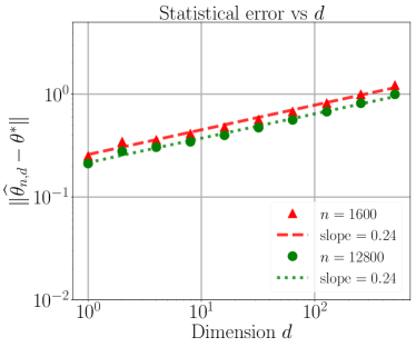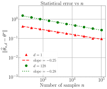(a)	(b)

Figure 4: Scaling of the Euclidean error $\|\widehat{\theta}_{n,d}-\theta^{*}\|_{2}$ for EM estimates $\widehat{\theta}_{n,d}$ computed using the balanced ($\uppi=\frac{1}{2}$) mixture-fit (2). Here the true data distribution is $\mathcal{N}(0,I_{d})$, i.e., $\theta^{*}=0$, and $\widehat{\theta}_{n,d}$ denotes the EM iterate upon convergence when we fit a balanced mixture with $n$ samples in $d$ dimensions. (a) Scaling with respect to $d$ for $n\in\left\{1600,12800\right\}$. (b) Scaling with respect to $n$ for $d\in\left\{1,128\right\}$. We ran experiments for several other pairs of $(n,d)$ and the conclusions were the same. Clearly, the empirical results suggest a scaling of order $(d/n)^{\frac{1}{4}}$ for the final iterate of sample-based EM.

(a)	(b)

Figure 5: Illustration of the annulus-based-localization argument part (I): Defining the epochs or equivalently the annuli. (a) Outer radius for the $\ell$-th epoch is given by $n^{-\alpha_{\ell}}$ (tracking dependency only on $n$). (b) For any given epoch $\ell$, we analyze the behavior of the EM sequence $\theta^{t+1}=M_{n}(\theta^{t})$, when $\theta^{t}$ lies in the annulus around $\theta^{*}$ with inner and outer radii given by $n^{-\alpha_{\ell+1}}$, and $n^{-\alpha_{\ell}}$, respectively. We prove that EM iterates move from one epoch to the next epoch (e.g. epoch $\ell$ to epoch $\ell+1$) after at most $\sqrt{n}$ iterations. Given the definition of $\alpha_{\ell}$, we see that the inner and outer radii of the aforementioned annulus converges linearly to $n^{-\frac{1}{4}}$. Consequently, after at most $\log(1/\alpha)$ epochs (or $\sqrt{n}\log(1/\alpha)$ iterations), the EM iterate lies in a ball of radius $n^{-{1}/{4}+\alpha}$ around $\theta^{*}$. We illustrate the one-step dynamics in any given annulus in Figure 6.

Figure 6: Illustration of the annulus-based-localization argument part (II): Dynamics of EM in the $\ell$-th epoch or equivalently the annulus $n^{-\alpha_{\ell+1}}\leq\|\theta^{t}-\theta^{*}\|_{2}\leq n^{-\alpha_{\ell}}.$ For a given epoch $\ell$, we analyze the behavior of the EM sequence $\theta^{t+1}=M_{n}(\theta^{t})$, when $\theta^{t}$ lies in the annulus with inner and outer radii given by $n^{-\alpha_{\ell+1}}$, and $n^{-\alpha_{\ell}}$, respectively. In this epoch, the population EM operator $M(\theta^{t})$ contracts with a contraction coefficient that depends on $n^{-\alpha_{\ell+1}}$, which is the inner radius of the disc, while the perturbation error ${\|M_{n}(\theta^{t})-M(\theta)\|_{2}}$ between the sample and population EM operators depends on $n^{-\alpha_{\ell}}$, which is the outer radius of the disc. Overall, we prove that $M_{n}$ is non-expansive and after at most $\sqrt{n}$ steps, the sample EM updates move from epoch $\ell$ to epoch $\ell+1$.

4.2 Annulus-based localization over epochs

Let us try to understand why the preceding argument led to a sub-optimal bound. In brief, its “one-shot” nature contains two major deficiencies. First, the tolerance parameter $\epsilon$ is used both (a) for measuring the contractivity of the updates, as in the first inequality in equation (19a), and (b) for determining the final accuracy that we achieve. At earlier phases of the iteration, the algorithm will converge more quickly than suggested by the worst-case analysis based on the final accuracy. A second deficiency is that the argument uses the radius $r$ only once, setting it to a constant to reflect the initialization $\theta^{0}$ at the start of the algorithm. This means that we failed to “localize” our bound on the empirical process in Lemma 1. At later iterations of the algorithm, the norm $\left\|\theta^{t}\right\|_{2}$ will be smaller, meaning that the empirical process can be more tightly controlled. We note that ideas of localizing the radius $r$ for an empirical process plays a crucial role in obtaining sharp bounds on the error of $M$-estimation procedures [28, 2, 18, 32].

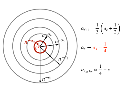
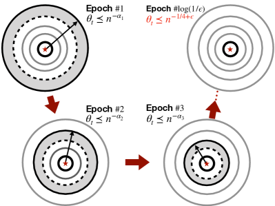
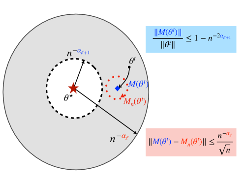
A novel aspect of the localization argument in our setting is the use of an annulus instead of a ball. In particular, we analyze the iterates from the EM algorithm assuming that they lie within a pre-specicied annulus, defined by an inner and an outer radius. On one hand, the outer radius of the annulus helps to provide a sharp control on the perturbation bounds between the population and sample operators. On the other hand, the inner radius of the annulus is used to tightly control the algorithmic rate of convergence.

We now summarize our key arguments. The entire sequence of sample EM iterations is broken up into a sequence of different epochs. During each epoch, we localize the EM iterates to an annulus. In more detail:

• We index epochs by the integer $\ell=0,1,2,\ldots$, and associate them with a sequence $\{\alpha_{\ell}\}_{\ell\geq 0}$ of scalars in the interval $[0,\frac{1}{4}]$. The input to epoch $\ell$ is the scalar $\alpha_{\ell}$, and the output from epoch $\ell$ is the scalar $\alpha_{\ell+1}$.

• The $\ell$-th epoch is defined to be the set of all iterations $t$ of the sample EM algorithm such that the sample EM iterate $\theta^{t}$ lies in the following annulus:

  $$\left(\frac{d}{n}\right)^{\alpha_{\ell+1}}\leq\|\theta^{t}-\theta^{*}\|_{2}\leq\left(\frac{d}{n}\right)^{\alpha_{\ell}}.$$ (22)

  We establish that the sample-EM operator is non-expansive so that each epoch is well-defined (and that subsequent iterations can only correspond to subsequent epochs).

• Upon completion of epoch $\ell$ at iteration $T_{\ell}$, the EM algorithm returns an estimate $\theta^{T_{\ell}}$ such that $\|\theta^{T_{\ell}}\|_{2}\precsim(d/n)^{\alpha_{\ell+1}}$, where

  $$\alpha_{\ell+1}=\frac{1}{3}\alpha_{\ell}+\frac{1}{6}.$$ (23)

  Note that the new scalar $\alpha_{\ell+1}$ serves as the input to epoch $\ell+1$.

The recursion (23) is crucial in our analysis: it tracks the evolution of the exponent acting upon the ratio $d/n$, and the rate $(d/n)^{\alpha_{\ell+1}}$ is the bound on the Euclidean norm of the sample EM iterates achieved at the end of epoch $\ell$.

A few properties of the recursion (23) are worth noting. First, given our initialization $\alpha_{0}=0$, we see that $\alpha_{1}=\frac{1}{6}$, which agrees with the outcome of our one-step analysis from above. Second, as the recursion is iterated, it converges from below to the fixed point $\alpha^{*}=\frac{1}{4}$. Thus, our argument will allow us to prove a bound arbitrarily close to $(d/n)^{\frac{1}{4}}$, as stated formally in Theorem 3 to follow. Refer to Figures 5 and 6 for an illustration of the definition of these annuli, epochs and the associated conclusions.

4.3 How does the key recursion (23) arise?

Let us now sketch out how the key recursion (23) arises. Consider epoch $\ell$ specified by input $\alpha_{\ell}<\frac{1}{4}$, and consider an iterate $\theta^{t}$ in the following annulus: $\left\|\theta^{t}\right\|_{2}\in[(d/n)^{\alpha_{\ell+1}},(d/n)^{\alpha_{\ell}}]$. We begin by proving that this initial condition ensures that $\left\|\theta^{t}\right\|_{2}$ is less than level $(d/n)^{\alpha_{\ell}}$ for all future iterations; for details, see Lemma 4 stated in the Appendix. Given this guarantee, our second step is to make use of the inner radius of the considered annulus to apply Theorem 2 for the population EM operator, for all iterations $t$ such that $\left\|\theta^{t}\right\|_{2}\geq(d/n)^{\alpha_{\ell+1}}$. Consequently, for these iterations, we have

$$\left\|M(\theta^{t})\right\|_{2} \leq\Big{(}1-p+\frac{p}{1+\frac{\left\|\theta\right\|_{2}^{2}}{2\sigma^{2}}}\Big{)}\left\|\theta^{t}\right\|_{2}$$

$$\precsim(1-(d/n)^{2\alpha_{\ell+1}})(d/n)^{\alpha_{\ell}}\leq\widetilde{\gamma}\;\left(\frac{d}{n}\right)^{\alpha_{\ell}},$$ (24a)

where $$\widetilde{\gamma}:=e^{-(d/n)^{2\alpha_{\ell+1}}}$$. On the other hand, using the outer radii of the annulus and applying Lemma 1 for this epoch, we obtain that

$$\left\|M_{n}(\theta^{t})-M(\theta^{t})\right\|_{2}\precsim\left(\frac{d}{n}\right)^{\alpha_{\ell}}\sqrt{\frac{d}{n}}=\left(\frac{d}{n}\right)^{\alpha_{\ell}+1/2},$$ (24b)

for all $t$ in the epoch. Unfolding the basic triangle inequality (18) for $T$ steps, we find that

$$\left\|\theta^{t+T}\right\|_{2} \leq\left\|M_{n}(\theta^{t})-M(\theta^{t})\right\|_{2}(1+\widetilde{\gamma}+\ldots+\widetilde{\gamma}^{T-1})+\widetilde{\gamma}^{T}\left\|\theta_{t}\right\|_{2}$$

$$\leq\frac{1}{1-\widetilde{\gamma}}\left\|M_{n}(\theta^{t})-M(\theta^{t})\right\|_{2}+e^{-T(d/n)^{2\alpha_{\ell+1}}}(d/n)^{\alpha_{\ell}}.$$

The second term decays exponentially in $T$, and our analysis shows that it is dominated by the first term in the relevant regime of analysis. Examining the first term, we find that $\theta^{t+T}$ has Euclidean norm of the order

$$\left\|\theta^{t+T}\right\|_{2} \precsim\frac{1}{1-\widetilde{\gamma}}\left\|M_{n}(\theta^{t})-M(\theta^{t})\right\|_{2}\approx\underbrace{\left(\frac{d}{n}\right)^{-2\alpha_{\ell+1}}\left(\frac{d}{n}\right)^{\alpha_{\ell}+1/2}}_{=\,:\;r}.$$ (25)

The epoch is said to be complete once $\left\|\theta^{t+T}\right\|_{2}\precsim\left(\frac{d}{n}\right)^{\alpha_{\ell+1}}$. Disregarding constants, this condition is satisfied when $r=\left(\frac{d}{n}\right)^{\alpha_{\ell+1}}$, or equivalently when

$$\left(\frac{d}{n}\right)^{-2\alpha_{\ell+1}}\left(\frac{d}{n}\right)^{\alpha_{\ell}+1/2} =\left(\frac{d}{n}\right)^{\alpha_{\ell+1}}.$$

Viewing this equation as a function of the pair $(\alpha_{\ell+1},\alpha_{\ell})$ and solving for $\alpha_{\ell+1}$ in terms of $\alpha_{\ell}$ yields the recursion (23). Refer to Figure 6 for a visual illustration of the localization argument summarized above for a given epoch.

Of course, the preceding discussion is informal, and there remain many details to be addressed in order to obtain a formal proof. We refer the reader to Appendix A.3 for the complete argument.

5 Generality of results and future work

Thus far, we have characterized the behavior of the EM algorithm for different settings of over-specified location Gaussian mixtures. We established rigorous statistical guarantees of EM under two particular but representative settings of over-specified location Gaussian mixtures: the balanced and unbalanced mixture-fit. The log-likelihood for the unbalanced fit remains strongly log-concave (due to the fixed weights and location parameters being sign flips) and hence the Euclidean error of the final iterate of EM decays at the usual rate $(d/n)^{\frac{1}{2}}$ with $n$ samples in $d$ dimensions. However, in the balanced case, the log-likelihood is no longer strongly log-concave and the error decays at the slower rate $(d/n)^{\frac{1}{4}}$. We view our results as the first step in understanding and possibly improving the EM algorithm in non-regular settings. We now provide a detailed discussion that sheds light on the general applicability of our results. In particular, we discuss the behavior of EM under the following settings: (i) over-specified mixture models with unknown weight parameters (Section 5.1), (ii) over-specified mixture of linear regression (Section 5.2), and (iii) more general settings with over-specified mixture models (Section  5.3). We conclude the paper with a discussion of several future directions that arise from the previous settings in Section 5.4.

5.1 When the weights are unknown

Our theoretical analysis so far assumed that the weights were fixed, an assumption common to a number of previous papers in the area [1, 7, 19]. In Appendix C.2, we consider the case of unknown weights for the model fit (3). In this context, our main contribution is to show that if the weights are initialized far away from $\frac{1}{2}$—meaning that the initial mixture is highly unbalanced—then the EM algorithm converges quickly, and the results from Theorem 1 are valid. (See Lemma 6 in Appendix C.2 for the details.) On the other hand, if the initial mixture is not heavily imbalanced, we observe the slow convergence of EM consistent with Theorems 2 and 3.

5.2 Slow rates for mixture of regressions

Thus far, we have considered the behavior of the EM algorithm in application to parameter estimation in mixture models. Our findings turn out to hold somewhat more generally, with Theorems 2 and 3 having analogues when the EM algorithm is used to fit a mixture of linear regressions in over-specified settings. Concretely, suppose that $(Y_{1},X_{1}),\ldots,(Y_{n},X_{n})\in\mathbb{R}\times\mathbb{R}^{d}$ are i.i.d. samples generated from the model

$$Y_{i}=X_{i}^{\top}\theta^{*}+\sigma\xi_{i},\qquad\mbox{for $i=1,\ldots,n$,}$$ (26)

where $\{\xi_{i}\}_{i=1}^{n}$ are i.i.d. standard Gaussian variates, and the covariate vectors $X_{i}\in{}^{d}$ are also i.i.d. samples from the standard multivariate Gaussian $\mathcal{N}(0,I_{d})$. Of interest is to estimate the parameter $\theta^{*}$ using these samples and EM is a popular method for doing so. When $\theta^{*}$ has sufficiently large Euclidean norm, a setting referred to as the strong signal case, Balakrishnan et al. [1] showed that the estimate returned by EM is at a distance $(d/n)^{\frac{1}{2}}$ from the true parameter $\theta^{*}$ with high probability. On the other hand, our analysis shows that when $\|\theta^{*}\|_{2}$ decays to zero—leading to an over-specified setting—the convergence of EM becomes slow. In particular, the EM algorithm takes significantly more steps and returns an estimate that is statistically worse, lying at Euclidean distance of the order $(d/n)^{\frac{1}{4}}$ from the true parameter. While the EM operators in this case are slightly different when compared to the over-specified Gaussian mixture analyzed before, the proof techniques remain similar. More concretely, we first show that the convergence of population EM is slow (similar to Theorem 2) and then use the annulus-based localization argument (similar to the proof of Theorem 3 from Section 4) to derive a sharp rate. For completeness, we present these results formally in Lemma 7 and Corollary 2 in Appendix E.

5.3 Slow rates for general mixtures

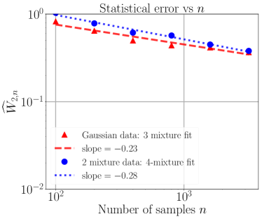
We now present several experiments that provide numerical backing to the claim that the slow rate of order $n^{-\frac{1}{4}}$ is not merely an artifact of the special balanced fit ((3) with $\uppi=\frac{1}{2}$). We demonstrate that the slow convergence of EM is very likely to arise while fitting general over-specified location Gaussian mixtures with unknown weights (and known covariance). We consider three settings: (A) fitting several general over-specified location Gaussian mixture fits to Gaussian data (Figure 7), (B) fitting a special three-component mixture fit to a two mixture of Gaussians (Figure 8), and (C) fitting mixtures with unknown weights and location parameters when the number of components in the fitted model is over-specified by two (Figure  9). We now turn to the details of these settings.

General over-specified mixture fits on Gaussian data

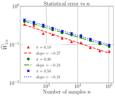
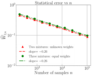
First, we remark that the fast convergence in the unbalanced fit (Theorem 1) was a joint result of the facts that (a) the weights were fixed and unequal, and (b) the parameters were constrained to be a sign flip. If either of these conditions is violated, the EM algorithm exhibits slow convergence on both algorithmic and statistical fronts. Theorems 2, 3 and 4 provide rigorous details for the case of equal and fixed weights (balanced fit). When the weights are unknown, EM can exhibit slow rate (see Section 5.1 and Appendix C.2 for further details). When the weights are fixed and unequal, but the location parameters are estimated freely—that is, with the model $\uppi\phi(x;\theta_{1},1)+(1-\uppi)\phi(x;\theta_{2},1)$, as illustrated in Figure 7(a)—then the EM estimates have error of order $n^{-\frac{1}{4}}$. In such cases, the parameter estimates approximately satisfy the relation $\sum_{k}\uppi_{k}\widehat{\theta}_{k,n}\approx 0$, since the mean of the data is close to zero; moreover, for a two-components mixture model, the location estimates become weighted sign flips of each other. The features are the intuitive reason underlying the similarity of behavior of EM between this fit and the balanced fit. Finally, when we fit a two mixture model with unknown weight parameter and free location parameters, the final error also has a scaling of order $n^{-\frac{1}{4}}$. Refer to Figure 7 for a numerical validation of these results.

(a)	(b)

Figure 7: Plots of the Wasserstein error $\widehat{W}_{2,n}$ associated with EM fixed points versus the sample size for fitting various kinds of location mixture models to standard normal $\mathcal{N}(0,1)$ data. We fit mixture models with either two or three components, with all location parameters estimated in an unconstrained manner. The lines are obtained by a linear regression of the log error on the sample size $n$. (a) Fitting a two-mixture model $\uppi\mathcal{N}(\theta_{1},1)+(1-\uppi)\mathcal{N}(\theta_{2},1)$ with three different fixed values of weights $\uppi\in\left\{0.1,0.3,0.5\right\}$ and two (unconstrained) location parameters, along with least-squares fits to the log errors. (b) Data plotted as red triangles is obtained by fitting a two-component model with unknown mixture weights and two location parameters $\uppi\mathcal{N}(\theta_{1},1)+(1-\uppi)\mathcal{N}(\theta_{2},1)$, whereas green circles correspond to results fitting a three-component mixture model $\sum_{i=1}^{3}\frac{1}{3}\mathcal{N}(\theta_{i},1)$. In all cases, the EM solutions exhibit the slow $n^{-\frac{1}{4}}$ statistical rate for the error in parameter estimation. Also see Figure 9.

Over-specified fits for mixtures of Gaussian data

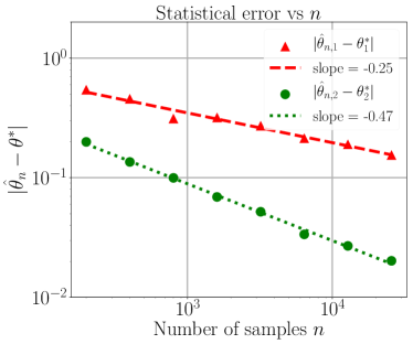
Using similar reasoning as above, let us sketch out how our theoretical results also yield usable predictions for more general over-specified models. Roughly speaking, whenever there are extra number of components to be estimated, parameters of some of them are likely to end up satisfying certain form of local constraint. More concretely, suppose that we are given data generated from a $k$-component mixture, and we use the EM algorithm to fit the location parameters of a mixture model with $k+1$ components. Loosely speaking, the EM estimates corresponding to a set of $k-1$ components are likely to converge quickly, leaving the two remaining components to fit a single component in the true model. If the other components are far away, the EM updates for the parameters of these two components are unaffected by them and start to behave like the balanced case. See Figure 8 for a numerical illustration of this intuition in an idealized setting where we use $k+1=3$ components to fit data generated from a $k=2$ component model. In this idealized setting, the error for one of the parameter scales at the fast rate of order $n^{-\frac{1}{2}}$, and that of the parameter that is locally over-fitted exhibits a slow rate of order $n^{-\frac{1}{4}}$. Finally, we see that the statistical error of order $n^{-\frac{1}{4}}$ also arises when we over-specify the number of components by more than one. In particular, we observe in Figure 7(b) (green dashed dotted line with solid circles) and Figure 9 (both curves) that a similar scaling of order $n^{-\frac{1}{4}}$ arises when we over-specify the number of components by $2$ and estimate the weight and location parameters.

Besides formally analyzing EM in these general cases, several other future directions arise from our work which we now discuss.

(a)	(b)

Figure 8: Behavior of EM for an over-specified Gaussian mixture. True model: $\frac{1}{2}\mathcal{N}(\theta^{*}_{1},1)+\frac{1}{2}\mathcal{N}(\theta^{*}_{2},1)$ where $\theta^{*}_{1}=0$ and $\theta^{*}_{2}=10$. We fit a model $\frac{1}{4}\mathcal{N}(-\theta_{1},1)+\frac{1}{4}\mathcal{N}(\theta_{1},1)+\frac{1}{2}\mathcal{N}(\theta_{2},1)$, where we initialize $\theta_{1}^{0}$ close to $\theta^{*}_{1}$ and $\theta_{2}^{0}$ close to $\theta^{*}_{2}$. (a) Population EM updates: We observe that while $\theta_{1}^{t}$ converges slowly to $\theta^{*}_{1}=0$, the iterates $\theta_{2}^{t}$ converge exponentially fast to $\theta^{*}_{2}=10$. (b) We plot the statistical error for the two parameters. While the strong signal component has a parametric $n^{-\frac{1}{2}}$ rate, for the no signal component EM has the slower $n^{-\frac{1}{4}}$ rate, which is in good agreement with the theoretical results derived in the paper. (We remark that the error floor for $\theta_{2}^{t}$ in panel (a) arises from the finite precision inherent to numerical integration.)

Figure 9: Plots of Wasserstein error when both weights and location parameters are unknown and estimated using EM and the fitted multivariate mixture model is over-specified. (a) True model: $\mathcal{N}([0,0]^{\top},I_{2})$, and fitted model $\sum_{i=1}^{3}w_{i}\mathcal{N}(\theta_{i},I_{2})$ and (b) True model: $\frac{2}{5}\mathcal{N}([0,0]^{\top},I_{2})+\frac{3}{5}\mathcal{N}([4,4]^{\top},I_{2})$ and fitted model: $\sum_{i=1}^{4}w_{i}\mathcal{N}(\theta_{i},I_{2})$. In both cases, once again we see the scaling of order $n^{-\frac{1}{4}}$ for the final error (similar to results in Figure 7 and 8).

5.4 Future directions

In our current work, we assumed that only the location parameters were unknown and that the scale parameters of the underlying model are known. Nevertheless in practice, this assumption is rather restrictive and it is natural to ask what happens if the scale parameters were also unknown. We note that the MLE is known to have even slower statistical rates for the estimation error with such higher-order mixtures; therefore, it would be interesting to determine if the EM algorithm also suffers from a similar slow down when the scale parameters are unknown. We refer the readers to a recent preprint [10], where we establish that the EM algorithm can suffer from a further slow-down on the statistical and computational ends when over-specified mixtures are fitted with an unknown scale parameter.

Another important direction is to analyze the behavior of EM under different models for generating the data. While our analysis is focused on Gaussian mixtures, the non-standard statistical rate $n^{-\frac{1}{4}}$ also arises in other types of over-specified mixture models, such as those involving mixtures with other exponential family members, or Student-$t$ distributions, suitable for heavy-tailed data. We believe that the analysis of our paper can be generalized to a broader class of finite mixture models that includes the aforementioned models.

A final direction of interest is whether the behavior of EM—slow versus fast convergence—can be used as a statistic in a classical testing problem: testing the simple null of a standard multivariate Gaussian versus the compound alternative of a two-component Gaussian mixture. This problem is known to be challenging due to the break-down of the (generalized) likelihood ratio test, due the singularity of the Fisher information matrix; see the papers [21, 6] for some past work on the problem. The results of our paper suggest an alternative approach, which is based on monitoring the convergence rate of EM. If the EM algorithm converges slowly for a balanced fit, then we may accept the null, whereas the opposite behavior can be used as an evidence for rejecting the null. We leave for future work the analysis of such a testing procedure based on the convergence rates of EM.

Appendix A Proofs of main results

In this appendix, we present the proofs of our main results, namely Theorems 1, 2, 3, and 4.

A.1 Proof of Theorem 1

As alluded to earlier in Section 3.1—given Lemma 1—it suffices to prove the contraction property (10a) for the population operator $M$. Recall that $\theta^{*}=0$ is a fixed point of the population EM operator (i.e., $M(0)=0$). This fact, combined with the definition (8) of the M-update, yields

$$\left\|M(\theta)\right\|_{2}=\left\|M(\theta)-M(\theta^{*})\right\|_{2}=\left\|{\mathbb{E}}\left[2(w_{\theta}(X)-w_{0}(X))X\right]\right\|_{2},$$

where, in the unbalanced setting (3), the weight function $w_{\theta}$ (6) and the gradient $\nabla_{\theta}w_{\theta}$ take the form

$$w_{\theta}(X) =\frac{\uppi}{\uppi+(1-\uppi)e^{-\frac{2\theta^{\top}X}{\sigma^{2}}}},\ \mbox{and}\ \nabla_{\theta}w_{\theta}(X)=\frac{\frac{2\uppi(1-\uppi)X}{\sigma^{2}}}{\left(\uppi e^{-\frac{\theta^{\top}X}{\sigma^{2}}}+(1-\uppi)e^{\frac{\theta^{\top}X}{\sigma^{2}}}\right)^{2}}.$$

For a scalar $u\in[0,1]$, define the function $h(u)=w_{u\theta}(X)$, and note that $h^{\prime}(u)=\nabla w_{u\theta}(X)^{\top}\theta$. Thus, using a Taylor series expansion along the line $\theta_{u}=u\theta,u\in[0,1]$, we find that

$$\left\|M(\theta)\right\|_{2} =\left\|{\mathbb{E}}\left[2X\int_{0}^{1}h^{\prime}(u)du\right]\right\|_{2}$$

$$=4\uppi(1-\uppi)\left\|\int\limits_{0}^{1}{\mathbb{E}}\left[\frac{XX^{\top}}{\sigma^{2}\left(\uppi\exp\left(-\frac{\theta_{u}^{\top}X}{\sigma^{2}}\right)+(1-\uppi)\exp\left(\frac{\theta_{u}^{\top}X}{\sigma^{2}}\right)\right)^{2}}\right]\theta du\right\|_{2}$$

$$\leq 4\uppi(1-\uppi)\|\theta\|_{2}\max\limits_{u\in[0,1]}|\!|\!|{\mathbb{E}}\left[\Gamma_{\theta_{u}}(X)\right]|\!|\!|_{{\tiny{\mbox{op}}}},$$ (27)

where in the last equation we have defined the matrix

$$\Gamma_{\theta_{u}}(X):=\frac{XX^{\top}}{\sigma^{2}\left(\uppi\exp\left(-\frac{\theta_{u}^{\top}X}{\sigma^{2}}\right)+(1-\uppi)\exp\left(\frac{\theta_{u}^{\top}X}{\sigma^{2}}\right)\right)^{2}}.$$ (28)

Writing the mixture weight as $\uppi=\frac{1}{2}\left(1-\rho\right)$, we claim that it suffices to show that

$$\max\limits_{u\in[0,1]}|\!|\!|{\mathbb{E}}\left[\Gamma_{\theta_{u}}(X)\right]|\!|\!|_{{\tiny{\mbox{op}}}} \leq\frac{1-\rho^{2}/2}{1-\rho^{2}}.$$ (29)

Indeed, taking the last bound as given and substituting it into inequality (27), we find that

$$\left\|M(\theta)\right\|_{2} \leq 4\uppi\,(1-\uppi)\,\frac{1-\rho^{2}/2}{1-\rho^{2}}\;\left\|\theta\right\|_{2}\;=\;(1-\rho^{2}/2)\left\|\theta\right\|_{2},$$

which yields the claim (10a) of Theorem 1.

Proof of claim (29)

We begin by making a convenient change of coordinates. Let $R\in{}^{d\times d}$ be an orthonormal matrix such that $R\theta_{u}=\left\|\theta_{u}\right\|_{2}e_{1}$, where $e_{1}$ denotes the first canonical basis vector in dimension $d$. Define the random vector $V:=RX/\sigma$. Since the vector $X\sim\mathcal{N}(0,\sigma^{2}I_{d})$ and the matrix $R$ is orthonormal, the random vector $V$ follows a $\mathcal{N}(0,I_{d})$ distribution. Substituting $X=\sigma R^{\top}V$ and $R\theta_{u}=\left\|\theta_{u}\right\|_{2}e_{1}$ in the expression (28) for $\Gamma_{\theta_{u}}$ and using the fact that $|\!|\!|R^{\top}BR|\!|\!|_{{\tiny{\mbox{op}}}}=|\!|\!|B|\!|\!|_{{\tiny{\mbox{op}}}}$ for any matrix $B$ and any orthogonal matrix $R$, we find that $|\!|\!|{\mathbb{E}}\left[\Gamma_{\theta_{u}}(X)\right]|\!|\!|_{{\tiny{\mbox{op}}}}=|\!|\!|B_{\theta_{u}}|\!|\!|_{{\tiny{\mbox{op}}}}$, where

$$B_{\theta_{u}}:={\mathbb{E}}_{V}\left[\frac{VV^{\top}}{\left(\uppi\exp\left(-\left\|\theta_{u}\right\|_{2}V_{1}/\sigma\right)+(1-\uppi)\exp\left(\left\|\theta_{u}\right\|_{2}V_{1}/\sigma\right)\right)^{2}}\right].$$

Here $V_{1}:=Ve_{1}$ denotes the first coordinate of the random vector $V$. Note that the matrix $B_{\theta_{u}}$ is a diagonal matrix, with non-negative entries. Thus, in order to prove the bound (29), it suffices to show that

$$\max_{j\in[d]}[B_{\theta_{u}}]_{jj}\leq\frac{1-\rho^{2}/2}{1-\rho^{2}}.$$ (30)

When $\theta_{u}=0$, the matrix $B_{\theta_{u}}={\mathbb{E}}[VV^{\top}]=I_{d}$ and the claim holds trivially. Turning to the case $\theta_{u}\neq 0$, we split our analysis into two cases, depending on whether $j=1$ or $j\neq 1$.

Bounding $[B_{\theta_{u}}]_{11}$

Denoting $\uppi=\frac{1}{2}(1-\rho)$, we observe that

$$(\uppi e^{-y}+(1-\uppi)e^{y}) \in[\sqrt{(1-\rho^{2})},\,1],\quad\text{ if }e^{y}\in\left[1,\frac{1+\rho}{1-\rho}\right],\quad\text{and}$$

$$(\uppi e^{-y}+(1-\uppi)e^{y}) >1,\quad\quad\quad\quad\quad\quad\quad\text{otherwise}.$$ (31)

Let $\mathcal{E}^{c}$ and $\mathbb{I}(\mathcal{E})$ respectively denote the complement and the indicator of any event $\mathcal{E}$. Define the event

$$\mathcal{E}_{\theta_{u}}:=\left\{e^{\left\|\theta_{u}\right\|_{2}V_{1}/\sigma}\in\left[1,\frac{1+\rho}{1-\rho}\right]\right\}.$$

Using the observation (31) above and the fact that $V_{1}\sim\mathcal{N}(0,1)$, we obtain

$$[B_{\theta_{u}}]_{11} ={\mathbb{E}}\left[\frac{V_{1}^{2}}{\left(\uppi\exp\left(-\left\|\theta_{u}\right\|_{2}V_{1}/\sigma\right)+(1-\uppi)\exp\left(\left\|\theta_{u}\right\|_{2}V_{1}/\sigma\right)\right)^{2}}\right]$$

$$\leq\frac{1}{(1-\rho^{2})}{\mathbb{E}}\left[V_{1}^{2}\,\mathbb{I}(\mathcal{E}_{\theta_{u}})\right]+{\mathbb{E}}\left[V_{1}^{2}\,\mathbb{I}(\mathcal{E}_{\theta_{u}}^{c})\right]$$

$$=\frac{1-\rho^{2}+\rho^{2}{\mathbb{E}}\left[V_{1}^{2}\,\mathbb{I}(\mathcal{E}_{\theta_{u}})\right]}{(1-\rho^{2})}.$$ (32)

Note that whenever $\theta_{u}\neq 0$, we have that $\mathcal{E}_{\theta_{u}}\subseteq\big{\{}V_{1}\geq 0\}$ and consequently, we obtain that

$${\mathbb{E}}\left[V_{1}^{2}\,\mathbb{I}(\mathcal{E}_{\theta_{u}})\right]\leq{\mathbb{E}}\left[V_{1}^{2}\,\mathbb{I}(V_{1}\geq 0)\right]=\frac{1}{2}.$$ (33)

Putting the inequalities (32) and (33) together, we conclude that
$[B_{\theta_{u}}]_{11}\leq({1-\rho^{2}/2})/({1-\rho^{2}})$.

Bounding $[B_{\theta_{u}}]_{jj},\;j\neq 1$

Using arguments similar to the previous case, and the fact that the random variables $V_{i},i\in[d]$, are independent standard normal random variables, we find that

$$[B_{\theta_{u}}]_{jj} ={\mathbb{E}}\left[\frac{V_{j}^{2}}{\left(\uppi\exp\left(-\left\|\theta_{u}\right\|_{2}V_{1}/\sigma\right)+(1-\uppi)\exp\left(\left\|\theta_{u}\right\|_{2}V_{1}/\sigma\right)\right)^{2}}\right]$$

$$={\mathbb{E}}\left[\frac{1}{\left(\uppi\exp\left(-\left\|\theta_{u}\right\|_{2}V_{1}/\sigma\right)+(1-\uppi)\exp\left(\left\|\theta_{u}\right\|_{2}V_{1}/\sigma\right)\right)^{2}}\right].$$

Invoking the definition of the event $\mathcal{E}_{\theta_{u}}$, we have

$$[B_{\theta_{u}}]_{jj} \leq\frac{1}{(1-\rho^{2})}{\mathbb{E}}\left[\mathbb{I}(\mathcal{E}_{\theta_{u}})\right]+{\mathbb{E}}\left[\mathbb{I}(\mathcal{E}_{\theta_{u}}^{c})\right]=\frac{1-\rho^{2}+\rho^{2}{\mathbb{E}}\left[\mathbb{I}(\mathcal{E}_{\theta_{u}})\right]}{(1-\rho^{2})}.$$

Finally, noting that ${\mathbb{E}}\left[\mathbb{I}(\mathcal{E}_{\theta_{u}})\right]\leq{\mathbb{E}}\left[\mathbb{I}(V_{1}\geq 0)\right]=1/2$ whenever $\theta_{u}\neq 0$, yields the claim.

A.2 Proof of Theorem 2

We split our proof into two parts, which correspond to the upper bound (13a) and the lower bound (13b) respectively.

A.2.1 Proof of the upper bound (13a)

For the balanced fit, we have

$$w_{\theta}(X)=\dfrac{1}{1+e^{-2\theta^{\top}X/\sigma^{2}}}\quad\mbox{and}\quad\nabla_{\theta}(w_{\theta}(X))=\dfrac{2X^{\top}/\sigma^{2}}{(e^{-\theta^{\top}X/\sigma^{2}}+e^{\theta^{\top}X/\sigma^{2}})^{2}}.$$

Using a Taylor expansion and repeating the preliminary computations as those in the proof of Theorem 1 from the unbalanced setting, we obtain that

$$\left\|M(\theta)\right\|_{2} =\left\|{\mathbb{E}}\left[2X\int_{0}^{1}w^{\prime}_{\theta_{u}}(X)^{\top}\theta_{u}du\right]\right\|_{2}$$

$$=4\bigg{\|}\int\limits_{0}^{1}{\mathbb{E}}\left[\frac{XX^{\top}}{\sigma^{2}\left(e^{-\theta_{u}^{\top}X/\sigma^{2}}+e^{\theta_{u}^{\top}X/\sigma^{2}}\right)^{2}}\right]\theta du\bigg{\|}_{2}$$ (34)

$$\leq 4\left\|\theta\right\|_{2}\int\limits_{0}^{1}|\!|\!|{\mathbb{E}}\left[\Gamma_{\theta_{u}}(X)\right]|\!|\!|_{{\tiny{\mbox{op}}}}du,$$

where $\Gamma_{\theta_{u}}(X):=\frac{XX^{\top}/\sigma^{2}}{(e^{-\theta_{u}^{\top}X/\sigma^{2}}+e^{\theta_{u}^{\top}X/\sigma^{2}})^{2}}$. Consequently, in order to prove the upper bound (13a), it suffices to show that

$$\int_{0}^{1}|\!|\!|{\mathbb{E}}\left[\Gamma_{\theta_{u}}(X)\right]|\!|\!|_{{\tiny{\mbox{op}}}}du\leq\frac{1}{4}\left(p+\frac{1-p}{1+\left\|\theta\right\|_{2}^{2}/2\sigma^{2}}\right)=\frac{\gamma_{\textrm{up}}(\theta)}{4}$$ (35)

where $p:=(1+{\mathbb{P}}_{Z\sim\mathcal{N}(0,1)}(\left|Z\right|\leq 1))/2<1$.

We now establish the claim (35). Like in proof of Theorem 1, we perform a change of coordinates using an orthogonal matrix $R$ such that $R\theta_{u}=\left\|\theta_{u}\right\|_{2}e_{1}$, where $e_{1}$ is the first canonical basis in dimension $d$. Define the random vector $V:=RX/\sigma$. Since the vector ${X\sim\mathcal{N}(0,\sigma^{2}I_{d})}$ and the matrix $R$ is orthogonal, we have that the vector ${V\sim\mathcal{N}(0,I_{d})}$. Substituting the matrix $X=\sigma R^{\top}V$ and ${R\theta_{u}=\left\|\theta_{u}\right\|_{2}e_{1}}$ in the expression for $\Gamma_{\theta_{u}}$ and using the equality $|\!|\!|R^{\top}BR|\!|\!|_{{\tiny{\mbox{op}}}}=|\!|\!|B|\!|\!|_{{\tiny{\mbox{op}}}}$, valid for any matrix $B$ and any orthogonal matrix $R$, we obtain that $|\!|\!|{\mathbb{E}}\left[\Gamma_{\theta_{u}}(X)\right]|\!|\!|_{{\tiny{\mbox{op}}}}=|\!|\!|B_{\theta_{u}}|\!|\!|_{{\tiny{\mbox{op}}}}$, where

$$B_{\theta_{u}}:={\mathbb{E}}_{V}\left[\frac{VV^{\top}}{\left(\exp\left(-\left\|\theta_{u}\right\|_{2}V_{1}/\sigma\right)+\exp\left(\left\|\theta_{u}\right\|_{2}V_{1}/\sigma\right)\right)^{2}}\right].$$ (36)

Clearly, the matrix $B_{\theta_{u}}$ is a diagonal matrix with non-negative entries (note the abuse of notation: the definitions of the matrices $\Gamma_{\theta_{u}}$ and $B_{\theta_{u}}$ is different from the unbalanced case). Consequently, to obtain a bound for the operator norm of the matrix $B_{\theta_{u}}$, it is sufficient to provide an upper bound on the diagonal entries of the matrix $B_{\theta_{u}}$. In order to do so, we introduce an auxiliary claim:

Lemma 2.

The $\ell_{2}$-operator norm of the matrix $B_{\theta_{u}}$ defined in equation (36), is upper-bounded as

$$|\!|\!|B_{\theta_{u}}|\!|\!|_{{\tiny{\mbox{op}}}}=\max_{j\in[d]}[B_{\theta_{u}}]_{jj}\leq\frac{p_{2}}{4}+\frac{(1-p_{2})}{4}\frac{1}{(1+\left\|\theta_{u}\right\|_{2}^{2}/(2\sigma^{2}))^{2}},$$ (37)

where $p_{2}={\mathbb{P}}\left(|V_{1}|\leq 1\right)<1$.

See Appendix B.2 for the proof of Lemma 2.

Using Lemma 2, we now complete the proof. Integrating both sides of the inequality (37) with respect to $u\in[0,1]$, we find that

$$\int_{0}^{1}|\!|\!|B_{\theta_{u}}|\!|\!|_{{\tiny{\mbox{op}}}}du \leq\int_{0}^{1}\frac{p_{2}}{4}du+\int_{0}^{1}\frac{(1-p_{2})}{4}\frac{1}{(1+\left\|\theta_{u}\right\|_{2}^{2}/(2\sigma^{2}))^{2}}du$$

$$=\frac{p_{2}}{4}+\frac{(1-p_{2})}{4}\int_{0}^{1}\frac{1}{(1+u^{2}\left\|\theta\right\|_{2}^{2}/(2\sigma^{2}))^{2}}du.$$

Direct computation of the second integral yields

$$\int\limits_{0}^{1}\frac{1}{(1+u^{2}\left\|\theta\right\|_{2}^{2}/(2\sigma^{2}))^{2}}du =\dfrac{1}{2}\biggr{(}\frac{1}{1+\frac{\|\theta\|^{2}}{2\sigma^{2}}}+\frac{\tan^{-1}(\|\theta\|/(\sqrt{2}\sigma)}{\|\theta\|/(\sqrt{2}\sigma)}\biggr{)}$$

$$\leq\dfrac{1}{2}\biggr{(}\frac{1}{1+\frac{\|\theta\|^{2}}{2\sigma^{2}}}+1\biggr{)},$$

where the last inequality above follows since $\tan^{-1}(y)\leq y$, for all $y\geq 0$. Putting together the pieces yields

$$\int_{0}^{1}|\!|\!|{\mathbb{E}}\left[\Gamma_{\theta_{u}}(X)\right]|\!|\!|_{{\tiny{\mbox{op}}}}du=\int_{0}^{1}|\!|\!|B_{\theta_{u}}|\!|\!|_{{\tiny{\mbox{op}}}}du\leq\frac{(1+p_{2})}{8}+\frac{(1-p_{2})/8}{1+\left\|\theta\right\|_{2}^{2}/(2\sigma^{2})},$$

which implies the claim (35) with $p=\frac{1+p_{2}}{2}$.

A.2.2 Proof of the lower bound (13b)

We now prove the lower bound (13b) of Theorem 2 on the population EM operator $M$. The argument involves Jensen’s inequality and certain properties of the moment generating function (MGF) of the Gaussian distribution.

Recalling equation (34), we find that

$$\left\|M(\theta)\right\|_{2} =4\bigg{\|}\underbrace{\int\limits_{0}^{1}{\mathbb{E}}\bigg{[}{\frac{XX^{\top}}{\sigma^{2}\left(\exp\left(-{\theta_{u}^{\top}X}/{\sigma^{2}}\right)+\exp\left({\theta_{u}^{\top}X}/{\sigma^{2}}\right)\right)^{2}}}\bigg{]}du}_{=:\Gamma_{\theta}}\,\,\theta\bigg{\|}_{2}$$

$$\geq 4\lambda_{\min}\left(\Gamma_{\theta}\right)\left\|\theta\right\|_{2},$$ (38)

where $\lambda_{\min}(\Gamma_{\theta})$ denotes the smallest eigenvalue of the square matrix $\Gamma_{\theta}$. Following the change of variable $V:=RX/\sigma$ used in the proof of upper bound (13a), we obtain that

$$\lambda_{\min}\left(\Gamma_{\theta}\right)=\lambda_{\min}\bigg{(}\underbrace{{\mathbb{E}}_{V}\bigg{[}\int\limits_{0}^{1}\frac{VV^{\top}}{\left(\exp\left(-\|\theta_{u}\|_{2}V_{1}/\sigma\right)+\exp\left(\|\theta_{u}\|_{2}V_{1}/\sigma\right)\right)^{2}}du\bigg{]}}_{=:F_{\theta}}\bigg{)}.$$ (39)

Clearly, the matrix $F_{\theta}$ is a diagonal matrix with non-negative diagonal entries and consequently, we have

$$\lambda_{\min}(F_{\theta})=\min_{j\in[d]}[F_{\theta}]_{jj}.$$ (40)

In order to provide a lower bound on the diagonal entries of the matrix $F_{\theta}$, we use the following auxiliary claim:

Lemma 3.

For all vectors $\theta\in{}^{d}$ such that $\left\|\theta\right\|_{2}^{2}\leq\frac{5\sigma^{2}}{8}$, the matrix $F_{\theta}$ defined in equation (39), satisfies the bounds

$$\left[F_{\theta}\right]_{jj}\geq\left[F_{\theta}\right]_{11}\geq\frac{1}{4(1+{2\left\|\theta\right\|_{2}^{2}}/{\sigma^{2}})}\quad\text{for all $j\in[d]$.}$$ (41)

See Appendix B.3 for the proof of this claim.

Finally, combining the result of Lemma 3 with equations (38) and (40), we conclude that

$$\frac{\left\|M(\theta)\right\|_{2}}{\left\|\theta\right\|_{2}} \geq 4\lambda_{\min}\left(\Gamma_{\theta}\right)\;=\;4[F_{\theta}]_{11}\;\geq\;\frac{1}{({1+2\left\|\theta\right\|_{2}^{2}/\sigma^{2}})}=\gamma_{\textrm{low}}(\theta),$$

as claimed.

A.3 Proof of Theorem 3

The reader should recall the framework that was laid out in Section 4.1, especially Lemma 1 which was used to bound the deviation between the sample and population EM operators, as well the annulus-based localization argument (that breaks up the iterations of EM into different epochs) sketched out in Section 4.2. The proof of Theorem 3 is based on making this proof outline more precise.

A.3.1 Epochs and non-expansivity

Let us introduce the notation required to formalize the analysis that leads to the recursion (23). Recall that the recursion (23) generates the sequence $\{\alpha_{\ell}\}_{\ell\geq 0}$ given by

$$\alpha_{0}=0\quad\text{and}\quad\alpha_{\ell+1}=\frac{\alpha_{\ell}}{3}+\frac{1}{6},\quad\mbox{for $\ell=0,1,2,\ldots$.}$$ (42a)

By inspection, this sequence is increasing and satisfies $$\lim\limits_{\ell\to\infty}\alpha_{\ell}=1/4 \alpha_{\ell}\leq 1/4-\epsilon \ell\geq\lceil\log(4/\epsilon)/\log 3\rceil \delta\in(0,1)$$. Furthermore, we have for . For any given , define the following intermediate quantity

$$\omega=\sigma^{2}\left(\frac{d+\log((2\ell_{\epsilon}+1)/\delta)}{n}\right)\text{ where }\ell_{\epsilon}:=\lceil\log(4/\epsilon)/\log 3\rceil+1.$$ (42b)

Note that the lower bound on the sample size stated in the theorem ensures that $$\omega\leq 1 \omega\approx d/n (n,d)$$. For the proof sketch provided in Section 4.2, we used the rough approximation , which is adequate when tracking only the dependency on the pair .

For $\ell=0,1,2,\ldots,\ell_{\epsilon}-1$, define the scalars $t_{\ell}$ and $T_{\ell}$ as

$$t_{0}=\left\lceil\frac{2}{p}\log\frac{\left\|\theta_{0}\right\|_{2}}{\sqrt{2}\sigma\sqrt{\omega}}\right\rceil,\ \ t_{\ell}=\left\lceil\frac{2}{p\omega^{2\alpha_{\ell+1}}}\log(1/\omega)\right\rceil,\ \text{ and}\ T_{\ell}=\sum_{j=0}^{\ell}t_{j},$$ (42c)

where $\lceil y\rceil$ denotes the smallest integer greater than or equal to $y$, and the constant $p\in(0,1)$ is given by $p={\mathbb{P}}(\left|X\right|\leq 1)+\frac{1}{2}{\mathbb{P}}(\left|X\right|>1)$ where $X\sim\mathcal{N}(0,1)$. For each $\ell=1,2,\ldots$, the term $t_{\ell}$ corresponds to the number of iterations for the $\ell$-th epoch, whereas the quantity $T_{\ell}$ denotes the total number of iterations up to the completion of that epoch.

Recall that Lemma 1, stated in the main paper, gives us a bound on $\sup_{\|\theta\|_{2}\leq r}\left\|M_{n}(\theta)-M(\theta)\right\|_{2}$ for a given radius $r$. In the epoch-based argument, we have a sequence of such radii (corresponding to the outer radii of the annulus considered in each epoch), so that we need to control this same quantity uniformly over all radii $r$ in the set $\mathcal{R}$ given by

$$\mathcal{R} =\left\{\left\|\theta^{0}\right\|_{2},\sqrt{2}\sigma\omega^{\alpha_{0}},\ldots,\sqrt{2}\sigma\omega^{\alpha_{\ell_{\epsilon}-1}},c^{\prime}\sqrt{2}\sigma\omega^{\alpha_{0}},\ldots,c^{\prime}\sqrt{2}\sigma\omega^{\alpha_{\ell_{\epsilon}-1}}\right\}.$$ (43)

Here ${c^{\prime}=(2c_{1}\sigma/p+1)}$ denotes a constant independent of $n,d,\delta$ and $\epsilon$ where $c_{1}$ is the universal constant that appeared in the bound from Lemma 1. In order to do so, we apply a standard union bound with Lemma 1 and obtain that

$$\sup_{\|\theta\|_{2}\leq r}\left\|M_{n}(\theta)-M(\theta)\right\|_{2}\leq c_{1}\sigma r\sqrt{\omega}\quad\text{ for all }r\in\mathcal{R},$$ (44)

with probability at least $1-\delta$. Let $\mathcal{E}(n,d,\epsilon,\delta)$ denote the event that the bound (44) holds.

With this notation in place, we start with our first claim. The sample-based EM operator is non-expansive in the following sense:

Lemma 4.

Consider the sample-based EM iteration $\theta^{t+1}=M_{n}(\theta^{t})$ with a sample size $n\geq(2c_{1}\sigma/p)^{1/(2\epsilon)}\sigma^{2}(d+\log((2\ell_{\epsilon}+1)/\delta))$. Suppose that there exists an index $\ell\in\left\{0,1,\ldots,\ell_{\epsilon}-1\right\}$ and an iteration number $t$ such that $\left\|\theta^{t}\right\|_{2}\leq\sqrt{2}\sigma\omega^{\alpha_{\ell}}$. Then, conditional on the event $\mathcal{E}(n,d,\epsilon,\delta)$ from equation (44), we have

$$\|{\theta^{t^{\prime}}}\|_{2}\leq\sqrt{2}\sigma\omega^{\alpha_{\ell}}\qquad\mbox{for all $t^{\prime}\geq t$.}$$ (45)

See Appendix B.4 for the proof of this claim.

A.3.2 Core of the argument

We now proceed to the core of the argument. Suppose that the sample size is lower bounded as

$$n\geq\max\left\{c_{2},\left(\frac{2c_{1}\sigma}{p}+1\right)^{\frac{4}{\epsilon}},\left(\frac{\sqrt{2}c_{1}\left\|\theta^{0}\right\|_{2}}{p}+1\right)^{2}\right\}\cdot\sigma^{2}(d+\log\left(\frac{3\log(4/\epsilon)}{\delta}\right)),$$ (46)

where the constants $c_{1}$ and $c_{2}$ correspond to that from Lemma 1. Moreover, recall that the quantity $\omega$ and the time-steps $T_{\ell}$ were defined in equations (42b) and (42c) respectively. The core of the proof consists of the following:

Key claim

For all $\ell\in\left\{0,1,\ldots,\ell_{\epsilon}-1\right\}$, we have

$$\left\|\theta^{t}\right\|_{2} \leq\sqrt{2}\sigma\omega^{\alpha_{\ell}}\qquad\text{ for all }t\geq T_{\ell},$$ (47)

with probability at least $1-\delta$.

Taking this claim as given, let us now show how the bounds in Theorem 3 hold for all $t\geq T_{\ell_{\epsilon}-1}$. Straightforward computations yield that

$$T_{\ell_{\epsilon}-1} \leq T_{0}+(\ell_{\epsilon}-1)t_{\ell_{\epsilon}-1}$$

$$\leq\frac{4}{p}\left[\log\frac{\left\|\theta_{0}\right\|_{2}}{\sqrt{2}\sigma\sqrt{\omega}}+\log\frac{4}{\epsilon}\cdot\omega^{1/2-2\epsilon}\cdot\log\frac{n}{\sigma^{2}d}\right]$$

$$\leq\frac{8}{p}\left[\log\frac{\left\|\theta_{0}\right\|_{2}^{2}n}{\sigma^{2}d}+\left(\frac{n}{d}\right)^{\frac{1}{2}-2\epsilon}\cdot\log\left(\frac{4}{\epsilon}\right)\cdot\log\left(\frac{n}{\sigma^{2}d}\right)\cdot\sigma^{4\epsilon-1}\right].$$ (48)

In other words, equations (46) and (48) provide the explicit expression for the number of samples and number of steps required by sample-based EM to converge to a ball of radius $(d/n)^{1/4-\epsilon}$ around the truth $\theta^{*}=0$.

Proof of the claim (47)

It remains to prove the key claim, and we do so by an induction on the epoch index $\ell$. All of the argument are performed conditioned on the event $\mathcal{E}(n,d,\epsilon,\delta)$ defined in equation (44); note that this event occurs with probability at least $1-\delta$. Moreover, we see that the sample size assumption (46) for Theorem 3 is larger than required in Lemma 4 and hence we can invoke the non-expansiveness of the sample-based EM operator in our arguments to follow.

Proof of base case: ($\ell=0$)

We adopt the shorthand $\nu=\left\|\theta_{0}\right\|_{2}/{\sqrt{2}\sigma}$. The non-expansiveness property of the sample-based EM-operator (Lemma 4) ensures that it is sufficient to consider the case that $\left\|\theta^{t}\right\|_{2}\in[\sqrt{2}\sigma,\nu\sqrt{2}\sigma]$ for all $t\leq T_{0}$. Applying the triangle inequality yields

$$\left\|\theta^{t+1}\right\|_{2} \leq\left\|M_{n}(\theta^{t})-M(\theta^{t})\right\|_{2}+\left\|M(\theta^{t})\right\|_{2}$$ (49a)

$$\stackrel{{\scriptstyle(i)}}{{\leq}}c_{1}\sigma\cdot\nu\sqrt{2}\sigma\cdot\sqrt{\omega}+\gamma_{\textrm{up}}(\theta^{t})\left\|\theta^{t}\right\|_{2},$$ (49b)

where step (i) follows from using $r=\nu\sqrt{2}\sigma$ in the event (44), and applying Theorem 2 (for the two terms respectively). Noting that $\left\|\theta^{t}\right\|_{2}\geq\sqrt{2}\sigma$, we also have that

$$\gamma_{\textrm{up}}(\theta^{t})=1-p+\frac{p}{1+\left\|\theta^{t}\right\|_{2}^{2}/\sigma^{2}}=1-\frac{p\left\|\theta^{t}\right\|_{2}^{2}}{\left\|\theta^{t}\right\|_{2}^{2}+2\sigma^{2}}\leq\underbrace{1-\frac{p}{2}}_{\overline{\gamma}_{0}}.$$

Recursing the inequalities (49a) and (49b) from $t=0$ up to $t=T_{0}$, and using the fact that $\gamma_{\textrm{up}}(\theta^{t})\leq\overline{\gamma}_{0}$, we find that

$$\left\|\theta^{T_{0}}\right\|_{2} \leq c_{1}\sigma\cdot\nu\sqrt{2}\sigma\cdot\sqrt{\omega}(1+\overline{\gamma}_{0}+\ldots+\overline{\gamma}_{0}^{T_{0}-1})+\overline{\gamma}_{0}^{T_{0}}\left\|\theta^{0}\right\|_{2}$$

$$\leq\frac{c_{1}\sigma\cdot\nu\sqrt{2}\sigma\cdot\sqrt{\omega}}{1-\overline{\gamma}_{0}}+\overline{\gamma}_{0}^{T_{0}}\nu\sqrt{2}\sigma.$$

Substituting the expressions $\overline{\gamma}_{0}=1-p/2$ and $T_{0}=\lceil(2/p)\log(\nu/\sqrt{\omega})\rceil$, we obtain that

$$\left\|\theta^{T_{0}}\right\|_{2}\leq\left(2\nu c_{1}\sigma/p+1\right)\sqrt{\omega}\sqrt{2}\sigma\leq\sqrt{2}\sigma,$$

where the last inequality follows from the fact that for the assumed bound (46) on $n$, we have $(2\nu c_{1}\sigma/p+1)\sqrt{\omega}\leq 1$. The base-case now follows.

Proof of inductive step

Now we prove the inductive step. In particular, we assume that $\left\|\theta^{T_{\ell}}\right\|_{2}\leq\sqrt{2}\sigma\omega^{\alpha_{\ell}}$ and show that $\left\|\theta^{T_{\ell+1}}\right\|_{2}\leq\sqrt{2}\sigma\omega^{\alpha_{\ell+1}}$. Once again, Lemma 4 implies that we may assume without loss of generality that $\left\|\theta^{t}\right\|_{2}\in[\omega^{\alpha_{\ell+1}},\omega^{\alpha_{\ell}}]$ for all $t\in\left\{T_{\ell},\ldots,T_{\ell+1}\right\}$. Under this condition, we have that

$$\gamma_{\textrm{up}}(\theta^{t})\leq 1-\frac{p\omega^{2\alpha_{\ell+1}}}{1+\omega^{2\alpha_{\ell+1}}}\leq\underbrace{1-\frac{p\omega^{2\alpha_{\ell+1}}}{2}}_{=:\overline{\gamma}_{\ell}}\quad\text{ for all }t\in\left\{T_{\ell},\ldots,T_{\ell+1}-1\right\},$$ (50)

where the last step follows from the fact that $\omega\in[0,1]$ and $\alpha_{\ell}\geq 0$. From our earlier definition (42c), we have $T_{\ell+1}=T_{\ell}+t_{\ell}$. We split the remainder of our proof in two parts, primarily to handle the constants. First, we show that

$$\left\|\theta^{T_{\ell}+\lceil t_{\ell+1}/2\rceil}\right\|_{2}\leq c^{\prime}\sqrt{2}\sigma\omega^{\alpha_{\ell+1}},$$ (51a)

where $$c^{\prime}=(2c_{1}\sigma/p+1) n,d,\delta \epsilon$$ is a constant independent of and . Next we use this result to show that

$$\left\|\theta^{T_{\ell+1}}\right\|_{2}=\left\|\theta^{T_{\ell}+t_{\ell+1}}\right\|_{2}\leq\sqrt{2}\sigma\omega^{\alpha_{\ell+1}},$$ (51b)

which completes the proof of the induction step. We now prove these two claims one by one.

Proof of claim (51a)

Applying the triangle inequality yields

$$\left\|\theta^{T_{\ell}+1}\right\|_{2} \leq\left\|M_{n}(\theta^{T_{\ell}})-M(\theta^{T_{\ell}})\right\|_{2}+\left\|M(\theta^{T_{\ell}})\right\|_{2}$$

$$\stackrel{{\scriptstyle(i)}}{{\leq}}c_{1}\sigma\cdot\sqrt{2}\sigma\omega^{\alpha_{\ell}}\cdot\sqrt{\omega}+\gamma_{\textrm{up}}(\theta^{T_{\ell}})\left\|\theta^{T_{\ell}}\right\|_{2},$$ (52)

where step (i) follows from using $r=\sqrt{2}\sigma\omega^{\alpha_{\ell}}$ in the event (44) and applying Theorem 2. Recursing the inequality (A.3.2) for $T\leq\lceil t_{\ell}/2\rceil$ steps, and invoking the bound (50), i.e., $\gamma_{\textrm{up}}(\theta^{t})\leq\overline{\gamma}_{\ell}$ for all $t\in\left\{T_{\ell},\ldots,T_{\ell}+T\right\}$, we obtain that

$$\left\|\theta^{T_{\ell}+T}\right\|_{2} \leq c_{1}\sigma\cdot\sqrt{2}\sigma\omega^{\alpha_{\ell}}\cdot\sqrt{\omega}\cdot(1+\overline{\gamma}_{\ell}+\ldots+\overline{\gamma}_{\ell}^{T-1})+\overline{\gamma}_{\ell}^{T}\left\|\theta^{T_{\ell}}\right\|_{2}$$

$$\leq\frac{c_{1}\sigma\cdot\sqrt{2}\sigma\omega^{\alpha_{\ell}}\cdot\sqrt{\omega}}{1-\overline{\gamma}_{\ell}}+\sqrt{2}\sigma\overline{\gamma}_{\ell}^{T}\omega^{\alpha_{\ell}}$$

$$\stackrel{{\scriptstyle(i)}}{{\leq}}c_{1}\sigma\cdot\sqrt{2}\sigma\cdot(2/p)\cdot\omega^{\alpha_{\ell}+1/2-2\alpha_{\ell+1}}+e^{-Tp\omega^{2\alpha_{\ell+1}}/2}\cdot\sqrt{2}\sigma\omega^{\alpha_{\ell}}$$

$$\stackrel{{\scriptstyle(ii)}}{{\leq}}\sqrt{2}\sigma\omega^{\alpha_{\ell}+1/2-2\alpha_{\ell+1}}\cdot(2c_{1}\sigma/p+1)$$

$$\stackrel{{\scriptstyle(iii)}}{{=}}c^{\prime}\sqrt{2}\sigma\omega^{\alpha_{\ell+1}},$$

where step (i) follows from the inequality (50) and the consequent bound $\overline{\gamma}_{\ell}\leq e^{-p/(2\omega^{2\alpha_{\ell+1}})}$. Furthermore, in step (ii), we used the following bound

$$\overline{\gamma}_{\ell}^{T}\leq e^{-Tp\omega^{2\alpha_{\ell+1}}/2}\leq\omega^{1/2-2\alpha_{\ell+1}}\quad\text{for }T\geq\frac{(1-4\alpha_{\ell+1})}{p\omega^{2\alpha_{\ell+1}}}\log\frac{1}{\omega},$$ (53)

and in step (iii) we invoked the relation (42a), i.e., $3\alpha_{\ell+1}=1/2+\alpha_{\ell}$. The claim now follows from noting that $T=\lceil t_{\ell}/2\rceil$ satisfies the condition of equation (53).

Proof of claim (51b)

The proof of this claim makes use of arguments similar to those used above in the proof of claim (51a). Starting at time $T_{\ell}+\lceil t_{\ell+1}/2\rceil$, and applying the triangle inequality, we find that

$$\left\|\theta^{T_{\ell}+\lceil t_{\ell+1}/2\rceil+1}\right\|_{2}\leq c_{1}\sigma\cdot c^{\prime}\sqrt{2}\sigma\omega^{\alpha_{\ell+1}}\cdot\sqrt{\omega}+\overline{\gamma}_{\ell}\left\|\theta^{T_{\ell}+\lceil t_{\ell+1}/2\rceil}\right\|_{2},$$

where we have used the bound (44) with $r=c^{\prime}\sqrt{2}\sigma\omega^{\alpha_{\ell+1}}$. Repeating this inequality for $T\geq\frac{(1-4\alpha_{\ell+1})}{p\omega^{2\alpha_{\ell+1}}}\log\frac{1}{\omega}$ steps and performing computations similar to the proof above, we find that

$$\left\|\theta^{T_{\ell}+\lceil t_{\ell+1}/2\rceil+T}\right\|_{2} \leq\sqrt{2}\sigma\omega^{\alpha_{\ell+1}+1/2-2\alpha_{\ell+1}}\cdot c^{\prime}\cdot(2c_{1}\sigma/p+1)$$

$$={c^{\prime}}^{2}\omega^{1/2-2\alpha_{\ell+1}}\cdot\sqrt{2}\sigma\omega^{\alpha_{\ell+1}}.$$

Observe that $2\alpha_{\ell+1}-1/2\leq-2\epsilon$ for all $\ell\leq\ell_{\epsilon}-1$ and that the sample size given by bound (46) satisfies $n\geq(c^{\prime})^{4/\epsilon}\sigma^{2}(d+\log(2\ell_{\epsilon}/\delta))$; together, these facts imply that ${c^{\prime}}^{2}\omega^{1/2-2\alpha_{\ell+1}}\leq 1$. The claim now follows.

A.4 Proof of Theorem 4

We now turn to the proof of the lower bound on the accuracy of EM fixed points, as stated in Theorem 4. Recalling the definition (9) of a sample-based EM operator $M_{n}$, the fixed point relation $M_{n}(\widehat{\theta}_{n})=\widehat{\theta}_{n}$ can be re-written as

$$\widehat{\theta}_{n}=\frac{1}{n}\sum_{i=1}^{n}X_{i}\tanh\left(\frac{\widehat{\theta}_{n}X_{i}}{\sigma^{2}}\right),$$ (54)

where $\widehat{\theta}_{n}$ denotes a fixed point solution. Our proof makes use of the following elementary bounds on the hyperbolic tangent function:

$$x\cdot\tanh(\alpha x) \geq\alpha x^{2}-\frac{1}{3}\alpha^{3}x^{4},\quad\text{for }\alpha\geq 0,x\in\real\quad\text{ and}$$ (55a)

$$x\cdot\tanh(\alpha x) \leq\alpha x^{2}-\frac{1}{3}\alpha^{3}x^{4},\quad\text{for }\alpha<0,x\in\real.$$ (55b)

In order to keep the proof self-contained, we prove these bounds at the end of this section. Now plugging in $\alpha=\widehat{\theta}_{n}/\sigma^{2}$ and using the bound (55a) for the case $\widehat{\theta}_{n}\geq 0$ and the bound (55b) for the case $\widehat{\theta}_{n}<0$, we find that

$$|\widehat{\theta}_{n}|\geq\frac{|\widehat{\theta}_{n}|}{\sigma^{2}}\cdot\frac{1}{n}\sum_{i=1}^{n}X_{i}^{2}-\frac{|\widehat{\theta}_{n}|^{3}}{3\sigma^{6}}\cdot\frac{1}{n}\sum_{i=1}^{n}X_{i}^{4}.$$

Denoting $Y_{i}=X_{i}/\sigma$ for $i\in\left[n\right]$ and re-arranging the inequality above yields that

$$|\widehat{\theta}_{n}|^{3}\geq\frac{3\sigma^{2}\left(\frac{1}{n}\sum_{i=1}^{n}Y_{i}^{2}-1\right)|\widehat{\theta}_{n}|}{\frac{1}{n}\sum_{i=1}^{n}Y_{i}^{4}}.$$ (56)

Note that the random variables $Y_{i}\stackrel{{\scriptstyle\textrm{i.i.d.}}}{{\sim}}\mathcal{N}(0,1)$ and thereby the quantity on the RHS above is a ratio of empirical moments of Gaussian random variables. In order to obtain a lower bound for $|\widehat{\theta}_{n}|$ from the inequality (56), we exploit a few standard probability bounds for the concentration of moments of standard Gaussian distribution (refer to Theorem 5.2 in Inglot [14] and Theorem 6.7 in Janson [16]). In particular, we have

$${\mathbb{P}}\left[\frac{\sum_{i=1}^{n}Y_{i}^{2}}{n}-1\geq\frac{\log 17}{n}+\frac{\sqrt{\log 17}/4}{\sqrt{n}}\right] \geq\frac{1}{17},\qquad\text{ and}$$ (57a)

$${\mathbb{P}}\left[\frac{\sum_{i=1}^{n}Y_{i}^{4}}{n}\leq c\right] \geq 1-\frac{1}{34},$$ (57b)

where $c=(e\log(34)/2)^{2}\sqrt{6}$. Plugging these bounds in the inequality (56), we find that

$$\frac{\frac{1}{n}\sum_{i=1}^{n}Y_{i}^{2}-1}{\frac{1}{n}\sum_{i=1}^{n}Y_{i}^{4}}\geq\frac{\sqrt{\log 17}/4}{c}\cdot\frac{1}{\sqrt{n}},$$ (58)

with probability at least $1/34$, where we have used the following elementary fact for two events $\mathcal{A}_{1},\mathcal{A}_{2}$:

$${\mathbb{P}}(\mathcal{A}_{1}\cap\mathcal{A}_{2})={\mathbb{P}}(\mathcal{A}_{1})+{\mathbb{P}}(\mathcal{A}_{2})-{\mathbb{P}}(\mathcal{A}_{1}\cup\mathcal{A}_{2})\geq{\mathbb{P}}(\mathcal{A}_{1})+{\mathbb{P}}(\mathcal{A}_{2})-1.$$

Let $\mathcal{A}$ denote the event that “there are at least two non-zero fixed points $\widehat{\theta}_{n}$”. We claim that $\mathcal{A}$ is contained within the event $\mathcal{B}$, defined as follows

$$\mathcal{A}\subseteq\underbrace{\left\{\frac{1}{n}\sum_{i=1}^{n}Y_{i}^{2}>1\right\}}_{=\,:\mathcal{B}}.$$ (59)

Deferring the proof of this claim to the end of this section, we now complete the proof of our original claim. Note that the event $\mathcal{B}$ is implied by the event in the bound (57a), and hence we have non-zero fixed points under the same event. Now, for any of these non-zero fixed points, dividing both sides of inequality (56) by $|\widehat{\theta}_{n}|$ and using the bound (58), we conclude that

$${\mathbb{P}}\left[|\widehat{\theta}_{n}|^{2}\geq\frac{\sqrt{\log 17}/4}{c_{1}}\cdot\frac{1}{\sqrt{n}}\right]\geq\frac{1}{34},$$

as claimed in the theorem.

We now prove our earlier claims (55a)-(55b) and (59).

Proof of the bounds (55a) and (55b)

Note that it suffices to establish that

$$y\tanh(y)\geq y^{2}-y^{4}/3,\quad\mbox{ for all $y\in\real$. }$$ (60)

Indeed, a change of variable $y=\alpha x$ and dividing both sides by $\alpha$ yield the desired claims. Using the fact that $\tanh(y)=(e^{y}-e^{-y})/(e^{y}+e^{-y})$, it remains to verify that

$$y(e^{y}-e^{-y})\geq(e^{y}+e^{-y})\cdot(y^{2}-y^{4}/3)$$

or equivalently that

$$\sum_{k=0}^{\infty}\frac{2y^{2k+2}}{(2k+1)!}\geq\sum_{k=0}^{\infty}\frac{2y^{2k}}{(2k)!}\cdot(y^{2}-y^{4}/3)=\sum_{k=0}^{\infty}\frac{2y^{2k+2}}{(2k)!}\cdot(1-y^{2}/3),$$

which simplifies to

$$\sum_{k=1}^{\infty}\frac{y^{2k+2}}{(2k+1)!}\left(\frac{1}{(2k+1)!}-\frac{1}{(2k)!}+\frac{1}{3(2k-2)!}\right)\geq 0.$$

Since only even powers of $y$ exist on both sides in the power series, it suffices to verify that each coefficient on the LHS is non-negative. After some algebra, we find that the condition above reduces to

$$\frac{1}{2k+1}+\frac{(2k-1)2k}{3}-1\geq 0,\quad\mbox{for all $k\geq 1$.}$$

This elementary inequality is indeed true, and so the proof is complete.

Proof of set-inclusion (59)

Consider the (random) function $g:\real\to\real$ such that $g(\theta):=M_{n}(\theta)-\theta$. Also introduce the shorthand $Z=\sum_{i=1}^{n}Y_{i}^{2}/n$, and note that $\mathcal{B}=\{Z>1\}$. Note that any fixed point of the operator $M_{n}$ is a zero of the function $g$ and vice-versa. It is easy to see that the function $g$ is twice continuously differentiable. Now for the event $\{Z>1\}$, the function $g$ satisfies $g(0)=0$ and $g^{\prime}(0)>0$ and hence there exists $c>0$ such that $g(c)>0$. Furthermore for any sequence of $Y_{i}$’s, we have that $\lim_{\theta\to\infty}g(\theta)=-\infty$. Putting the two pieces together, we obtain that under the event $\mathcal{B}$, the function $g$ has at least one strictly positive root. Since $g$ is an odd function, we also have that under the same event, the function $g$ has at least one strictly negative root. The claim now follows.

Appendix B Proofs of auxiliary lemmas

In this appendix, we present the proofs of the auxiliary lemmas used in the proofs of our main theorems.

B.1 Proof of Lemma 1

The proof of this lemma is based on standard arguments to derive Rademacher complexity bounds [30, 32]. First, we reduce the supremum of random variables over an uncountable set to a finite maximum. We then symmetrize with Rademacher variables, and then apply the Ledoux-Talagrand contraction inequality. Finally, we exploit tail bounds on sub-Gaussian and sub-exponential random variables so as to obtain the desired claim.

Let $\mathbb{S}^{d}=\left\{u\in\mathbb{R}^{d}\mid\left\|u\right\|_{2}=1\right\}$ denote the unit sphere in $d$-dimensions. Then, we have

$$Z:=\sup_{\theta\in\mathbb{B}(0,r)}\left\|M_{n}(\theta)-M(\theta)\right\|_{2} =\sup_{\theta\in\mathbb{B}(0,r)}\sup_{u\in\mathbb{S}^{d}}(M_{n}(\theta)-M(\theta))^{\top}u$$

$$=\sup_{u\in\mathbb{S}^{d}}\underbrace{\sup_{\theta\in\mathbb{B}(0,r)}(M_{n}(\theta)-M(\theta))^{\top}u}_{=:Z_{u}}.$$

Note that $Z$ is defined as the supremum over the sphere $\mathbb{S}^{d}$. Using a standard discretization argument, we reduce our problem to a maximum over a finite cover. In particular, we denote $\left\{u^{1},\ldots,u^{N}\right\}$ a 1/8-cover for the unit sphere $\mathbb{S}^{d}$. It is well known that we can find such a set with $N\leq 17^{d}$. Using the usual discretization argument (see Chapter 6, [32]), we can show that

$$Z\leq\max_{j\in[N]}\frac{8Z_{u^{j}}}{7}.$$ (61)

Consequently, it is sufficient to study the behavior of the random variables $Z_{u^{j}}$ for $j\in[N]$, which we do next.

Substituting this relation into the definitions (8) and (9) of the EM operators $M_{n}$ and $M$, respectively, we find that

$$Z_{u^{k}} =\sup\limits_{\theta\in\mathbb{B}(0,r)}\biggr{\{}\dfrac{1}{n}\sum\limits_{i=1}^{n}(2w_{\theta}(X_{i})-1)X_{i}^{\top}u^{k}-{\mathbb{E}}\left[(2w_{\theta}(X)-1)X^{\top}u^{k}\right]\biggr{\}}$$

$$=\left(\frac{1}{n}\sum_{i=1}^{n}X_{i}^{\top}u^{k}-{\mathbb{E}}[X^{\top}u^{k}]\right)\cdot(2\uppi-1)$$

$$\qquad+\sup\limits_{\theta\in\mathbb{B}(0,r)}\biggr{\{}\left(\dfrac{1}{n}\sum\limits_{i=1}^{n}2(w_{\theta}(X_{i})-\uppi)X_{i}^{\top}-{\mathbb{E}}\left[2(w_{\theta}(X)-\uppi)\cdot X^{\top}\right]\right)u^{k}\biggr{\}}$$

$$=A_{u^{k}}+B_{u^{k}},$$

and thereby that

$$Z\leq\frac{8}{7}\left\{\max_{j\in[N]}A_{u^{j}}+\max_{j\in[N]}B_{u^{j}}\right\}.$$ (62)

Noting that $X_{i}^{\top}u^{j}\stackrel{{\scriptstyle i.i.d.}}{{\sim}}\mathcal{N}(0,\sigma^{2})$ and that $N\leq 17^{d}$, standard concentration bounds yield that

$${\mathbb{P}}\left[\max_{j\in[N]}A_{u^{j}}\leq\left|2\uppi-1\right|\sigma\sqrt{\frac{d\log 17+\log(1/\delta)}{n}}\right]\geq 1-\delta.$$ (63a)

On the other hand, for the random variables $$B_{u^{j}}$$, we claim the following bound

$${\mathbb{P}}\left[\max_{j\in[N]}B_{u^{j}}\leq c^{\prime}r\sigma^{2}\sqrt{\dfrac{d+\log(1/\delta)}{n}}\right]\geq 1-\delta.$$ (63b)

Putting the bounds (62) and (63) together yields the claim of the lemma.

Proof of the bound (63b)

Using a symmetrization bound [30, 32], we find that

$${\mathbb{E}}[\exp(\lambda B_{u^{k}})]\leq{\mathbb{E}}\left[\exp\left(\sup_{\theta\in\mathbb{B}(0,r)}\dfrac{2\lambda}{n}\sum\limits_{i=1}^{n}\varepsilon_{i}2(w_{\theta}(X_{i})-\uppi)X_{i}^{\top}u^{k})\right)\right],$$ (64)

for any $\lambda>0$ where $\varepsilon_{1},\ldots,\varepsilon_{n}$ denote i.i.d. Rademacher random variables which are independent of $\left\{X_{i},i\in[n]\right\}$. We now make use of the Ledoux-Talagrand contraction inequality for Lipschitz functions of Rademacher processes [20]. For each fixed $x$, define the function $f_{x}(\theta):=2\left(w_{\theta}(x)-\uppi\right)$. Since $w_{0}(x)=\uppi$ for all $x$, we have $f_{x}(0)=0$, so that this function is centered. Moreover, for any pair $(\theta,\theta^{\prime})$, we have

$$\left|f_{x}(\theta)-f_{x}(\theta^{\prime})\right| =\left|2w_{\theta}(x)-2w_{\theta^{\prime}}(x)\right|\leq 2\left|\theta^{\top}x-(\theta^{\prime})^{\top}x\right|,$$

so that $f_{x}(\theta)$ is $2$-Lipschitz in the quantity $\theta^{\top}x$. Consequently, applying the Ledoux-Talagrand contraction inequality for this map, we find that

$${\mathbb{E}}\left[\exp\left(\sup_{\theta\in\mathbb{B}(0,r)}\dfrac{2\lambda}{n}\sum_{i=1}^{n}\varepsilon_{i}(2(w_{\theta}(X_{i})-\uppi)X_{i}^{\top}u^{k})\right)\right]$$

$$\hskip 50.00008pt\leq{\mathbb{E}}\left[\exp\left(\sup_{\theta\in\mathbb{B}(0,r)}\dfrac{4\lambda}{n}\sum_{i=1}^{n}\varepsilon_{i}\theta^{\top}X_{i}X_{i}^{\top}u^{k}\right)\right].$$

Furthermore, using the fact that $\left\|u^{k}\right\|_{2}=1$ and the standard bound $u^{\top}Bv\leq\left\|u\right\|_{2}|\!|\!|B|\!|\!|_{{\tiny{\mbox{op}}}}\left\|v\right\|_{2}$, we obtain that

$${\mathbb{E}}\left[\exp\left(\sup_{\theta\in\mathbb{B}(0,r)}\dfrac{4\lambda}{n}\sum_{i=1}^{n}\varepsilon_{i}\theta^{\top}X_{i}X_{i}^{\top}u^{k}\right)\right]$$

$$\hskip 30.00005pt\leq{\mathbb{E}}\left[\exp\left(\sup\limits_{\theta\in\mathbb{B}(0,r)}4\lambda\|{u^{k}}\|_{2}\left\|\theta\right\|_{2}\,|\!|\!|\dfrac{1}{n}\sum_{i=1}^{n}\varepsilon_{i}X_{i}X_{i}^{\top}|\!|\!|_{{\tiny{\mbox{op}}}}\right)\right]$$

$$\hskip 30.00005pt\leq{\mathbb{E}}\left[\exp\left(4\lambda r\,|\!|\!|\dfrac{1}{n}\sum_{i=1}^{n}\varepsilon_{i}X_{i}X_{i}^{\top}|\!|\!|_{{\tiny{\mbox{op}}}}\right)\right].$$ (65)

We now make two auxiliary claims:

(a) The operator norm of the matrix $$\sum_{i=1}^{n}\varepsilon_{i}X_{i}X_{i}^{\top}/n$$ can be bounded as follows:

$$|\!|\!|\dfrac{1}{n}\sum_{i=1}^{n}\varepsilon_{i}X_{i}X_{i}^{\top}|\!|\!|_{{\tiny{\mbox{op}}}}\leq 2\max_{j\in[N]}\left|\dfrac{1}{n}\sum_{i=1}^{n}\varepsilon_{i}(X_{i}^{\top}u^{j})^{2}\right|.$$ (66a)

(b) For all $$(i,j)\in[n]\times[N]$$, we have

$${\mathbb{E}}\left[\exp(t\varepsilon_{i}(X_{i}^{\top}u^{j})^{2})\right]\leq\exp(17\cdot t^{2}\sigma^{4})\quad\mbox{for all $\left|t\right|\leq\frac{1}{4\sigma^{2}}$.}$$ (66b)

The claim (66a) follows by the same discretization argument that we used before (see Chapter 6 in the book [32]). We return to prove the claim (66b) at the end of this appendix.

Taking these claims as given for the moment, let us now complete the proof of the bound (63b). Putting together the pieces, we find that

$${\mathbb{E}}[\exp(\lambda B_{u^{k}})] \stackrel{{\scriptstyle\mathmakebox[\widthof{======}]{(\mathrm{bnd.}~{}\eqref{eqn:bound_EM_operators_zero},~{}\eqref{eqn:bound_EM_operators_first})}}}{{\leq}}{\mathbb{E}}\left[\exp\left(4\lambda r\,|\!|\!|\dfrac{1}{n}\sum_{i=1}^{n}\varepsilon_{i}X_{i}X_{i}^{\top}|\!|\!|_{{\tiny{\mbox{op}}}}\right)\right]$$

$$\stackrel{{\scriptstyle\mathmakebox[\widthof{======}]{(\mathrm{eqn.}~{}\eqref{eqn:bound_EM_operators_second})}}}{{\leq}}{\mathbb{E}}\left[\exp\left(\max_{j\in[N]}\frac{8\lambda r}{n}\left|\sum_{i=1}^{n}\varepsilon_{i}(X_{i}^{\top}u^{j})^{2}\right|\right)\right]$$

$$\stackrel{{\scriptstyle\mathmakebox[\widthof{======}]{}}}{{\leq}}{\mathbb{E}}\left[\exp\left(\max_{j\in[N]}\frac{-8\lambda r}{n}{\sum_{i=1}^{n}\varepsilon_{i}(X_{i}^{\top}u^{j})^{2}}\right)\right]$$

$$\hskip 80.00012pt+{\mathbb{E}}\left[\exp\left(\max_{j\in[N]}\frac{8\lambda r}{n}{\sum_{i=1}^{n}\varepsilon_{i}(X_{i}^{\top}u^{j})^{2}}\right)\right]$$

$$\stackrel{{\scriptstyle\mathmakebox[\widthof{======}]{(\mathrm{eqn.}~{}\eqref{eqn:sub_exp_bound})}}}{{\leq}}2N\cdot\prod_{i=1}^{n}\exp\left(17\cdot\frac{64\lambda^{2}r^{2}}{n^{2}}\cdot\sigma^{4}\right)$$

for any $\left|\lambda\right|\leq n/(32r\sigma^{2})$. Now invoking the inequality $2N\leq 34^{d}\leq e^{4d}$, we find that

$${\mathbb{E}}[\exp(\lambda B_{u^{k}})]\leq\exp\left(c\cdot\lambda^{2}r^{2}\sigma^{4}/n+4d\right)\quad\text{ for any }k\in[N],$$

and sufficiently small $\lambda$. Now using the fact that $N\leq e^{3d}$, we obtain that

$${\mathbb{E}}[\exp(\lambda\max_{j\in[N]}B_{u^{j}})]\leq N\exp(c\cdot 4\lambda^{2}r^{2}\sigma^{4}/n+4d)\leq\exp(c\cdot\lambda^{2}r^{2}\sigma^{4}/n+7d),$$

for some constant $c$. Using the standard approach for applying Chernoff bound, we have that

$$\max_{j\in[N]}B_{u^{j}}\leq cr\sigma^{2}\cdot\sqrt{\dfrac{d+\log(1/\delta)}{n}},\quad\mbox{with probability at least $1-\delta$,}$$

as long as $n\geq c^{\prime}(d+\log(1/\delta)$ for some suitable constants $c$ and $c^{\prime}$.

We now return to prove our earlier claim (66b).

Proof of claim (66b)

Noting that $X_{i}^{\top}u^{j}\stackrel{{\scriptstyle i.i.d.}}{{\sim}}\mathcal{N}(0,\sigma^{2})$, and the fact that square of a sub-Gaussian random variable with parameter $\sigma$ is a sub-exponential random variable with parameter $(4\sigma^{2},4\sigma^{2})$, we obtain the following inequality [31]:

$${\mathbb{E}}\left[\exp\left(t(X_{i}^{\top}u^{j})^{2}-t{\mathbb{E}}(X_{i}^{\top}u^{j})^{2}\right)\right]\leq e^{16t^{2}\sigma^{4}}\quad\text{for all }\left|t\right|\leq\frac{1}{4\sigma^{2}}.$$ (67)

Noting that the random variable $\varepsilon_{i}$ is independent of $X_{i}^{\top}v$, we find that

$${\mathbb{E}}\left[\exp(t\varepsilon_{i}(X_{i}^{\top}u^{j})^{2})\right] =\frac{1}{2}{\mathbb{E}}\left[\exp(t(X_{i}^{\top}u^{j})^{2})\right]+\frac{1}{2}{\mathbb{E}}\left[\exp(-t(X_{i}^{\top}u^{j})^{2})\right]$$

$$\stackrel{{\scriptstyle(i)}}{{\leq}}e^{16t^{2}\sigma^{4}}\cdot\frac{1}{2}\left[e^{t\sigma^{2}}+e^{-t\sigma^{2}}\right]$$

$$\stackrel{{\scriptstyle(ii)}}{{\leq}}e^{17t^{2}\sigma^{4}},$$

for all $\left|t\right|\leq\frac{1}{4\sigma^{2}}$. In asserting the above sequence of steps, we have applied the inequality (67) along with the fact that ${\mathbb{E}}(X_{i}^{\top}u^{j})^{2}=\sigma^{2}$ to conclude step (i), and step (ii) follows from the inequality $e^{x}+e^{-x}\leq 2e^{x^{2}}$ for all $x\in\real$. The claim now follows.

B.2 Proof of Lemma 2

We begin with the elementary inequality $\exp(y)+\exp(-y)\geq 2+y^{2}$, valid for all $y\in\real$, to find that

$$[B_{\theta_{u}}]_{11} ={\mathbb{E}}_{V}\left[\frac{V_{1}^{2}}{\left(\exp\left(-\|\theta_{u}\|_{2}V_{1}/\sigma\right)+\exp\left(\|\theta_{u}\|_{2}V_{1}/\sigma\right)\right)^{2}}\right]$$

$$\leq{\mathbb{E}}_{V_{1}}\left[\frac{V_{1}^{2}}{\left(2+V_{1}^{2}\|\theta_{u}\|_{2}^{2}/\sigma^{2}\right)^{2}}\right].$$ (68)

Letting $\mathbb{I}_{A}$ denote the indicator random variable for event $A$, i.e., it takes value $1$ when the event $A$ occurs and $0$ otherwise. Then we have

$${\mathbb{E}}\left[\frac{V_{1}^{2}}{\left(2+V_{1}^{2}\|\theta_{u}\|_{2}^{2}/\sigma^{2}\right)^{2}}\right] ={\mathbb{E}}\left[\frac{V_{1}^{2}}{\left(2+V_{1}^{2}\|\theta_{u}\|_{2}^{2}/\sigma^{2}\right)^{2}}\mathbb{I}_{\left\{|V_{1}|\leq 1\right\}}\right]$$

$$\hskip 70.0001pt+{\mathbb{E}}\left[\frac{V_{1}^{2}}{\left(2+V_{1}^{2}\|\theta_{u}\|_{2}^{2}/\sigma^{2}\right)^{2}}\mathbb{I}_{\left\{|V_{1}|>1\right\}}\right]$$

$$\leq\dfrac{1}{4}{\mathbb{E}}\left[V_{1}^{2}\mathbb{I}_{\left\{|V_{1}|\leq 1\right\}}\right]+{\mathbb{E}}\left[\frac{V_{1}^{2}}{\left(2+\|\theta_{u}\|_{2}^{2}/\sigma^{2}\right)^{2}}\mathbb{I}_{\left\{|V_{1}|>1\right\}}\right].$$ (69)

Here the final inequality is a consequence of the following observation:

$$\frac{V_{1}^{2}}{\left(2+V_{1}^{2}\|\theta_{u}\|_{2}^{2}/\sigma^{2}\right)^{2}}\leq\begin{cases}\displaystyle\frac{V_{1}^{2}}{4}\quad&\text{if}\ \left|V_{1}\right|\leq 1,\\ \displaystyle\frac{V_{1}^{2}}{(2+\|\theta_{u}\|_{2}^{2}/\sigma^{2})^{2}}\quad&\text{if}\ \left|V_{1}\right|>1.\end{cases}$$ (70)

Putting the inequalities (B.2) and (69) together, we conclude that

$$[B_{\theta_{u}}]_{11}\leq\dfrac{1}{4}{\mathbb{E}}\left[V_{1}^{2}\mathbb{I}_{\left\{|V_{1}|\leq 1\right\}}\right]+{\mathbb{E}}\left[\frac{V_{1}^{2}}{\left(2+\|\theta_{u}\|_{2}^{2}/\sigma^{2}\right)^{2}}\mathbb{I}_{\left\{|V_{1}|>1\right\}}\right],$$

where $V_{1}\sim\mathcal{N}(0,1)$. Define $p_{1}:={\mathbb{E}}\left[V_{1}^{2}\mathbb{I}_{\left\{|V_{1}|\leq 1\right\}}\right]$. Then we can directly verify that ${\mathbb{E}}\left[V_{1}^{2}\mathbb{I}_{\left\{|V_{1}|\geq 1\right\}}\right]=1-p_{1}$ and consequently obtain that

$$[B_{\theta_{u}}]_{11}\leq\frac{p_{1}}{4}+\frac{(1-p_{1})}{4}\frac{1}{(1+\left\|\theta_{u}\right\|_{2}^{2}/(2\sigma^{2}))^{2}}.$$ (71)

Now we bound the entries $[B_{\theta_{u}}]_{jj}$, $j\neq 1$. Using the standard inequality $\exp(y)+\exp(-y)\geq 2+y^{2}$ once again and noting that $V_{j}\stackrel{{\scriptstyle\textrm{i.i.d.}}}{{\sim}}\mathcal{N}(0,1)$, we find that

$$[B_{\theta_{u}}]_{jj} ={\mathbb{E}}_{V}\left[\frac{V_{j}^{2}}{\left(\exp\left(-\|\theta_{u}\|_{2}V_{1}/\sigma\right)+\exp\left(\|\theta_{u}\|_{2}V_{1}/\sigma\right)\right)^{2}}\right]$$

$$\leq{\mathbb{E}}_{V_{1}}\left[\frac{1}{\left(2+V_{1}^{2}\|\theta_{u}\|_{2}^{2}/\sigma^{2}\right)^{2}}\right].$$ (72)

Similar to observation (70), we also have that

$$[B_{\theta_{u}}]_{jj} \leq\dfrac{1}{4}{\mathbb{E}}\left[\mathbb{I}_{\left\{|V_{1}|\leq 1\right\}}\right]+{\mathbb{E}}\left[\frac{1}{\left(2+\|\theta_{u}\|_{2}^{2}/\sigma^{2}\right)^{2}}\mathbb{I}_{\left\{|V_{1}|>1\right\}}\right].$$ (73)

Define $p_{2}:={\mathbb{P}}\left(|V_{1}|\leq 1\right)$. Putting together the inequalities (72) and (73), we obtain that

$$[B_{\theta_{u}}]_{jj}\leq\frac{p_{2}}{4}+\frac{(1-p_{2})}{4}\frac{1}{(1+\left\|\theta_{u}\right\|_{2}^{2}/(2\sigma^{2}))^{2}}\quad\text{ for }j=2,\ldots,d.$$ (74)

Note that

$$p_{2}={\mathbb{P}}\left(|V_{1}|\leq 1\right)={\mathbb{E}}\left[\mathbb{I}_{\left\{|V_{1}|\leq 1\right\}}\right]>{\mathbb{E}}\left[V_{1}^{2}\mathbb{I}_{\left\{|V_{1}|\leq 1\right\}}\right]=p_{1},$$

and consequently, the bound on the RHS of inequality (74) is larger than the RHS of inequality (71). As a result, we have

$$|\!|\!|B_{\theta_{u}}|\!|\!|_{{\tiny{\mbox{op}}}}=\max_{j\in[d]}[B_{\theta_{u}}]_{jj}\leq\frac{p_{2}}{4}+\frac{(1-p_{2})}{4}\frac{1}{(1+\left\|\theta_{u}\right\|_{2}^{2}/(2\sigma^{2}))^{2}},$$

where $p_{2}={\mathbb{P}}\left(|V_{1}|\leq 1\right)$ and the claim (37) follows.

B.3 Proof of Lemma 3

We now prove the claim (41) in two steps. First, we show that $\left[F_{\theta}\right]_{jj}\geq\left[F_{\theta}\right]_{11}$ for all $j\in[d]$. Then, we derive the claimed lower bound for $\left[F_{\theta}\right]_{11}$.

Proof of $\left[F_{\theta}\right]_{jj}\geq\left[F_{\theta}\right]_{11}$

For all $j\neq 1$, by changing the order of integration, we obtain that

$$\left[F_{\theta}\right]_{jj} =\int\limits_{0}^{1}{\mathbb{E}}_{V}\left[\frac{V_{j}^{2}}{\left(\exp\left(-\|\theta_{u}\|_{2}V_{1}/\sigma\right)+\exp\left(\|\theta_{u}\|_{2}V_{1}/\sigma\right)\right)^{2}}\right]du$$

$$\stackrel{{\scriptstyle(i)}}{{=}}\int\limits_{0}^{1}{\mathbb{E}}_{V}\left[\frac{1}{\left(\exp\left(-\|\theta_{u}\|_{2}V_{1}/\sigma\right)+\exp\left(\|\theta_{u}\|_{2}V_{1}/\sigma\right)\right)^{2}}\right]du$$

$$\stackrel{{\scriptstyle(ii)}}{{\geq}}\int\limits_{0}^{1}{\mathbb{E}}_{V}\left[\frac{V_{1}^{2}}{\left(\exp\left(-\|\theta_{u}\|_{2}V_{1}/\sigma\right)+\exp\left(\|\theta_{u}\|_{2}V_{1}/\sigma\right)\right)^{2}}\right]du=\left[F_{\theta}\right]_{11},$$

where step (i) follows since ${\mathbb{E}}[V_{j}^{2}]=1$, and from the fact that the random variables $\{V_{j},j\neq 1\}$ are independent of the random variable $V_{1}$. Finally, note that the map $|V_{1}|\mapsto V_{1}^{2}$ is increasing in $|V_{1}|$, and for any fixed value of $\theta_{u}$ the function ${|V_{1}|\mapsto\frac{1}{\left(\exp\left(-\|\theta_{u}\|_{2}V_{1}/\sigma\right)+\exp\left(\|\theta_{u}\|_{2}V_{1}/\sigma\right)\right)^{2}}}$ is a decreasing function of $|V_{1}|$; consequently, step (ii) above follows from a standard application of the Harris inequality.

Lower bound on $\left[F_{\theta}\right]_{11}$

Substituting $\theta_{u}=u\theta$ in the expression for $\left[F_{\theta}\right]_{11}$, and noting that $\int_{0}^{1}(e^{au}+e^{-au})^{-2}du=\tanh(a)/(4a)$, we obtain that

$$\left[F_{\theta}\right]_{11} ={\mathbb{E}}_{V_{1}}\left[\int\limits_{0}^{1}\frac{V_{1}^{2}}{\left(\exp\left(-u\left\|\theta\right\|_{2}V_{1}/\sigma\right)+\exp\left(u\left\|\theta\right\|_{2}V_{1}/\sigma\right)\right)^{2}}du\right]$$

$$={\mathbb{E}}_{V_{1}}\left[\frac{\sigma V_{1}}{4\left\|\theta\right\|_{2}}\tanh{\frac{\left\|\theta\right\|_{2}V_{1}}{\sigma}}\right]$$

$$\stackrel{{\scriptstyle(i)}}{{=}}\frac{1}{4}{\mathbb{E}}_{V_{1}}\left[\text{sech}^{2}\left(\frac{\left\|\theta\right\|_{2}V_{1}}{\sigma}\right)\right]$$

$$={\mathbb{E}}_{V_{1}}\left[\frac{1}{\left(\exp\left(-\|\theta\|_{2}V_{1}/\sigma\right)+\exp\left(\|\theta\|_{2}V_{1}/\sigma\right)\right)^{2}}\right],$$

where step (i) follows from Stein’s Lemma for standard Gaussian distribution. Expanding the expression in the denominator, we obtain

$$\left[F_{\theta}\right]_{11} ={\mathbb{E}}_{V_{1}}\left[\frac{1}{2+\exp\left(-2\|\theta\|_{2}V_{1}/\sigma\right)+\exp\left(2\|\theta\|_{2}V_{1}/\sigma\right)}\right]$$

$$\geq\frac{1}{{\mathbb{E}}_{V_{1}}\left[2+\exp\left(-2\|\theta\|_{2}V_{1}/\sigma\right)+\exp\left(2\|\theta\|_{2}V_{1}/\sigma\right)\right]},$$ (75)

where the last inequality follows from Jensen’s inequality applied with the convex function $y\mapsto\frac{1}{y}$ on $y\in(0,\infty)$. Noting that $V_{1}\sim\mathcal{N}(0,1)$ and consequently that ${\mathbb{E}}_{V_{1}}\left(\exp\left(yV_{1}\right)\right)=e^{y^{2}/2}$ for all $y\in\real$, we obtain that

$${\mathbb{E}}_{V_{1}}\Big{[}2+\exp\left(-2\|\theta\|_{2}V_{1}/\sigma\right)+\exp\left(2\|\theta\|_{2}V_{1}/\sigma\right)\Big{]} =2(1+e^{2\left\|\theta\right\|_{2}^{2}/\sigma^{2}})$$

$$\leq 4(1+2\left\|\theta\right\|_{2}^{2}/\sigma^{2}),$$ (76)

for all $\theta$ such that $\left\|\theta\right\|_{2}^{2}\leq{5\sigma^{2}}/{8}$. Here the last step follows from the fact that $e^{t}\leq 1+2t$, for all $t\in[0,5/4]$. Putting the bounds (75) and (B.3) together yields the claimed lower bound for $[F_{\theta}]_{11}$.

B.4 Proof of Lemma 4

Note that it is sufficient to show that a one-step update is non-expansive. Without loss of generality, we can assume that $\left\|\theta^{t}\right\|_{2}\geq\sqrt{2}\sigma\omega^{\alpha_{\ell+1}}$, else we can start with the assumption $\left\|\theta^{t}\right\|_{2}\geq\sqrt{2}\sigma\omega^{\alpha_{\ell+2}}$ and mimic the arguments that follow. Applying the triangle inequality, we find that

$$\left\|\theta^{t+1}\right\|_{2}=\left\|M_{n}(\theta^{t})\right\|_{2} \leq\left\|M_{n}(\theta^{t})-M(\theta^{t})\right\|_{2}+\left\|M(\theta^{t})\right\|_{2}$$

$$\stackrel{{\scriptstyle(i)}}{{\leq}}c_{1}\sigma\cdot\sqrt{2}\sigma\omega^{\alpha_{\ell}}\cdot\sqrt{\omega}+\gamma_{\textrm{up}}(\theta^{t})\left\|\theta^{t}\right\|_{2}$$

$$\stackrel{{\scriptstyle(ii)}}{{\leq}}c_{1}\sigma\cdot\sqrt{2}\sigma\omega^{\alpha_{\ell}}\cdot\sqrt{\omega}+\left(1-\frac{p\omega^{2\alpha_{\ell+1}}}{2}\right)\sqrt{2}\sigma\omega^{\alpha_{\ell}}$$

$$=\left(1-\frac{p\omega^{2\alpha_{\ell+1}}}{2}+c_{1}\sigma\sqrt{\omega}\right)\sqrt{2}\sigma\omega^{\alpha_{\ell}},$$

where step (i) follows from the bound (44) with $r=\left\|\theta^{t}\right\|_{2}\leq\sqrt{2}\sigma\omega^{\alpha_{\ell}}$, and applying Theorem 2, and step (ii) follows from the condition that $\left\|\theta^{t}\right\|_{2}\geq\sqrt{2}\sigma\omega^{\alpha_{\ell+1}}$ and consequently that $\gamma_{\textrm{up}}(\theta^{t})\leq 1-p\omega^{2\alpha_{\ell+1}}/2$. Note that $2\alpha_{\ell+1}-1/2\leq-2\epsilon$ for all $\ell\leq\ell_{\epsilon}-1$ and $\omega\leq 1$. As a result, for ${n\geq(2c_{1}\sigma/p)^{1/(2\epsilon)}\sigma^{2}d\log(2\ell_{\epsilon}/\delta)}$, we have that $\omega^{2\alpha_{\ell+1}-1/2}\geq\omega^{-2\epsilon}\geq 2c_{1}\sigma/p$ and thereby that

$$\left(1-\frac{p\omega^{2\alpha_{\ell+1}}}{2}+c_{1}\sigma\sqrt{\omega}\right)\leq 1.$$

Putting all the pieces together yields the result.

Appendix C Additional results

In this appendix, we provide additional results to support several claims in the paper.

C.1 Initial conditions

The next lemma shows that for the mixture models analyzed in this paper, the population EM operator $M$ maps any $\theta\in{}^{d}$ to a ball of radius $\sqrt{2/\pi}$ namely, the radius is independent of the dimension $d$. Given the uniform bounds provided in Lemma 1, loosely speaking, $\left\|M_{n}(\theta^{0})\right\|_{2}$ is upper bounded by $\sqrt{2/\pi}+\left\|\theta^{0}\right\|_{2}\sqrt{d/n}$ with high probability. Consequently, we make an implicit assumption while elaborating our results that $\left\|\theta^{0}\right\|_{2}$ is a constant and does not scale with dimension (provided that the sample size is large enough to keep the second term small).

Lemma 5.

For both the unbalanced or balanced model fits (3), when the true model is standard Gaussian, we have

$$\left\|M(\theta^{0})\right\|_{2} \leq\sqrt{\frac{2}{\pi}}\quad\text{for any}\quad\theta^{0}\in{}^{d}.$$

Proof.

The proof of this lemma is a direct consequence of the change of basis ideas used in the proofs of Theorems 1 and 2 before. Using the definition of $M$ and applying the transformation $V=RX/\sigma$ where $R\in\mathbb{R}^{d\times d}$ is an orthonormal matrix such that $R\theta=\|\theta\|_{2}e_{1}$, and $e_{1}$ is the first canonical basis vector in ^d, we find that

$$\left\|M(\theta)\right\|_{2} =\left\|{\mathbb{E}}_{X}\left[\left(\frac{\uppi e^{-\frac{\theta^{\top}X}{\sigma^{2}}}-(1-\uppi)e^{\frac{\theta^{\top}X}{\sigma^{2}}}}{\uppi e^{-\frac{\theta^{\top}X}{\sigma^{2}}}+(1-\uppi)e^{\frac{\theta^{\top}X}{\sigma^{2}}}}\right)X\right]\right\|_{2}$$

$$=\left\|{\mathbb{E}}_{V}\left[\left(\frac{\uppi e^{-\frac{\left\|\theta\right\|_{2}V_{1}}{\sigma}}-(1-\uppi)e^{\frac{\left\|\theta\right\|_{2}V_{1}}{\sigma}}}{\uppi e^{-\frac{\left\|\theta\right\|_{2}V_{1}}{\sigma}}+(1-\uppi)e^{\frac{\left\|\theta\right\|_{2}V_{1}}{\sigma}}}\right)V\right]\right\|_{2}$$

$$=\left|{\mathbb{E}}_{V_{1}}\left[\left(\frac{\uppi e^{-\frac{\left\|\theta\right\|_{2}V_{1}}{\sigma}}-(1-\uppi)e^{\frac{\left\|\theta\right\|_{2}V_{1}}{\sigma}}}{\uppi e^{-\frac{\left\|\theta\right\|_{2}V_{1}}{\sigma}}+(1-\uppi)e^{\frac{\left\|\theta\right\|_{2}V_{1}}{\sigma}}}\right)V_{1}\right]\right|$$

$$\leq{\mathbb{E}}_{V_{1}}\left[\left|\frac{\uppi e^{-\frac{\left\|\theta\right\|_{2}V_{1}}{\sigma}}-(1-\uppi)e^{\frac{\left\|\theta\right\|_{2}V_{1}}{\sigma}}}{\uppi e^{-\frac{\left\|\theta\right\|_{2}V_{1}}{\sigma}}+(1-\uppi)e^{\frac{\left\|\theta\right\|_{2}V_{1}}{\sigma}}}\right|\left|V_{1}\right|\right]\leq{\mathbb{E}}_{V_{1}}\left[\left|V_{1}\right|\right]=\sqrt{\frac{2}{\pi}}.$$

The claim now follows. ∎

C.2 Behavior of EM when the weight is unknown

We now discuss the case when the mixture weight $\uppi\in(0,1/2]$ in the model fit (3) is assumed to be unknown and is estimated jointly with the (single) location parameter $\theta$ using EM. (The scale parameter is still assumed to be known and fixed to the true value.) For our case, given a set of i.i.d. samples $\left\{X_{i}\right\}_{i=1}^{n}$, the sample EM operators $M_{1,n}:{}^{d}\times(0,1/2]\mapsto(0,1/2]$ and $M_{2,n}:{}^{d}\times(0,1/2]\mapsto{}^{d}$ for the weight and location parameters respectively take the form

$$M_{1,n}(\theta,\uppi):=\frac{1}{n}\sum_{i=1}^{n}w_{\theta,\uppi}(X_{i}),\quad\text{and}\quad M_{2,n}(\theta,\uppi):=\frac{1}{n}\sum_{i=1}^{n}(2w_{\theta,\uppi}(X_{i})-1)X_{i},$$ (77)

where the weight function $w_{\theta,\uppi}$ is defined as

$$w_{\theta,\uppi}(x):=\frac{\uppi\exp\left(-\frac{\left\|\theta-x\right\|_{2}^{2}}{2\sigma^{2}}\right)}{\uppi\exp\left(-\frac{\left\|\theta-x\right\|_{2}^{2}}{2\sigma^{2}}\right)+(1-\uppi)\exp\left(-\frac{\left\|\theta+x\right\|_{2}^{2}}{2\sigma^{2}}\right)}.$$ (78)

Taking the infinite sample limit, we can define the corresponding population EM operators $M_{1}$ and $M_{2}$ for the weight and location parameters as follows:

$$M_{1}(\theta,\uppi):={\mathbb{E}}_{X}\left[w_{\theta,\uppi}(X)\right],\ \ \text{and}\ \ M_{2}(\theta,\uppi):={\mathbb{E}}_{X}\left[(2w_{\theta,\uppi}(X)-1)X\right],$$ (79)

where the expectation is over the true model $X\sim\mathcal{N}(0,I_{d})$. The next results characterize the contraction properties of these population EM operators.

Lemma 6.

For any $\theta\in\mathbb{R}^{d}$ and $\uppi\in(0,1/2]$, the population EM operators $M_{1}$ and $M_{2}$ satisfy

$$\left|M_{1}(\theta,\uppi)-\uppi\right|\leq\frac{\left(1-c\rho^{2}\right)\left\|\theta\right\|_{2}}{2},\ \text{and}\ \left\|M_{2}(\theta,\uppi)\right\|_{2}\leq\left(1-\frac{\rho^{2}}{2}\right)\left\|\theta\right\|_{2}$$ (80)

where $\rho:=1-2\uppi\in(0,1)$ and $c\in(1/2,1)$ denotes a universal constant.

See the end of this appendix for the proof.

An immediate consequence of Lemma 6 is the following. Let $\overline{\uppi}<1/2$ be any fixed constant. Consider the population EM sequence $(\uppi^{t},\theta^{t})$ generated as $(\uppi^{t+1},\theta^{t+1})=(M_{1}(\theta^{t},\uppi^{t},),M_{2}(\theta^{t},\uppi^{t}))$ starting with an initialization $(\uppi^{0},\theta^{0})\in(0,1/2]\times{}^{d}$ such that

$$\uppi^{0}+\frac{\left\|\theta^{0}\right\|_{2}}{(1-2\overline{\uppi})^{2}}\leq\overline{\uppi}.$$ (81)

Then we have

$$\uppi^{t}\leq\overline{\uppi},\ \quad\ \left\|\theta^{t}\right\|_{2}\leq\left(1-\frac{\left(1-2\overline{\uppi}\right)^{2}}{2}\right)^{t+1}\left\|\theta^{0}\right\|_{2}.$$

In simple words, the weight sequence $\uppi^{t}$ remains bounded above by $\bar{\uppi}$ and the sequence $\theta^{t}$ for the location parameter converges geometrically to $\theta^{*}=0$. On the other hand, when the initialization does not satisfy the condition (81), the convergence of location parameter can become sub-linear, especially when $\uppi^{0}\approx 1/2$. In simple words, if the initial mixture is highly unbalanced, we would observe a geometric convergence and as we show in the next corollary sample EM estimates would have a statistical error of order $n^{-\frac{1}{2}}$. When the condition (81) is violated, loosely speaking the initial parameters are close to those of a balanced mixture and EM would depict the slower convergence on both algorithmic and (consequently) statistical fronts similar to the results stated in Theorem 2. However, a rigorous proof for the later case is beyond the scope of this paper and we only provide some numerical evidence in Figure 10.

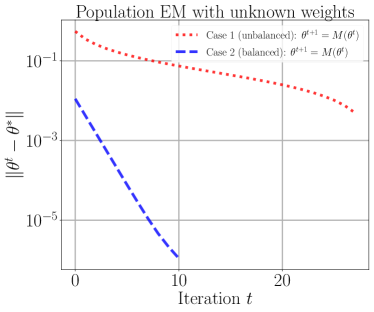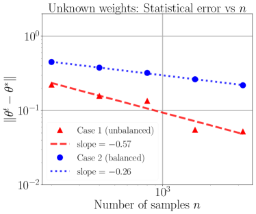(a)	(b)

Figure 10: Behavior of EM for the two-mixture over-specified fit (2) with unknown weights where the true model is $\mathcal{N}(0,I_{2})$. We consider two different initializations. Case 1 (unbalanced): When the initialization condition (81) is met (in particular we set $\uppi$ much smaller than $\frac{1}{2}$). In Case 2 (balanced), we initialize the weight parameter very close to $\frac{1}{2}$. Panel (a) characterizes the population EM updates and panel (b) depicts the statistical error with sample size $n$ for the two cases. We see that when the condition (81) is met, EM converges in few steps within error $n^{-\frac{1}{2}}$ error and on the other hand when the initial weight is near $\frac{1}{2}$ we observe a slow convergence of EM with a larger statistical error of order $n^{-\frac{1}{4}}$.

Corollary 1.

Consider the sample EM sequences $\pi^{t+1}=M_{1,n}(\uppi^{t})$ and $\theta^{t+1}=M_{2,n}(\theta^{t})$ with an initialization that satisfies the condition (81) for some $\overline{\pi}<1/2$. Then for any fixed $\delta\in(0,1)$ and $n\geq c\,d\log(1/\delta)\frac{\sigma^{2}}{\overline{\rho}^{4}}$, we have

$$\uppi^{t}\leq\overline{\uppi},\ \quad\ \left\|\theta^{t}\right\|_{2}\leq\left\|\theta^{0}\right\|_{2}\left[\left(1-{\overline{\rho}^{2}}/{2}\right)^{t}+\frac{c^{\prime}\sigma^{2}}{\overline{\rho}^{2}}\sqrt{\frac{d\log(1/\delta)}{n}}\;\right],$$ (82)

with probability at least $1-\delta$, where $c,c^{\prime}$ and $\overline{\rho}=1-2\overline{\pi}\in(0,1)$ are universal constants.

The proof is fairly straightforward given the proof of Theorem 1 and is thereby omitted. However, it remains to prove Lemma 6.

Proof of Lemma 6

The upper bound for $\left\|M_{2}(\theta,\uppi)\right\|_{2}$ follows directly from the proof of Theorem 1. Turning to the other bound in equation (80), we see that

$$\left|M_{1}(\theta,\uppi)-\uppi\right| =\uppi(1-\uppi)\left|{\mathbb{E}}_{X}\left[\dfrac{\exp\left(X^{\top}\theta\right)-\exp\left(-X^{\top}\theta\right)}{\uppi\exp\left(X^{\top}\theta\right)+(1-\uppi)\exp\left(-X^{\top}\theta\right)}\right]\right|$$

$$\leq 2\uppi(1-\uppi)\left\|\theta\right\|_{2}\max_{u\in[0,1]}|\!|\!|{\mathbb{E}}\left[\bar{\Gamma}_{\theta_{u}}(X)\right]|\!|\!|_{{\tiny{\mbox{op}}}},$$

where $\theta_{u}=u\theta$ for $u\in[0,1]$ and the matrix $\bar{\Gamma}_{\theta_{u}}(X)$ is defined as

$$\bar{\Gamma}_{\theta_{u}}(X):=\frac{X}{\sigma^{2}\left(\uppi\exp\left(-\frac{\theta_{u}^{\top}X}{\sigma^{2}}\right)+(1-\uppi)\exp\left(\frac{\theta_{u}^{\top}X}{\sigma^{2}}\right)\right)^{2}}.$$ (83)

Invoking the transformation as that from the proof of Theorem 1 and mimicking the arguments presented there, we can verify that

$$\left|{\mathbb{E}}_{X}\left[\bar{\Gamma}_{\theta_{u}}(X)\right]\right| =\left|{\mathbb{E}}_{V_{1}}\left[\dfrac{V_{1}}{\sigma\left(\uppi\exp\left(-\left\|\theta_{u}\right\|_{2}V_{1}/\sigma\right)+(1-\uppi)\exp\left(\left\|\theta_{u}\right\|_{2}V_{1}/\sigma\right)\right)^{2}}\right]\right|$$

$$\leq{\mathbb{E}}_{V_{1}}\left[\dfrac{\left|V_{1}\right|}{\sigma\left(\uppi\exp\left(-\left\|\theta_{u}\right\|_{2}V_{1}/\sigma\right)+(1-\uppi)\exp\left(\left\|\theta_{u}\right\|_{2}V_{1}/\sigma\right)\right)^{2}}\right]$$

$$\leq\dfrac{(1-\rho^{2})+\rho^{2}{\mathbb{E}}_{V_{1}}\left[\left|V_{1}\right|\mathbb{I}(V_{1}\geq 0)\right]}{(1-\rho^{2})}$$

$$=\frac{1-c\rho^{2}}{(1-\rho^{2})}$$

where $V_{1}\sim\mathcal{N}(0,1)$ and $c=1-{\mathbb{E}}_{V_{1}}\left[\left|V_{1}\right|\mathbb{I}(V_{1}\geq 0)\right]\in(1/2,1)$. Putting the above results together yields the claimed bound.

Appendix D Unbalanced vs balanced fits: Closer look at log-likelihood

In this appendix, we provide a further discussion on the difference between the unbalanced and balanced mixtures corresponding to the model  (2) considered throughout our work. Recall that the expected (population) log-likelihood for the model fit (2) is given by

$$\mathcal{L}^{\uppi}(\theta) ={\mathbb{E}}\left[\log\left(\uppi\phi\left(X;\theta,\sigma^{2}I_{d}\right)+(1-\uppi)\phi\left(X;-\theta,\sigma^{2}I_{d}\right)\right)\right],$$

where $\phi(\cdot;\theta,\sigma^{2}I_{d})$ denotes the probability density of the Gaussian distribution $\mathcal{N}(\theta,\sigma^{2}I_{d})$. Observe that

$$\arg\max_{\theta}\mathcal{L}^{\uppi}(\theta)=\arg\min_{\theta}\text{KL}(\mathcal{N}(0,\sigma^{2}I_{d})\|\uppi\mathcal{N}(\theta,\sigma^{2}I_{d})+(1-\uppi)\mathcal{N}(-\theta,\sigma^{2}I_{d})),$$

where $\text{KL}(P\|Q)$ denotes the Kullback-Leibler divergence between the distributions $P$ and $Q$. Since the true distribution belongs to the fitted class with $\theta^{*}=0$, finding maximizer of the population log-likelihood would yield the true parameter $\theta^{*}$. As alluded to in the main paper, in practical situations, when one has access to only $n$ i.i.d. samples $\{X_{i}\}_{i=1}^{n}$, the most popular choice to estimate $\theta^{*}$ is the maximum likelihood estimate (MLE) given by equation (4).

We now use the nature of log-likelihood to justify the difference between unbalanced and balanced fits. Note that the Fisher information matrix $\mathcal{I}^{\uppi}(\theta):=-\nabla^{2}_{\theta}\mathcal{L}^{\uppi}(\theta)$ for the fit (2) with mixture weights $(\uppi,1-\uppi)$ is given by

$$[\mathcal{I}^{\uppi}(\theta)]_{ii} =-4\uppi(1-\uppi){\mathbb{E}}\left[\frac{Y_{i}^{2}}{(\uppi\exp(\theta^{\top}Y)+(1-\uppi)\exp(-\theta^{\top}Y))^{2}}\right]+1$$

for $i\in[d]$ and

$$[\mathcal{I}^{\uppi}(\theta)]_{ij} =-4\uppi(1-\uppi){\mathbb{E}}\left[\frac{Y_{i}Y_{j}}{(\uppi\exp(\theta^{\top}Y)+(1-\uppi)\exp(-\theta^{\top}Y))^{2}}\right]$$

for $i,j\in[d]$ such that $i\neq j$. Here the expectations are taken under the true model $Y=(Y_{1},\ldots,Y_{d})\sim\mathcal{N}(0,I_{d})$. Clearly, at $\theta=\theta^{*}=0$, we have

$$\mathcal{I}^{\uppi}(\theta^{*})=\beta^{\uppi}I_{d},\quad\text{where}\quad\beta^{\uppi}=-4\uppi(1-\uppi)+1.$$ (84)

Note that $\beta^{\uppi}>0$ for any $\uppi\in(0,1)$ such that $\uppi\neq 1/2$. On the other hand, for $\uppi=1/2$, we have $\beta^{\uppi}=0$. Consequently, we find that for any unbalanced fit with $\uppi\neq 1/2$, the Fisher matrix is positive definite at $\theta^{*}$, and, for the balanced fit with $\uppi=1/2$, it is singular at $\theta^{*}$. Equivalently, the log-likelihood is strongly log-concave around $\theta^{*}$ for the unbalanced fit and weakly log-concave for the balanced fit.

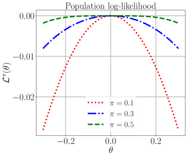(a)	(b)

Figure 11: Plots of the log-likelihood for the unbalanced and balanced fit for data generated from $\mathcal{N}(0,1)$. (a) Behavior of population log-likelihood $\mathcal{L}^{\uppi}$ (5) (computed using numerical integration) as a function of $\theta$ for different weights $\uppi\in\left\{0.1,0.3,0.5\right\}$. (b) Behavior of sample log-likelihood $\mathcal{L}_{n}^{\uppi}$ (4) with $n=1000$ samples for $\uppi\in\left\{0.1,0.3,0.5\right\}$. The plots in these panels portray a stark contrast in the shapes of the log-likelihood functions in the balanced and unbalanced case, it gets flatter around $\theta^{*}=0$ as $\uppi\to 0.5$. More concretely, in unbalanced case we see a quadratic type behavior (strongly concave); whereas in balanced case, the log-likelihood function is flatter and depicts a fourth degree polynomial type (weakly concave) behavior.

We numerically computed the population log-likelihood and plotted it in Figure 11(a), where we observe that when the mixture weights are unbalanced ($\uppi<1/2$), the population log-likelihood for the model has more curvature, and in fact is (numerically) well-approximated as $\mathcal{L}^{\uppi}(\theta)\approx-c^{\uppi}\theta^{2}$. On the other hand, for the balanced model with $\uppi=\frac{1}{2}$, the likelihood is quite flat near origin and is (numerically) well-approximated as $\mathcal{L}^{\uppi}(\theta)\approx-c\,\theta^{4}$. It is a folklore that the convergence rate of optimization methods has a phase transition: optimizing strongly concave functions is exponentially fast than weakly concave functions. As a result, we might expect why population EM may have fundamentally different rate of algorithmic convergence in the two model fits as observed in Figure 2 (in the main paper).

Moreover, the singularity of Fisher matrix is known to lead to a slow down the statistical rate of MLE. It is well established [29] that when the Fisher matrix is invertible in a neighborhood of the true parameter, MLE has the parametric rate of $n^{-\frac{1}{2}}$, i.e., the MLE estimate is at a distance of order $n^{-\frac{1}{2}}$ from the true parameter $\theta^{*}$. Moreover, as discussed in the introduction of the main paper, several works [4, 23] have also shown than the singularity of the Fisher matrix may lead to a slower than $n^{-\frac{1}{2}}$ rate for the MLE. Since EM algorithm is designed to estimate MLE (and converges only to local maxima), we may loosely conclude that, for the singular case (balanced fit), a slower than parametric rate for the EM estimate is also expected.

Appendix E Mixture of regression

In this appendix, we provide formal results for the slow convergence of EM for over-specified mixture of linear regression (as discussed in Section 5.2).

Given $n$ samples from the mixture of regressions model (26), we use EM to fit the following model:

$$Y|X\sim\frac{1}{2}\mathcal{N}(\theta^{\top}X,1)+\frac{1}{2}\mathcal{N}(-\theta^{\top}X,1),$$ (85)

where we assume the knowledge of covariate design $X\sim\mathcal{N}(0,I_{d})$. Given this joint model on $(X,Y)$ the population log-likelihood for the model is given by

$$\mathcal{L}(\theta)={\mathbb{E}}_{X,Y}\left[\log\left(\uppi\phi\left(Y;\theta^{\top}X,\sigma^{2}I_{d}\right)+(1-\uppi)\phi\left(Y;-\theta^{\top}X,\sigma^{2}I_{d}\right)\right)\right],$$

where $\phi(\cdot;\theta,\sigma^{2}I_{d})$ denotes the probability density of the Gaussian distribution $\mathcal{N}(\theta,\sigma^{2}I_{d})$. In Figure 12, we plot this log-likelihood as a function of $\theta$ for two different values of $\theta^{*}$ and observe the following. When the mixture has strong signal ($\theta^{*}=0.7$), the Hessian of log-likelihood is negative definite (strongly concave) but in the case of no signal $\theta^{*}=0$ the Hessian degenerates at $\theta^{*}$ and the log-likelihood becomes weakly concave.

Figure 12: Plots of the population log-likelihood for the mixture of regression model for $\theta^{*}\in\left\{0,0.7\right\}$. We see that while the log-likelihood is clearly locally strongly concave around $\theta^{*}$ when $\theta^{*}=0.7$, and it is rather flat (and weakly concave) for the case of no signal $\theta^{*}=0$. This flatness in log-likelihood results in a slower rate of algorithmic and statistical convergence of EM in this setting thereby providing further evidence of the usefulness of our analysis of EM.

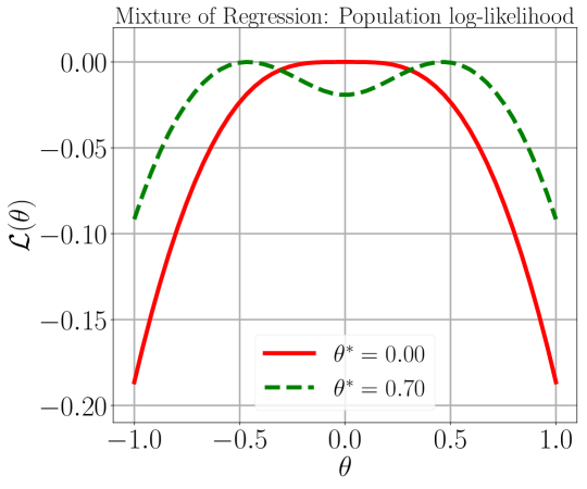The behavior observed in Figure 12 is reminiscent of the behavior of log-likelihood in the case of over-specified Gaussian mixtures considered in the main paper (see Appendix D and Figure 11). We now show that such a similarity also implies a similar behavior for EM, which converges slowly on both algorithmic and statistical fronts (just like the over-specified Gaussian mixture case) for the fit (85).

Given this model, the sample EM operator $\overline{M}_{n}:{}^{d}\mapsto{}^{d}$ takes the form

$$\overline{M}_{n}(\theta) :=\left(\sum_{i=1}^{n}X_{i}X_{i}^{\top}\right)^{-1}\left(\frac{1}{n}\sum_{i=1}^{n}(2w_{\theta}(X_{i},Y_{i})-1)X_{i}Y_{i}\right)$$ (86)

where we define

$$w_{\theta}(x,y):=\frac{\uppi\exp\left(-\frac{\left(y-\theta^{\top}x\right)^{2}}{2}\right)}{\uppi\exp\left(-\frac{\left(y-\theta^{\top}x\right)^{2}}{2}\right)+(1-\uppi)\exp\left(-\frac{\left(y+\theta^{\top}x\right)^{2}}{2}\right)}.$$ (87)

Consequently, the population EM operator $\overline{M}:{}^{d}\mapsto{}^{d}$ is given by

$$\overline{M}(\theta) :={\mathbb{E}}_{(Y,X)}\left[(2w_{\theta}(X,Y)-1)XY\right],$$ (88)

where the outer expectation is taken with respect to $X\sim\mathcal{N}(0,I_{d})$ and $Y|X\sim\mathcal{N}((\theta^{*})^{\top}X,1)$ ($=\mathcal{N}(0,I_{d})$ when $\theta^{*}=0$). Given these notation, we now characterize the slow convergence of the population EM operator:

Lemma 7.

Given the balanced model fit (85) to the true model (26) with $\theta^{*}=0$, the population EM operator $\overline{M}$ (88) satisfies the following bounds

$$\left\|\theta\right\|_{2}(1-3\left\|\theta\right\|_{2}^{2})\leq\left\|\overline{M}(\theta)\right\|_{2}\leq\left\|\theta\right\|_{2}(1-2\left\|\theta\right\|_{2}^{2})$$ (89)

for any $\theta\in\mathbb{R}^{d}$ such that $\left\|\theta\right\|_{2}\leq 1/2$.

Proof is deferred to the end of this appendix.

We note that the assumption $\left\|\theta\right\|_{2}\leq 1/2$ is a convenient technical assumption and is possibly loose in a similar manner as noted in Lemma 5 for the Gaussian mixture case. Applying the localization argument in the paper in conjunction with the sub-geometric convergence of the population EM (Lemma 7) yields the slow statistical convergence (of order $(d/n)^{\frac{1}{4}}$) of the sample EM:

Corollary 2.

Consider the over-specified model fit (85) to the true model (26) with $\theta^{*}=0$, and initialize the sample EM sequence $\theta^{t+1}=\overline{M}_{n}(\theta^{t})$ with a $\theta^{0}$ such that $\left\|\theta^{0}\right\|_{2}\leq\frac{1}{2}$. Then, for any $\varepsilon\in(0,1/4)$, $\delta\in(0,1)$, given a large sample size $n\geq c^{\prime}_{1}d\log(\log(1/\varepsilon)/\delta)$, the sample EM updates satisfy

$$\left\|\theta^{t}\right\|_{2}\leq\left[\left\|\theta^{0}\right\|_{2}\prod_{j=0}^{t-1}\left(1-2\left\|\theta^{j}\right\|_{2}^{2}\right)\right]+\sqrt{2}\left(\frac{(d+\log\frac{\log(4/\epsilon)}{\delta})}{n}\right)^{\frac{1}{4}-\epsilon},$$

for any iterate $t\geq c^{\prime}_{2}\left(\frac{n}{d}\right)^{\frac{1}{2}-2\varepsilon}\log(n/d)\log(1/\varepsilon)$, with probability at least $1-\delta$. Here, $c^{\prime}_{1}$ and $c^{\prime}_{2}$ denote universal constants.

Given Lemma 7, the proof of Corollary 2 follows the same annulus-based localization road-map as of the proof of Theorem 3; and is thereby omitted. We now prove Lemma 7.

Proof of Lemma 7

We provide a proof sketch for the lemma based on an application of Taylor expansion. In particular, we define a transformation $V:=RX$ where $R$ is an orthonormal matrix such that $R\theta=\left\|\theta\right\|_{2}e_{1}$ and $e_{1}$ denotes the first canonical basis vector in dimension $d$. After similar algebra as that of Theorem 2, we can verify that

$$\left\|\overline{M}(\theta)\right\|_{2}={\mathbb{E}}_{(Y,V_{1})}\left[\tanh(V_{1}Y\left\|\theta\right\|_{2})V_{1}Y\right],$$

where the outer expectation is taken with respect to $V_{1},Y\sim\mathcal{N}(0,1)$ and $V_{1}$ and $Y$ are independent. Using arguments similar to the bounds (55a) and (55b), we can derive that

$$x^{2}-\frac{x^{4}}{3}\leq\tanh(x)\leq x^{2}-\frac{x^{4}}{3}+\frac{2x^{6}}{15}$$

for all $x\in\mathbb{R}$. Given these bounds, we find that

$${\mathbb{E}}_{(Y,V_{1})}\left[\tanh(V_{1}Y\left\|\theta\right\|_{2})V_{1}Y\right]$$

$$\leq{\mathbb{E}}\left[(V_{1}Y)^{2}\right]\left\|\theta\right\|_{2}-\frac{{\mathbb{E}}\left[(V_{1}Y)^{4}\right]\left\|\theta\right\|_{2}^{3}}{3}+\frac{2{\mathbb{E}}\left[(V_{1}Y)^{6}\right]\left\|\theta\right\|_{2}^{5}}{15}$$

$$=\left\|\theta\right\|_{2}-3\left\|\theta\right\|_{2}^{3}+30\left\|\theta\right\|_{2}^{5}\leq\left\|\theta\right\|_{2}\left(1-2\left\|\theta\right\|_{2}^{2}\right),$$

and

$${\mathbb{E}}_{(Y,V_{1})}\left[\tanh(V_{1}Y\left\|\theta\right\|_{2})V_{1}Y\right] \geq{\mathbb{E}}\left[(V_{1}Y)^{2}\right]\left\|\theta\right\|_{2}-\frac{{\mathbb{E}}\left[(V_{1}Y)^{4}\right]\left\|\theta\right\|_{2}^{3}}{3}$$

$$=\left\|\theta\right\|_{2}-3\left\|\theta\right\|_{2}^{3}=\left\|\theta\right\|_{2}\left(1-3\left\|\theta\right\|_{2}^{2}\right)$$

for all $\theta\in\mathbb{R}^{d}$ such that $\left\|\theta\right\|_{2}\leq 1/2$. Putting the above results together yields the lemma.

References

- Balakrishnan, Wainwright and Yu [2017] {barticle}[author] \bauthor\bsnmBalakrishnan, \bfnmS.\binitsS., \bauthor\bsnmWainwright, \bfnmM. J.\binitsM. J. and \bauthor\bsnmYu, \bfnmB.\binitsB. (\byear2017). \btitleStatistical guarantees for the EM algorithm: From population to sample-based analysis. \bjournalThe Annals of Statistics \bvolume45 \bpages77-120. \endbibitem
- Bartlett, Bousquet and Mendelson [2005] {barticle}[author] \bauthor\bsnmBartlett, \bfnmP. L.\binitsP. L., \bauthor\bsnmBousquet, \bfnmO.\binitsO. and \bauthor\bsnmMendelson, \bfnmS.\binitsS. (\byear2005). \btitleLocal Rademacher complexities. \bjournalThe Annals of Statistics \bvolume33 \bpages1497–1537. \endbibitem
- Cai et al. [2019] {barticle}[author] \bauthor\bsnmCai, \bfnmT Tony\binitsT. T., \bauthor\bsnmMa, \bfnmJing\binitsJ., \bauthor\bsnmZhang, \bfnmLinjun\binitsL. \betalet al. (\byear2019). \btitleCHIME: Clustering of high-dimensional Gaussian mixtures with EM algorithm and its optimality. \bjournalThe Annals of Statistics \bvolume47 \bpages1234–1267. \endbibitem
- Chen [1995] {barticle}[author] \bauthor\bsnmChen, \bfnmJ.\binitsJ. (\byear1995). \btitleOptimal rate of convergence for finite mixture models. \bjournalThe Annals of Statistics \bvolume23 \bpages221-233. \endbibitem
- Chen [2018] {barticle}[author] \bauthor\bsnmChen, \bfnmY. C.\binitsY. C. (\byear2018). \btitleStatistical inference with local optima. \bjournalarXiv preprint arXiv:1807.04431. \endbibitem
- Chen and Li [2009] {barticle}[author] \bauthor\bsnmChen, \bfnmJ.\binitsJ. and \bauthor\bsnmLi, \bfnmP.\binitsP. (\byear2009). \btitleHypothesis test for normal mixture models: the EM approach. \bjournalThe Annals of Statistics \bvolume37 \bpages2523-2542. \endbibitem
- Daskalakis, Tzamos and Zampetakis [2017] {binproceedings}[author] \bauthor\bsnmDaskalakis, \bfnmC.\binitsC., \bauthor\bsnmTzamos, \bfnmC.\binitsC. and \bauthor\bsnmZampetakis, \bfnmM.\binitsM. (\byear2017). \btitleTen steps of EM suffice for mixtures of two Gaussians. In \bbooktitleProceedings of the 2017 Conference on Learning Theory. \endbibitem
- Dempster, Laird and Rubin [1997] {barticle}[author] \bauthor\bsnmDempster, \bfnmA. P.\binitsA. P., \bauthor\bsnmLaird, \bfnmN. M.\binitsN. M. and \bauthor\bsnmRubin, \bfnmD. B.\binitsD. B. (\byear1997). \btitleMaximum likelihood from incomplete data via the EM algorithm. \bjournalJournal of the Royal Statistical Society: Series B (Statistical Methodology) \bvolume39 \bpages1-38. \endbibitem
- Dwivedi et al. [2018] {binproceedings}[author] \bauthor\bsnmDwivedi, \bfnmR.\binitsR., \bauthor\bsnmHo, \bfnmN.\binitsN., \bauthor\bsnmKhamaru, \bfnmK.\binitsK., \bauthor\bsnmWainwright, \bfnmM. J.\binitsM. J. and \bauthor\bsnmJordan, \bfnmM. I.\binitsM. I. (\byear2018). \btitleTheoretical guarantees for EM under misspecified Gaussian mixture models. In \bbooktitleNeurIPS 31. \endbibitem
- Dwivedi et al. [2019] {barticle}[author] \bauthor\bsnmDwivedi, \bfnmRaaz\binitsR., \bauthor\bsnmHo, \bfnmNhat\binitsN., \bauthor\bsnmKhamaru, \bfnmKoulik\binitsK., \bauthor\bsnmWainwright, \bfnmMartin J\binitsM. J., \bauthor\bsnmJordan, \bfnmMichael I\binitsM. I. and \bauthor\bsnmYu, \bfnmBin\binitsB. (\byear2019). \btitleChallenges with EM in application to weakly identifiable mixture models. \bjournalarXiv preprint arXiv:1902.00194. \endbibitem
- Ghosal and van der Vaart [2001] {barticle}[author] \bauthor\bsnmGhosal, \bfnmS.\binitsS. and \bauthor\bparticlevan der \bsnmVaart, \bfnmA.\binitsA. (\byear2001). \btitleEntropies and rates of convergence for maximum likelihood and Bayes estimation for mixtures of normal densities. \bjournalThe Annals of Statistics \bvolume29 \bpages1233-1263. \endbibitem
- Hao et al. [2018] {barticle}[author] \bauthor\bsnmHao, \bfnmB.\binitsB., \bauthor\bsnmSun, \bfnmW.\binitsW., \bauthor\bsnmLiu, \bfnmY.\binitsY. and \bauthor\bsnmCheng, \bfnmG.\binitsG. (\byear2018). \btitleSimultaneous clustering and estimation of heterogeneous graphical models. \bjournalJournal of Machine Learning Research \bvolume18 \bpages1 - 58. \endbibitem
- Heinrich and Kahn [2018] {barticle}[author] \bauthor\bsnmHeinrich, \bfnmP.\binitsP. and \bauthor\bsnmKahn, \bfnmJ.\binitsJ. (\byear2018). \btitleStrong identifiability and optimal minimax rates for finite mixture estimation. \bjournalThe Annals of Statistics \bvolume46 \bpages2844-2870. \endbibitem
- Inglot [2010] {barticle}[author] \bauthor\bsnmInglot, \bfnmT.\binitsT. (\byear2010). \btitleInequalities for quantiles of the chi-square distribution. \bjournalProbability and Mathematical Statistics \bvolume30 \bpages339–351. \endbibitem
- Ishwaran, James and Sun [2001] {barticle}[author] \bauthor\bsnmIshwaran, \bfnmH.\binitsH., \bauthor\bsnmJames, \bfnmL. F.\binitsL. F. and \bauthor\bsnmSun, \bfnmJ.\binitsJ. (\byear2001). \btitleBayesian model selection in finite mixtures by marginal density decompositions. \bjournalJournal of the American Statistical Association \bvolume96 \bpages1316-1332. \endbibitem
- Janson [1997] {bbook}[author] \bauthor\bsnmJanson, \bfnmS.\binitsS. (\byear1997). \btitleGaussian Hilbert Spaces \bvolume129. \bpublisherCambridge University Press. \endbibitem
- Klusowski, Yang and Brinda [2019] {barticle}[author] \bauthor\bsnmKlusowski, \bfnmJason M\binitsJ. M., \bauthor\bsnmYang, \bfnmDana\binitsD. and \bauthor\bsnmBrinda, \bfnmWD\binitsW. (\byear2019). \btitleEstimating the coefficients of a mixture of two linear regressions by expectation maximization. \bjournalIEEE Transactions on Information Theory \bvolume65 \bpages3515–3524. \endbibitem
- Koltchinskii [2006] {barticle}[author] \bauthor\bsnmKoltchinskii, \bfnmV.\binitsV. (\byear2006). \btitleLocal Rademacher complexities and oracle inequalities in risk minimization. \bjournalThe Annals of Statistics \bvolume34 \bpages2593–2656. \endbibitem
- Kumar and Schmidt [2017] {barticle}[author] \bauthor\bsnmKumar, \bfnmR.\binitsR. and \bauthor\bsnmSchmidt, \bfnmM.\binitsM. (\byear2017). \btitleConvergence rate of expectation-maximization. \bjournal10th NIPS Workshop on Optimization for Machine Learning. \endbibitem
- Ledoux and Talagrand [1991] {bbook}[author] \bauthor\bsnmLedoux, \bfnmM.\binitsM. and \bauthor\bsnmTalagrand, \bfnmM.\binitsM. (\byear1991). \btitleProbability in Banach Spaces: Isoperimetry and Processes. \bpublisherSpringer-Verlag, New York, NY. \endbibitem
- Li, Chen and Marriott [2009] {barticle}[author] \bauthor\bsnmLi, \bfnmP.\binitsP., \bauthor\bsnmChen, \bfnmJ.\binitsJ. and \bauthor\bsnmMarriott, \bfnmP.\binitsP. (\byear2009). \btitleNon-finite Fisher information and homogeneity: an EM approach. \bjournalBiometrika \bvolume96 \bpages411-426. \endbibitem
- Ma, Xu and Jordan [2000] {barticle}[author] \bauthor\bsnmMa, \bfnmJ.\binitsJ., \bauthor\bsnmXu, \bfnmL.\binitsL. and \bauthor\bsnmJordan, \bfnmM. I.\binitsM. I. (\byear2000). \btitleAsymptotic convergence rate of the EM algorithm for Gaussian mixtures. \bjournalNeural Computation \bvolume12 \bpages2881-2907. \endbibitem
- Nguyen [2013] {barticle}[author] \bauthor\bsnmNguyen, \bfnmX.\binitsX. (\byear2013). \btitleConvergence of latent mixing measures in finite and infinite mixture models. \bjournalThe Annals of Statistics \bvolume4 \bpages370-400. \endbibitem
- Redner and Walker [1984] {barticle}[author] \bauthor\bsnmRedner, \bfnmRichard A\binitsR. A. and \bauthor\bsnmWalker, \bfnmHomer F\binitsH. F. (\byear1984). \btitleMixture densities, maximum likelihood and the EM algorithm. \bjournalSIAM review \bvolume26 \bpages195–239. \endbibitem
- Richardson and Green [1997] {barticle}[author] \bauthor\bsnmRichardson, \bfnmS.\binitsS. and \bauthor\bsnmGreen, \bfnmP. J.\binitsP. J. (\byear1997). \btitleOn Bayesian analysis of mixtures with an unknown number of components. \bjournalJournal of the Royal Statistical Society: Series B (Statistical Methodology) \bvolume59 \bpages731-792. \endbibitem
- Rousseau and Mengersen [2011] {barticle}[author] \bauthor\bsnmRousseau, \bfnmJ.\binitsJ. and \bauthor\bsnmMengersen, \bfnmK.\binitsK. (\byear2011). \btitleAsymptotic behaviour of the posterior distribution in overfitted mixture models. \bjournalJournal of the Royal Statistical Society: Series B (Statistical Methodology) \bvolume73 \bpages689-710. \endbibitem
- Stephens [2002] {barticle}[author] \bauthor\bsnmStephens, \bfnmM.\binitsM. (\byear2002). \btitleDealing with label switching in mixture models. \bjournalJournal of the Royal Statistical Society: Series B (Statistical Methodology) \bvolume62 \bpages795-809. \endbibitem
- van de Geer [2000] {bbook}[author] \bauthor\bparticlevan de \bsnmGeer, \bfnmS.\binitsS. (\byear2000). \btitleEmpirical Processes in M-estimation. \bpublisherCambridge University Press. \endbibitem
- van der Vaart [1998] {bbook}[author] \bauthor\bparticlevan der \bsnmVaart, \bfnmA. W.\binitsA. W. (\byear1998). \btitleAsymptotic Statistics. \bpublisherCambridge University Press. \endbibitem
- van der Vaart and Wellner [2000] {bbook}[author] \bauthor\bparticlevan der \bsnmVaart, \bfnmA. W.\binitsA. W. and \bauthor\bsnmWellner, \bfnmJ. A.\binitsJ. A. (\byear2000). \btitleWeak Convergence and Empirical Processes: With Applications to Statistics. \bpublisherSpringer-Verlag, New York, NY. \endbibitem
- Vershynin [2011] {barticle}[author] \bauthor\bsnmVershynin, \bfnmR.\binitsR. (\byear2011). \btitleIntroduction to the non-asymptotic analysis of random matrices. \bjournalarXiv:1011.3027v7. \endbibitem
- Wainwright [2019] {bbook}[author] \bauthor\bsnmWainwright, \bfnmM. J.\binitsM. J. (\byear2019). \btitleHigh-dimensional statistics: A non-asymptotic viewpoint. \bpublisherCambridge University Press, \baddressCambridge, UK. \endbibitem
- Wang et al. [2015] {binproceedings}[author] \bauthor\bsnmWang, \bfnmZ.\binitsZ., \bauthor\bsnmGu, \bfnmQ.\binitsQ., \bauthor\bsnmNing, \bfnmY.\binitsY. and \bauthor\bsnmLiu, \bfnmH.\binitsH. (\byear2015). \btitleHigh-dimensional expectation-maximization algorithm: Statistical optimization and asymptotic normality. In \bbooktitleAdvances in Neural Information Processing Systems 28. \endbibitem
- Wu [1983] {barticle}[author] \bauthor\bsnmWu, \bfnmC. F. Jeff\binitsC. F. J. (\byear1983). \btitleOn the convergence properties of the EM algorithm. \bjournalThe Annals of Statistics \bvolume11 \bpages95-103. \endbibitem
- Xu, Hsu and Maleki [2016] {binproceedings}[author] \bauthor\bsnmXu, \bfnmJ.\binitsJ., \bauthor\bsnmHsu, \bfnmD.\binitsD. and \bauthor\bsnmMaleki, \bfnmA.\binitsA. (\byear2016). \btitleGlobal analysis of expectation maximization for mixtures of two Gaussians. In \bbooktitleAdvances in Neural Information Processing Systems 29. \endbibitem
- Xu and Jordan [1996] {barticle}[author] \bauthor\bsnmXu, \bfnmL.\binitsL. and \bauthor\bsnmJordan, \bfnmM. I.\binitsM. I. (\byear1996). \btitleOn convergence properties of the EM Algorithm for Gaussian mixtures. \bjournalNeural Computation \bvolume8 \bpages129-151. \endbibitem
- Yan, Yin and Sarkar [2017] {binproceedings}[author] \bauthor\bsnmYan, \bfnmB.\binitsB., \bauthor\bsnmYin, \bfnmM.\binitsM. and \bauthor\bsnmSarkar, \bfnmP.\binitsP. (\byear2017). \btitleConvergence of gradient EM on multi-component mixture of Gaussians. In \bbooktitleAdvances in Neural Information Processing Systems 30. \endbibitem
- Yi and Caramanis [2015] {binproceedings}[author] \bauthor\bsnmYi, \bfnmX.\binitsX. and \bauthor\bsnmCaramanis, \bfnmC.\binitsC. (\byear2015). \btitleRegularized EM algorithms: a unified framework and statistical guarantees. In \bbooktitleAdvances in Neural Information Processing Systems 28. \endbibitem