Approximating mixed Hölder functions
using random samples

Abstract.

Suppose $f:[0,1]^{2}\rightarrow\mathbb{R}$ is a $(c,\alpha)$-mixed Hölder function that we sample at $l$ points $X_{1},\ldots,X_{l}$ chosen uniformly at random from the unit square. Let the location of these points and the function values $f(X_{1}),\ldots,f(X_{l})$ be given. If $l\geq c_{1}n\log^{2}n$, then we can compute an approximation $\tilde{f}$ such that

$$\|f-\tilde{f}\|_{L^{2}}=\mathcal{O}(n^{-\alpha}\log^{3/2}n),$$

with probability at least $1-n^{2-c_{1}}$, where the implicit constant only depends on the constants $c>0$ and $c_{1}>0$.

1. Introduction

1.1. Introduction

A function $f:[0,1]^{2}\rightarrow\mathbb{R}$ is $(c,\alpha)$-mixed Hölder if

$$|f(x^{\prime},y)-f(x,y)|\leq c|x^{\prime}-x|^{\alpha},\qquad|f(x,y^{\prime})-f(x,y)|\leq c|y^{\prime}-y|^{\alpha},$$

and

$$|f(x^{\prime},y^{\prime})-f(x,y^{\prime})-f(x^{\prime},y)+f(x,y)|\leq c(|x^{\prime}-x||y^{\prime}-y|)^{\alpha},$$

for all $x,x^{\prime},y,y^{\prime}\in[0,1]$. For example, if $f:[0,1]^{2}\rightarrow\mathbb{R}$ satisfies

$$\left|\frac{\partial f}{\partial x}\right|\leq c,\quad\left|\frac{\partial f}{\partial y}\right|\leq c,\quad\text{and}\quad\left|\frac{\partial f}{\partial x\partial y}\right|\leq c\quad\text{on $[0,1]^{2}$},$$

then by the mean value theorem $f$ is $(c,1)$-mixed Hölder. In 1963, Smolyak [5] discovered a surprising approximation result for mixed Hölder functions.

Lemma 1.1 (Smolyak).

Suppose that $f:[0,1]^{2}\rightarrow\mathbb{R}$ is $(c,\alpha)$-mixed Hölder. Then

$$f(x,y)=\sum_{k=0}^{m}f(x_{k},y_{m-k})-\sum_{k=1}^{m}f(x_{k-1},y_{m-k})+\mathcal{O}\left(m2^{-\alpha m}\right),$$

where $x_{k}$ is the center of the dyadic interval of length $2^{-k}$ that contains $x$, and $y_{j}$ is the center of the dyadic interval of length $2^{-j}$ that contains $y$.

Observe that the point $(x_{k},y_{j})$ is the center of a dyadic rectangle of width $2^{-k}$ and height $2^{-j}$; thus, Lemma 1.1 is a statement about approximating mixed Hölder functions by linear combinations of function values at the center of dyadic rectangles of area $2^{-m}$ and $2^{-m+1}$.

We remark that Smolyak [5] actually presented a general $d$-dimensional version of Lemma 1.1, and that the ideas of Smolyak were expanded upon by Strömberg [7], and have been developed into a computational tool called sparse grids, see [1]. The proof of Lemma 1.1 involves a telescoping series argument and is included below; throughout, we use the notation $f\lesssim g$ when $f\leq Cg$ for some constant $C>0$.

Proof of Lemma 1.1.

Fix $(x,y)\in[0,1]^{2}$. For notational brevity set $f_{k}^{j}:=f(x_{k},y_{j})$. First, we approximate $f(x,y)$ by the center $f_{m}^{m}$ of a $2^{-m}$ by $2^{-m}$ square. Clearly,

$$|f(x,y)-f_{m}^{m}|\lesssim 2^{-\alpha m}.$$

Expanding $f_{m}^{m}$ in successive telescoping series in $\{x_{k}\}_{k=1}^{m}$ and $\{y_{j}\}_{j=1}^{m}$ gives

$$f_{m}^{m}=\sum_{j=1}^{m}\sum_{k=1}^{m}\left(f_{k}^{j}-f_{k-1}^{j}-f_{k}^{j-1}+f_{k-1}^{j-1}\right)+\sum_{l=1}^{m}\left(f_{l}^{0}-f_{l-1}^{0}+f_{0}^{l}-f_{0}^{l-1}\right)+f_{0}^{0}.$$

Since $f$ is $(c,\alpha)$-mixed Hölder, it follows that the terms of the double sum satisfy

$$\left|f_{k}^{j}-f_{k-1}^{j}-f_{k}^{j-1}+f_{k-1}^{j-1}\right|\lesssim 2^{-\alpha(j+k)}.$$

Thus, we can bound the sum of terms in the double sum such that $j+k>m$ by

$$\sum_{j=1}^{m}\sum_{k=m-j+1}^{m}\left|f_{k}^{j}-f_{k-1}^{j}-f_{k}^{j-1}+f_{k-1}^{j-1}\right|\lesssim\sum_{j=1}^{m}\sum_{k=m-j+1}^{m}2^{-\alpha(j+k)}\lesssim m2^{-\alpha m}.$$

Removing these terms from the double sum and collapsing the telescoping series leaves only terms $f_{j}^{k}$ such that $j+k\in\{m,m-1\}$; in particular, we conclude that

$$\left|f_{m}^{m}-\left(\sum_{l=0}^{m}f_{l}^{m-l}-\sum_{l=1}^{m}f_{l-1}^{m-l}\right)\right|\lesssim m2^{-\alpha m},$$

which completes the proof. ∎

Remark 1.1.

The proof began by approximating $f(x,y)$ to error $\mathcal{O}(2^{-\alpha m})$ by the function value at the center of the dyadic square with side length $2^{-m}$ which contains $(x,y)$. However, it would require $2^{2m}$ function values to approximate $f$ at every point in the unit square using this method. In contrast, the telescoping argument in the proof of Lemma 1.1 achieves an approximation error of $\mathcal{O}(m2^{-\alpha m})$ while only using function values at the center of dyadic rectangles of area $2^{-m}$ and $2^{-m+1}$; the total number of such rectangles is $(m+1)2^{m}+m2^{m-1}$.

1.2. Main result

Informally speaking, Lemma 1.1 says that if we are given a specific set of $\sim n\ln n$ samples of a $(c,\alpha)$-mixed Hölder function $f:[0,1]^{2}\rightarrow\mathbb{R}$, then we are able to compute an approximation $\tilde{f}$ of $f$ such that

$$\|f-\tilde{f}\|_{L^{\infty}}=\mathcal{O}(n^{-\alpha}\log n),\quad\text{and}\quad\|f-\tilde{f}\|_{L^{2}}=\mathcal{O}(n^{-\alpha}\log n),$$

where the $L^{2}$-norm estimate follows directly from the $L^{\infty}$-norm estimate. Our main result relaxes the sampling requirement to $\sim n\log^{2}n$ random samples and achieves the same $L^{2}$-norm error estimate up to $\log$ factors.

Theorem 1.1.

Suppose $f:[0,1]^{2}\rightarrow\mathbb{R}$ is a $(c,\alpha)$-mixed Hölder function that we sample at $l$ points $X_{1},\ldots,X_{l}$ chosen uniformly at random from the unit square. Let the location of these points and the function values $f(X_{1}),\ldots,f(X_{l})$ be given. If $l\geq c_{1}n\log^{2}n$, then we can compute an approximation $\tilde{f}$ such that

$$\|f-\tilde{f}\|_{L^{2}}=\mathcal{O}(n^{-\alpha}\log^{3/2}n),$$

with probability at least $1-n^{2-c_{1}}$, where the implicit constant only depends on the constants $c>0$ and $c_{1}>0$.

When $\alpha>1/2$ the theorem implies that we can integrate mixed Hölder functions on the unit square with an error rate that is better than the Monte Carlo rate of $\mathcal{O}(n^{-1/2})$ with high probability.

Corollary 1.1.

Under the assumptions of Theorem 1.1, if $l\geq c_{1}n\log^{2}n$, then we can compute an approximation $I$ of the integral of $f$ on $[0,1]^{2}$ such that

$$\int_{[0,1]^{2}}f(x)dx=I+\mathcal{O}(n^{-\alpha}\log^{3/2}n),$$

with probability at least $1-n^{2-c_{1}}$.

The proof of this corollary follows immediately from the $L^{2}$-norm estimate from Theorem 1.1 and the Cauchy Schwarz inequality.

Remark 1.2.

The computational cost of computing $\tilde{f}$ is $\mathcal{O}(n\log^{3}n)$ operations of pre-computation, and then $\mathcal{O}(\log n)$ operations for each point evaluation. Furthermore, after pre-computation we can compute the integral of $\tilde{f}$ on the unit square in $\mathcal{O}(n)$ operations. The construction of $\tilde{f}$ is described in §3.

Remark 1.3.

An advantage of using random samples and Theorem 1.1 to approximate a mixed Hölder function over using samples at the center of dyadic rectangles and Lemma 1.1 is the ability to perform spin cycling. For simplicity of exposition, assume that $f:[0,1]^{2}\rightarrow\mathbb{R}$ is a mixed Hölder function on the torus. Let $X_{1},\ldots,X_{l}$ be chosen uniformly at random from $[0,1]^{2}$, and let the function values $f(X_{1}),\ldots,f(X_{l})$ be given. By Theorem 1.1 we can compute an approximation $\tilde{f}$ of the function $f$; however, as described in §3 the computation of $\tilde{f}$ is dependent on the dyadic decomposition of $[0,1]^{2}$, and this dependence will create artifacts. We call the following method of removing these artifacts spin cycling.

Let $\zeta\in[0,1]^{2}$ be given, and define $f_{\zeta}(x)=f(x-\zeta)$ where addition is performed on the torus. By considering the function values $f(X_{1}),\ldots,f(X_{l})$ as values of the function $f_{\zeta}$ at the uniformly random sample of points $X_{1}+\zeta,\ldots,X_{l}+\zeta$, we can use Theorem 1.1 to compute an approximation $\tilde{f}_{\zeta}$ of the function $f_{\zeta}$. It follows that $\tilde{f}_{\zeta}(x+\zeta)$ is an approximation of $f$ with the same accuracy guarantees as $\tilde{f}$. However, the shift $\zeta$ has changed the relation of the function values to the dyadic decomposition of $[0,1]^{2}$, and thus has changed the resulting artifacts. In general, we can consider a sequence of shifts $\zeta_{1},\ldots,\zeta_{q}\in[0,1]^{2}$ and define

$$\bar{f}(x)=\frac{1}{q}\sum_{k=1}^{q}\tilde{f}_{\zeta_{k}}(x+\zeta_{k})\quad\text{for}\quad x\in[0,1]^{2},$$

where $\tilde{f}_{\zeta_{j}}$ is the approximation of the function $f_{\zeta_{j}}$ computed via Theorem 1.1 using the shift operation described above. We say that $\bar{f}$ is an approximation via Theorem 1.1 with $q$ spin cycles. In §4.1 we provide empirical evidence that spin cycling removes artifacts. We note that when $l\geq c_{1}n\log^{2}n$ and $c_{1}>2+\log(q)/\log(n)$, it follows that the accuracy claims of Theorem 1.1 hold for all function $\tilde{f}_{\zeta_{j}}$ for $j=1,\ldots,q$ with high probability. The assumption that $f$ is mixed Hölder on the torus can be relaxed by handling the boundaries appropriately. We emphasize that spin cycling is not possible when using a fixed sample of points at the center of dyadic rectangles and Lemma 1.1 as any shift moves the points away from the center of dyadic rectangles, which is prohibitive for using Lemma 1.1.

2. Preliminaries

2.1. Notation

Let $\mathcal{D}$ denote the set of dyadic intervals in $[0,1]$; more precisely,

$$\mathcal{D}:=\left\{\left[(j-1)2^{-k},j2^{-k}\right)\subset\mathbb{R}:k\in\mathbb{Z}_{\geq 0}\wedge j\in\{1,\ldots,2^{k}\}\right\}.$$

We say that $R=I\times J$ is a dyadic rectangle in the unit square if $I,J\in\mathcal{D}$. The number of dyadic rectangles in the unit square of area $2^{-m}$ is

$$(m+1)2^{m}=\#\left\{R=I\times J:|R|=2^{-m}\wedge I,J\in\mathcal{D}\right\}.$$

In particular, for each $k=0,\ldots,m$ there are $2^{m}$ distinct dyadic rectangles of width $2^{-k}$ and height $2^{m-k}$, which are disjoint and cover the unit square. We illustrate the dyadic rectangles in the unit square of area at least $2^{-3}$ in Figure 1.

Figure 1. The dyadic rectangles of area at least $2^{-3}$ in the unit square.

Recall that Lemma 1.1 approximates the value $f(x)$ of a mixed Hölder function by a linear combination of the function values at the centers of dyadic rectangles of area $2^{-m}$ and $2^{-m+1}$ that contain the point $x$. Thus, with respect to the illustration in Figure 1, the approximation formula of Lemma 1.1 consists of adding the function values at the center of the dyadic rectangles in the lowest row which contain $x$, and subtracting the function values at the center of the dyadic rectangles in the second lowest row which contain $x$.

2.2. Randomized Kaczmarz

In addition to properties of dyadic rectangles, we will use a result of Strohmer and Vershynin [6] regarding the convergence of a randomized Kaczmarz algorithm. Specifically, Strohmer and Vershynin show that a specific randomized Kaczmarz algorithm converges exponentially fast at a rate that only depends on how well the matrix is conditioned. The following lemma is a special case of their result, which will be sufficient for our purposes.

Lemma 2.1 (Strohmer, Vershynin).

Let $A$ be an $N\times n$ matrix where $N\geq n$ whose rows are of equal magnitude, and let $Aw=b$ be a consistent linear system of equations. Suppose that $l$ indices $I_{1},\ldots,I_{l}$ are chosen uniformly at random from $\{1,\ldots,N\}$. Let an initial guess at the solution $v_{0}$ be given. For $k=1,\ldots,l$ define

$$v_{k}:=v_{k-1}+\frac{b_{I_{k}}-\langle a_{I_{k}},v_{k-1}\rangle}{\|a_{I_{k}}\|_{\ell^{2}}^{2}}a_{I_{k}},$$

where $a_{j}$ denotes the $j$-th row of $A$, and $b_{j}$ denotes the $j$-th entry of $b$. Then

$$\mathbb{E}\|v_{k}-w\|^{2}_{\ell^{2}}\leq(1-\kappa^{-2})^{k}\|v_{0}-w\|_{\ell^{2}}^{2},$$

for $k=1,\ldots,l$, where $\kappa^{2}:=\sum_{j=1}^{n}\sigma_{j}^{2}/\sigma_{n}^{2}$ and $\sigma_{1},\ldots,\sigma_{n}$ are the singular values of $A$.

The rate of convergence of the algorithm is determined by the constant $\kappa$, which only depends on the singular values of the matrix $A$. This constant $\kappa$ can be viewed as a type of condition number for the matrix $A$, and can be equivalently defined as the Frobenius norm of $A$ multiplied by the operator norm of the left inverse of $A$. We remark that the convergence of the randomized Kaczmarz algorithm for inconsistent linear systems $Aw\approx b+\varepsilon$ is analyzed by Needell [4]. In the proof of the main result we use Lemma 2.1 in combination with a modified version of the error analysis in [4].

2.3. Organization

The remainder of the paper consists of the proof of Theorem 1.1 in §3 followed by discussion in §4. The proof of Theorem 1.1 is organized as follows. In §3.1, we define an embedding of the points in the unit square into a larger finite dimensional vector space. In §3.2, we show that inner products of vectors with the defined embedding coordinates have a martingale interpretation. In §3.3, we show that mixed Hölder functions can be approximated by linear functionals in the embedding coordinates. In §3.4, we show that the randomized Kaczmarz algorithm can be used to solve a specifically constructed system. In §3.5, we use the developed tools to complete the proof of Theorem 1.1. Finally, in §3.6 we prove the computational cost claims of Remark 1.2.

3. Proof of Theorem 1.1

3.1. Embedding points

Recall, that there are $m2^{m-1}$ dyadic rectangles of area $2^{-m+1}$ in the unit square $[0,1]^{2}$. Let

$$T_{1},\ldots,T_{m2^{m-1}}$$

be an enumeration of these rectangles such that the rectangles

$$T_{k2^{m-1}+1},\ldots,T_{(k+1)2^{m-1}}$$

have width $2^{-k}$ and height $2^{k-m+1}$ for $k=0,\ldots,m-1$. Let $T^{+}_{j}$ and $T^{-}_{j}$ denote the left and right halves of $T_{j}$, respectively. Furthermore, let

$$R_{1},\ldots,R_{2^{m}}$$

be an enumeration of the dyadic rectangles of width $1$ and height $2^{-m}$.

Definition 3.1.

We define an embedding $\Psi:[0,1]^{2}\rightarrow\mathbb{R}^{(m+2)2^{m-1}}$ entry-wise by

$$\Psi_{j}(x)=\chi_{R_{j}}(x)\quad\text{for}\quad j=1,\ldots,2^{m},$$

and

$$\Psi_{2^{m}+j}(x)=\frac{1}{\sqrt{2}}\left(\chi_{T_{j}^{+}}(x)-\chi_{T_{j}^{-}}(x)\right),\quad\text{for}\quad j=1,\ldots,m2^{m-1},$$

where $\chi_{R}$ denotes the indicator function for the rectangle $R$.

Fix $x\in[0,1]^{2}$, and let $\beta_{0}$ be the index of the dyadic rectangle $R_{\beta_{0}}$ of width $1$ and height $2^{-m}$ that contains $x$. Then, for $k=1,\ldots,m$, let $\beta_{k}-2^{m}$ be the index of the dyadic rectangle $T_{\beta_{k}-2^{m}}$ of width $2^{-k+1}$ and height $2^{k-m}$ that contains $x$. Set $\xi_{0}:=\Psi_{\beta_{0}}(x)=1$, and

$$\xi_{k}:=\Psi_{\beta_{k}}(x)=\frac{1}{\sqrt{2}}\left(\chi_{T^{+}_{\beta_{k}-2^{m}}}(x)-\chi_{T^{-}_{\beta_{k}-2^{m}}}(x)\right),\quad\text{for}\quad k=1,\ldots,m,$$

such that $\xi_{k}$ is $+1/\sqrt{2}$ or $-1/\sqrt{2}$ depending on if $x$ is contained in the left or right half of $T_{\beta_{k}-2^{m}}$, respectively. Then, if $v\in\mathbb{R}^{(m+2)2^{m-1}}$ we have

$$\langle\Psi(x),v\rangle=\sum_{k=0}^{m}\xi_{k}v_{\beta_{k}},$$

where $\langle\cdot,\cdot\rangle$ denotes the $(m+2)2^{m-1}$-dimensional Euclidean inner product. In the following section we show that partial sums of this inner product can be interpreted as martingales.

3.2. Martingale interpretation

Suppose that $x\in[0,1]^{2}$ is chosen uniformly at random, and let the indices $\beta_{0},\ldots,\beta_{m}$ and the scalars $\xi_{0},\ldots,\xi_{m}$ be defined as above. Let $v\in\mathbb{R}^{(m+2)2^{m-1}}$ be a fixed unit vector. We define the partial sum $Y_{r}$ by

$$Y_{r}=\sum_{k=0}^{r}\xi_{k}v_{\beta_{k}},\quad\text{for}\quad r=0,\ldots,m.$$

We assert that $\{Y_{r}\}_{k=0}^{m}$ is a martingale with respect to $\{\beta_{0},\xi_{1},\ldots,\xi_{m}\}$, that is,

$$\mathbb{E}\left(Y_{k+1}\big{|}\beta_{0},\xi_{1},\ldots,\xi_{k}\right)=Y_{k},\quad\text{for}\quad k=0,\ldots,m-1.$$

Indeed, this martingale property can be seen by interpreting the partial sums from a geometric perspective. Recall that $\beta_{0}$ determines the dyadic rectangle $R_{\beta_{0}}$ of width $1$ and height $2^{-m}$ that contains $x$. Therefore, $\beta_{0}$ determines the dyadic rectangle $T_{\beta_{1}-2^{m}}$ of width $1$ and height $2^{-m+1}$ that contains $x$. However, $\beta_{0}$ provides no information about $\xi_{1}=\pm 1/\sqrt{2}$, which is positive or negative depending on if the point $x$ is in the left or right side of $T_{\beta_{1}-2^{m}}$, respectively. It follows that

$$\mathbb{E}\left(Y_{1}\big{|}\beta_{0}\right)=\frac{1}{2}\left(v_{\beta_{0}}+\frac{1}{\sqrt{2}}v_{\beta_{1}}\right)+\frac{1}{2}\left(v_{\beta_{0}}-\frac{1}{\sqrt{2}}v_{\beta_{1}}\right)=Y_{0}.$$

More generally, $\beta_{k}$ and $\xi_{k}$ determine $\beta_{k+1}$ since together $\beta_{k}$ and $\xi_{k}$ determine the dyadic rectangle $T_{\beta_{k}-2^{m}}^{\operatorname{sgn}\xi_{k}}$ of width $2^{-k}$ and height $2^{m-k}$, which contains $x$. This, in turn, determines the rectangle $T_{\beta_{k+1}-2^{m}}$ of width $2^{-k}$ and height $2^{k-m+1}$ which contains $x$, but provides no information about which side (left or right) of this rectangle the point $x$ is contained in, that is to say, no information about $\xi_{k+1}$. Hence

$$\mathbb{E}\left(Y_{k+1}\big{|}\beta_{0},\xi_{1},\ldots,\xi_{k}\right)=\frac{1}{2}\left(Y_{k}+\frac{1}{\sqrt{2}}v_{\beta_{k+1}}\right)+\frac{1}{2}\left(Y_{k}-\frac{1}{\sqrt{2}}v_{\beta_{k+1}}\right)=Y_{k}.$$

This martingale property of the partial sums has several useful consequences.

Lemma 3.1.

Suppose that $X$ is chosen uniformly at random from the unit square, and set $Y=\Psi(X)$. Let $v\in\mathbb{R}^{(m+2)2^{m-1}}$ be a fixed vector of unit length. Then,

$$\mathbb{E}|\langle Y,v\rangle|^{2}=2^{-m}.$$

Proof.

Let $\beta_{0},\ldots,\beta_{m}$ and $\xi_{0},\ldots,\xi_{m}$ be as defined above such that

$$\mathbb{E}|\langle Y,v\rangle|^{2}=\mathbb{E}\left|\sum_{k=0}^{m}\xi_{k}v_{\beta_{k}}\right|^{2}=\sum_{k_{1},k_{2}=0}^{m}\mathbb{E}\xi_{k_{1}}\xi_{k_{2}}v_{\beta_{k_{1}}}v_{\beta_{k_{2}}}.$$

If $k_{1}>k_{2}$, then $\xi_{k_{2}}$ and $\beta_{k_{2}}$ are determined by $\beta_{0},\xi_{1},\ldots,\xi_{{k_{1}}-1}$; we conclude that

$$\mathbb{E}\left(\xi_{k_{1}}\xi_{k_{2}}v_{\beta_{k_{1}}}v_{\beta_{k_{2}}}\right)=\mathbb{E}\left(\xi_{k_{2}}v_{\beta_{k_{2}}}\mathbb{E}\left(\xi_{k_{1}}v_{\beta_{k_{1}}}\big{|}\beta_{0},\xi_{1},\ldots,\xi_{k_{1}-1}\right)\right)=0,$$

where the finally equality follows from the fact that the expected value of $\xi_{k_{1}}v_{\beta_{k_{1}}}$ conditional on $\beta_{0},\xi_{1},\ldots,\xi_{k_{1}-1}$ is zero by the above described martingale property. An identical argument holds for the case when $k_{1}<k_{2}$ so it follows that

$$\sum_{k_{1},k_{2}=0}^{m}\mathbb{E}\xi_{k_{1}}\xi_{k_{2}}v_{\beta_{k_{1}}}v_{\beta_{k_{2}}}=\sum_{k=0}^{m}\mathbb{E}\xi_{k}^{2}v_{\beta_{k}}^{2}=\mathbb{E}v_{\beta_{0}}^{2}+\frac{1}{2}\sum_{k=1}^{m}\mathbb{E}v_{\beta_{k}}^{2}.$$

We can compute this expectation explicitly by noting that the probability that $x$ is contained a given dyadic rectangle is proportional to its area; specifically, we have

$$\mathbb{E}v_{\beta_{0}}^{2}+\frac{1}{2}\sum_{k=1}^{m}\mathbb{E}v_{\beta_{k}}^{2}=\frac{1}{2^{m}}\sum_{j=1}^{2^{m}}v_{j}^{2}+\frac{1}{2}\frac{1}{2^{m-1}}\sum_{k=1}^{m}\sum_{j=1}^{2^{m-1}}v_{(k+1)2^{m-1}+j}^{2}=2^{-m},$$

where the final equality follows from collecting terms and using the assumption that $v$ is a unit vector in $\mathbb{R}^{(m+2)2^{m-1}}$. ∎

Since embedding $\Psi:[0,1]^{2}\rightarrow\mathbb{R}^{(m+2)2^{m-1}}$ is defined using indicator functions of dyadic rectangles of area $2^{-m}$ in $[0,1]^{2}$, it follows that $\Psi$ is constant on $2^{-m}$ by $2^{-m}$ dyadic squares since all points in such a square are contained in the same collection of dyadic rectangles of area $2^{-m}$ in $[0,1]^{2}$. This observation leads the following corollary of Lemma 3.1.

Corollary 3.1.

Let $x_{1},\ldots,x_{2^{2m}}$ be a sequence of points such that each $2^{-m}$ by $2^{-m}$ dyadic square contains exactly one point. Let $A$ be the $2^{2m}\times(m+2)2^{m-1}$ matrix whose $j$-th row is $\Psi(x_{j})$. Then,

$$\sigma_{1}=\cdots=\sigma_{(m+2)2^{m-1}}=2^{m/2},$$

where $\sigma_{1},\ldots,\sigma_{(m+2)2^{m-1}}$ are the singular values of $A$.

Proof.

Let $v\in\mathbb{R}^{(m+2)2^{m-1}}$ be an arbitrary unit vector. We have

$$\|Av\|_{\ell^{2}}^{2}=\sum_{j=1}^{2^{2m}}|\langle\Psi(x_{j}),v\rangle|^{2}.$$

However, since all points in each $2^{-m}$ by $2^{-m}$ dyadic square have the same embedding, and since the measures of all such dyadic squares are equal, we have

$$\sum_{j=1}^{2^{2m}}|\langle\Psi(x_{j}),v\rangle|^{2}=2^{2m}\mathbb{E}|\langle Y,v\rangle|^{2},$$

where $Y:=\Psi(X)$ for a point $X$ chosen uniformly at random from the unit square. By Lemma 3.1 we conclude that

$$\|Av\|_{\ell^{2}}^{2}=2^{2m}\mathbb{E}|\langle Y,v\rangle|^{2}=2^{m},$$

and since $v$ was an arbitrary unit vector the proof is complete. ∎

3.3. Approximation by linear functionals

So far we have constructed an embedding $\Psi:[0,1]^{2}\rightarrow\mathbb{R}^{(m+2)2^{m-1}}$, and we have shown that inner products of the form $\langle\Psi(X),v\rangle$ are related to martingales. We have used this relation to show that the collection of all possible embedding vectors form a matrix whose singular values are all $2^{m/2}$. Next, we show that a mixed Hölder function can be approximated by a linear functional in the embedding coordinates.

Lemma 3.2.

Let $f:[0,1]^{2}\rightarrow\mathbb{R}$ be a $(c,\alpha)$-mixed Hölder function. Then, there exists a vector $w\in\mathbb{R}^{(m+2)2^{m-1}}$ such that

$$f(x)=\langle\Psi(x),w\rangle+\mathcal{O}(m2^{-\alpha m}),\quad\text{for all}\quad x\in[0,1]^{2},$$

where the vector $w$ depends on $f$, but is independent of $x$ and is explicitly defined below in Definition 3.2.

We construct the vector $w$ using a scheme similar to the construction of Haar wavelets. Let $\mathcal{D}_{k}^{j}$ be the collection of dyadic rectangles contained in the unit square of width $2^{-k}$ and area $2^{-j}$. For a given dyadic rectangle $R$, we define $s_{r}(R)$ by

$$s_{r}(R):=\sum_{R^{\prime}\in\mathcal{D}_{r}^{m}:|R\cap R^{\prime}|>0}f(c_{R^{\prime}})-\sum_{R^{\prime}\in\mathcal{D}_{r}^{m-1}:|R\cap R^{\prime}|>0}f(c_{R^{\prime}}),$$

where $c_{R^{\prime}}$ is the center of $R^{\prime}$. Observe that the first sum in the definition of $s_{r}(R)$ is over the dyadic rectangles of width $2^{-r}$ and area $2^{-m}$ that intersect $R$, while the second sum is over the dyadic rectangles of width $2^{-r}$ and area $2^{-m+1}$ that intersect $R$.

Definition 3.2.

We define the vector $w\in\mathbb{R}^{(m+2)2^{m-1}}$ entry-wise by

$$w_{j}=\sum_{r=0}^{m}2^{-r}s_{r}\left(R_{j}\right)\quad\text{for}\quad j=1,\ldots,2^{m},$$

and

$$w_{2^{m}+j}=\frac{2^{k_{j}}}{\sqrt{2}}\sum_{r=k_{j}}^{m}2^{-r}\left(s_{r}\left(T_{j}^{+}\right)-s_{r}\left(T_{j}^{-}\right)\right),\quad\text{for}\quad j=1,\ldots,m2^{m-1},$$

where $k_{j}:=\lfloor j2^{-k}\rfloor$ is such that $2^{-k_{j}}$ is the width of the rectangle $T_{j}$.

Proof of Lemma 3.2.

Let $x$ be a fixed point in the unit square $[0,1]^{2}$. Recall that we can express the inner product

$$\langle\Psi(x),w\rangle=\sum_{k=0}^{m}\xi_{k}w_{\beta_{k}},$$

where the scalars $\xi_{0},\ldots,\xi_{m}$ and the indicies $\beta_{0},\ldots,\beta_{m}$ are as defined above. First, let us rewrite Lemma 1.1 using this notation. We have

$$f(x)=f\left(c_{R_{\beta_{0}}}\right)+\sum_{k=1}^{m}f\left(c_{T_{\beta_{k}-2^{m}}^{\operatorname{sgn}\xi_{k}}}\right)-\sum_{k=1}^{m}f\left(c_{T_{\beta_{k}-2^{m}}}\right)+\mathcal{O}(m2^{-\alpha m}).$$

Indeed, by definition $R_{\beta_{0}}$ is the dyadic rectangle of width $1$ and height $2^{-m}$ that contains $x$, $T_{\beta_{k}-2^{m}}^{\operatorname{sgn}\xi_{k}}$ is the dyadic rectangle of width $2^{-k}$ and height $2^{m-k}$ that contains $x$, and $T_{\beta_{k}-2^{m}}$ is the dyadic rectangle of width $2^{-k+1}$ and height $2^{m-k}$ that contains $x$. Thus, to complete the proof it suffices to show that

$$\sum_{k=0}^{m}\xi_{k}w_{\beta_{k}}=f\left(c_{R_{\beta_{0}}}\right)+\sum_{k=1}^{m}f\left(c_{T_{\beta_{k}-2^{m}}^{\operatorname{sgn}\xi_{k}}}\right)-\sum_{k=1}^{m}f\left(c_{T_{\beta_{k}-2^{m}}}\right).$$

Let us start by considering the terms $\xi_{0}w_{\beta_{0}},\ldots,\xi_{m}w_{\beta_{m}}$ of the summation expression for the inner product $\langle\Psi(x),w\rangle$. By the defintion of $w$ we have

$$\xi_{0}w_{\beta_{0}}=s_{0}(R_{\beta_{0}})+\sum_{r=1}^{m}2^{-r+1}\frac{s_{r}(T_{\beta_{1}}^{+})+s_{r}(T_{\beta_{1}}^{-})}{2},$$

and

$$\xi_{k}w_{\beta_{k}}=\sum_{r=k}^{m}2^{-r+k}\operatorname{sgn}\xi_{k}\frac{s_{r}\left(T_{\beta_{k}-2^{m}}^{+}\right)-s_{r}\left(T_{\beta_{k}-2^{m}}^{-}\right)}{2}.$$

for $k=1,\ldots,m$. We assert that if we start summing at $r=k+1$ we have

$$\sum_{r=k+1}^{m}2^{-r+k}s_{r}\left(T_{\beta_{k}-2^{m}}^{\operatorname{sgn}\xi_{k}}\right)=\sum_{r=k+1}^{m}2^{-r+k+1}\frac{s_{r}\left(T_{\beta_{k}-2^{m}}^{+}\right)+s_{r}\left(T_{\beta_{k}-2^{m}}^{-}\right)}{2}.$$

Indeed, observe that $T_{\beta_{k}-2^{m}}^{\operatorname{sgn}\xi_{k}}$ is the dyadic rectangle of width $2^{-k}$ and height $2^{m-k}$ that contains $x$. We have that

$$T_{\beta_{k}-2^{m}}^{\operatorname{sgn}\xi_{k}}\subset T_{\beta_{k+1}-2^{m}}^{+}\cup T_{\beta_{k+1}-2^{m}}^{-}=T_{\beta_{k+1}-2^{m}},$$

since $T_{\beta_{k+1}-2^{m}}$ is the dyadic rectangle of width $2^{-k}$ and height $2^{k-m+1}$ that contains $x$. However, when $r\geq k+1$ we are summing of dyadic rectangles of height at least $2^{m-k+1}$, and any dyadic rectangle of height at least $2^{k-m+1}$ that intersects $T_{\beta_{k+1}-2^{m}}$ must also intersect $T_{\beta_{k}-2^{m}}^{\operatorname{sgn}\xi_{k}}$ so we conclude the above equality. By applying the identity iteratively as we add each term $\xi_{k}w_{\beta_{k}}$ we conclude that

$$\sum_{k=0}^{m}\xi_{k}w_{\beta_{k}}=s_{0}(R_{\beta_{0}})+\sum_{k=1}^{m}s_{r}\left(T_{\beta_{k}-2^{m}}^{\operatorname{sgn}\xi_{k}}\right).$$

Next, we observe that

$$s_{0}(R_{\beta_{0}})=f\left(c_{R_{\beta_{0}}}\right)-f\left(c_{T_{\beta_{1}-2^{m}}}\right),$$

and that for $k=1,\ldots,m-1$.

$$s_{k}\left(T_{\beta_{k}-2^{m}}^{\operatorname{sgn}\xi_{k}}\right)=f\left(c_{T_{\beta_{k}-2^{m}}^{\operatorname{sgn}\xi_{k}}}\right)-f\left(c_{T_{\beta_{k+1}-2^{m}}}\right).$$

However, observe that when $r=m$ we have

$$s_{m}(R):=\sum_{R^{\prime}\in\mathcal{D}_{m}^{m}:|R\cap R^{\prime}|>0}f(c_{R^{\prime}})-\sum_{R^{\prime}\in\mathcal{D}_{m}^{m-1}:|R\cap R^{\prime}|>0}f(c_{R^{\prime}}),$$

and there are no rectangles in the set $\mathcal{D}_{m}^{m-1}$, which is the set of rectangles of width $2^{-m}$ and area $2^{-m+1}$ that are contained in the unit square; indeed, such a rectangle would need to have height $2$, which is prohibitive. We conclude that

$$s_{m}\left(T_{\beta_{m}-2^{m}}^{\operatorname{sgn}\xi_{m}}\right)=f\left(c_{T_{\beta_{m}-2^{m}}^{\operatorname{sgn}\xi_{m}}}\right),$$

Recall that we have already shown that

$$\sum_{k=0}^{m}\xi_{k}w_{\beta_{k}}=s_{0}(R_{\beta_{0}})+\sum_{k=1}^{m}s_{k}\left(T_{\beta_{k}-2^{m}}^{\operatorname{sgn}\xi_{k}}\right);$$

substituting in the derived expressions for $s_{0}(R_{\beta_{0}})$ and $s_{k}(T_{\beta_{k}}^{\operatorname{sgn}\xi_{k}})$ gives

$$\sum_{k=0}^{m}\xi_{k}w_{\beta_{k}}=f\left(c_{R_{\beta_{0}}}\right)+\sum_{k=1}^{m}f\left(c_{T_{\beta_{k}-2^{m}}^{\operatorname{sgn}\xi_{k}}}\right)-\sum_{k=1}^{m}f\left(c_{T_{\beta_{k}-2^{m}}}\right),$$

which completes the proof. ∎

3.4. Random projections

We have established that in the embedding coordinates $\Psi(x)$ of a point $x\in[0,1]^{2}$ that Smolyak’s Lemma can be rephrased as a result about approximating mixed Hölder functions by linear functionals. Moreover, using the martingale interpretation of inner products of vectors with $\Psi(x)$ we were able to explicitly compute the singular values of the matrix of all possible embedding vectors. In the following we combine these ideas using the randomized Kaczmarz algorithm of Strohmer and Vershynin [6].

Suppose that $x_{1},\ldots,x_{2^{2m}}$ is a sequence of points that contains exactly one point in each $2^{-m}$ by $2^{-m}$ dyadic square in $[0,1]^{2}$. Let $A$ be the $2^{2m}\times(m+2)2^{m-1}$ dimensional matrix whose $j$-th row is $\Psi(x_{j})$. Since the embedding $\Psi(x)$ has $1$ entry of magnitude $1$ and $m$ entries of magnitude $1/\sqrt{2}$, see Definition 3.1, we have

$$\|\Psi(x)\|_{\ell^{2}}=\sqrt{1+m/2},$$

for all $x\in[0,1]^{2}$, and it follows that all of the rows of $A$ have equal magnitude. Suppose that $f:[0,1]^{2}\rightarrow\mathbb{R}$ is a $(c,\alpha)$-mixed Hölder function. By Lemma 3.2, there exists a vector $w$ such that

$$|f(x)-\langle\Psi(x),w\rangle|\lesssim m2^{-\alpha m}.$$

Define

$$\bar{f}(x):=\langle\Psi(x),w\rangle,$$

for all $x\in[0,1]^{2}$. If $b$ is the $2^{2m}$-dimensional vector whose $j$-th entry is $\bar{f}(x_{j})$, then we have a consistent linear system of equations

$$Aw=b.$$

By Corollary 3.1 the condition number $\kappa^{2}$ of $A$ satisfies

$$\kappa^{2}:=\sum_{j=1}^{(m+2)2^{m-1}}\sigma_{j}^{2}/\sigma_{(m+2)2^{m-1}}^{2}=(m+2)2^{m-1},$$

where $\sigma_{1},\ldots,\sigma_{(m+2)2^{m-1}}$ are the singular values of $A$. Observe that sampling points uniformly at random from $[0,1]^{2}$ and applying the embedding $\Psi$ is equivalent to choosing rows uniformly at random from $A$. Thus, the following result is a direct consequence of applying Lemma 2.1 to the consistent linear system of equations $Aw=b$ that we constructed above.

Lemma 3.3.

Suppose that $l$ points $X_{1},\ldots,X_{l}$ are sampled uniformly at random from $[0,1]^{2}$. Given an initial vector $v_{0}\in\mathbb{R}^{(m+2)2^{m-1}}$, define

$$v_{k}:=v_{k-1}+\frac{\bar{f}(X_{k})-\langle\Psi(X_{k}),v_{k-1}\rangle}{1+m/2}\Psi(X_{k}).$$

Then,

$$\mathbb{E}\|v_{k}-w\|^{2}_{\ell^{2}}\leq\left(1-\frac{1}{(m+2)2^{m-1}}\right)^{k}\|v_{0}-w\|^{2}_{\ell^{2}},$$

for $k=1,\ldots,l$.

Note that $v_{k}$ is defined using $\bar{f}(x)$ rather than $f(x)$ so that the definition of $v_{k}$ corresponds to running the randomized Kaczmarz algorithm on the consistent linear system $Aw=b$. When we complete the proof of Theorem 1.1 in the following section, we estimate the error caused by replacing $\bar{f}(x)$ by $f(x)=\bar{f}(x)+\mathcal{O}(m2^{-\alpha m})$. We remark that the expected error for the randomized Kaczmarz algorithm for inconsistent linear systems is analyzed by Needell [4]. Since we need an error estimate that holds with high probability we perform a modified version of the error analysis of Needell.

3.5. Proof of Theorem 1.1

In this section, we combine the developed tools to complete the proof of Theorem 1.1.

Proof of Theorem 1.1.

Suppose that $f:[0,1]^{2}\rightarrow\mathbb{R}$ is a $(c,\alpha)$-mixed Hölder function that is sampled at $l$ points $X_{1},\ldots,X_{l}$ chosen uniformly at random from $[0,1]^{2}$. For some initial vector $v_{0}^{*}\in\mathbb{R}^{(m+2)2^{m-1}}$, define

$$v_{k}^{*}:=v_{k-1}^{*}+\frac{f(X_{k})-\langle\Psi(X_{k}),v_{k-1}^{*}\rangle}{1+m/2}\Psi(X_{k}),$$

for $k=1,\ldots,l$. Recall that by Lemma 3.2 there exists a vector $w$ such that

$$|f(x)-\langle\Psi(x),w\rangle|\lesssim m2^{-\alpha m},$$

and recall that $\bar{f}(x):=\langle\Psi(x),w\rangle$. Suppose that $\varepsilon_{k}:=f(X_{k})-\bar{f}(X_{k})$. We can write

$$v_{k}^{*}=v_{k}+e_{k},$$

where $v_{k}$ is the vector defined in Lemma 3.3 by

$$v_{k}:=v_{k-1}+\frac{\bar{f}(X_{k})-\langle\Psi(X_{k}),v_{k-1}\rangle}{1+m/2}\Psi(X_{k}),$$

and $e_{k}$ is an error term defined by

$$e_{k}:=e_{k-1}+\frac{\varepsilon_{k}-\langle\Psi(X_{k}),e_{k-1}\rangle}{1+m/2}\Psi(X_{k}).$$

By orthogonality we have

$$\|e_{k}\|_{\ell^{2}}^{2}=\left\|e_{k-1}-\frac{\langle\Psi(X_{k}),e_{k-1}\rangle}{1+m/2}\Psi(X_{k})\right\|^{2}_{\ell^{2}}+\frac{\varepsilon_{k}^{2}}{(1+m/2)^{2}}\|\Psi(X_{k})\|^{2}_{\ell^{2}}.$$

It follows that

$$\|e_{k}\|_{\ell^{2}}^{2}\leq\|e_{k-1}\|_{\ell^{2}}^{2}+\frac{\varepsilon_{k}^{2}}{1+m/2}\lesssim km2^{-2\alpha m}.$$

By the triangle inequality we have

$$\|v^{*}_{k}-w\|_{\ell^{2}}\lesssim\|v_{k}-w\|_{\ell^{2}}+\sqrt{km}2^{-\alpha m}.$$

Next, we estimate $\|v_{k}-w\|_{\ell^{2}}$. From Lemma 3.3 we have

$$\mathbb{E}\|v_{k}-w\|^{2}_{\ell^{2}}\leq\left(1-\frac{1}{(m+2)2^{m-1}}\right)^{k}\|v_{0}-w\|^{2}_{\ell^{2}}.$$

Thus, if $l\geq c_{1}\log(2^{m})(m+2)2^{m-1}$, then we have

$$\mathbb{E}\|v_{l}-w\|^{2}_{\ell^{2}}\leq 2^{-c_{1}m}\|v_{0}-w\|_{\ell^{2}}^{2}.$$

By the possibility of considering the function $f-f(X_{1})$ instead of $f$, we may assume that $|f|\leq 2c$ on $[0,1]^{2}$. It follows that $\|w\|_{\ell^{\infty}}\leq 3c$ when $m$ is large enough. Therefore, if we initialize $v_{0}$ as the zero vector we have

$$\|v_{0}-w\|_{\ell^{2}}^{2}\leq 9c^{2}(m+2)2^{m-1}.$$

From this estimate and our above analysis it follows that

$$\mathbb{E}\|v_{l}-w\|^{2}_{\ell^{2}}\leq\frac{9c^{2}}{2}(m+2)2^{(1-c_{1})m},$$

when $l\geq c_{1}\log(2^{m})(m+2)2^{m-1}$. Observe that

$$l=c_{1}\log(2^{m})(m+2)2^{m-1}\leq c_{1}\log^{2}(2^{m})2^{m},$$

when $m$ is sufficiently large. Thus, if $l\geq c_{1}\log^{2}(2^{m})2^{m}$, then by Markov’s inequality

$$\mathbb{P}(\|v_{l}-w\|_{\ell^{2}}^{2}\geq m^{3}2^{(1-2\alpha)m})\leq\frac{\mathbb{E}\|v_{l}-w\|_{\ell^{2}}^{2}}{m^{3}2^{(1-2\alpha)m}}\leq 2^{(2-c_{1})m},$$

when $m$ is large enough in terms of $c$. Recall that we previously showed that

$$\|v_{l}^{*}-w\|_{\ell^{2}}\lesssim\|v_{l}-w\|_{\ell^{2}}+\sqrt{ml}2^{-\alpha m}.$$

If $l=\lceil c_{1}\log(2^{m})^{2}2^{m}\rceil$, then by our estimate on $\|v_{l}-w\|_{\ell^{2}}$ it follows that

$$\|v_{l}^{*}-w\|_{\ell^{2}}\lesssim m^{3/2}2^{(1/2-\alpha)m},$$

with probability at least $1-2^{(2-c_{1})m}$. By Corollary 3.1, the operator norm of $A$ is $2^{m/2}$, so it follows that

$$\|Av_{l}^{*}-Aw\|_{\ell^{2}}\lesssim m^{3/2}2^{(1-\alpha)m},$$

with probability at least $1-2^{(2-c_{1})m}$. Thus, if we define the function $\tilde{f}:[0,1]^{2}\rightarrow\mathbb{R}$ by

$$\tilde{f}(x):=\langle\Psi(x),v_{l}^{*}\rangle,$$

then we have the estimate

$$\sqrt{\int_{[0,1]^{2}}|\tilde{f}(x)-\bar{f}(x)|^{2}dx}=\|\tilde{f}-\bar{f}\|_{L^{2}}\lesssim 2^{-\alpha m}m^{3/2},$$

with probability at least $1-2^{(2-c_{1})m}$. Since $\|\bar{f}-f\|_{L^{2}}\lesssim 2^{-\alpha m}m$ it follows that $\|\tilde{f}-f\|_{L^{2}}\lesssim 2^{-\alpha m}m^{3/2}$. Setting $n:=2^{m}$ completes the proof. ∎

3.6. Proof of Remark 1.2

It remains to verify the computational cost claims of Remark 1.2.

Proof of Remark 1.2.

Let $n=2^{m}$. The computation of $v_{l}^{*}$ described in Lemma 3.3 consists of $\mathcal{O}(n\log^{2}n)$ iterations of $\mathcal{O}(\log n)$ operations for a total of $\mathcal{O}(n\log^{3}n)$ operations of pre-computation. Then, since $\Psi(x)$ is supported on $\mathcal{O}(\log n)$ entries, the inner product $\langle\Psi(x),v_{l}^{*}\rangle$ requires $\mathcal{O}(\log n)$ operations. Finally, approximating the integral of $f$ amounts to approximating the function $f$ at each point, taking the sum, and dividing by $n^{2}$:

$$\left|\int_{[0,1]^{2}}f(x)-\frac{1}{n^{2}}\left\langle\sum_{j=1}^{n^{2}}\Psi(x_{j}),w\right\rangle\right|\lesssim n^{-\alpha}\log^{3/2}n.$$

However, this naive approach would require $\mathcal{O}(n^{2})$ operations. Instead, we make the observation that

$$\sum_{j=1}^{n^{2}}\Psi(x_{j})=g,$$

where $g$ is the vector whose first $n$ entries are equal to $1$ and which is zero elsewhere. Indeed, after the first $n$ entries, each entry is $+1/\sqrt{2}$ and $-1/\sqrt{2}$ for an equal number of embedding vectors. It follows that

$$\left|\int_{[0,1]^{2}}f(x)-\frac{1}{n}\left\langle g,w\right\rangle\right|\lesssim n^{-\alpha}\log^{3/2}n;$$

the computation of the inner product $\langle g,w\rangle$ only requires $\mathcal{O}(n)$ operations so the proof is complete. ∎

4. Discussion

4.1. Illustration

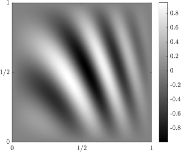
Suppose that $f:[0,1]^{2}\rightarrow\mathbb{R}$ is the function defined by

$$f(x,y)=\sin(20x^{2}+10y)\sin(\pi x)\sin(\pi y),\quad\text{for}\quad(x,y)\in[0,1]^{2}.$$

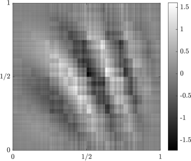
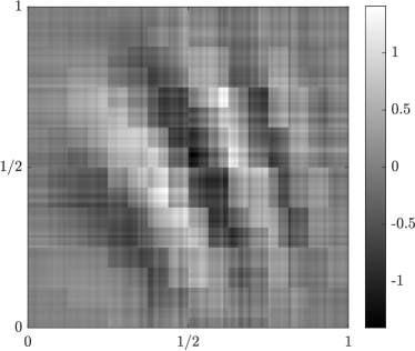
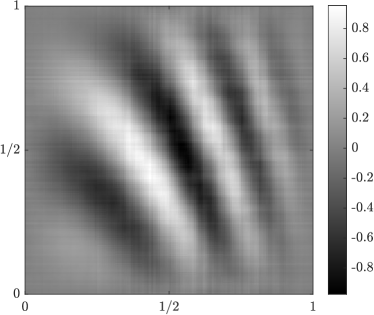
The function $f$ is $(c,1)$-mixed Hölder for some $c>0$ since the partial derivatives $\partial f/\partial x$, $\partial f/\partial y$, and $\partial^{2}f/(\partial x\partial y)$ are bounded in $[0,1]^{2}$. As a baseline, in Figure 2 we plot the function $f$, and the approximation of $f$ via the method of Smolyak (Lemma 1.1) with $m=7$ such that $n:=2^{m}=128$.

Figure 2. Function $f$ (left) and approximation via Lemma 1.1 (right).

Next, we set $c_{1}=8$ and sample $l=c_{1}n\log^{2}n$ points uniformly at random from $[0,1]^{2}$. In Figure 3, we plot the approximation of $f$ via Theorem 1.1, and the approximation of $f$ via Theorem 1.1 with $n=128$ spin cycles. In particular, the spin cycles are performed by considering $f$ as a function on the torus, generating a sequence of random shifts $\zeta_{1},\ldots,\zeta_{n}\in[0,1]^{2}$, and using the method of Remark 1.3.

Figure 3. Approximation via Theorem 1.1 (left) and approximation via Theorem 1.1 with $128$ spin cycles as in Remark 1.3 (right).

The plots in Figure 3 provide empirical evidence that spin cycling as described in Remark 1.3 reduces artifacts. Developing quantitative estimates for improvements in approximation accuracy resulting from spin cycling is an interesting theoretical problem for future study.

4.2. Discussion

There are several possible extensions and applications of Theorem 1.1. Informally speaking, we have shown that in $2$-dimensions the sampling requirements for the method of Smolyak [5] can be relaxed from a specific set of points at the center of dyadic rectangles to a similar number of random samples. As previously noted, Smolyak [5] presented a general $d$-dimensional version of Lemma 1.1 so an immediate question for future study is the extension of Theorem 1.1 to the $d$-dimensional cube. This would require defining a more sophisticated embedding $\Psi$ that retains an analog of the martingale property established in §3.2. It may also be interesting to consider generalizations of Theorem 1.1 to abstract dyadic trees as discussed by M. Gavish and R. R. Coifman in [2].

There are also interesting theoretical questions in $2$-dimensions related to random matrix theory. Given a collection of $l$ points $X_{1},\ldots,X_{l}$ chosen uniformly at random from $[0,1]^{2}$, we can consider the $l\times(m+2)2^{m-1}$ dimensional matrix $B$ whose $j$-th row is $\Psi(X_{j})$, where $\Psi$ is the embedding defined in Definition 3.1. The rows of $B$ are independent, and the inner product of a vector with a row of $B$ is a martingale sum, see §3.2. It would be interesting to develop quantitative high probability estimates on the singular values of $B$.

Finally, we note that the method of Smolyak [5] has been developed into a computational method called sparse grids, see [1]. The relaxation to random sampling and the ability to perform spin cycles may prove useful for certain applications. In particular, it may be interesting to consider applications of Theorem 1.1 in the Fourier domain, where the mixed Hölder condition is very natural. Recently, M. Griebel and J. Hamaekers [3] have developed a fast discrete Fourier transform on sparse grids, which could potentially be used in combination with Theorem 1.1.

Acknowledgements

The author would like to thank Raphy Coifman for many fruitful discussions.

References

- [1] H. Bungartz and M. Griebel. Sparse grids. Acta Numerica, 13:147–269, 2004.
- [2] M. Gavish and R. R. Coifman. Sampling, denoising and compression of matrices by coherent matrix organization. Applied and Computational Harmonic Analysis, 33(3):354–369, 2012.
- [3] M. Griebel and J. Hamaekers. Fast Discrete Fourier Transform on Generalized Sparse Grids. J. Garcke and D. Pflüger, editors. Sparse Grids and Applications - Munich 2012. Lecture Notes in Computational Science and Engineering, Vol. 97. Springer, Cham, 2014.
- [4] D. Needell. Randomized Kaczmarz solver for noisy linear systems. BIT, 50(2):395–403, 2010.
- [5] S. A. Smolyak. Quadrature and interpolation formulas for tensor products of certain classes of functions. Dokl. Akad. Nauk SSSR, 148(5):1042–1045, 1963.
- [6] T. Strohmer and R. Vershynin. A Randomized Kaczmarz Algorithm with Exponential Convergence. J. Fourier Anal. Appl., 15: 262–278, 2009.
- [7] J. O. Strömberg. Computation with Wavelets in Higher Dimensions. Doc. Math. J. DMV, 3:523–532, 1998.