Deep sequential models for sampling-based planning

Abstract

We demonstrate how a sequence model and a sampling-based planner can influence each other to produce efficient plans and how such a model can automatically learn to take advantage of observations of the environment. Sampling-based planners such as RRT generally know nothing of their environments even if they have traversed similar spaces many times. A sequence model, such as an HMM or LSTM, guides the search for good paths. The resulting model, called DeRRT^∗, observes the state of the planner and the local environment to bias the next move and next planner state. The neural-network-based models avoid manual feature engineering by co-training a convolutional network which processes map features and observations from sensors. We incorporate this sequence model in a manner that combines its likelihood with the existing bias for searching large unexplored Voronoi regions. This leads to more efficient trajectories with fewer rejected samples even in difficult domains such as when escaping bug traps. This model can also be used for dimensionality reduction in multi-agent environments with dynamic obstacles. Instead of planning in a high-dimensional space that includes the configurations of the other agents, we plan in a low-dimensional subspace relying on the sequence model to bias samples using the observed behavior of the other agents. The techniques presented here are general, include both graphical models and deep learning approaches, and can be adapted to a range of planners.

I INTRODUCTION

When you navigate an environment containing new agents, obstacles, and goals, you can rely on previous experiences to guide your actions. Having seen similar agents before allows you to predict the motions of the ones you encounter in the future. Having seen obstacles, whether static or dynamic, allows you to efficiently navigate around them. Having seen certain goal types allows you to determine what preconditions must be satisfied before meeting those goals. In each case, your expectations about the future of the plan are conditioned on your previous experiences, current plan, and local observations to help you navigate. This is the process we are modeling here.

Figure 1: A DeRRT^∗-based planner starts at the red square and tries to reach the green square while escaping from a bug trap. The search tree, shown as blue circles, is mirrored by a sequence model, an HMM or LSTM. When expanding the tree, a free-space sample is drawn, steered toward, and the resulting node, shown as a red circle, is used to find the closest node in the tree; as in RRT. The sequence model, with state corresponding to that closest node, observes this free-space sample, the path leading to this node, along with local visual or map features, shown in gray, and predicts a modified direction, shown in green, which is then connected to the search tree. A new state for the sequence model is also predicted and connected. This process incorporates the bias to explore free space of RRT-based planners with a co-evolving sequence model and observations of the environment.

Existing sampling-based planners have difficulty taking advantage of such information. Most planners, like RRT^∗ [1], sample uniformly and take no heed of the environment. RRT^∗, Rapidly-exploring Random Tree, is part of a family of algorithms [2, 3, 4, 5] that explore a configuration space by sampling moves while avoiding invalid states. Dynamic environments, in particular, pose many challenges. They combine uncertain sensing of the position of obstacles and agents with uncertainty about the future path of those obstacles and the actions being performed by other agents. To improve planning in these domains, we adopt a set of techniques from computer vision. We bias the growth of the RRT^∗ search tree [6, 7] given prior experience and a sensed environment. Hidden Markov Models (HMMs) [8], and stacked LSTMs [9] are powerful activity recognizers [10, 11, 12] but so far they have seen little use in improving robotic planning. We demonstrate how to adapt such sequence models to robotic planning using a general approach that can employ either graphical models or neural networks.

A sequence model co-evolves alongside a sampling-based planner as shown in Fig. 1. At each planning step, both the planner and the sequence model are stepped forward while the next sample from the planner is conditioned on the sequence model. That sequence model can observe local features of the environment as well as the current plan to provide good samples. Moreover, we can avoid feature engineering and learn the relevant features of the environment by co-training a convolutional network (CNN) with the LSTMs. We refer to this algorithm as DeRRT^∗, for deep RRT^∗, although the techniques presented here can be adapted to other sampling-based planners.

Several prior approaches have considered guiding planners with local observations of static and dynamic obstacles. Fulgenzi et al. [13] demonstrate how a Gaussian process can be combined with RRT to update plans conditioned on the observations of the motions of dynamic agents. This model estimates the positions of static and dynamic agents and assumes that the velocity and direction of motion are constant. Like the approach presented there, we plan incrementally and sample from the stochastic model at every timestep. Unlike this earlier work, we model the uncertainty in observing the position of obstacles by relying on the ability of the HMMs and LSTMs [14, 15] to capture this notion. Additionally, we also allow for obstacles and agents that change velocity or direction while including observations of features of those obstacles and agents. Features are learned entirely automatically in the case of LSTMs. Capturing the dynamics and appearance features of other entities can be helpful in predicting future behavior and enhancing planner performance. Aoude et al. [16] extend the work above to include a simulator which further constrains the possible trajectories of other agents. Such simulation is a natural extension to the models presented here using a range of probabilistic programming approaches [17] developed for computer vision [18] and robotics [19].

The closest work to our approach is that of Bowen and Alterovitz [20, 21]. Their approach learns an HMM model for the trajectory of plans which achieves a task and performs exhaustive inference in the cross-product space of that HMM and the configuration space of the planner. That work considers only domains where bidirectional planning is possible; we do not rely on such information here. Additionally, it only considers sequence models which observe the state of the configuration space and one additional feature, the distance between landmarks and the end effector. This prevents modeling the time-varying motion of other agents, although by detecting the arrival of new landmarks using a manually-set threshold, their approach can replan when the environment changes. This process does not account for perceptual uncertainty as to the position or even presence of objects. The inference algorithm considered in that work relies on a discrete HMM state. The approach presented here can employ either continuous HMMs or arbitrary deep learning sequence models such as stacked LSTMs or GRUs.

Similarly to the work above, Kim et al. [22] use a generative adversarial network, GAN [23], to learn an action sampler. At each timepoint, they sample a new action conditioned on the learned model. Unlike our approach, the GAN does not model the dynamics of other objects or capture uncertainty when sensing. Janson et al. [24] show a Monte-Carlo planning approach that, like the model described here, incorporates uncertainty in the observation of obstacles. It does not, however, consider the dynamics of obstacles or learn to extract relevant local features automatically. Arslan et al. [25] modify the steering function of a sampling-based planner, in their case PRM, to include sensory information. Unlike our approach, their work does not include a sequence model to model the dynamics of obstacles or other agents, or automatically learn to extract features from the environment.

Encoding the dynamics of other agents provides a major advantage: efficiently reasoning in multi-agent scenarios. Nominally the presence of other agents makes the reasoning problem exponentially harder. One must reason both about one’s configuration space and about the configuration space of the other agents. In the case of a single robotic arm manipulating an object, Schmitt et al. [26] show how, without needing any training, one can reduce the configuration space. Our method would be useful in this domain as it is more general at the expense of requiring training data. Work by Čáp et al. [27] and Chen et al. [28] demonstrates how planners, including sampling-based planners, can be adapted to multi-agent environments and cooperative planning without this exponential slowdown. Rather than cooperatively learning to plan, we demonstrate an agent avoidance task which relies on the sequence model to learn to avoid the other agents. Kiesel et al. [29] consider a related problem, learning to perform kinodynamic planning. Here we do not consider learning the dynamics of the robot being driven, instead only focusing on other agents and objects, but this would be an interesting direction for future work.

This work makes a number of contributions. We show how to combine sequence models with sampling-based planners in a manner that incorporates either graphical models or neural networks. Learned features of the trajectory, the local map, and the obstacles are combined together to improve the generated plans in novel environments. By borrowing its structure from computer vision algorithms for object tracking and activity recognition, the model incorporates perceptual uncertainty. The resulting model captures the dynamics of other agents to plan in multi-agent scenarios. Additionally, the model we present is flexible and can easily be adapted to new sampling-based planners. We demonstrate DeRRT^∗ with a classical narrow passage, a bug trap scenario, that co-trains a CNN to encode environmental cues, and a multi-agent scenario where we take advantage of the learned patterns of motion of the other agents. We expect that by employing general-purpose sequence models, which have seen great success in natural language processing and computer vision, to planning, this approach not only improves performance but opens the door to further cross-pollination between these areas.

II PLANNING WITH SEQUENCE MODELS

The algorithm presented here, DeRRT^∗, combines a sequence model with a sampling-based planner, RRT^∗. RRT-based algorithms create a tree which explores a configuration space. The tree is used to efficiently connect an initial state to a goal state in that configuration space. Given an initial state, RRT^∗ samples locations uniformly and then attempts to connect them to that original node. The tree reaches outward to cover the configuration space with a bias for large unexplored Voronoi cells, eventually finding paths to the goal state. In this way, RRT interleaves two steps: picking a point and steering toward it while avoiding obstacles and infeasible areas. See algorithm 1 for a prototypical RRT. RRT^∗ is an asymptotically optimal version of RRT [1]. There are a number of common extensions to RRT, for example, bidirectional RRT which considers the goal in addition to the initial state. The work presented here can easily be adapted to such enhanced RRTs.

Algorithm 1 A prototypical RRT algorithm.

1:$V\leftarrow\{x_{\text{init}}\};E\leftarrow\emptyset$

2:for $1\dots n$ do

3:     $x_{\text{rand}}\leftarrow\mathtt{SampleFree}()$

4:     $x_{\text{nearest}}\leftarrow\mathtt{Nearest}(G=(V,E),x_{\text{rand}})$

5:     $x_{\text{new}}\leftarrow\mathtt{Steer}(x_{\text{nearest}},x_{\text{rand}})$

6:     if $\mathtt{ObstacleFree}(x_{\text{nearest}},x_{\text{new}})$ then

7:         $V\leftarrow V\cup\{x_{\text{new}}\}$

8:         $E\leftarrow E\cup\{(x_{\text{nearest}},x_{\text{new}})\}$      

9:return $G=(V,E)$

II-A RRT^∗ with sequence models

At each iteration of the RRT algorithm, we simultaneously extend the tree and a sequence model. Just as RRT trees have a branching structure, the sequence model will have that same branching structure. This conditions future states of the sequence model on past states for that particular hypothesized plan. Fig. 1 shows an example of this process. As a node is expanded, the precise position in the configuration space of a new candidate node is sampled from the sequence model. To implement this, we modify the steering function to move in a direction given by the sequence model while conditioning it on the current state, the desired free space direction, and observations of the local environment around the current state.

While several extensions to RRT consider changing the sampling function, here we instead change the steering function. This distinction is important and we take this approach for several reasons.

1. It preserves the most desirable property of RRT, its bias for large Voronoi regions. Exploring novel regions helps in difficult domains where simply attempting to directly reach the goal is unlikely to succeed. At the same time, if one wants to incorporate the goal position, this approach is easily extended to bidirectional RRT where two trees grow toward each other: one tree from the initial state and one tree from the goal state.

2. There is no need to change the sampling function. If the sequence model for the steering function has high confidence, the random sampled direction in free space is irrelevant. Intuitively, the sequence model controls how much exploration vs. exploitation is occurring based on its confidence in the next direction.

3. We would like to take advantage of local observations to help guide the algorithm. To do this, we allow the sequence model to observe those features, and in the case of the deep learning approach, to learn the nature of those features. Steering moves are small, making local decisions about the direction of motion, while free space-sampling controls the overall direction of motion. Local features are far more informative for small moves than for deciding what the overall direction across an entire map or maze might be.

We keep the overall structure of RRT^∗[1] unchanged modifying two of its component functions, $\mathtt{Steer}$ and $\mathtt{Rewire}$. As described above, we modify the $\mathtt{Steer}$ to guide the planner toward a direction informed by the sequence model instead of just minimizing the distance to the uniformly sampled node $x_{\text{rand}}$. For performance reasons, this necessitates an update to $\mathtt{Rewire}$ to cache the state of the sequence model when a node changes its parent.

When steering, one starts from node $x_{\text{nearest}}$ and heads in the direction of the sampled point $x_{\text{rand}}$. The end node of a single step of the steering function, $x_{\text{new}}$, lies within a distance $r$ of $x_{\text{nearest}}$, within a sphere $\mathcal{B}_{x_{\text{nearest}},r}$. In the original RRT^∗, $x_{\text{new}}$ is chosen to minimize the distance to $x_{\text{rand}}$. We replace this function with $\mathtt{SteerWithModel}$, as shown in algorithm 2.

$\mathtt{SteerWithModel}$ proceeds as follows. First, we find $\mu$, the optimal point according to the original RRT^∗ algorithm. Next, we would like to sample a point within steering distance $r$ of $x_{\text{nearest}}$ conditioned on the sequence model, $\lambda$, along with any observations from available sensors, $\mathtt{Obs}$. When the sequence model allows for efficient conditioning of the samples based on this sphere and sensor data, we can directly sample from the posterior. Practically, most models do not allow for this and we instead sample a fixed number of points, $k$ points, compute the likelihood of each, and sample proportionally to those likelihoods. Other approaches to drawing samples for the steering function such as Monte-Carlo methods would also be appropriate but we intend to draw few samples in a small region meaning that the advantages of such approaches are outweighed by their additional runtime.

Algorithm 2 $\mathtt{SteerWithModel}(x_{\text{nearest}},x_{\text{rand}})$

1:$\mu\leftarrow\displaystyle\operatorname*{argmin}_{z\in\mathcal{B}_{x_{\text{nearest}},r}}\lVert z-x_{\text{rand}}\rVert$

2:$P\leftarrow\emptyset$

3:for $1\ldots k$ do

4:     $x_{\text{next}}\leftarrow\mathtt{SampleUniform}(x_{\text{nearest}},\mu,r)$

5:     $p_{\text{next}}\leftarrow P(x_{\text{next}},\mu,\mathtt{Obs}|\lambda,x_{\text{init}},\dots,x_{\text{nearest}})$

6:     $S\leftarrow S\cup\{(x_{\text{next}},p_{\text{next}})\}$

7:($x_{\text{new}},p_{\text{new}})\leftarrow\mathtt{Sample}(S)$

8:return $x_{\text{new}}$

Intuitively, when the sequence doesn’t provide any information about the configuration space, it can learn to simply provide high likelihood when the hypothesized direction $x_{\text{next}}$ is close to $\mu$. This reverts the steering function to the one from the original RRT^∗. At the other extreme, the sequence model may choose to disregard the free space samples if the future path is clear. The structure of most sequence models makes computing this likelihood term very efficient by decoupling the cost into the cost of the previous path, which is shared by all future paths, and an additional term for the new position and the new observations. Next, we describe how this generic model is instantiated in the case of HMMs and then neural networks.

II-B Steering with HMMs

HMMs are easy to train, they do not generally require much data, and usually provide efficient exact inference algorithms. They do on the other hand require feature engineering. Regardless of the domain we always include a feature modeled by a normal distribution which observes the difference between the hypothesized direction, $x_{\text{next}}$, and the optimal direction according to the original RRT^∗, $\mu$. This allows the HMMs to elect to follow the original steering function. Nominally, it is possible to also recover this original behavior when the HMMs assign equal likelihood to all outcomes but this can be difficult to learn. We extract other features from the environment and current trajectory and also model them using normal distributions.

We only consider HMMs with a finite number of discrete states although the inference algorithm only requires that a likelihood of a path is computable. It is agnostic to the number or type of states since we marginalize over all states. To do this efficiently, we employ the forward algorithm. We take advantage of the Markov property to decompose the likelihood function into one computed for the existing path, $P(x_{\text{init}}\dots x_{\text{nearest}}|\lambda)$, and an additional update term, $P(x_{\text{nearest}},x_{\text{next}},\mu,\mathtt{Obs}|\lambda)$. The Markov property also allows us to efficiently cache only the final entry in the lattice at each node of the RRT tree. Training the model employs an EM algorithm along with a collection of traces.

HMMs have more important limitations than just requiring feature engineering. They have difficulties capturing complex temporal dynamics because of an implied exponential state duration model; efficient algorithms are scarce for other state duration models. Additionally, the Markov property also limits the complexity of the dynamics that can be modeled without an explosion in the number of states.

II-C Steering with neural networks

These limitations of HMMs prompt us to employ neural networks instead. Using recurrent networks to approximate complex probability distributions is not new. For example, Le et al. [17] show that probabilistic programs can be compiled into neural networks that take observations as input and learn to perform inference. One could accurately approximate the HMMs with the neural networks using such techniques.

We consider classes of recurrent models such as RNNs [30], LSTMs [9], and GRUs [31]. While we often for shorthand reasons refer to LSTMs, the planning algorithm is intentionally agnostic to the specifics of the chosen recurrent model. In each case, these algorithms have a state that is propagated at each time step, Unlike HMMs, states are not necessarily discrete or interpretable. At each time step, models observe the same quantities the HMMs do. And like with the HMMs, we use the outputs of the recurrent models to compute a likelihood for each direction in the steering function.

The recurrent networks take a local observation around the current point, the current position, and the current optimal direction. Local observations and map features are embedded into a fixed-dimensional input vector. Convolutional layers can be co-trained with the recurrent model to take input images of the map or any other perceptual information. This eliminates the need for feature engineering and provides robustness to perceptual uncertainty; we do not need to commit to the presence or absence of a feature in the environment. The network learns one embedding layer to embed the local observations at the current position. In addition, at each time step, the previous state — an arbitrary vector — is propagated and both a new state and a new direction are produced. The network is initialized with a zeroed state vector.

The recurrent models can in principle directly score a future state. In practice, we found that having an explicit mixture model that combines the optimal direction per the original RRT^∗ with the direction preferred by the LSTM results in models which are easier to train. It also provides a level of interpretability to the model. At each time step, we use the recurrent network, a step of which is evaluated by the function $\eta$, to produce a mean and covariance matrix for a normal distribution from which new directions can be sampled. The likelihood of a steering move is computed as a mixture of

$$q(x_{t}|\eta(x_{t-1},\mathbf{s}_{t-1},\mathtt{Obs},\phi))$$ (1)

and the likelihood of following the RRT^∗ direction, $\mu$, is computed as a normal distribution $N(\mu,\sigma)$ where $q$ is normal proposal distribution, $\eta$ is the recurrent model (a function returning a mean direction and a covariance matrix), $\mathbf{s}$ is the state vector of the model, $\mathtt{Obs}$ is an embedding of the observation vector, and $\phi$ are the parameters of the recurrent model. In practice the value of $\sigma$ is not important, the network learns to compensate for the chosen value, but its addition makes for a coherent stochastic model. For efficiency, similarly to the HMM case, we store the current state of the recurrent network at each node in the search tree and incrementally compute the likelihood of a path.

At training time, the network is supplied with a series of traces of successful plans. While we do not do so here, we could include unsuccessful plans as part of the training set for the neural networks and even the HMMs by using discriminative training. At each time step during training, stochastic gradient descent is used to maximize the likelihood shown in equation 1. In essence, we have samples from an $n$-dimensional normal distribution, where $n$ is the size of the configuration space, along with the network which produced the mean and covariance matrix from which these samples were drawn at each time step. We then train this network to maximize the likelihood of the observed sequences.

II-D Multi-agent planning

Sequence models can capture the dynamics of other agents. Doing so is useful for both avoiding moving obstacles, such as pedestrians, and for coordinating with those agents, such as merging into traffic with other autonomous cars. Coordination problems such as these are often computationally difficult for each individual agent, particularly when perception is unreliable. On the other hand, simulating the correct behavior of multiple agents when a shared oracle is available is easy. This is a good fit for the type of planning performed by DeRRT^∗. Recurrent models have sufficiently large capacity to recognize the actions of other agents and learn a multi-agent plan directly. Simulations provide large amounts of training data to tune these recurrent models. Intuitively, rather than attempting to plan in a large configuration space that is a cross-product of motions of both the robot and the other agents, we plan in a subspace, the robot’s own motions, and rely on the sequence models to perform a type of dimensionality reduction. The space of the robot’s motions is warped to account for the motions of the other agents.

We augment the model to explicitly include observations of other agents and to explicitly reason about them. At each time step, an embedding of the sensor information for each agent is produced and also provided to the network. Nominally, one could encode this information by taking as input a sequence of observations, one for each interacting agent, embedding each individually and using a separate sequence model embedding all information for all agents into a single vector. This is similar to how sentences are embedded into vectors using embeddings for each word and a recurrent model to combine that per word embeddings [32].

However, such models can be difficult to train. Here, we consider a complementary approach that takes advantage of the probabilistic interpretation of the sequence models described above. For each agent observed, we predict a mean and covariance matrix for the direction to steer in. Agents that do not influence the current plan will have uninformative directions while critical agents will have highly concentrated distributions. One could also compute directions for pairs or triples of agents in this manner if the relationships between agents, not just between the robot and a single agent, are important for coordination. This process is also data efficient: a single example of multiple cooperating agents leads to $2\times\textit{number of agent pairs}$ training examples as network weights are shared between all agent pairs. At inference time, the steering direction is a mixture of the optimal RRT^∗ direction, the direction according to the local observations of the model, and the directions predicted for each observation of each agent. This process efficiently scales to a large number of agents.

III EXPERIMENT RESULTS

We tested DeRRT^∗ in a number of challenging environments. The sequence models described above were implemented in PyTorch and integrated with the Open Motion Planning Library, OMPL [33], using the provided Python bindings. The selected planning environments demonstrate three key features of the approach presented here: planning efficiently in difficult domains such as narrow channels, using local perceptual features to learn to escape a bug trap, and multi-agent navigation that relies on learning the other agent’s motion patterns for coordination.

III-A Long narrow passage

Narrow passages pose a problem for sampling-based planners [34]. The volume of a narrow passage is much smaller than the volume of the free space making it hard to find good directions to move in. Prior work has shown that the convergence of RRT-like algorithms depends on the thickness of the narrow passage.

We created a 2D environment where a robot navigates from a start location to a goal region. At each instance of this problem, we randomized the start and end positions. We uniformly sample the thickness and the length of the passage and place its opening at a randomly sampled position. Fig. 2(a) shows an example map. The model was trained with 200 example sequences.

For the case of the HMMs, we had 3 hidden states, perhaps interpretable as corresponding to having not yet entered the the passage, being in the passage, and having traversed it. We extracted the agent’s distance to the passage entrance, the presence of the agent in the passage, and the coordinates of the agent on the map as observed features. Each feature was assumed to be independent from the rest by the use of a diagonal covariance matrix. The neural network sequence models used a GRU with an input layer to embed these local features, two hidden layers with 32 dimensions, and a linear proposal layer.

While at training time the map was always 300 by 300, at test time the map was always 600 by 300. We also significantly narrowed the passage size at test time. This both makes the problem more challenging and makes the test examples different from the training examples showing the generalization capabilities of the sequence models. Fig. 2(a) shows a test case along with expanded search tree and the final path. There is no configuration similar to this one in the training examples.

TABLE I: Success rates for the long narrow passage problem.

	RRT∗	DeRRT∗/HMM	DeRRT∗/GRU
success %	3.83%	24.02%	47.67%
standard deviation	1.68	3.74	4.38

A test set with different statistics than the training set was used drawing 600 samples. Note the much higher success rate of DeRRT^∗ with either HMMs or GRUs. While the standard deviation is also somewhat higher, it is miniscule compared to the difference in performance between the approaches.

(a) Map with a DeRRT^∗ tree and solution

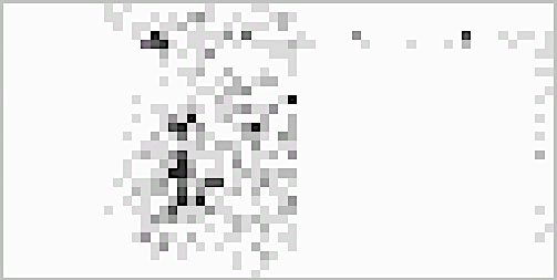
(b) DeRRT^∗

(c) RRT^∗

Figure 2: A test case for the long narrow passage. (a) The DeRRT^∗ search tree, black, and solution, red. (b) A heat map of the DeRRT^∗/HMM search tree. Note the distribution bias toward the channel entrance in the free space, efficient traversal of the channel, and more samples after the channel exit. (c) A heat map of the RRT^∗ search tree. Note the high proportion of time spent looking for the entrance, less efficient traversal of the channel, and few samples in the second free space looking for the goal. Pure black represents allocating 1% of the samples inside the given cell with linear interpolation to pure white.

At test time, we ran each of RRT^∗, DeRRT^∗ with HMMs, and DeRRT^∗ with GRUs for 500 rounds with 600 sampled nodes in each round. DeRRT^∗ was able to succeed far more reliably with such small number of samples, $24\%$ to $47\%$ of the time, a 6 to 12-fold increase, depending on whether the HMMs or the GRUs-based models were used. Table I summarizes the success rate of each planner. We emphasize that the test set is disjoint from the training set both in terms of individual examples but also in terms of the statistics of the examples; the narrower passages required the planners to generalize.

We would like for the algorithms to not just have high performance but also to behave in a directed manner, while still exploring free space. Fig. 2(b) and 2(c) summarize the heat map of the search trees on the given test example. Intensity corresponds to the number of times the tree visited that region. One can see that DeRRT^∗ trades off exploration vs exploitation. It still searches the free space but does so toward the channel entrance, more easily traverses the channel, and samples more densely in the free space after the channel where the goal is.

III-B Bug trap

The bug trap is a standard benchmark in OMPL. It requires that a 2D robot escape from an inner chamber through a narrow passage and then reach a goal in a large free space; see Fig. 3(a). This is made particularly hard by the shape of the exit which includes two dead ends. Most samples in the free space will lead to steering into these areas. For planners to escape from the bug trap, particularly sampling-based planners, a very deliberate sequence of samples must be drawn to guide the robot to the passage and then down the passage without getting trapped.

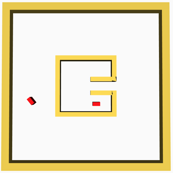
(a) Bug trap

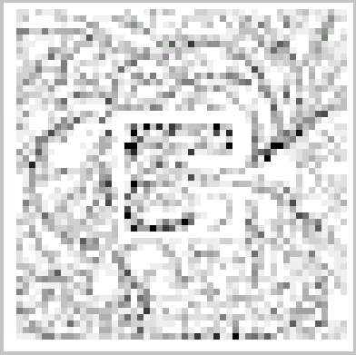
(b) DeRRT^∗

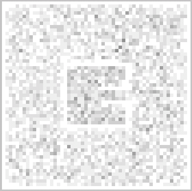
(c) RRT^∗

Figure 3: (a) The default OMPL bug trap example with its start and end position. Note the difficult central passage and dead-ends on either side of it. (b) A heat map of the DeRRT^∗/GRU search tree. It efficiently learns to exit the trap and quickly focuses on sweeping in large arcs to locate the goal. (c) A heat map of the RRT^∗ search tree. It spends more time in the trap and less time on finding the goal in the free space. Pure black represents allocating 0.2% of the samples inside the given cell with linear interpolation to pure white.

Unlike the narrow passage problem, the bug trap has much more distinctive local visual features, i.e., the shape of the trap. To quickly escape, one has to recognize not just the presence of a gap but the particular features of the central channel. In this experiment, we cotrain the convolutional layers of the neural-network sequence models to learn to recognize the presence of relevant map features in order to reach a goal. This eliminates the need for feature engineering or any other annotation aside from a series of prior plans.

To again ensure that the training and test data are disjoint we manipulated the example provided in OMPL. We randomly rotated and translated the trap and randomly sampled the starting position inside the trap and the goal configuration outside the trap. Training samples were provided by running RRT^∗ for 10000 planning steps on each problem instance. In total, we collected 1000 training sequences.

Instead of manually engineering features, we take as an observation $21\times 21$ local patch centered at the current node from a $110\times 110$-sized map. The sequence model used was similar to that from section III-A, with two modifications. First, manually-engineered features were replaced with a two-layer convolutional network, each layer containing a convolution followed by max polling. The convolutions used $3\times 3$ filters with 32 and 64 output channels respectively. Max pooling used a $2\times 2$ window with step size 2. Second, we used GRUs instead of LSTMs as they proved easier to co-train with the convolutional layers.

At test time, we compared RRT^∗ to DeRRT^∗. Fig. 3(a) shows the default bug trap from OMPL. We ensure that the test and training sets are disjoint and that no motion sequence in the training set solves a map from the test set. Each planner is run with a maximum of 10000 planning steps.

Fig. 4 shows the solution length as a function of the number of samples drawn. Already by 4000 samples the sequence-model guided planner is performing as well as RRT^∗ with twice the number of samples. The colored regions show 95% confidence intervals. Additionally, DeRRT^∗ is more stable than RRT^∗, likely because the proportion of valid moves is around 0.8, as shown in Fig. 5. This makes DeRRT^∗ far more efficient in its proposals when compared to RRT^∗. When considering more complex scenarios, such as an articulated robot with a complex mesh, this can have an even more significant impact as the more expensive collision checking can become a dominant concern in the runtime of sampling-based planners.

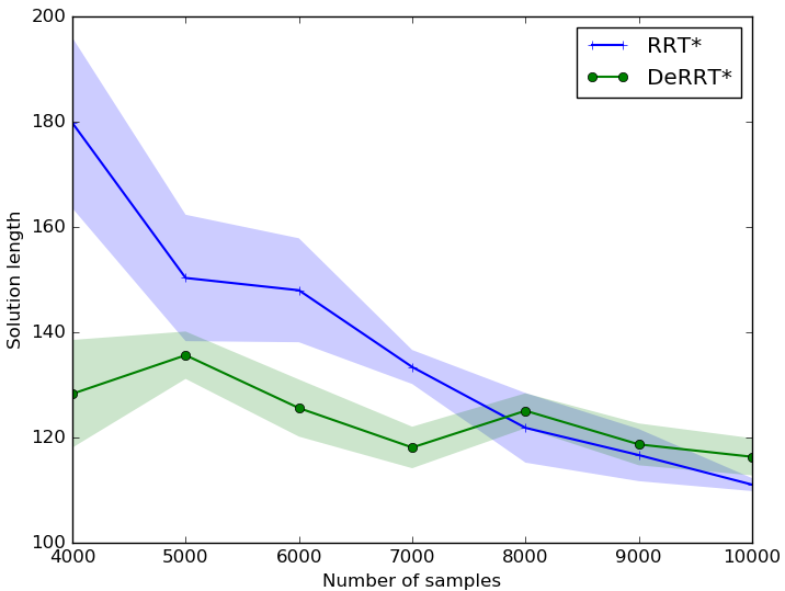
Figure 4: Solution length as a function of the number of samples. DeRRT^∗ is both more efficient and more stable.

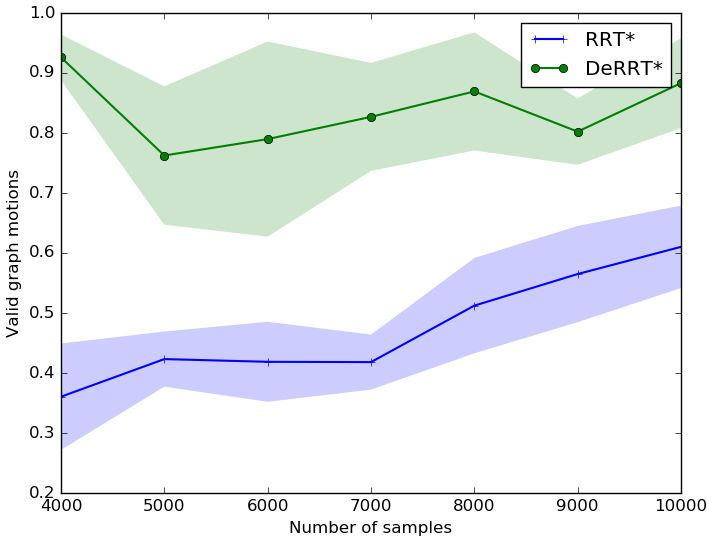
Figure 5: Proportion of valid graph moves as a function of the number of samples. DeRRT^∗ learns to avoid proposing invalid moves.

Figs. 3(b) and  3(c) show heat maps computed the same way as in the previous section where intensity is proportional to the density of nodes. DeRRT^∗ learns to sample less in dead ends and focuses on leaving the channel and exploring the outside space which contains the goal while RRT^∗ tends to spend much more time in the trap.

III-C Multi-agent coordination around a static obstacle

TABLE II: Comparing the success rate and path length as a function of the number of agents of four different planning approaches.

	RRT∗		DeRRT∗/HMM		DeRRT∗/GRU		RRT∗-joint
# of agents	success	path length	success	path length	success	path length	success	path length
2	0.82	$116.74\pm 2.82$	1.00	$112.17\pm 1.42$	1.00	$\phantom{0}96.75\pm 1.01$	0.98	$169.51\pm\phantom{0}9.11$
4	0.68	$122.84\pm 3.46$	0.54	$115.29\pm 2.37$	0.90	$110.88\pm 1.81$	0.46	$302.93\pm 47.82$
6	0.22	$134.30\pm 8.34$	0.30	$111.74\pm 2.22$	0.33	$111.31\pm 1.98$	0.40	$300.79\pm 89.39$
8	0.26	$140.45\pm 6.46$	0.46	$115.27\pm 2.36$	0.18	$108.37\pm 2.05$	0.00	***

Finally, we test the ability of the sequence models to learn to coordinate with other agents using a task where agents must swap their positions around a central obstacle while avoiding each other; see Fig. 7. The obstacle makes the problem significantly harder than a standard position swap in free space since moving randomly in free space makes it very unlikely that agents will collide with each other. To further increase the difficulty, we constrain all other agents to move counter-clockwise around the obstacle. This scenario is closely related to driving; one might view it as a roundabout. To scale the difficulty of the problem, we change the number of agents that must avoid collisions.

Training data was generated by randomly placing an obstacle in a $100\times 100$ map, and up to four agents at random orientation around the obstacle. Motion sequences were supplied by running RRT^∗ for 10,000 iterations. This resulted in 200 different maps and 600 sequences in total. We trained a 3-state HMM including the orientation and distances to the goal and other agents. Similarly to the previous sections, we trained a GRU-based planner including those same features. As described in section II-D, the neural-network-based planner evaluates each of the different agents separately, proposes means and covariance matrices for each, and draws a sample from the resulting mixture model.

We compared DeRRT^∗ to two other approaches, RRT^∗ and RRT^∗-join, with up to eight agents. RRT^∗ only considers the configuration space of the robot while replanning at each step. It treats the map as providing snapshots of fixed obstacles, i.e., the center block and the other agents, some of which happen to move between the snapshots. RRT^∗-joint plans in the joint configuration space of all agents. By reasoning explicitly about the configuration space of other agents, it can in principle take into account the expected trajectories of those agents. Without a model of the behavior of the agents, RRT^∗-joint has difficulties making meaningful inferences aside from constraining the likely paths of other agents to avoid imminent collisions, while at the same time incurring the cost of an exponentially increasing configuration space.

Figure 6: Solution path length in multiagent navigation task

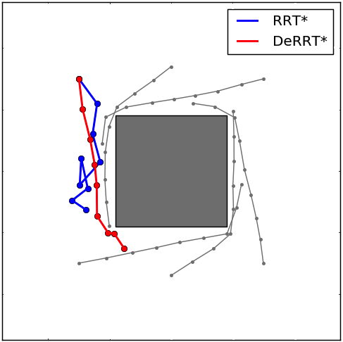
Figure 7: Trajectory comparison in 6 agents swap position case at 500 samples per re-plan step. The grey lines are trajectories of other preloaded agents. (a) Trajectory at the mid-time (b) Trajectory at the end.

Table II shows detailed results comparing these four approaches for a fixed number of samples per re-plan step, 100 for all except for RRT^∗-join which due to its exponentially larger search space requires 5000. RRT^∗-joint quickly degrades because even though it is nominally representing the problem with higher fidelity than RRT^∗, sampling in high dimensional spaces is known to be very difficult. DeRRT^∗ with GRUs performs considerably better in terms of its success rate. Note that DeRRT^∗ was never trained on the same scenarios it was tested on and it was never trained with 6 or 8 agents on the map, yet it seems to generalize well to these new instances. DeRRT^∗ with either sequence model finds much shorter paths. Fig. 6 shows the path length as a function of the number of agents. RRT^∗-joint is omitted because its poor performance would make it difficult to see the difference between any of the other algorithms. As the number of agents increases, DeRRT^∗ does not produce poorer paths, although its likelihood of success does go down as finding collision-free paths becomes more difficult. Figs. 7 and 7 show an instance of this problem along with full tracks, in grey, and partial tracks halfway through the execution, in color, for RRT^∗ and DeRRT^∗ solutions. Even when both approaches reach the goal, the collision-free paths produced by DeRRT^∗ are much smoother.

IV CONCLUSIONS

We have introduced DeRRT^∗, a sampling-based planner extending RRT^∗ with either a graphical model or a neural network in order to learn to plan more efficiently. The algorithm presented here is designed to accommodate a range of sequence models, making minimal assumptions about either the graphical model or the deep network. This opens the door to using models that are successful in other areas, for example, compositional models in vision or sequence-to-sequence models in natural language. We demonstrated how map features can be automatically learned with a CNN and how, when relevant to a planning task, sequence models can learn to predict the motions of other agents leading to more efficient plans. In the future, we expect that planners which understand more about their environments, perhaps by incorporating existing CNNs trained on large vision corpora, will navigate more efficiently. Similarly, sequence models which can capture existing knowledge about an environment and reason about the consequences of actions may be better suited to carrying out complex tasks.

References

- Karaman and Frazzoli [2011] S. Karaman and E. Frazzoli, “Sampling-based algorithms for optimal motion planning,” The International Journal of Robotics Research, vol. 30, no. 7, pp. 846–894, 2011.
- Elbanhawi and Simic [2014] M. Elbanhawi and M. Simic, “Sampling-based robot motion planning: A review,” IEEE Access, 2014.
- Gammell et al. [2015] J. D. Gammell, S. S. Srinivasa, and T. D. Barfoot, “Batch informed trees (BIT∗): Sampling-based optimal planning via the heuristically guided search of implicit random geometric graphs,” in ICRA, 2015.
- Burget et al. [2016] F. Burget, M. Bennewitz, and W. Burgard, “BI2 RRT∗: An efficient sampling-based path planning framework for task-constrained mobile manipulation,” in IROS, 2016.
- Adiyatov and Varol [2017] O. Adiyatov and H. A. Varol, “A novel RRT∗-based algorithm for motion planning in dynamic environments,” in International Conference on Mechatronics and Automation, 2017.
- Urmson and Simmons [2003] C. Urmson and R. Simmons, “Approaches for heuristically biasing RRT growth,” in IROS, 2003.
- Lindemann and LaValle [2004] S. R. Lindemann and S. M. LaValle, “Incrementally reducing dispersion by increasing voronoi bias in RRTs,” in ICRA, 2004.
- Baum and Petrie [1966] L. E. Baum and T. Petrie, “Statistical inference for probabilistic functions of finite state markov chains,” The annals of mathematical statistics, vol. 37, no. 6, pp. 1554–1563, 1966.
- Hochreiter and Schmidhuber [1997] S. Hochreiter and J. Schmidhuber, “Long short-term memory,” Neural computation, vol. 9, no. 8, pp. 1735–1780, 1997.
- Siddharth et al. [2014] N. Siddharth, A. Barbu, and J. Mark Siskind, “Seeing what you’re told: Sentence-guided activity recognition in video,” in CVPR, 2014.
- Yu et al. [2015] H. Yu, N. Siddharth, A. Barbu, and J. M. Siskind, “A compositional framework for grounding language inference, generation, and acquisition in video,” Journal of Artificial Intelligence Research, vol. 52, pp. 601–713, 2015.
- Donahue et al. [2015] J. Donahue, L. Anne Hendricks, S. Guadarrama, M. Rohrbach, S. Venugopalan, K. Saenko, and T. Darrell, “Long-term recurrent convolutional networks for visual recognition and description,” in CVPR, 2015.
- Fulgenzi et al. [2008] C. Fulgenzi, C. Tay, A. Spalanzani, and C. Laugier, “Probabilistic navigation in dynamic environment using rapidly-exploring random trees and gaussian processes,” in IROS, 2008.
- Barbu et al. [2012] A. Barbu, A. Michaux, S. Narayanaswamy, and J. M. Siskind, “Simultaneous object detection, tracking, and event recognition,” Advances in Cognitive Systems, 2012.
- Ramanathan et al. [2016] V. Ramanathan, J. Huang, S. Abu-El-Haija, A. Gorban, K. Murphy, and L. Fei-Fei, “Detecting events and key actors in multi-person videos,” in CVPR, 2016.
- Aoude et al. [2013] G. S. Aoude, B. D. Luders, J. M. Joseph, N. Roy, and J. P. How, “Probabilistically safe motion planning to avoid dynamic obstacles with uncertain motion patterns,” Autonomous Robots, vol. 35, no. 1, pp. 51–76, 2013.
- Le et al. [2017] T. A. Le, A. G. Baydin, and F. Wood, “Inference compilation and universal probabilistic programming,” in Proceedings of the 20th International Conference on Artificial Intelligence and Statistics, 2017.
- Kulkarni et al. [2015] T. D. Kulkarni, P. Kohli, J. B. Tenenbaum, and V. Mansinghka, “Picture: A probabilistic programming language for scene perception,” in CVPR, 2015.
- Narayanaswamy et al. [2012] S. Narayanaswamy, A. Barbu, and J. M. Siskind, “Seeing unseeability to see the unseeable,” Advances in Cognitive Systems, 2012.
- Bowen and Alterovitz [2014] C. Bowen and R. Alterovitz, “Closed-loop global motion planning for reactive execution of learned tasks,” in IROS, 2014.
- Bowen and Alterovitz [2016] ——, “Asymptotically optimal motion planning for tasks using learned virtual landmarks,” IEEE Robotics and Automation Letters, vol. 1, no. 2, pp. 1036–1043, 2016.
- Kim et al. [2018] B. Kim, L. P. Kaelbling, and T. Lozano-Pérez, “Guiding search in continuous state-action spaces by learning an action sampler from off-target search experience,” in AAAI, 2018.
- Goodfellow et al. [2014] I. Goodfellow, J. Pouget-Abadie, M. Mirza, B. Xu, D. Warde-Farley, S. Ozair, A. Courville, and Y. Bengio, “Generative adversarial nets,” in NIPS, 2014.
- Janson et al. [2018] L. Janson, E. Schmerling, and M. Pavone, “Monte carlo motion planning for robot trajectory optimization under uncertainty,” in Robotics Research, 2018, pp. 343–361.
- Arslan et al. [2017] O. Arslan, V. Pacelli, and D. E. Koditschek, “Sensory steering for sampling-based motion planning,” in ICRA, 2017.
- Schmitt et al. [2017] P. S. Schmitt, W. Neubauer, W. Feiten, K. M. Wurm, G. V. Wichert, and W. Burgard, “Optimal, sampling-based manipulation planning,” in ICRA, 2017.
- Čáp et al. [2013] M. Čáp, P. Novák, J. Vokrínek, and M. Pěchouček, “Multi-agent RRT: sampling-based cooperative pathfinding,” in International conference on Autonomous agents and multi-agent systems, 2013.
- Chen et al. [2015] Y. Chen, M. Cutler, and J. P. How, “Decoupled multiagent path planning via incremental sequential convex programming,” in ICRA, 2015.
- Kiesel et al. [2017] S. Kiesel, T. Gu, and W. Ruml, “An effort bias for sampling-based motion planning,” in IROS, 2017.
- Hopfield [1982] J. J. Hopfield, “Neural networks and physical systems with emergent collective computational abilities,” Proceedings of the national academy of sciences, vol. 79, no. 8, pp. 2554–2558, 1982.
- Cho et al. [2014] K. Cho, B. van Merriënboer, D. Bahdanau, and Y. Bengio, “On the properties of neural machine translation: Encoder–decoder approaches,” Syntax, Semantics and Structure in Statistical Translation, p. 103, 2014.
- Palangi et al. [2016] H. Palangi, L. Deng, Y. Shen, J. Gao, X. He, J. Chen, X. Song, and R. Ward, “Deep sentence embedding using long short-term memory networks: Analysis and application to information retrieval,” IEEE/ACM Transactions on Audio, Speech and Language Processing, vol. 24, no. 4, pp. 694–707, 2016.
- Şucan et al. [2012] I. A. Şucan, M. Moll, and L. E. Kavraki, “The Open Motion Planning Library,” IEEE Robotics & Automation Magazine, vol. 19, no. 4, pp. 72–82, December 2012.
- Hsu et al. [1997] D. Hsu, J.-C. Latombe, and R. Motwani, “Path planning in expansive configuration spaces,” in ICRA, 1997.