h KA-TP-28-2018
h PSI-PR-18-10
2HDECAY - A program for the Calculation of Electroweak One-Loop Corrections to Higgs Decays in the Two-Higgs-Doublet Model Including State-of-the-Art QCD Corrections

Abstract

We present the program package 2HDECAY for the calculation of the partial decay widths and branching ratios of the Higgs bosons of a general CP-conserving 2-Higgs doublet model (2HDM). The tool includes the full electroweak one-loop corrections to all two-body on-shell Higgs decays in the 2HDM that are not loop-induced. It combines them with the state-of-the-art QCD corrections that are already implemented in the program HDECAY. For the renormalization of the electroweak sector an on-shell scheme is implemented for most of the renormalization parameters. Exceptions are the soft-$\mathbb{Z}_{2}$-breaking squared mass scale $m_{12}^{2}$, where an $\overline{\text{MS}}$ condition is applied, as well as the 2HDM mixing angles $\alpha$ and $\beta$, for which several different renormalization schemes are implemented. The tool 2HDECAY can be used for phenomenological analyses of the branching ratios of Higgs decays in the 2HDM. Furthermore, the separate output of the electroweak contributions to the tree-level partial decay widths for several different renormalization schemes, computed consistently with an automatic parameter conversion between the different schemes, allows for an efficient analysis of the impact of the electroweak corrections and the remaining theoretical error due to missing higher-order corrections. The latest version of the program package 2HDECAY can be downloaded from the URL https://github.com/marcel-krause/2HDECAY.

1 Introduction

The discovery of the Higgs particle, announced on 4 July 2012 by the LHC experiments ATLAS [1] and CMS [2] marked a milestone for particle physics. It structurally completed the Standard Model (SM) providing us with a theory that remains weakly interacting all the way up to the Planck scale. While the SM can successfully describe numerous particle physics phenomena at the quantum level at highest precision, it leaves open several questions. Among these are e.g. the one for the nature of Dark Matter (DM), the baryon asymmetry of the universe or the hierarchy problem. This calls for physics beyond the SM (BSM). Models beyond the SM usually entail enlarged Higgs sectors that can provide candidates for Dark Matter or guarantee successful baryogenesis. Since the discovered Higgs boson with a mass of 125.09 GeV [3] behaves SM-like any BSM extension has to make sure to contain a Higgs boson in its spectrum that is in accordance with the LHC Higgs data. Moreover, the models have to be tested against theoretical and further experimental constraints from electroweak precision tests, $B$-physics, low-energy observables and the negative searches for new particles that may be predicted by some of the BSM theories.

The lack of any direct sign of new physics renders the investigation of the Higgs sector more and more important. The precise investigation of the discovered Higgs boson may reveal indirect signs of new physics through mixing with other Higgs bosons in the spectrum, loop effects due to the additional Higgs bosons and/or further new states predicted by the model, or decays into non-SM states or Higgs bosons, including the possibility of invisible decays. Due to the SM-like nature of the 125 GeV Higgs boson indirect new physics effects on its properties are expected to be small. Moreover, different BSM theories can lead to similar effects in the Higgs sector. In order not to miss any indirect sign of new physics and to be able to identify the underlying theory in case of discovery, highest precision in the prediction of the observables and sophisticated experimental techniques are therefore indispensable. The former calls for the inclusion of higher-order corrections at highest possible level, and theorists all over the world have spent enormous efforts to improve the predictions for Higgs observables [4].

Among the new physics models supersymmetric (SUSY) extensions [5, 6, 7, 8, 9, 10, 11, 12, 13, 14, 15, 16, 17] certainly belong to the best motivated and most thoroughly investigated models beyond the SM, and numerous higher-order predictions exist for the production and decay cross sections as well as the Higgs potential parameters, i.e. the masses and Higgs self-couplings [4]. The Higgs sector of the minimal supersymmetric extension (MSSM) [17, 18, 19, 20] is a 2-Higgs doublet model (2HDM) of type II [21, 22]. While due to supersymmetry the MSSM Higgs potential parameters are given in terms of gauge couplings this is not the case for general 2HDMs so that the 2HDM entails an interesting and more diverse Higgs phenomenology and is also affected differently by higher-order electroweak (EW) corrections. Moreover, 2HDMs allow for successful baryogenesis [23, 24, 25, 26, 27, 28, 29, 30, 31, 32, 33, 34, 35, 36, 37, 38, 39, 40, 41] and in their inert version provide a Dark Matter candidate [42, 43, 44, 45, 46, 47, 48, 49, 50, 51, 52, 53, 54, 55, 56].

The situation with respect to EW corrections in non-SUSY models is not as advanced as for SUSY extensions. While the QCD corrections can be taken over to those models with a minimum effort from the SM and the MSSM by applying appropriate changes, this is not the case for the EW corrections. Moreover, some issues arise with respect to renormalization. Thus, only recently a renormalization procedure has been proposed by authors of this paper for the mixing angles of the 2HDM that ensures explicitly gauge-independent decay amplitudes, [57, 58]. Subsequent groups have confirmed this in different Higgs channels [59, 60, 61, 62, 63]. Moreover, in Ref. [62] four schemes have been proposed based on on-shell and symmetry-inspired renormalization conditions for the mixing angles (and by applying the background field method [64, 65, 66, 67, 68, 69, 70]) and on $\overline{\mbox{MS}}$ prescriptions for the remaining new quartic Higgs couplings, and their features have been investigated in detail. The authors of Ref. [71] use an improved on-shell scheme that is essentially equivalent to the mixing angle renormalization scheme presented by our group in [57, 58]. It has been applied to compute the renormalized one-loop Higgs boson couplings in the Higgs singlet model and the 2HDM and to implement these in the program H-COUP [72]. In [73] the authors present, for these models, the one-loop electroweak and QCD corrections to the Higgs decays into fermion and gauge boson pairs. The complete phenomenological analysis, however, requires the corrections to all Higgs decays, as we present them here for the first time in the computer tool 2HDECAY.

In [74] we completed the renormalization of the 2HDM and calculated the higher-order corrections to Higgs-to-Higgs decays. We have applied and extended this renormalization procedure in [75] to the next-to-2HDM (N2HDM) which includes an additional real singlet. The computation of the (N)2HDM EW corrections has shown that the corrections can become very large for certain areas of the parameters space. There can be several reasons for this. The corrections can be parametrically enhanced due to involved couplings that can be large [76, 77, 74, 75]. This is in particular the case for the trilinear Higgs self-couplings that in contrast to SUSY are not given in terms of the gauge couplings of the theory and that are so far only weakly constrained by the LHC Higgs data. The corrections can be large due to light particles in the loop in combination with not too small couplings, e.g. light Higgs states of the extended Higgs sector. Also an inapt choice of the renormalization scheme can artificially enhance loop corrections. Thus we found for our investigated processes that process-dependent renormalization schemes or $\overline{\mbox{MS}}$ renormalization of the scalar mixing angles can blow up the one-loop corrections due to an insufficient cancellation of the large finite contributions from wave function renormalization constants [58, 74]. Moreover, counterterms can blow up in certain parameter regions because of small leading-order couplings, e.g. in the 2HDM the coupling of the heavy non-SM-like CP-even Higgs boson to gauge bosons, which in the limit of a light SM-like CP-even Higgs boson is almost zero. The same effects are observed for supersymmetric theories where a badly chosen parameter set for the renormalization can lead to very large counterterms and hence enhanced loop corrections, cf. Ref. [78] for a recent analysis.

This discussion shows that the renormalization of the EW corrections to BSM Higgs observables is a highly non-trivial task. In addition, there may be no unique best renormalization scheme for the whole parameter space of a specific model, and the user has to decide which scheme to choose to obtain trustworthy predictions. With the publication of the new tool 2HDECAY we aim to give an answer to this problematic task.

The program 2HDECAY computes, for 17 different renormalization schemes, the EW corrections to the Higgs decays of the 2HDM Higgs bosons into all possible on-shell two-particle final states of the model that are not loop-induced. It is combined with the widely used Fortran code HDECAY version 6.52 [79, 80] which provides the loop-corrected decay widths and branching ratios for the SM, the MSSM and 2HDM incorporating the state-of-the-art higher-order QCD corrections including also loop-induced and off-shell decays. Through the combination of these corrections with the 2HDM EW corrections 2HDECAY becomes a code for the prediction of the 2HDM Higgs boson decay widths at the presently highest possible level of precision. Additionally, the separate output of the leading order (LO) and next-to-leading order (NLO) EW corrected decay widths allows to perform studies on the importance of the relative EW corrections (as function of the parameter choices), comparisons with the relative EW corrections within the MSSM or investigations on the most suitable renormalization scheme for specific parameter regions. The comparison of the results for different renormalization schemes moreover permits to estimate the remaining theoretical error due to missing higher-order corrections. To that end, 2HDECAY includes a parameter conversion routine which performs the automatic conversion of input parameters from one renormalization scheme to another for all 17 renormalization schemes that are implemented. With this tool we contribute to the effort of improving the theory predictions for BSM Higgs physics observables so that in combination with sophisticated experimental techniques Higgs precision physics becomes possible and the gained insights may advance us in our understanding of the mechanism of electroweak symmetry breaking (EWSB) and the true underlying theory.

The program package was developed and tested under Windows 10, openSUSE Leap 15.0 and macOS Sierra 10.12. It requires an up-to-date version of Python 2 or Python 3 (tested with versions 2.7.14 and 3.5.0), the FORTRAN compiler gfortran and the GNU C compilers gcc (tested for compatibility with versions 6.4.0 and 7.3.1) and g++. The latest version of the package can be downloaded from

https://github.com/marcel-krause/2HDECAY  .

The paper is organized as follows. The subsequent Sec. 2 forms the theoretical background for our work. We briefly introduce the 2HDM, all relevant parameters and particles and set our notation. We give a summary of all counterterms that are needed for the computation of the EW corrections and state them explicitly. The relevant formulae for the computation of the partial decay widths at one-loop level are presented and the combination of the electroweak corrections with the QCD corrections already implemented in HDECAY is described. In Sec. 3, we introduce 2HDECAY in detail, describe the structure of the program package and the input and output file formats. Additionally, we provide installation and usage manuals. We conclude with a short summary of our work in Sec. 4. As reference for the user, we list exemplary input and output files in Appendices A and B, respectively.

2 One-Loop Electroweak and QCD Corrections in the 2HDM

In the following, we briefly set up our notation and introduce the 2HDM along with the input parameters used in our parametrization. We give details on the EW one-loop renormalization of the 2HDM. We discuss how the calculation of the one-loop partial decay widths is performed. At the end of the section, we explain how the EW corrections are combined with the existing state-of-the-art QCD corrections already implemented in HDECAY and present the automatic parameter conversion routine that is implemented in 2HDECAY.

2.1 Introduction of the 2HDM

For our work, we consider a general CP-conserving 2HDM [21, 22] with a global discrete $\mathbb{Z}_{2}$ symmetry that is softly broken. The model consists of two complex $SU(2)_{L}$ doublets $\Phi_{1}$ and $\Phi_{2}$, both with hypercharge $Y=+1$. The electroweak part of the 2HDM can be described by the Lagrangian

$$\mathcal{L}^{\text{EW}}_{\text{2HDM}}=\mathcal{L}_{\text{YM}}+\mathcal{L}_{\text{F}}+\mathcal{L}_{\text{S}}+\mathcal{L}_{\text{Yuk}}+{\mathcal{L}}_{\text{GF}}+\mathcal{L}_{\text{FP}}$$ (2.1)

in terms of the Yang-Mills Lagrangian $\mathcal{L}_{\text{YM}}$ and the fermion Lagrangian $\mathcal{L}_{\text{F}}$ containing the kinetic terms of the gauge bosons and fermions and their interactions, the Higgs Lagrangian $\mathcal{L}_{\text{S}}$, the Yukawa Lagrangian $\mathcal{L}_{\text{yuk}}$ with the Higgs-fermion interactions, the gauge-fixing and the Fadeev-Popov Lagrangian, ${\mathcal{L}}_{\text{GF}}$ and $\mathcal{L}_{\text{FP}}$, respectively. Explicit forms of $\mathcal{L}_{\text{YM}}$ and $\mathcal{L}_{\text{F}}$ can be found e.g. in [81, 82] and of the general 2HDM Yukawa Lagrangian e.g. in [83, 22]. We do not give them explicitly here. For the renormalization of the 2HDM, we follow the approach of Ref. [84] and apply the gauge-fixing only after the renormalization of the theory, i.e. $\mathcal{L}_{\text{GF}}$ contains only fields that are already renormalized. For the purpose of our work we do not present ${\mathcal{L}}_{\text{GF}}$ nor $\mathcal{L}_{\text{FP}}$ since their explicit forms are not needed in the following.

The scalar Lagrangian $\mathcal{L}_{\text{S}}$ introduces the kinetic terms of the Higgs doublets and their scalar potential. With the the covariant derivative

$$D_{\mu}=\partial_{\mu}+\frac{i}{2}g\sum_{a=1}^{3}\sigma^{a}W_{\mu}^{a}+\frac{i}{2}g{{}^{\prime}}B_{\mu}$$ (2.2)

where $W_{\mu}^{a}$ and $B_{\mu}$ are the gauge bosons of the $SU(2)_{L}$ and $U(1)_{Y}$ respectively, $g$ and $g{{}^{\prime}}$ are the corresponding coupling constants of the gauge groups and $\sigma^{a}$ are the Pauli matrices, the scalar Lagrangian is given by

$$\mathcal{L}_{S}=\sum_{i=1}^{2}(D_{\mu}\Phi_{i})^{\dagger}(D^{\mu}\Phi_{i})-V_{\text{2HDM}}~{}.$$ (2.3)

The scalar potential of the CP-conserving 2HDM reads [22]

$$\begin{split}V_{\text{2HDM}}=&~{}m_{11}^{2}\left|\Phi_{1}\right|^{2}+m_{22}^{2}\left|\Phi_{2}\right|^{2}-m_{12}^{2}\left(\Phi_{1}^{\dagger}\Phi_{2}+\textit{h.c.}\right)+\frac{\lambda_{1}}{2}\left(\Phi_{1}^{\dagger}\Phi_{1}\right)^{2}+\frac{\lambda_{2}}{2}\left(\Phi_{2}^{\dagger}\Phi_{2}\right)^{2}\\ &+\lambda_{3}\left(\Phi_{1}^{\dagger}\Phi_{1}\right)\left(\Phi_{2}^{\dagger}\Phi_{2}\right)+\lambda_{4}\left(\Phi_{1}^{\dagger}\Phi_{2}\right)\left(\Phi_{2}^{\dagger}\Phi_{1}\right)+\frac{\lambda_{5}}{2}\left[\left(\Phi_{1}^{\dagger}\Phi_{2}\right)^{2}+\textit{h.c.}\right]~{}.\end{split}$$ (2.4)

Since we consider a CP-conserving model, the 2HDM potential can be parametrized by three real-valued mass parameters $m_{11}$, $m_{22}$ and $m_{12}$ as well as five real-valued dimensionless coupling constants $\lambda_{i}$ ($i=1,...,5$). For later convenience, we define the frequently appearing combination of three of these coupling constants as

$$\lambda_{345}\equiv\lambda_{3}+\lambda_{4}+\lambda_{5}~{}.$$ (2.5)

For $m_{12}^{2}=0$, the potential $V_{\text{2HDM}}$ exhibits a discrete $\mathbb{Z}_{2}$ symmetry under the simultaneous field transformations $\Phi_{1}\rightarrow-\Phi_{1}$ and $\Phi_{2}\rightarrow\Phi_{2}$. This symmetry, implemented in the scalar potential in order to avoid flavour-changing neutral currents (FCNC) at tree level, is softly broken by a non-zero mass parameter $m_{12}$.

After EWSB the neutral components of the Higgs doublets develop vacuum expectation values (VEVs) which are real in the CP-conserving case. After expanding about the real VEVs $v_{1}$ and $v_{2}$, the Higgs doublets $\Phi_{i}$ ($i=1,2$) can be expressed in terms of the charged complex field $\omega_{i}^{+}$ and the real neutral CP-even and CP-odd fields $\rho_{i}$ and $\eta_{i}$, respectively as

$$\Phi_{1}=\begin{pmatrix}\omega^{+}_{1}\\ \frac{v_{1}+\rho_{1}+i\eta_{1}}{\sqrt{2}}\end{pmatrix}~{}~{}~{}\text{and}~{}~{}~{}~{}\Phi_{2}=\begin{pmatrix}\omega^{+}_{2}\\ \frac{v_{2}+\rho_{2}+i\eta_{2}}{\sqrt{2}}\end{pmatrix}$$ (2.6)

where

$$v^{2}=v_{1}^{2}+v_{2}^{2}\approx(246.22~{}\text{GeV})^{2}$$ (2.7)

is the SM VEV obtained from the Fermi constant $G_{F}$ and we define the ratio of the VEVs through the mixing angle $\beta$ as

$$\tan\beta=\frac{v_{2}}{v_{1}}$$ (2.8)

so that

$$v_{1}=vc_{\beta}\quad\mbox{and}\quad v_{2}=vs_{\beta}~{}.$$ (2.9)

Insertion of Eq. (2.6) in the kinetic part of the scalar Lagrangian in Eq. (2.3) yields after rotation to the mass eigenstates the tree-level relations for the masses of the electroweak gauge bosons

$$m_{W}^{2} =\frac{g^{2}v^{2}}{4}$$ (2.10)

$$m_{Z}^{2} =\frac{(g^{2}+g{{}^{\prime}}^{2})v^{2}}{4}$$ (2.11)

$$m_{\gamma}^{2} =0~{}.$$ (2.12)

The electromagnetic coupling constant $e$ is connected to the fine-structure constant $\alpha_{\text{em}}$ and to the gauge boson coupling constants through the tree-level relation

$$e=\sqrt{4\pi\alpha_{\text{em}}}=\frac{gg{{}^{\prime}}}{\sqrt{g^{2}+g{{}^{\prime}}^{2}}}$$ (2.13)

which allows to replace $g{{}^{\prime}}$ in favor of $e$ or $\alpha_{\text{em}}$. In our work, we use the fine-structure constant $\alpha_{\text{em}}$ as an independent input. Alternatively, one could use the tree-level relation to the Fermi constant

$$G_{F}\equiv\frac{\sqrt{2}g^{2}}{8m_{W}^{2}}=\frac{\alpha_{\text{em}}\pi}{\sqrt{2}m_{W}^{2}\left(1-\frac{m_{W}^{2}}{m_{Z}^{2}}\right)}$$ (2.14)

to replace one of the parameters of the electroweak sector in favor of $G_{F}$. Since $G_{F}$ is used as an input value for HDECAY, we present the formula here explicitly and explain the conversion between the different parametrizations in Sec. 2.4.

Inserting Eq. (2.6) in the scalar potential in Eq. (2.4) leads to

$$\begin{split}V_{\text{2HDM}}=&~{}\frac{1}{2}\left(\rho_{1}~{}~{}\rho_{2}\right)M_{\rho}^{2}\begin{pmatrix}\rho_{1}\\ \rho_{2}\end{pmatrix}+\frac{1}{2}\left(\eta_{1}~{}~{}\eta_{2}\right)M_{\eta}^{2}\begin{pmatrix}\eta_{1}\\ \eta_{2}\end{pmatrix}+\frac{1}{2}\left(\omega^{\pm}_{1}~{}~{}\omega^{\pm}_{2}\right)M_{\omega}^{2}\begin{pmatrix}\omega^{\pm}_{1}\\ \omega^{\pm}_{2}\end{pmatrix}\\ &+T_{1}\rho_{1}+T_{2}\rho_{2}+~{}~{}\cdots\end{split}$$ (2.15)

where the terms $T_{1}$ and $T_{2}$ and the matrices $M_{\omega}^{2}$, $M_{\rho}^{2}$ and $M_{\eta}^{2}$ are defined below. By requiring the VEVs of Eq. (2.6) to represent the minimum of the potential, the minimum conditions for the potential can be expressed as

$$\frac{\partial V_{\text{2HDM}}}{\partial\Phi_{i}}\Bigg{|}_{\left\langle\Phi_{j}\right\rangle}=0~{}.$$ (2.16)

This is equivalent to the statement that the two terms linear in the CP-even fields $\rho_{1}$ and $\rho_{2}$, the tadpole terms,

$$\frac{T_{1}}{v_{1}} \equiv m_{11}^{2}-m_{12}^{2}\frac{v_{2}}{v_{1}}+\frac{v_{1}^{2}\lambda_{1}}{2}+\frac{v_{2}^{2}\lambda_{345}}{2}$$ (2.17)

$$\frac{T_{2}}{v_{2}} \equiv m_{22}^{2}-m_{12}^{2}\frac{v_{1}}{v_{2}}+\frac{v_{2}^{2}\lambda_{2}}{2}+\frac{v_{1}^{2}\lambda_{345}}{2}$$ (2.18)

have to vanish at tree level:

$$T_{1}=T_{2}=0~{}~{}~{}(\text{at tree level})~{}.$$ (2.19)

The tadpole equations can be solved for $m_{11}^{2}$ and $m_{22}^{2}$ in order to replace these two parameters by the tadpole parameters $T_{1}$ and $T_{2}$.

The terms bilinear in the fields given in Eq. (2.15) define the scalar mass matrices

$$M_{\rho}^{2} \equiv\begin{pmatrix}m_{12}^{2}\frac{v_{2}}{v_{1}}+\lambda_{1}v_{1}^{2}&-m_{12}^{2}+\lambda_{345}v_{1}v_{2}\\ -m_{12}^{2}+\lambda_{345}v_{1}v_{2}&m_{12}^{2}\frac{v_{1}}{v_{2}}+\lambda_{2}v_{2}^{2}\end{pmatrix}+\begin{pmatrix}\frac{T_{1}}{v_{1}}&0\\ 0&\frac{T_{2}}{v_{2}}\end{pmatrix}$$ (2.20)

$$M_{\eta}^{2} \equiv\left(\frac{m_{12}^{2}}{v_{1}v_{2}}-\lambda_{5}\right)\begin{pmatrix}v_{2}^{2}&-v_{1}v_{2}\\ -v_{1}v_{2}&v_{1}^{2}\end{pmatrix}+\begin{pmatrix}\frac{T_{1}}{v_{1}}&0\\ 0&\frac{T_{2}}{v_{2}}\end{pmatrix}$$ (2.21)

$$M_{\omega}^{2} \equiv\left(\frac{m_{12}^{2}}{v_{1}v_{2}}-\frac{\lambda_{4}+\lambda_{5}}{2}\right)\begin{pmatrix}v_{2}^{2}&-v_{1}v_{2}\\ -v_{1}v_{2}&v_{1}^{2}\end{pmatrix}+\begin{pmatrix}\frac{T_{1}}{v_{1}}&0\\ 0&\frac{T_{2}}{v_{2}}\end{pmatrix}$$ (2.22)

where Eqs. (2.17) and (2.18) have already been applied to replace the parameters $m_{11}^{2}$ and $m_{22}^{2}$ in favor of $T_{1}$ and $T_{2}$. Keeping the latter explicitly in the expressions of the mass matrices is crucial for the correct renormalization of the scalar sector, as explained in Sec. 2.2. By means of two mixing angles $\alpha$ and $\beta$ which define the rotation matrices

$$R(x)\equiv\begin{pmatrix}c_{x}&-s_{x}\\ s_{x}&c_{x}\end{pmatrix}$$ (2.23)

the fields $\omega^{+}_{i}$, $\rho_{i}$ and $\eta_{i}$ are rotated to the mass basis according to

$$\begin{pmatrix}\rho_{1}\\ \rho_{2}\end{pmatrix} =R(\alpha)\begin{pmatrix}H\\ h\end{pmatrix}$$ (2.24)

$$\begin{pmatrix}\eta_{1}\\ \eta_{2}\end{pmatrix} =R(\beta)\begin{pmatrix}G^{0}\\ A\end{pmatrix}$$ (2.25)

$$\begin{pmatrix}\omega^{\pm}_{1}\\ \omega^{\pm}_{2}\end{pmatrix} =R(\beta)\begin{pmatrix}G^{\pm}\\ H^{\pm}\end{pmatrix}$$ (2.26)

with the two CP-even Higgs bosons $h$ and $H$, the CP-odd Higgs boson $A$, the CP-odd Goldstone boson $G^{0}$ and the charged Higgs bosons $H^{\pm}$ as well as the charged Goldstone bosons $G^{\pm}$. In the mass basis, the diagonal mass matrices are given by

$$D_{\rho}^{2} \equiv\begin{pmatrix}m_{H}^{2}&0\\ 0&m_{h}^{2}\end{pmatrix}$$ (2.27)

$$D_{\eta}^{2} \equiv\begin{pmatrix}m_{G^{0}}^{2}&0\\ 0&m_{A}^{2}\end{pmatrix}$$ (2.28)

$$D_{\omega}^{2} \equiv\begin{pmatrix}m_{G^{\pm}}^{2}&0\\ 0&m_{H^{\pm}}^{2}\end{pmatrix}$$ (2.29)

with the diagonal entries representing the squared masses of the respective particles. The Goldstone bosons are massless,

$$m_{G^{0}}^{2}=m_{G^{\pm}}^{2}=0~{}.$$ (2.30)

The squared masses expressed in terms of the potential parameters and the mixing angle $\alpha$ can be cast into the form [77]

$$m_{H}^{2} =c_{\alpha-\beta}^{2}M_{11}^{2}+s_{2(\alpha-\beta)}M_{12}^{2}+s_{\alpha-\beta}^{2}M_{22}^{2}$$ (2.31)

$$m_{h}^{2} =s_{\alpha-\beta}^{2}M_{11}^{2}-s_{2(\alpha-\beta)}M_{12}^{2}+c_{\alpha-\beta}^{2}M_{22}^{2}$$ (2.32)

$$m_{A}^{2} =\frac{m_{12}^{2}}{s_{\beta}c_{\beta}}-v^{2}\lambda_{5}$$ (2.33)

$$m_{H^{\pm}}^{2} =\frac{m_{12}^{2}}{s_{\beta}c_{\beta}}-\frac{v^{2}}{2}\left(\lambda_{4}+\lambda_{5}\right)$$ (2.34)

$$t_{2(\alpha-\beta)} =\frac{2M_{12}^{2}}{M_{11}^{2}-M_{22}^{2}}$$ (2.35)

where we have introduced

$$M_{11}^{2} \equiv v^{2}\left(c_{\beta}^{4}\lambda_{1}+s_{\beta}^{4}\lambda_{2}+2s_{\beta}^{2}c_{\beta}^{2}\lambda_{345}\right)$$ (2.36)

$$M_{12}^{2} \equiv s_{\beta}c_{\beta}v^{2}\left(-c_{\beta}^{2}\lambda_{1}+s_{\beta}^{2}\lambda_{2}+c_{2\beta}\lambda_{345}\right)$$ (2.37)

$$M_{22}^{2} \equiv\frac{m_{12}^{2}}{s_{\beta}c_{\beta}}+\frac{v^{2}}{8}\left(1-c_{4\beta}\right)\left(\lambda_{1}+\lambda_{2}-2\lambda_{345}\right)~{}.$$ (2.38)

Inverting these relations, the quartic couplings $\lambda_{i}$ ($i=1,...,5$) can be expressed in terms of the mass parameters $m_{h}^{2}$, $m_{H}^{2}$, $m_{A}^{2}$, $m_{H^{\pm}}^{2}$ and the CP-even mixing angle $\alpha$ as [77]

$$\lambda_{1} =\frac{1}{v^{2}c_{\beta}^{2}}\left(c_{\alpha}^{2}m_{H}^{2}+s_{\alpha}^{2}m_{h}^{2}-\frac{s_{\beta}}{c_{\beta}}m_{12}^{2}\right)$$ (2.39)

$$\lambda_{2} =\frac{1}{v^{2}s_{\beta}^{2}}\left(s_{\alpha}^{2}m_{H}^{2}+c_{\alpha}^{2}m_{h}^{2}-\frac{c_{\beta}}{s_{\beta}}m_{12}^{2}\right)$$ (2.40)

$$\lambda_{3} =\frac{2m_{H^{\pm}}^{2}}{v^{2}}+\frac{s_{2\alpha}}{s_{2\beta}v^{2}}\left(m_{H}^{2}-m_{h}^{2}\right)-\frac{m_{12}^{2}}{s_{\beta}c_{\beta}v^{2}}$$ (2.41)

$$\lambda_{4} =\frac{1}{v^{2}}\left(m_{A}^{2}-2m_{H^{\pm}}^{2}+\frac{m_{12}^{2}}{s_{\beta}c_{\beta}}\right)$$ (2.42)

$$\lambda_{5} =\frac{1}{v^{2}}\left(\frac{m_{12}^{2}}{s_{\beta}c_{\beta}}-m_{A}^{2}\right)~{}.$$ (2.43)

In order to avoid tree-level FCNC currents, as introduced by the most general 2HDM Yukawa Lagrangian, one type of fermions is allowed to couple only to one Higgs doublet by imposing a global $\mathbb{Z}_{2}$ symmetry under which $\Phi_{1,2}\to\mp\Phi_{1,2}$. Depending on the $\mathbb{Z}_{2}$ charge assignments, there are four phenomenologically different types of 2HDMs summarized in Tab. 1.

	$u$-type	$d$-type	leptons
I	$\Phi_{2}$	$\Phi_{2}$	$\Phi_{2}$
II	$\Phi_{2}$	$\Phi_{1}$	$\Phi_{1}$
lepton-specific	$\Phi_{2}$	$\Phi_{2}$	$\Phi_{1}$
flipped	$\Phi_{2}$	$\Phi_{1}$	$\Phi_{2}$

Table 1: The four Yukawa types of the $\mathbb{Z}_{2}$-symmetric 2HDM defined by the Higgs doublet that couples to each kind of fermions.

For the four 2HDM types considered in this work, all Yukawa couplings can be parametrized through six different Yukawa coupling parameters $Y_{i}$ ($i=1,...,6$) whose values for the different types are presented in Tab. 2. They are introduced here for later convenience.

2HDM type	$Y_{1}$	$Y_{2}$	$Y_{3}$	$Y_{4}$	$Y_{5}$	$Y_{6}$
I	$\frac{c_{\alpha}}{s_{\beta}}$	$\frac{s_{\alpha}}{s_{\beta}}$	$-\frac{1}{t_{\beta}}$	$\frac{c_{\alpha}}{s_{\beta}}$	$\frac{s_{\alpha}}{s_{\beta}}$	$-\frac{1}{t_{\beta}}$
II	$-\frac{s_{\alpha}}{c_{\beta}}$	$\frac{c_{\alpha}}{c_{\beta}}$	$t_{\beta}$	$-\frac{s_{\alpha}}{c_{\beta}}$	$\frac{c_{\alpha}}{c_{\beta}}$	$t_{\beta}$
lepton-specific	$\frac{c_{\alpha}}{s_{\beta}}$	$\frac{s_{\alpha}}{s_{\beta}}$	$-\frac{1}{t_{\beta}}$	$-\frac{s_{\alpha}}{c_{\beta}}$	$\frac{c_{\alpha}}{c_{\beta}}$	$t_{\beta}$
flipped	$-\frac{s_{\alpha}}{c_{\beta}}$	$\frac{c_{\alpha}}{c_{\beta}}$	$t_{\beta}$	$\frac{c_{\alpha}}{s_{\beta}}$	$\frac{s_{\alpha}}{s_{\beta}}$	$-\frac{1}{t_{\beta}}$

Table 2: Parametrization of the Yukawa coupling parameters in terms of six parameters $Y_{i}$ ($i=1,...,6$) for each 2HDM type.

We conclude this section with an overview over the full set of independent parameters that is used as input for the computations in 2HDECAY. Additionally to the parameters defined by ${\mathcal{L}}_{\text{2HDM}}^{\text{EW}}$, HDECAY requires the electromagnetic coupling constant $\alpha_{\text{em}}$ in the Thomson limit for the calculation of the loop-induced decays into a photon pair and into $Z\gamma$, the strong coupling constant $\alpha_{s}$ for the loop-induced decay into gluons and the QCD corrections as well as the total decay widths of the $W$ and $Z$ bosons, $\Gamma_{W}$ and $\Gamma_{Z}$, for the computation of the off-shell decays into massive gauge boson final states. In the mass basis of the scalar sector, the set of independent parameters is given by

$$\{G_{F},\alpha_{s},\Gamma_{W},\Gamma_{Z},\alpha_{\text{em}},m_{W},m_{Z},m_{f},V_{ij},t_{\beta},m_{12}^{2},\alpha,m_{h},m_{H},m_{A},m_{H^{\pm}}\}~{}.$$ (2.44)

Here $m_{f}$ denote the fermion masses of the strange, charm, bottom and top quarks and of the $\mu$ and $\tau$ leptons ($f=s,c,b,t,\mu,\tau$). All other fermion masses are assumed to be zero in HDECAY and will also be assumed to be zero in our computation of the EW corrections to the decay widths. The fermion and gauge boson masses are defined in accordance with the recommendations of the LHC Higgs cross section working group [85]. The $V_{ij}$ denote the CKM mixing matrix elements. All HDECAY decay widths are computed in terms of the Fermi constant $G_{F}$ except for processes involving on-shell external photon vertices that are expressed by $\alpha_{\text{em}}$ in the Thomson limit. In the computation of the EW corrections, however, we require the on-shell masses $m_{W}$ and $m_{Z}$ and the electromagnetic coupling at the $Z$ boson mass scale, $\alpha_{\text{em}}(m_{Z}^{2})$ (not to be confused with the mixing angle $\alpha$ in the Higgs sector), as input parameters for our renormalization conditions. We will come back to this point later.

Alternatively, the original parametrization of the scalar potential in the interaction basis can be used. In this case, the set of independent parameters is given by

$$\{G_{F},\alpha_{s},\Gamma_{W},\Gamma_{Z},\alpha_{\text{em}},m_{W},m_{Z},m_{f},V_{ij},t_{\beta},m_{12}^{2},\lambda_{1},\lambda_{2},\lambda_{3},\lambda_{4},\lambda_{5}\}~{}.$$ (2.45)

However, we want to emphasize that the automatic parameter conversion routine in 2HDECAY is only performed when the parameters are given in the mass basis of Eq. (2.44).

Actually, also the tadpole parameters $T_{1}$ and $T_{2}$ should be included in the two sets as independent parameters of the Higgs potential. However, as described in Sec. 2.2, the treatment of the minimum of the Higgs potential at higher orders requires special care, and in an alternative treatment of the minimum conditions, the tadpole parameters disappear as independent parameters. In any case, after the renormalization procedure is completely performed, the tadpole parameters vanish again and hence, do not count as input parameters for 2HDECAY.

2.2 Renormalization

We focus on the calculation of EW one-loop corrections to decay widths of Higgs particles in the 2HDM. Since the higher-order (HO) corrections of these decay widths are in general ultraviolet (UV)-divergent, a proper regularization and renormalization of the UV divergences is required. In the following, we briefly present the definition of the counterterms (CTs) needed for the calculation of the EW one-loop corrections. For a thorough derivation and presentation of the gauge-independent renormalization of the 2HDM, we refer the reader to [57, 58, 74].

All input parameters that are renormalized for the calculation of the EW corrections (apart from the mixing angles $\alpha$ and $\beta$ and the soft-$\mathbb{Z}_{2}$-breaking scale $m_{12}$) are renormalized in the on-shell (OS) scheme. For the physical fields, we employ the conditions that any mixing of fields with the same quantum numbers shall vanish on the mass shell of the respective particles and that the fields are normalized by fixing the residue of their corresponding propagators at their poles to unity. Mass CTs are fixed through the condition that the masses are defined as the real parts of the poles of the renormalized propagators. These OS conditions suffice to renormalize most of the parameters of the 2HDM necessary for our work. The renormalization of the mixing angles $\alpha$ and $\beta$ follows an OS-motivated approach, as discussed in Sec. 2.2.4, while $m_{12}$ is renormalized via an $\overline{\text{MS}}$ condition as discussed in Sec. 2.2.6.

2.2.1 Renormalization of the Tadpoles

As shown for the 2HDM for the first time in [57, 58], the proper treatment of the tadpole terms at one-loop order is crucial for the gauge-independent definition of the CTs of the mixing angles $\alpha$ and $\beta$. This allows for the calculation of one-loop partial decay widths with a manifestly gauge-independent relation between input variables and the physical observable. In the following, we briefly repeat the different renormalization conditions for the tadpoles that can be employed in the 2HDM.

The standard tadpole scheme is a commonly used renormalization scheme for the tadpoles (cf. e.g. [82] for the SM or [77, 87] for the 2HDM). While the tadpole parameters vanish at tree level, as stated in Eq. (2.19), they are in general non-vanishing at higher orders in perturbation theory. Since the tadpole terms, being the terms linear in the Higgs potential, define the minimum of the potential, it is necessary to employ a renormalization of the tadpoles in such a way that the ground state of the potential still represents the minimum at higher orders. In the standard tadpole scheme, this condition is imposed on the loop-corrected potential. By replacing the tree-level tadpole terms at one-loop order with the physical (i.e. renormalized) tadpole terms and the tadpole CTs $\delta T_{i}$,

$$T_{i}~{}\rightarrow~{}T_{i}+\delta T_{i}~{}~{}~{}(i=1,2)$$ (2.46)

the correct minimum of the loop-corrected potential is obtained by demanding the renormalized tadpole terms $T_{i}$ to vanish. This directly connects the tadpole CTs $\delta T_{i}$ with the corresponding one-loop tadpole diagrams,

$$i\delta T_{H/h}=\mathord{\left(\rule{0.0pt}{30.11249pt}\right.\vbox{ \hbox{ \includegraphics[height=57.21375pt,trim=47.23158pt 34.1433pt 47.23158pt 28.45274pt,clip]{TadpoleDiagramHiggsBasis.pdf} } }\left.\rule{0.0pt}{30.11249pt}\right)}$$ (2.47)

where we switched the tadpole terms from the interaction basis to the mass basis by means of the rotation matrix $R(\alpha)$, as indicated in Eq. (2.24). Since the tadpole terms explicitly appear in the mass matrices in Eqs. (2.20)-(2.22), their CTs explicitly appear in the mass matrices at one-loop order. The rotation from the interaction to the mass basis yields nine tadpole CTs in total which depend on the two tadpole CTs $\delta T_{H/h}$ defined by the one-loop tadpole diagrams in Eq. (2.47): $\displaystyle\delta T_{HH}$ $\displaystyle=\frac{c_{\alpha}^{3}s_{\beta}+s_{\alpha}^{3}c_{\beta}}{vs_{\beta}c_{\beta}}\delta T_{H}-\frac{s_{2\alpha}s_{\beta-\alpha}}{vs_{2\beta}}\delta T_{h}$ (2.48) $\displaystyle\delta T_{Hh}$ $\displaystyle=-\frac{s_{2\alpha}s_{\beta-\alpha}}{vs_{2\beta}}\delta T_{H}+\frac{s_{2\alpha}c_{\beta-\alpha}}{vs_{2\beta}}\delta T_{h}$ (2.49) $\displaystyle\delta T_{hh}$ $\displaystyle=\frac{s_{2\alpha}c_{\beta-\alpha}}{vs_{2\beta}}\delta T_{H}-\frac{s_{\alpha}^{3}s_{\beta}-c_{\alpha}^{3}c_{\beta}}{vs_{\beta}c_{\beta}}\delta T_{h}$ (2.50) $\displaystyle\delta T_{G^{0}G^{0}}$ $\displaystyle=\frac{c_{\beta-\alpha}}{v}\delta T_{H}+\frac{s_{\beta-\alpha}}{v}\delta T_{h}$ (2.51) $\displaystyle\delta T_{G^{0}A}$ $\displaystyle=-\frac{s_{\beta-\alpha}}{v}\delta T_{H}+\frac{c_{\beta-\alpha}}{v}\delta T_{h}$ (2.52) $\displaystyle\delta T_{AA}$ $\displaystyle=\frac{c_{\alpha}s_{\beta}^{3}+s_{\alpha}c_{\beta}^{3}}{vs_{\beta}c_{\beta}}\delta T_{H}-\frac{s_{\alpha}s_{\beta}^{3}-c_{\alpha}c_{\beta}^{3}}{vs_{\beta}c_{\beta}}\delta T_{h}$ (2.53) $\displaystyle\delta T_{G^{\pm}G^{\pm}}$ $\displaystyle=\frac{c_{\beta-\alpha}}{v}\delta T_{H}+\frac{s_{\beta-\alpha}}{v}\delta T_{h}$ (2.54) $\displaystyle\delta T_{G^{\pm}H^{\pm}}$ $\displaystyle=-\frac{s_{\beta-\alpha}}{v}\delta T_{H}+\frac{c_{\beta-\alpha}}{v}\delta T_{h}$ (2.55) $\displaystyle\delta T_{H^{\pm}H^{\pm}}$ $\displaystyle=\frac{c_{\alpha}s_{\beta}^{3}+s_{\alpha}c_{\beta}^{3}}{vs_{\beta}c_{\beta}}\delta T_{H}-\frac{s_{\alpha}s_{\beta}^{3}-c_{\alpha}c_{\beta}^{3}}{vs_{\beta}c_{\beta}}\delta T_{h}$ (2.56) Since the minimum of the potential is defined through the loop-corrected scalar potential, which in general is a gauge-dependent quantity, the CTs defined through this minimum (e.g. the CTs of the scalar or gauge boson masses) become manifestly gauge-dependent themselves. This is no problem as long as all gauge dependences arising in a fixed-order calculation cancel against each other. In the 2HDM, however, an improper renormalization condition for the mixing angle CTs within the standard tadpole scheme can lead to uncanceled gauge dependences in the calculation of partial decay widths. This is discussed in more detail in Sec. 2.2.4. Apart from the appearance of the tadpole diagrams in Eqs. (2.48)-(2.56), and subsequently in the CTs and the wave function renormalization constants (WFRCs) defined through these, the renormalization condition in Eq. (2.47) ensures that all other appearances of tadpoles are canceled in the one-loop calculation, i.e. tadpole diagrams in the self-energies or vertex corrections do not have to be taken into account.

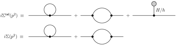
Figure 1: Generic definition of the self-energies $\Sigma$ and $\Sigma^{\text{tad}}$ as function of the external momentum $p^{2}$ used in our CT definitions of the 2HDM. While $\Sigma$ is the textbook definition of the one-particle irreducible self-energy, the self-energy $\Sigma^{\text{tad}}$ additionally contains tadpole diagrams, indicated by the gray blob. For the actual calculation, the full particle content of the 2HDM has to be inserted into the self-energy topologies depicted here.

An alternative treatment of the tadpole renormalization was proposed by J. Fleischer and F. Jegerlehner in the SM [88]. It was applied to the extended scalar sector of the 2HDM for the first time in [57, 58] and is called alternative (FJ) tadpole scheme in the following. In this alternative approach, the VEVs $v_{1,2}$ are considered as the fundamental quantities instead of the tadpole terms. The proper VEVs are the renormalized all-order VEVs of the Higgs fields which represent the true ground state of the theory and which are connected to the particle masses and the couplings of the electroweak sector. Since the alternative approach relies on the minimization of the gauge-independent tree-level scalar potential, the mass CTs defined in this framework become manifestly gauge-independent quantities by themselves. Moreover, the alternative tadpole scheme connects the all-order renormalized VEVs directly to the corresponding tree-level VEVs. Since the tadpoles are not the fundamental quantities of the Higgs minimum in this framework, they do not receive CTs. Instead, CTs for the VEVs are introduced by replacing the VEVs with the renormalized VEVs and their CTs,

$$v_{i}~{}\rightarrow~{}v_{i}+\delta v_{i}$$ (2.57)

and by fixing the latter in such a way that it is ensured that the renormalized VEVs represent the proper tree-level minima to all orders. At one-loop level, this leads to the following connection between the VEV CTs in the interaction basis and the one-loop tadpole diagrams in the mass basis,

$$\delta v_{1}=\frac{-ic_{\alpha}}{m_{H}^{2}}\mathord{\left(\rule{0.0pt}{30.11249pt}\right.\vbox{ \hbox{ \includegraphics[height=57.21375pt,trim=51.21495pt 34.1433pt 49.50777pt 28.45274pt,clip]{TadpoleDiagramHiggsBasisHH.pdf} } }\left.\rule{0.0pt}{30.11249pt}\right)}-\frac{-is_{\alpha}}{m_{h}^{2}}\mathord{\left(\rule{0.0pt}{30.11249pt}\right.\vbox{ \hbox{ \includegraphics[height=57.21375pt,trim=51.21495pt 34.1433pt 49.50777pt 28.45274pt,clip]{TadpoleDiagramHiggsBasish0.pdf} } }\left.\rule{0.0pt}{30.11249pt}\right)}~{}~{}~{}\text{and}~{}~{}~{}\delta v_{2}=\frac{-is_{\alpha}}{m_{H}^{2}}\mathord{\left(\rule{0.0pt}{30.11249pt}\right.\vbox{ \hbox{ \includegraphics[height=57.21375pt,trim=51.21495pt 34.1433pt 49.50777pt 28.45274pt,clip]{TadpoleDiagramHiggsBasisHH.pdf} } }\left.\rule{0.0pt}{30.11249pt}\right)}+\frac{-ic_{\alpha}}{m_{h}^{2}}\mathord{\left(\rule{0.0pt}{30.11249pt}\right.\vbox{ \hbox{ \includegraphics[height=57.21375pt,trim=51.21495pt 34.1433pt 49.50777pt 28.45274pt,clip]{TadpoleDiagramHiggsBasish0.pdf} } }\left.\rule{0.0pt}{30.11249pt}\right)}~{}.$$ (2.58)

The renormalization of the VEVs in the alternative tadpole scheme effectively shifts the VEVs by tadpole contributions. As a consequence, tadpole diagrams have to be considered wherever they can appear in the 2HDM. For the self-energies, this means that the fundamental self-energies used to define the CTs are the ones defined as $\Sigma^{\text{tad}}$ in Fig. 1 instead of the usual one-particle irreducible self-energies $\Sigma$. Additionally, tadpole diagrams have to be considered in the calculation of the one-loop vertex corrections to the Higgs decays. In summary, the renormalization of the tadpoles in the alternative scheme leads to the following conditions:

$\displaystyle\delta T_{ij}$ $\displaystyle=0$ (2.59) $\displaystyle\Sigma(p^{2})~{}$ $\displaystyle\rightarrow~{}\Sigma^{\text{tad}}(p^{2})$ (2.60) Tadpole diagrams have to be considered in the vertex corrections.

2.2.2 Renormalization of the Gauge Sector

For the renormalization of the gauge sector, we introduce CTs and WFRCs for all parameters and fields of the electroweak sector of the 2HDM by applying the shifts

$$m_{W}^{2}~{} \rightarrow~{}m_{W}^{2}+\delta m_{W}^{2}$$ (2.61)

$$m_{Z}^{2}~{} \rightarrow~{}m_{Z}^{2}+\delta m_{Z}^{2}$$ (2.62)

$$\alpha_{\text{em}}~{} \rightarrow~{}\alpha_{\text{em}}+\delta\alpha_{\text{em}}\equiv\alpha_{\text{em}}+2\alpha_{\text{em}}\delta Z_{e}$$ (2.63)

$$W^{\pm}_{\mu}~{} \rightarrow~{}\left(1+\frac{\delta Z_{WW}}{2}\right)W^{\pm}_{\mu}$$ (2.64)

$$\begin{pmatrix}Z\\ \gamma\end{pmatrix}~{} \rightarrow~{}\begin{pmatrix}1+\frac{\delta Z_{ZZ}}{2}&\frac{\delta Z_{Z\gamma}}{2}\\ \frac{\delta Z_{\gamma Z}}{2}&1+\frac{\delta Z_{\gamma\gamma}}{2}\end{pmatrix}\begin{pmatrix}Z\\ \gamma\end{pmatrix}\;$$ (2.65)

where for convenience, we additionally introduced the shift

$$e~{}\rightarrow~{}e\,(1+\delta Z_{e})$$ (2.66)

for the electromagnetic coupling constant by using Eq. (2.13). Applying OS conditions to the gauge sector of the 2HDM leads to equivalent expressions for the CTs as derived in Ref. [82] for the SM, for the standard and alternative tadpole scheme, respectively, $\displaystyle\delta m_{W}^{2}$ $\displaystyle=\textrm{Re}\left[\Sigma_{WW}^{T}\left(m_{W}^{2}\right)\right]$ (2.67) $\displaystyle\delta m_{Z}^{2}$ $\displaystyle=\textrm{Re}\left[\Sigma_{ZZ}^{T}\left(m_{Z}^{2}\right)\right]$ (2.68) $\displaystyle\delta m_{W}^{2}$ $\displaystyle=\textrm{Re}\left[\Sigma_{WW}^{\textrm{tad},T}\left(m_{W}^{2}\right)\right]$ (2.69) $\displaystyle\delta m_{Z}^{2}$ $\displaystyle=\textrm{Re}\left[\Sigma_{ZZ}^{\textrm{tad},T}\left(m_{Z}^{2}\right)\right]$ (2.70) The WFRCs are the same in both tadpole schemes, $\displaystyle\delta Z_{e}(m_{Z}^{2})$ $\displaystyle=\frac{1}{2}\left.\frac{\partial\Sigma^{T}_{\gamma\gamma}\left(p^{2}\right)}{\partial p^{2}}\right|_{p^{2}=0}+\frac{s_{W}}{c_{W}}\frac{\Sigma^{T}_{\gamma Z}\left(0\right)}{m_{Z}^{2}}-\frac{1}{2}\Delta\alpha(m_{Z}^{2})$ (2.71) $\displaystyle\delta Z_{WW}$ $\displaystyle=-\textrm{Re}\left[\frac{\partial\Sigma^{T}_{WW}\left(p^{2}\right)}{\partial p^{2}}\right]_{p^{2}=m_{W}^{2}}$ (2.72) $\displaystyle\begin{pmatrix}\delta Z_{ZZ}&\delta Z_{Z\gamma}\\ \delta Z_{\gamma Z}&\delta Z_{\gamma\gamma}\end{pmatrix}$ $\displaystyle=\begin{pmatrix}-\textrm{Re}\left[\frac{\partial\Sigma^{T}_{ZZ}\left(p^{2}\right)}{\partial p^{2}}\right]_{p^{2}=m_{Z}^{2}}&\frac{2}{m_{Z}^{2}}\Sigma^{T}_{Z\gamma}\left(0\right)\\ -\frac{2}{m_{Z}^{2}}\textrm{Re}\left[\Sigma^{T}_{Z\gamma}\left(m_{Z}^{2}\right)\right]&-\textrm{Re}\left[\frac{\partial\Sigma^{T}_{\gamma\gamma}\left(p^{2}\right)}{\partial p^{2}}\right]_{p^{2}=0}\end{pmatrix}$ (2.73) The superscript $T$ indicates that only the transverse parts of the self-energies are taken into account. The CT for the electromagnetic coupling $\delta Z_{e}(m_{Z}^{2})$ is defined at the scale of the $Z$ boson mass instead of the Thomson limit. For this, the additional term

$$\Delta\alpha(m_{Z}^{2})=\frac{\partial\Sigma_{\gamma\gamma}^{\text{light},T}(p^{2})}{\partial p^{2}}\Bigg{|}_{p^{2}=0}-\frac{\Sigma^{T}_{\gamma\gamma}(m_{Z}^{2})}{m_{Z}^{2}}$$ (2.74)

is required, where the transverse photon self-energy $\Sigma_{\gamma\gamma}^{\text{light},T}(p^{2})$ in Eq. (2.74) contains solely light fermion contributions (i.e. contributions from all fermions apart from the $t$ quark). This ensures that the results of our EW one-loop computations are independent of large logarithms due to light fermion contributions [82].

For later convenience, we additionally introduce the shift of the weak coupling constant

$$g~{}\rightarrow~{}g+\delta g~{}.$$ (2.75)

Since $g$ is not an independent parameter in our approach, cf. Eq. (2.13), the CT $\delta g$ is not independent either and can be expressed through the other CTs derived in this subsection as

$$\frac{\delta g}{g}=\delta Z_{e}(m_{Z}^{2})+\frac{1}{2(m_{Z}^{2}-m_{W}^{2})}\left(\delta m_{W}^{2}-\frac{m_{W}^{2}}{m_{Z}^{2}}\delta m_{Z}^{2}\right)~{}.$$ (2.76)

2.2.3 Renormalization of the Scalar Sector

In the scalar sector of the 2HDM, the masses and fields of the scalar particles are shifted as

$$m_{H}^{2}~{} \rightarrow~{}m_{H}^{2}+\delta m_{H}^{2}$$ (2.77)

$$m_{h}^{2}~{} \rightarrow~{}m_{h}^{2}+\delta m_{h}^{2}$$ (2.78)

$$m_{A}^{2}~{} \rightarrow~{}m_{A}^{2}+\delta m_{A}^{2}$$ (2.79)

$$m_{H^{\pm}}^{2}~{} \rightarrow~{}m_{H^{\pm}}^{2}+\delta m_{H^{\pm}}^{2}$$ (2.80)

$$\begin{pmatrix}H\\ h\end{pmatrix}~{} \rightarrow~{}\begin{pmatrix}1+\frac{\delta Z_{{H}{H}}}{2}&\frac{\delta Z_{{H}{h}}}{2}\\ \frac{\delta Z_{{h}{H}}}{2}&1+\frac{\delta Z_{{h}{h}}}{2}\end{pmatrix}\begin{pmatrix}H\\ h\end{pmatrix}$$ (2.81)

$$\begin{pmatrix}G^{0}\\ A\end{pmatrix}~{} \rightarrow~{}\begin{pmatrix}1+\frac{\delta Z_{{G}^{0}{G}^{0}}}{2}&\frac{\delta Z_{{G}^{0}{A}}}{2}\\ \frac{\delta Z_{{A}{G}^{0}}}{2}&1+\frac{\delta Z_{{A}{A}}}{2}\end{pmatrix}\begin{pmatrix}G^{0}\\ A\end{pmatrix}$$ (2.82)

$$\begin{pmatrix}G^{\pm}\\ H^{\pm}\end{pmatrix}~{} \rightarrow~{}\begin{pmatrix}1+\frac{\delta Z_{{G}^{\pm}{G}^{\pm}}}{2}&\frac{\delta Z_{{G}^{\pm}{H}^{\pm}}}{2}\\ \frac{\delta Z_{{H}^{\pm}{G}^{\pm}}}{2}&1+\frac{\delta Z_{{H}^{\pm}{H}^{\pm}}}{2}\end{pmatrix}\begin{pmatrix}G^{\pm}\\ H^{\pm}\end{pmatrix}~{}.$$ (2.83)

Applying OS renormalization conditions leads to the following CT definitions [57], $\displaystyle\delta Z_{Hh}$ $\displaystyle=\frac{2}{m_{H}^{2}-m_{h}^{2}}\textrm{Re}\Big{[}\Sigma_{Hh}(m_{h}^{2})-\delta T_{Hh}\Big{]}$ (2.84) $\displaystyle\delta Z_{hH}$ $\displaystyle=-\frac{2}{m_{H}^{2}-m_{h}^{2}}\textrm{Re}\Big{[}\Sigma_{Hh}(m_{H}^{2})-\delta T_{Hh}\Big{]}$ (2.85) $\displaystyle\delta Z_{G^{0}A}$ $\displaystyle=-\frac{2}{m_{A}^{2}}\textrm{Re}\Big{[}\Sigma_{G^{0}A}(m_{A}^{2})-\delta T_{G^{0}A}\Big{]}$ (2.86) $\displaystyle\delta Z_{AG^{0}}$ $\displaystyle=\frac{2}{m_{A}^{2}}\textrm{Re}\Big{[}\Sigma_{G^{0}A}(0)-\delta T_{G^{0}A}\Big{]}$ (2.87) $\displaystyle\delta Z_{G^{\pm}H^{\pm}}$ $\displaystyle=-\frac{2}{m_{H^{\pm}}^{2}}\textrm{Re}\Big{[}\Sigma_{G^{\pm}H^{\pm}}(m_{H^{\pm}}^{2})-\delta T_{G^{\pm}H^{\pm}}\Big{]}$ (2.88) $\displaystyle\delta Z_{H^{\pm}G^{\pm}}$ $\displaystyle=\frac{2}{m_{H^{\pm}}^{2}}\textrm{Re}\Big{[}\Sigma_{G^{\pm}H^{\pm}}(0)-\delta T_{G^{\pm}H^{\pm}}\Big{]}$ (2.89) $\displaystyle\delta m_{H}^{2}$ $\displaystyle=\textrm{Re}\Big{[}\Sigma_{HH}(m_{H}^{2})-\delta T_{HH}\Big{]}$ (2.90) $\displaystyle\delta m_{h}^{2}$ $\displaystyle=\textrm{Re}\Big{[}\Sigma_{hh}(m_{h}^{2})-\delta T_{hh}\Big{]}$ (2.91) $\displaystyle\delta m_{A}^{2}$ $\displaystyle=\textrm{Re}\Big{[}\Sigma_{AA}(m_{A}^{2})-\delta T_{AA}\Big{]}$ (2.92) $\displaystyle\delta m_{H^{\pm}}^{2}$ $\displaystyle=\textrm{Re}\Big{[}\Sigma_{H^{\pm}H^{\pm}}(m_{H^{\pm}}^{2})-\delta T_{H^{\pm}H^{\pm}}\Big{]}$ (2.93) $\displaystyle\delta Z_{Hh}$ $\displaystyle=\frac{2}{m_{H}^{2}-m_{h}^{2}}\textrm{Re}\Big{[}\Sigma^{\textrm{tad}}_{Hh}(m_{h}^{2})\Big{]}$ (2.94) $\displaystyle\delta Z_{hH}$ $\displaystyle=-\frac{2}{m_{H}^{2}-m_{h}^{2}}\textrm{Re}\Big{[}\Sigma^{\textrm{tad}}_{Hh}(m_{H}^{2})\Big{]}$ (2.95) $\displaystyle\delta Z_{G^{0}A}$ $\displaystyle=-\frac{2}{m_{A}^{2}}\textrm{Re}\Big{[}\Sigma^{\textrm{tad}}_{G^{0}A}(m_{A}^{2})\Big{]}$ (2.96) $\displaystyle\delta Z_{AG^{0}}$ $\displaystyle=\frac{2}{m_{A}^{2}}\textrm{Re}\Big{[}\Sigma^{\textrm{tad}}_{G^{0}A}(0)\Big{]}$ (2.97) $\displaystyle\delta Z_{G^{\pm}H^{\pm}}$ $\displaystyle=-\frac{2}{m_{H^{\pm}}^{2}}\textrm{Re}\Big{[}\Sigma^{\textrm{tad}}_{G^{\pm}H^{\pm}}(m_{H^{\pm}}^{2})\Big{]}$ (2.98) $\displaystyle\delta Z_{H^{\pm}G^{\pm}}$ $\displaystyle=\frac{2}{m_{H^{\pm}}^{2}}\textrm{Re}\Big{[}\Sigma^{\textrm{tad}}_{G^{\pm}H^{\pm}}(0)\Big{]}$ (2.99) $\displaystyle\delta m_{H}^{2}$ $\displaystyle=\textrm{Re}\Big{[}\Sigma^{\textrm{tad}}_{HH}(m_{H}^{2})\Big{]}$ (2.100) $\displaystyle\delta m_{h}^{2}$ $\displaystyle=\textrm{Re}\Big{[}\Sigma^{\textrm{tad}}_{hh}(m_{h}^{2})\Big{]}$ (2.101) $\displaystyle\delta m_{A}^{2}$ $\displaystyle=\textrm{Re}\Big{[}\Sigma^{\textrm{tad}}_{AA}(m_{A}^{2})\Big{]}$ (2.102) $\displaystyle\delta m_{H^{\pm}}^{2}$ $\displaystyle=\textrm{Re}\Big{[}\Sigma^{\textrm{tad}}_{H^{\pm}H^{\pm}}(m_{H^{\pm}}^{2})\Big{]}$ (2.103) $\displaystyle\delta Z_{HH}$ $\displaystyle=-\textrm{Re}\left[\frac{\partial\Sigma_{HH}\left(p^{2}\right)}{\partial p^{2}}\right]_{p^{2}=m_{H}^{2}}$ (2.104) $\displaystyle\delta Z_{hh}$ $\displaystyle=-\textrm{Re}\left[\frac{\partial\Sigma_{hh}\left(p^{2}\right)}{\partial p^{2}}\right]_{p^{2}=m_{h}^{2}}$ (2.105) $\displaystyle\delta Z_{G^{0}G^{0}}$ $\displaystyle=-\textrm{Re}\left[\frac{\partial\Sigma_{G^{0}G^{0}}\left(p^{2}\right)}{\partial p^{2}}\right]_{p^{2}=0}$ (2.106) $\displaystyle\delta Z_{AA}$ $\displaystyle=-\textrm{Re}\left[\frac{\partial\Sigma_{AA}\left(p^{2}\right)}{\partial p^{2}}\right]_{p^{2}=m_{A}^{2}}$ (2.107) $\displaystyle\delta Z_{G^{\pm}G^{\pm}}$ $\displaystyle=-\textrm{Re}\left[\frac{\partial\Sigma_{G^{\pm}G^{\pm}}\left(p^{2}\right)}{\partial p^{2}}\right]_{p^{2}=0}$ (2.108) $\displaystyle\delta Z_{H^{\pm}H^{\pm}}$ $\displaystyle=-\textrm{Re}\left[\frac{\partial\Sigma_{H^{\pm}H^{\pm}}\left(p^{2}\right)}{\partial p^{2}}\right]_{p^{2}=m_{H^{\pm}}^{2}}$ (2.109) with the tadpole CTs in the standard scheme defined in Eqs. (2.48)-(2.56).

2.2.4 Renormalization of the Scalar Mixing Angles

In the following, we describe the renormalization of the scalar mixing angles $\alpha$ and $\beta$ in the 2HDM. In our approach, we perform the rotation from the interaction to the mass basis, cf. Eqs. (2.24)-(2.26), before renormalization so that the mixing angles need to be renormalized. At one-loop level, the bare mixing angles are replaced by their renormalized values and counterterms as

$$\alpha~{} \rightarrow~{}\alpha+\delta\alpha$$ (2.110)

$$\beta~{} \rightarrow~{}\beta+\delta\beta~{}.$$ (2.111)

The renormalization of the mixing angles in the 2HDM is a non-trivial task and several different schemes have been proposed in the literature. In the following, we only briefly present the definition of the mixing angle CTs in all different schemes that are implemented in 2HDECAY and refer to [57, 58] for details on the derivation of these schemes.

$\overline{\text{MS}}$ scheme. It was shown in [89, 57] that an $\overline{\text{MS}}$ condition for $\delta\alpha$ and $\delta\beta$ can lead to one-loop corrections that are orders of magnitude larger than the LO result. We implemented this scheme in 2HDECAY for reference, as the $\overline{\text{MS}}$ CTs contain only the UV divergences of the CTs, but no finite parts $\left.\delta\alpha\right|_{\text{fin}}$ and $\left.\delta\beta\right|_{\text{fin}}$. After having checked for UV finiteness of the full decay width, the CTs of the mixing angles $\alpha$ and $\beta$ are effectively set to zero in 2HDECAY in this scheme for the numerical evaluation of the partial decay widths. $\displaystyle\left.\delta\alpha\right|_{\text{fin}}$ $\displaystyle=0$ (2.112) $\displaystyle\left.\delta\beta\right|_{\text{fin}}$ $\displaystyle=0$ (2.113) The $\overline{\text{MS}}$ CTs of $\alpha$ and $\beta$ depend on the renormalization scale $\mu_{R}$. The user has to specifiy in the input file the scale at which $\alpha$ and $\beta$ are understood to be given when the $\overline{\text{MS}}$ renormalization scheme is chosen. The one-loop corrected decay widths that contain these CTs, then additionally depend on the renormalization scale of $\alpha$ and $\beta$. The scale at which the decays are evaluated is also defined by the user in the input file and should be chosen appropriately in order to avoid the appearance of large logarithms in the EW one-loop corrections. In case this scale differs from the scale of the $\overline{\text{MS}}$ mixing angles $\alpha$ and $\beta$, the automatic parameter conversion routine converts $\alpha$ and $\beta$ to the scale of the loop-corrected decay widths, as further described in Sec. 2.5. For the conversion, the UV-divergent terms for the CTs $\delta\alpha$ and $\delta\beta$ are needed, i.e. the terms proportional to $1/\varepsilon$. These UV-divergent terms are presented analytically for both the standard and alternative tadpole scheme in Ref. [60]. We cross-checked these terms analytically in an independent calculation.

KOSY scheme. The KOSY scheme (denoted by the authors’ initials) was suggested in [77]. It combines the standard tadpole scheme with the definition of the counterterms through off-diagonal wave function renormalization constants. As shown in [57, 58], the KOSY scheme not only implies a gauge-dependent definition of the mixing angle CTs but also leads to explicitly gauge-dependent decay amplitudes. The CTs are derived by temporarily switching from the mass to the gauge basis. Since $\beta$ diagonalizes both the charged and CP-odd sector not all scalar fields can be defined OS at the same time, unless a systematic modification of the $SU(2)$ relations is performed which we do not do here. We implemented two different CT definitions where $\delta\beta$ is defined through the CP-odd or the charged sectors, indicated by superscripts $o$ and $c$, respectively. The KOSY scheme is implemented in 2HDECAY both in the standard and in the alternative FJ scheme as a benchmark scheme for comparison with other schemes, but for actual computations, we do not recommend to use it due to the explicit gauge dependence of the decay amplitudes. In the KOSY scheme, the mixing angle CTs are defined as $\displaystyle\delta\alpha$ $\displaystyle=\frac{1}{2(m_{H}^{2}-m_{h}^{2})}\text{Re}\left[\Sigma_{Hh}(m_{H}^{2})+\Sigma_{Hh}(m_{h}^{2})-2\delta T_{Hh}\right]$ (2.114) $\displaystyle\delta\beta^{o}$ $\displaystyle=-\frac{1}{2m_{A}^{2}}\text{Re}\left[\Sigma_{G^{0}A}(m_{A}^{2})+\Sigma_{G^{0}A}(0)-2\delta T_{G^{0}A}\right]$ (2.115) $\displaystyle\delta\beta^{c}$ $\displaystyle=-\frac{1}{2m_{H^{\pm}}^{2}}\text{Re}\left[\Sigma_{G^{\pm}H^{\pm}}(m_{H^{\pm}}^{2})+\Sigma_{G^{\pm}H^{\pm}}(0)-2\delta T_{G^{\pm}H^{\pm}}\right]$ (2.116) $\displaystyle\delta\alpha$ $\displaystyle=\frac{1}{2(m_{H}^{2}-m_{h}^{2})}\text{Re}\left[\Sigma^{\text{tad}}_{Hh}(m_{H}^{2})+\Sigma^{\text{tad}}_{Hh}(m_{h}^{2})\right]$ (2.117) $\displaystyle\delta\beta^{o}$ $\displaystyle=-\frac{1}{2m_{A}^{2}}\text{Re}\left[\Sigma^{\text{tad}}_{G^{0}A}(m_{A}^{2})+\Sigma^{\text{tad}}_{G^{0}A}(0)\right]$ (2.118) $\displaystyle\delta\beta^{c}$ $\displaystyle=-\frac{1}{2m_{H^{\pm}}^{2}}\text{Re}\left[\Sigma^{\text{tad}}_{G^{\pm}H^{\pm}}(m_{H^{\pm}}^{2})+\Sigma^{\text{tad}}_{G^{\pm}H^{\pm}}(0)\right]$ (2.119)

$p_{*}$-pinched scheme. One possibility to avoid gauge-parameter-dependent mixing angle CTs was suggested in [57, 58]. The main idea is to maintain the OS-based definition of $\delta\alpha$ and $\delta\beta$ of the KOSY scheme, but instead of using the usual gauge-dependent off-diagonal WFRCs, the WFRCs are defined through pinched self-energies in the alternative FJ scheme by applying the pinch technique (PT) [90, 91, 92, 93, 94, 95, 96, 97]. As worked out for the 2HDM for the first time in [57, 58], the pinched scalar self-energies are equivalent to the usual scalar self-energies in the alternative FJ scheme, evaluated in Feynman-’t Hooft gauge ($\xi=1$), up to additional UV-finite self-energy contributions $\Sigma^{\text{add}}_{ij}(p^{2})$. The mixing angle CTs depend on the scale where the pinched self-energies are evaluated. In the $p_{*}$-pinched scheme, we follow the approach of [98] in the MSSM, where the self-energies $\Sigma^{\text{tad}}_{ij}(p^{2})$ are evaluated at the scale

$$p_{*}^{2}\equiv\frac{m_{i}^{2}+m_{j}^{2}}{2}~{}.$$ (2.120)

At this scale, the additional contributions $\Sigma^{\text{add}}_{ij}(p^{2})$ vanish. Using the $p_{*}$-pinched scheme at one-loop level yields explicitly gauge-parameter-independent partial decay widths. The mixing angle CTs are defined as $\displaystyle\delta\alpha$ $\displaystyle=\frac{1}{m_{H}^{2}-m_{h}^{2}}\text{Re}\left[\Sigma^{\text{tad}}_{Hh}\left(\frac{m_{H}^{2}+m_{h}^{2}}{2}\right)\right]_{\xi=1}$ (2.121) $\displaystyle\delta\beta^{o}$ $\displaystyle=-\frac{1}{m_{A}^{2}}\text{Re}\left[\Sigma^{\text{tad}}_{G^{0}A}\left(\frac{m_{A}^{2}}{2}\right)\right]_{\xi=1}$ (2.122) $\displaystyle\delta\beta^{c}$ $\displaystyle=-\frac{1}{m_{H^{\pm}}^{2}}\text{Re}\left[\Sigma^{\text{tad}}_{G^{\pm}H^{\pm}}\left(\frac{m_{H^{\pm}}^{2}}{2}\right)\right]_{\xi=1}$ (2.123)

OS-pinched scheme. In order to allow for the analysis of the effects of different scale choices of the mixing angle CTs, we implemented another OS-motivated scale choice, which is called the OS-pinched scheme. Here, the additional terms do not vanish and are given by [57]

$$\Sigma^{\textrm{add}}_{Hh}(p^{2}) =\frac{\alpha_{\text{em}}m_{Z}^{2}s_{\beta-\alpha}c_{\beta-\alpha}}{8\pi m_{W}^{2}\left(1-\frac{m_{W}^{2}}{m_{Z}^{2}}\right)}\left(p^{2}-\frac{m_{H}^{2}+m_{h}^{2}}{2}\right)\bigg{\{}\left[B_{0}(p^{2};m_{Z}^{2},m_{A}^{2})-B_{0}(p^{2};m_{Z}^{2},m_{Z}^{2})\right]$$

$$\hskip 11.38092pt+2\frac{m_{W}^{2}}{m_{Z}^{2}}\left[B_{0}(p^{2};m_{W}^{2},m_{H^{\pm}}^{2})-B_{0}(p^{2};m_{W}^{2},m_{W}^{2})\right]\bigg{\}}$$ (2.124)

$$\Sigma^{\textrm{add}}_{G^{0}A}(p^{2}) =\frac{\alpha_{\text{em}}m_{Z}^{2}s_{\beta-\alpha}c_{\beta-\alpha}}{8\pi m_{W}^{2}\left(1-\frac{m_{W}^{2}}{m_{Z}^{2}}\right)}\left(p^{2}-\frac{m_{A}^{2}}{2}\right)\left[B_{0}(p^{2};m_{Z}^{2},m_{H}^{2})-B_{0}(p^{2};m_{Z}^{2},m_{h}^{2})\right]$$ (2.125)

$$\Sigma^{\textrm{add}}_{G^{\pm}H^{\pm}}(p^{2}) =\frac{\alpha_{\text{em}}s_{\beta-\alpha}c_{\beta-\alpha}}{4\pi\left(1-\frac{m_{W}^{2}}{m_{Z}^{2}}\right)}\left(p^{2}-\frac{m_{H^{\pm}}^{2}}{2}\right)\left[B_{0}(p^{2};m_{W}^{2},m_{H}^{2})-B_{0}(p^{2};m_{W}^{2},m_{h}^{2})\right]~{}.$$ (2.126)

The mixing angle CTs in the OS-pinched scheme are then defined as $\displaystyle\delta\alpha$ $\displaystyle=\frac{\textrm{Re}\Big{[}\left[\Sigma^{\textrm{tad}}_{Hh}(m_{H}^{2})+\Sigma^{\textrm{tad}}_{Hh}(m_{h}^{2})\right]_{\xi=1}+\Sigma^{\textrm{add}}_{Hh}(m_{H}^{2})+\Sigma^{\textrm{add}}_{Hh}(m_{h}^{2})\Big{]}}{2\left(m_{H}^{2}-m_{h}^{2}\right)}$ (2.127) $\displaystyle\delta\beta^{o}$ $\displaystyle=-\frac{\textrm{Re}\Big{[}\left[\Sigma^{\textrm{tad}}_{G^{0}A}(m_{A}^{2})+\Sigma^{\textrm{tad}}_{G^{0}A}(0)\right]_{\xi=1}+\Sigma^{\textrm{add}}_{G^{0}A}(m_{A}^{2})+\Sigma^{\textrm{add}}_{G^{0}A}(0)\Big{]}}{2m_{A}^{2}}$ (2.128) $\displaystyle\delta\beta^{c}$ $\displaystyle=-\frac{\textrm{Re}\Big{[}\left[\Sigma^{\textrm{tad}}_{G^{\pm}H^{\pm}}(m_{H^{\pm}}^{2})+\Sigma^{\textrm{tad}}_{G^{\pm}H^{\pm}}(0)\right]_{\xi=1}+\Sigma^{\textrm{add}}_{G^{\pm}H^{\pm}}(m_{H^{\pm}}^{2})+\Sigma^{\textrm{add}}_{G^{\pm}H^{\pm}}(0)\Big{]}}{2m_{H^{\pm}}^{2}}$ (2.129)

Process-dependent schemes. The definition of the mixing angle CTs through observables, like e.g. partial decay widths of Higgs bosons, was proposed for the MSSM in [99, 100] and for the 2HDM in [101]. This scheme leads to explicitly gauge-independent partial decay widths per construction. Moreover, the connection of the mixing angle CTs with physical observables allows for a more physical interpretation of the unphysical mixing angles $\alpha$ and $\beta$. However, as it was shown in [57, 58], process-dependent schemes can in general lead to very large one-loop corrections. We implemented three different process-dependent schemes for $\delta\alpha$ and $\delta\beta$ in 2HDECAY. The schemes differ in the processes that are used for the definition of the CTs. In all cases we have chosen leptonic Higgs boson decays. For these, the QED corrections can be separated in a UV-finite way from the rest of the EW corrections and therefore be excluded from the counterterm definition. This is necessary to avoid the appearance of infrared (IR) divergences in the CTs [100]. The NLO corrections to the partial decay widths of the leptonic decay of a Higgs particle $\phi_{i}$ into a pair of leptons $f_{j}$, $f_{k}$ can then be cast into the form

$$\Gamma_{\phi_{i}f_{j}f_{k}}^{\text{NLO,weak}}=\Gamma_{\phi_{i}f_{j}f_{k}}^{\text{LO}}\left(1+2\text{Re}\left[\mathcal{F}_{\phi_{i}f_{j}f_{k}}^{\text{VC}}+\mathcal{F}_{\phi_{i}f_{j}f_{k}}^{\text{CT}}\right]\right)$$ (2.130)

where $\mathcal{F}_{\phi_{i}f_{j}f_{k}}^{\text{VC}}$ and $\mathcal{F}_{\phi_{i}f_{j}f_{k}}^{\text{CT}}$ are the form factors of the vertex corrections and the CT, respectively, and the superscript weak indicates that in the vertex corrections IR-divergent QED contributions are excluded. The form factor $\mathcal{F}_{\phi_{i}f_{j}f_{k}}^{\text{CT}}$ contains either $\delta\alpha$ or $\delta\beta$ or both simultaneously as well as other CTs that are fixed as described in the other subsections of Sec. 2.2. Employing the renormalization condition

$$\Gamma^{\text{LO}}_{\phi_{i}f_{j}f_{k}}\equiv\Gamma^{\text{NLO,weak}}_{\phi_{i}f_{j}f_{k}}$$ (2.131)

for two different decays then allows for a process-dependent definition of the mixing angle CTs. For more details on the calculation of the CTs in process-dependent schemes in the 2HDM, we refer to [57, 58]. In 2HDECAY, we have chosen the following three different combinations of processes as definition for the CTs,

1. $\delta\beta$ is first defined by $A\rightarrow\tau^{+}\tau^{-}$ and $\delta\alpha$ is subsequently defined by $H\rightarrow\tau^{+}\tau^{-}$.

2. $\delta\beta$ is first defined by $A\rightarrow\tau^{+}\tau^{-}$ and $\delta\alpha$ is subsequently defined by $h\rightarrow\tau^{+}\tau^{-}$.

3. $\delta\beta$ and $\delta\alpha$ are simultaneously defined by $H\rightarrow\tau^{+}\tau^{-}$ and $h\rightarrow\tau^{+}\tau^{-}$.

Employing these renormalization conditions yields the following definitions of the mixing angle CTs: $\displaystyle\delta\alpha$ $\displaystyle=\frac{-Y_{5}}{Y_{4}}\bigg{[}\mathcal{F}^{\textrm{VC}}_{H\tau\tau}+\frac{\delta g}{g}+\frac{\delta m_{\tau}}{m_{\tau}}-\frac{\delta m_{W}^{2}}{2m_{W}^{2}}+Y_{6}\delta\beta+\frac{\delta Z_{HH}}{2}+\frac{Y_{4}}{Y_{5}}\frac{\delta Z_{hH}}{2}+\frac{\delta Z^{\textrm{L}}_{\tau\tau}}{2}$ (2.132) $\displaystyle\hskip 39.83368pt+\frac{\delta Z^{\textrm{R}}_{\tau\tau}}{2}\bigg{]}$ $\displaystyle\delta\beta$ $\displaystyle=\frac{-Y_{6}}{1+Y_{6}^{2}}\bigg{[}\mathcal{F}^{\textrm{VC}}_{A\tau\tau}+\frac{\delta g}{g}+\frac{\delta m_{\tau}}{m_{\tau}}-\frac{\delta m_{W}^{2}}{2m_{W}^{2}}+\frac{\delta Z_{AA}}{2}-\frac{1}{Y_{6}}\frac{\delta Z_{G^{0}A}}{2}+\frac{\delta Z^{\textrm{L}}_{\tau\tau}}{2}+\frac{\delta Z^{\textrm{R}}_{\tau\tau}}{2}\bigg{]}$ (2.133) $\displaystyle\delta\alpha$ $\displaystyle=\frac{Y_{4}}{Y_{5}}\bigg{[}\mathcal{F}^{\textrm{VC}}_{h\tau\tau}+\frac{\delta g}{g}+\frac{\delta m_{\tau}}{m_{\tau}}-\frac{\delta m_{W}^{2}}{2m_{W}^{2}}+Y_{6}\delta\beta+\frac{\delta Z_{hh}}{2}+\frac{Y_{5}}{Y_{4}}\frac{\delta Z_{Hh}}{2}+\frac{\delta Z^{\textrm{L}}_{\tau\tau}}{2}$ (2.134) $\displaystyle\hskip 31.2982pt+\frac{\delta Z^{\textrm{R}}_{\tau\tau}}{2}\bigg{]}$ $\displaystyle\delta\beta$ $\displaystyle=\frac{-Y_{6}}{1+Y_{6}^{2}}\bigg{[}\mathcal{F}^{\textrm{VC}}_{A\tau\tau}+\frac{\delta g}{g}+\frac{\delta m_{\tau}}{m_{\tau}}-\frac{\delta m_{W}^{2}}{2m_{W}^{2}}+\frac{\delta Z_{AA}}{2}-\frac{1}{Y_{6}}\frac{\delta Z_{G^{0}A}}{2}+\frac{\delta Z^{\textrm{L}}_{\tau\tau}}{2}+\frac{\delta Z^{\textrm{R}}_{\tau\tau}}{2}\bigg{]}$ (2.135) $\displaystyle\delta\alpha$ $\displaystyle=\frac{Y_{4}Y_{5}}{Y_{4}^{2}+Y_{5}^{2}}\bigg{[}\mathcal{F}^{\textrm{VC}}_{h\tau\tau}-\mathcal{F}^{\textrm{VC}}_{H\tau\tau}+\frac{\delta Z_{hh}}{2}-\frac{\delta Z_{HH}}{2}+\frac{Y_{5}}{Y_{4}}\frac{\delta Z_{Hh}}{2}-\frac{Y_{4}}{Y_{5}}\frac{\delta Z_{hH}}{2}\bigg{]}$ (2.136) $\displaystyle\delta\beta$ $\displaystyle=\frac{-1}{Y_{6}(Y_{4}^{2}+Y_{5}^{2})}\bigg{[}(Y_{4}^{2}+Y_{5}^{2})\left(\frac{\delta g}{g}+\frac{\delta m_{\tau}}{m_{\tau}}-\frac{\delta m_{W}^{2}}{2m_{W}^{2}}+\frac{\delta Z^{\textrm{L}}_{\tau\tau}}{2}+\frac{\delta Z^{\textrm{R}}_{\tau\tau}}{2}\right)$ (2.137) $\displaystyle\hskip 11.38092pt+Y_{4}Y_{5}\left(\frac{\delta Z_{Hh}}{2}+\frac{\delta Z_{hH}}{2}\right)+Y_{4}^{2}\left(\frac{\delta Z_{hh}}{2}+\mathcal{F}^{\textrm{VC}}_{h\tau\tau}\right)+Y_{5}^{2}\left(\frac{\delta Z_{HH}}{2}+\mathcal{F}^{\textrm{VC}}_{H\tau\tau}\right)\bigg{]}$ Note that for the process-dependent schemes, decays have to be chosen that are experimentally accessible. This may not be the case for certain parameter configurations, in which case the user has to choose, if possible, the decay combination that leads to large enough decay widths to be measurable.

Physical (on-shell) schemes. In order to exploit the advantages of process-dependent schemes, i.e. gauge independence of the mixing angle CTs that are defined within these schemes, while simultaneously avoiding possible drawbacks, e.g. potentially large NLO corrections, the mixing angle CTs can be defined through certain observables or combinations of $S$ matrix elements in such a way that the CTs of all other parameters of the theory do not contribute to the mixing angle CTs. Such a scheme was proposed for the quark mixing within the SM in [102] and for the mixing angle CTs in the 2HDM in [62], where the derivation of the scheme is presented in detail. Here, we only recapitulate the key ideas and state the relevant formulae. For the sole purpose of renormalizing the mixing angles, two right-handed fermion singlets $\nu_{1\text{R}}$ and $\nu_{2\text{R}}$ are added to the 2HDM Lagrangian. An additional discrete $\mathbb{Z}_{2}$ symmetry is imposed under which the singlets transform as

$$\nu_{1\text{R}} \longrightarrow-\nu_{1\text{R}}$$ (2.138)

$$\nu_{2\text{R}} \longrightarrow\nu_{2\text{R}}$$ (2.139)

which prevents lepton generation mixing. The two singlets are coupled via Yukawa couplings $y_{\nu_{1}}$ and $y_{\nu_{2}}$ to two arbitrary left-handed lepton doublets of the 2HDM, giving rise to two massive Dirac neutrinos $\nu_{1}$ and $\nu_{2}$. The CT of the mixing angle $\alpha$ can then be defined by demanding that the ratio of the decay amplitudes of the decays $H\rightarrow\nu_{i}\bar{\nu}_{i}$ and $h\rightarrow\nu_{i}\bar{\nu}_{i}$ (for either $i=1$ or $i=2$) is the same at tree level and at NLO. Taking the ratio of the decay amplitudes has the advantage that other CTs apart from some WFRCs and the mixing angle CTs cancel against each other. For the CT of the mixing angle $\beta$, analogous conditions are imposed, involving additionally the decay of the pseudoscalar Higgs boson $A$ into the pair of massive neutrinos in the ratios of the LO and NLO decay amplitudes. In all cases, the mixing angle CTs are then given as functions of the scalar WFRCs as well as the genuine one-loop vertex corrections to the decays of the scalar particles into the pair of massive neutrinos, namely $\delta_{H\nu_{i}\bar{\nu}_{i}}$, $\delta_{h\nu_{i}\bar{\nu}_{i}}$ and $\delta_{A\nu_{i}\bar{\nu}_{i}}$, as given in Ref. [62]. In this reference, three combinations of ratios of decay amplitudes were chosen to define three different renormalization schemes for the mixing angle CTs in the physical (on-shell) scheme:

• “OS1” scheme: $\mathcal{A}_{H_{1}\rightarrow\nu_{1}\bar{\nu}_{1}}/\mathcal{A}_{H_{2}\rightarrow\nu_{1}\bar{\nu}_{1}}$ for $\delta\alpha$ and $\mathcal{A}_{A\rightarrow\nu_{1}\bar{\nu}_{1}}/\mathcal{A}_{H_{1}\rightarrow\nu_{1}\bar{\nu}_{1}}$ for $\delta\beta$

• “OS2” scheme: $\mathcal{A}_{H_{1}\rightarrow\nu_{2}\bar{\nu}_{2}}/\mathcal{A}_{H_{2}\rightarrow\nu_{2}\bar{\nu}_{2}}$ for $\delta\alpha$ and $\mathcal{A}_{A\rightarrow\nu_{2}\bar{\nu}_{2}}/\mathcal{A}_{H_{1}\rightarrow\nu_{2}\bar{\nu}_{2}}$ for $\delta\beta$

• “OS12” scheme: $\mathcal{A}_{H_{1}\rightarrow\nu_{2}\bar{\nu}_{2}}/\mathcal{A}_{H_{2}\rightarrow\nu_{2}\bar{\nu}_{2}}$ for $\delta\alpha$ and a specific combination of all possible decay amplitudes $\mathcal{A}_{H_{i}\rightarrow\nu_{j}\bar{\nu}_{j}}$ and $\mathcal{A}_{A\rightarrow\nu_{j}\bar{\nu}_{j}}$ ($i,j=1,2$) for $\delta\beta$ .

All three of these schemes were implemented in 2HDECAY^, according to the following definitions of the mixing angle CTs: $\displaystyle\delta\alpha$ $\displaystyle=s_{\alpha}c_{\alpha}\left(\delta_{H\nu_{1}\bar{\nu}_{1}}-\delta_{h\nu_{1}\bar{\nu}_{1}}\right)+s_{\alpha}c_{\alpha}\frac{\delta Z_{HH}-\delta Z_{hh}}{2}+\frac{c_{\alpha}^{2}\delta Z_{Hh}-s_{\alpha}^{2}\delta Z_{hH}}{2}$ (2.140) $\displaystyle\delta\beta$ $\displaystyle=t_{\beta}\Bigg{[}c_{\alpha}^{2}\delta_{H\nu_{1}\bar{\nu}_{1}}+s_{\alpha}^{2}\delta_{h\nu_{1}\bar{\nu}_{1}}-\delta_{A\nu_{1}\bar{\nu}_{1}}+\frac{c_{\alpha}^{2}\delta Z_{HH}+s_{\alpha}^{2}\delta Z_{hh}-\delta Z_{AA}}{2}$ (2.141) $\displaystyle\hskip 35.28157pt-s_{\alpha}c_{\alpha}\frac{\delta Z_{Hh}+\delta Z_{hH}}{2}\Bigg{]}+\frac{\delta Z_{G^{0}A}}{2}$ $\displaystyle\delta\alpha$ $\displaystyle=s_{\alpha}c_{\alpha}\left(\delta_{h\nu_{2}\bar{\nu}_{2}}-\delta_{H\nu_{2}\bar{\nu}_{2}}\right)+s_{\alpha}c_{\alpha}\frac{\delta Z_{hh}-\delta Z_{HH}}{2}+\frac{s_{\alpha}^{2}\delta Z_{Hh}-c_{\alpha}^{2}\delta Z_{hH}}{2}$ (2.142) $\displaystyle\delta\beta$ $\displaystyle=\frac{1}{t_{\beta}}\Bigg{[}\delta_{A\nu_{2}\bar{\nu}_{2}}-s_{\alpha}^{2}\delta_{H\nu_{2}\bar{\nu}_{2}}-c_{\alpha}^{2}\delta_{h\nu_{2}\bar{\nu}_{2}}+\frac{\delta Z_{AA}-s_{\alpha}^{2}\delta Z_{HH}-c_{\alpha}^{2}\delta Z_{hh}}{2}$ (2.143) $\displaystyle\hskip 35.28157pt-s_{\alpha}c_{\alpha}\frac{\delta Z_{Hh}+\delta Z_{hH}}{2}\Bigg{]}+\frac{\delta Z_{G^{0}A}}{2}$ $\displaystyle\delta\alpha$ $\displaystyle=s_{\alpha}c_{\alpha}\left(\delta_{h\nu_{2}\bar{\nu}_{2}}-\delta_{H\nu_{2}\bar{\nu}_{2}}\right)+s_{\alpha}c_{\alpha}\frac{\delta Z_{hh}-\delta Z_{HH}}{2}+\frac{s_{\alpha}^{2}\delta Z_{Hh}-c_{\alpha}^{2}\delta Z_{hH}}{2}$ (2.144) $\displaystyle\delta\beta$ $\displaystyle=s_{\beta}c_{\beta}\left[c_{2\alpha}\frac{\delta Z_{HH}-\delta Z_{hh}}{2}-s_{2\alpha}\frac{\delta Z_{Hh}+\delta Z_{hH}}{2}\right]+\frac{\delta Z_{G^{0}A}}{2}$ (2.145) $\displaystyle\hskip 11.38092pt+s_{\beta}c_{\beta}\left[\delta_{A\nu_{2}\bar{\nu}_{2}}-\delta_{A\nu_{1}\bar{\nu}_{1}}+c_{\alpha}^{2}\delta_{H\nu_{1}\bar{\nu}_{1}}-s_{\alpha}^{2}\delta_{H\nu_{2}\bar{\nu}_{2}}+s_{\alpha}^{2}\delta_{h\nu_{1}\bar{\nu}_{1}}-c_{\alpha}^{2}\delta_{h\nu_{2}\bar{\nu}_{2}}\right]$ For $y_{\nu_{i}}\rightarrow 0$ ($i=1,2$), the two Dirac neutrinos become massless again, the right-handed neutrino singlets decouple and the original 2HDM Lagrangian is recovered. The vertex corrections $\delta_{H\nu_{i}\bar{\nu}_{i}}$, $\delta_{h\nu_{i}\bar{\nu}_{i}}$ and $\delta_{A\nu_{i}\bar{\nu}_{i}}$ are non-vanishing in this limit, however, so that the mixing angle CTs can still be defined through these processes. The mixing angle CTs defined in these physical (on-shell) schemes are manifestly gauge-independent.

Rigid symmetry scheme. The renormalization of mixing matrix elements, e.g. of $\alpha$ and $\beta$ for the scalar sector of the 2HDM, can be connected to the renormalization of the WFRCs by using the rigid symmetry of the Lagrangian. More specifically, it is possible to renormalize the fields and dimensionless parameters of the unbroken gauge theory and to connect the renormalization of the mixing matrix elements of e.g. the scalar sector through a field rotation from the symmetric to the broken phase of the theory. Such a scheme was applied for the renormalization of the SM in [105]. In [62], the scheme was applied to the scalar mixing angles of the 2HDM within the framework of the background field method (BFM) [64, 65, 66, 67, 68, 69, 70], which allows to formulate the mixing angle CTs as functions of the WFRCs $\delta Z_{\hat{H}\hat{h}}$ and $\delta Z_{\hat{h}\hat{H}}$ in the alternative tadpole scheme, where the hat denotes that the fields are given in the BFM framework. These WFRCs differ from the ones used in the non-BFM framework, i.e. $\delta Z_{Hh}$ and $\delta Z_{hH}$ as given by Eqs. (2.94) and (2.95), by some additional term as presented in App. B of [62] which coincides with the additional term given in Eq. (2.124) derived by means of the PT. The scalar self-energies involved in defining the mixing angle CTs are evaluated in a specifically chosen gauge, e.g.  the Feynman-’t Hooft gauge. This leads to the following definition of the CTs according to [62] which is implemented in 2HDECAY, $\displaystyle\delta\alpha$ $\displaystyle=\frac{\textrm{Re}\Big{[}\left[\Sigma^{\textrm{tad}}_{Hh}(m_{H}^{2})+\Sigma^{\textrm{tad}}_{Hh}(m_{h}^{2})\right]_{\xi=1}+\Sigma^{\textrm{add}}_{Hh}(m_{H}^{2})+\Sigma^{\textrm{add}}_{Hh}(m_{h}^{2})\Big{]}}{2\left(m_{H}^{2}-m_{h}^{2}\right)}$ (2.146) $\displaystyle\delta\beta$ $\displaystyle=\frac{s_{2\beta}}{s_{2\alpha}}\frac{\textrm{Re}\Big{[}\left[\Sigma^{\textrm{tad}}_{Hh}(m_{h}^{2})-\Sigma^{\textrm{tad}}_{Hh}(m_{H}^{2})\right]_{\xi=1}+\Sigma^{\textrm{add}}_{Hh}(m_{h}^{2})-\Sigma^{\textrm{add}}_{Hh}(m_{H}^{2})\Big{]}}{2\left(m_{H}^{2}-m_{h}^{2}\right)}$ (2.147) $\displaystyle\hskip 11.38092pt+\frac{e}{2m_{W}\sqrt{1-\frac{m_{W}^{2}}{m_{Z}^{2}}}}\left[s_{\beta-\alpha}\frac{\delta T_{H}}{m_{H}^{2}}-c_{\beta-\alpha}\frac{\delta T_{h}}{m_{h}^{2}}\right]$ where we replaced the BFM WFRCs with the corresponding self-energies and additional terms. As mentioned in [62], we want to remark that the definition of $\delta\alpha$ in the BFMS scheme coincides with the definition in the OS-pinched scheme of Eq. (2.127), while the definition of $\delta\beta$ in the BFMS scheme is different from the one in the OS-pinched scheme.

2.2.5 Renormalization of the Fermion Sector

The masses $m_{f}$, where $f$ generically stands for any fermion of the 2HDM, the CKM matrix elements $V_{ij}$ ($i,j=1,2,3$), the Yukawa coupling parameters $Y_{k}$ ($k=1,...,6)$ and the fields of the fermion sector are replaced by the renormalized quantities and the respective CTs and WFRCs as

$$m_{f}~{} \rightarrow~{}m_{f}+\delta m_{f}$$ (2.148)

$$V_{ij}~{} \rightarrow~{}V_{ij}+\delta V_{ij}$$ (2.149)

$$Y_{k}~{} \rightarrow~{}Y_{k}+\delta Y_{k}$$ (2.150)

$$f_{i}^{L}~{} \rightarrow~{}\left(\delta_{ij}+\frac{\delta Z_{ij}^{f,L}}{2}\right)f_{j}^{L}$$ (2.151)

$$f_{i}^{R}~{} \rightarrow~{}\left(\delta_{ij}+\frac{\delta Z_{ij}^{f,R}}{2}\right)f_{j}^{R}$$ (2.152)

where we use Einstein’s sum convention in the last two lines. The superscripts $L$ and $R$ denote the left- and right-chiral component of the fermion fields, respectively. The Yukawa coupling parameters $Y_{i}$ are not independent input parameters, but functions of $\alpha$ and $\beta$, cf. Tab. 2. Their one-loop counterterms are therefore given in terms of $\delta\alpha$ and $\delta\beta$ defined in Sec. 2.2.4 by the following formulae which are independent of the 2HDM type,

$$\delta Y_{1} =Y_{1}\left(-\frac{Y_{2}}{Y_{1}}\delta\alpha+Y_{3}\delta\beta\right)$$ (2.153)

$$\delta Y_{2} =Y_{2}\left(\frac{Y_{1}}{Y_{2}}\delta\alpha+Y_{3}\delta\beta\right)$$ (2.154)

$$\delta Y_{3} =\left(1+Y_{3}^{2}\right)\delta\beta$$ (2.155)

$$\delta Y_{4} =Y_{4}\left(-\frac{Y_{5}}{Y_{4}}\delta\alpha+Y_{6}\delta\beta\right)$$ (2.156)

$$\delta Y_{5} =Y_{5}\left(\frac{Y_{4}}{Y_{5}}\delta\alpha+Y_{6}\delta\beta\right)$$ (2.157)

$$\delta Y_{6} =\left(1+Y_{6}^{2}\right)\delta\beta~{}.$$ (2.158)

Before presenting the renormalization conditions of the mass CTs and WFRCs, we shortly discuss the renormalization of the CKM matrix. In [82] the renormalization of the CKM matrix is connected to the renormalization of the fields, which in turn are renormalized in an OS approach, leading to the definition ($i,j,k=1,2,3$)

$$\delta V_{ij}=\frac{1}{4}\left[\left(\delta Z^{u,L}_{ik}-\delta Z^{u,L\dagger}_{ik}\right)V_{kj}-V_{ik}\left(\delta Z^{d,L}_{kj}-\delta Z^{d,L\dagger}_{kj}\right)\right]$$ (2.159)

where the superscripts $u$ and $d$ denote up-type and down-type quarks, respectively. This definition of the CKM matrix CTs leads to uncanceled explicit gauge dependences when used in the calculation of EW one-loop corrections, however, [106, 107, 108, 109, 110, 111]. Since the CKM matrix is approximately a unit matrix [112], the numerical effect of this gauge dependence is typically very small, but the definition nevertheless introduces uncanceled explicit gauge dependences into the partial decay widths, which should be avoided. In our work, we follow the approach of Ref. [110] and use pinched fermion self-energies for the definition of the CKM matrix CT. An analytic analysis shows that this is equivalent with defining the CTs in Eq. (2.159) in the Feynman-’t Hooft gauge.

Apart from the CKM matrix CT, all other CTs of the fermion sector are defined through OS conditions. The resulting forms of the CTs are analogous to the ones presented in [82] and given by $\displaystyle\delta m_{f,i}$ $\displaystyle=\frac{m_{f,i}}{2}\text{Re}\left(\Sigma_{ii}^{f,L}(m_{f,i}^{2})+\Sigma_{ii}^{f,R}(m_{f,i}^{2})+2\Sigma_{ii}^{f,S}(m_{f,i}^{2})\right)$ (2.160) $\displaystyle\delta Z^{f,L}_{ij}$ $\displaystyle=\frac{2}{m_{f,i}^{2}-m_{f,j}^{2}}\text{Re}\bigg{[}m_{f,j}^{2}\Sigma_{ij}^{f,L}(m_{f,j}^{2})+m_{f,i}m_{f,j}\Sigma_{ij}^{f,R}(m_{f,j}^{2})$ (2.161) $\displaystyle\hskip 91.04872pt+(m_{f,i}^{2}+m_{f,j}^{2})\Sigma_{ij}^{f,S}(m_{f,j}^{2})\bigg{]}~{}~{}~{}~{}~{}~{}(i\neq j)$ $\displaystyle\delta Z^{f,R}_{ij}$ $\displaystyle=\frac{2}{m_{f,i}^{2}-m_{f,j}^{2}}\text{Re}\bigg{[}m_{f,j}^{2}\Sigma_{ij}^{f,R}(m_{f,j}^{2})+m_{f,i}m_{f,j}\Sigma_{ij}^{f,L}(m_{f,j}^{2})$ (2.162) $\displaystyle\hskip 91.04872pt+2m_{f,i}m_{f,j}\Sigma_{ij}^{f,S}(m_{f,j}^{2})\bigg{]}~{}~{}~{}~{}~{}~{}(i\neq j)$ $\displaystyle\delta m_{f,i}$ $\displaystyle=\frac{m_{f,i}}{2}\text{Re}\left(\Sigma_{ii}^{f,L}(m_{f,i}^{2})+\Sigma_{ii}^{f,R}(m_{f,i}^{2})+2\Sigma_{ii}^{\text{tad},f,S}(m_{f,i}^{2})\right)$ (2.163) $\displaystyle\delta Z^{f,L}_{ij}$ $\displaystyle=\frac{2}{m_{f,i}^{2}-m_{f,j}^{2}}\text{Re}\bigg{[}m_{f,j}^{2}\Sigma_{ij}^{f,L}(m_{f,j}^{2})+m_{f,i}m_{f,j}\Sigma_{ij}^{f,R}(m_{f,j}^{2})$ (2.164) $\displaystyle\hskip 91.04872pt+(m_{f,i}^{2}+m_{f,j}^{2})\Sigma_{ij}^{\text{tad},f,S}(m_{f,j}^{2})\bigg{]}~{}~{}~{}~{}~{}~{}(i\neq j)$ $\displaystyle\delta Z^{f,R}_{ij}$ $\displaystyle=\frac{2}{m_{f,i}^{2}-m_{f,j}^{2}}\text{Re}\bigg{[}m_{f,j}^{2}\Sigma_{ij}^{f,R}(m_{f,j}^{2})+m_{f,i}m_{f,j}\Sigma_{ij}^{f,L}(m_{f,j}^{2})$ (2.165) $\displaystyle\hskip 91.04872pt+2m_{f,i}m_{f,j}\Sigma_{ij}^{\text{tad},f,S}(m_{f,j}^{2})\bigg{]}~{}~{}~{}~{}~{}~{}(i\neq j)$ $\displaystyle\delta V_{ij}$ $\displaystyle=\frac{1}{4}\left[\left(\delta Z^{u,L}_{ik}-\delta Z^{u,L\dagger}_{ik}\right)V_{kj}-V_{ik}\left(\delta Z^{d,L}_{kj}-\delta Z^{d,L\dagger}_{kj}\right)\right]_{\xi=1}$ (2.166) $\displaystyle\delta Z^{f,L}_{ii}$ $\displaystyle=-\textrm{Re}\Big{[}\Sigma^{f,L}_{ii}(m_{f,i}^{2})\Big{]}-m_{f,i}^{2}\textrm{Re}\left[\frac{\partial\Sigma^{f,L}_{ii}(p^{2})}{\partial p^{2}}+\frac{\partial\Sigma^{f,R}_{ii}(p^{2})}{\partial p^{2}}+2\frac{\partial\Sigma^{f,S}_{ii}(p^{2})}{\partial p^{2}}\right]_{p^{2}=m_{f,i}^{2}}$ (2.167) $\displaystyle\delta Z^{f,R}_{ii}$ $\displaystyle=-\textrm{Re}\Big{[}\Sigma^{f,R}_{ii}(m_{f,i}^{2})\Big{]}-m_{f,i}^{2}\textrm{Re}\left[\frac{\partial\Sigma^{f,L}_{ii}(p^{2})}{\partial p^{2}}+\frac{\partial\Sigma^{f,R}_{ii}(p^{2})}{\partial p^{2}}+2\frac{\partial\Sigma^{f,S}_{ii}(p^{2})}{\partial p^{2}}\right]_{p^{2}=m_{f,i}^{2}}$ (2.168) where as before, the superscripts $L$ and $R$ denote the left- and right-chiral parts of the self-energies, while the superscript $S$ denotes the scalar part.

2.2.6 Renormalization of the Soft-$\mathbb{Z}_{2}$-Breaking Parameter $m_{12}^{2}$

The last remaining parameter of the 2HDM that needs to be renormalized is the soft-$\mathbb{Z}_{2}$-breaking parameter $m_{12}^{2}$. As before, we replace the bare parameter by the renormalized one and its corresponding CT,

$$m_{12}^{2}~{}\rightarrow~{}m_{12}^{2}+\delta m_{12}^{2}~{}.$$ (2.169)

In order to fix $\delta m_{12}^{2}$ in a physical way, one could use a process-dependent scheme analogous to Sec. 2.2.4 for the scalar mixing angles. Since $m_{12}^{2}$ only appears in trilinear Higgs couplings, a Higgs-to-Higgs decay width would have to be chosen as observable that fixes the CT. However, as discussed in [74], a process-dependent definition of $\delta m_{12}^{2}$ can lead to very large one-loop corrections in Higgs-to-Higgs decays. We therefore employ an $\overline{\text{MS}}$ condition in 2HDECAY to fix the CT. This is done by calculating the off-shell decay process $h\rightarrow hh$ at one-loop order and by extracting all UV-divergent terms. This fixes the CT of $m_{12}^{2}$ to $\displaystyle\delta m_{12}^{2}$ $\displaystyle=\frac{\alpha_{\text{em}}m_{12}^{2}}{16\pi m_{W}^{2}\left(1-\frac{m_{W}^{2}}{m_{Z}^{2}}\right)}\Big{[}\frac{8m_{12}^{2}}{s_{2\beta}}-2m_{H^{\pm}}^{2}-m_{A}^{2}+\frac{s_{2\alpha}}{s_{2\beta}}(m_{H}^{2}-m_{h}^{2})-3(2m_{W}^{2}+m_{Z}^{2})$ $\displaystyle\hskip 8.5359pt+\sum_{u}3m_{u}^{2}\frac{1}{s_{\beta}^{2}}-\sum_{d}6m_{d}^{2}Y_{3}\left(-Y_{3}-\frac{1}{t_{2\beta}}\right)-\sum_{l}2m_{l}^{2}Y_{6}\left(-Y_{6}-\frac{1}{t_{2\beta}}\right)\Big{]}\Delta$ (2.170) where the sum indices $u$, $d$ and $l$ indicate a summation over all up-type and down-type quarks and charged leptons, respectively, and

$$\Delta\equiv\frac{1}{\varepsilon}-\gamma_{E}+\ln(4\pi)+\ln\left(\frac{\mu^{2}}{\mu_{R}^{2}}\right)~{}.$$ (2.171)

Here, $\gamma_{E}$ is the Euler-Mascheroni constant, $\varepsilon$ the dimensional shift when switching from 4 physical to $D=4-2\varepsilon$ space-time dimensions in the framework of dimensional regularization [113, 114, 115, 116, 117] and $\mu$ is the mass-dimensional ’t Hooft scale which cancels in the calculation of the decay amplitudes. The result in Eq. (2.170) is in agreement with the formula presented in [87]. Since $m_{12}^{2}$ is $\overline{\text{MS}}$ renormalized, the user has to specify in the input file the scale at which the parameter is understood to be given. Just as for the $\overline{\text{MS}}$ renormalized mixing angles, the automatic parameter conversion routine adapts $m_{12}^{2}$ to the scale at which the EW one-loop corrected decay widths are evaluated in case the two scales differ.

2.3 Electroweak Decay Processes at LO and NLO

Figure 2 shows the topologies that contribute to the tree-level and one-loop corrected decay of a scalar particle $\phi$ with four-momentum $p_{1}$ into two other particles $X_{1}$ and $X_{2}$ with four-momenta $p_{2}$ and $p_{3}$, respectively. We emphasize that for the EW corrections, we restrict ourselves to OS decays, i.e. we demand

$$p_{1}^{2}\geq(p_{2}+p_{3})^{2}$$ (2.172)

with $p_{i}^{2}=m_{i}^{2}$ ($i=1,2,3$) where $m_{i}$ denote the masses of the three particles. Moreover, we do not calculate EW corrections to loop-induced Higgs decays, which are of two-loop order. In particular, we do not provide EW corrections to Higgs boson decays into two-gluon, two-photon or $Z\gamma$ final states. Note, however, that the decay widths implemented in HDECAY include also loop-induced decay widths as well as off-shell decays into heavy-quark, massive gauge boson, neutral Higgs pair as well as Higgs and gauge boson final states. We come back to this point in Sec. 2.4.

Figure 2: Decay amplitudes at LO and NLO. The LO decay amplitude $\mathcal{A}^{\text{LO}}_{\phi X_{1}X_{2}}$ simply consists of the trilinear coupling of the three particles $\phi_{1}$, $X_{1}$ and $X_{2}$, while the one-loop amplitude is given by the sum of the genuine vertex corrections $\mathcal{A}^{\text{VC}}_{\phi X_{1}X_{2}}$, indicated by a grey blob, and the vertex counterterm $\mathcal{A}^{\text{CT}}_{\phi X_{1}X_{2}}$ which also includes all WFRCs necessary to render the NLO amplitude UV-finite. We do not show corrections on the external legs since in the decays we consider, they vanish either due to OS renormalization conditions or due to Slavnov-Taylor identities. In the case of the alternative tadpole scheme, the vertex corrections $\mathcal{A}^{\text{VC}}_{\phi X_{1}X_{2}}$ also in general contain tadpole diagrams.

The LO and NLO partial decay widths were calculated by first generating all Feynman diagrams and the corresponding amplitudes for all decay modes that exist for the 2HDM, shown topologically in Fig. 2, with help of the tool FeynArts 3.9 [118]. To that end, we used the 2HDM model file that is implemented in FeynArts, but modified the Yukawa couplings to implement all four 2HDM types. Diagrams that account for NLO corrections on the external legs were not calculated since for all decay modes that we considered, they either vanish due to OS renormalization conditions or due to Slavnov-Taylor identities. All amplitudes were then calculated analytically with FeynCalc 8.2.0 [119, 120], together with all self-energy amplitudes needed for the CTs. For the numerical evaluation of all loop integrals involved in the analytic expression of the one-loop amplitudes, 2HDECAY links LoopTools 2.14 [121].

The LO partial decay width is obtained from the LO amplitude $\mathcal{A}^{\text{LO}}_{\phi X_{1}X_{2}}$, while the NLO amplitude is given by the sum of all amplitudes stemming from the vertex correction and the necessary CTs as defined in Sec. 2.2,

$$\mathcal{A}^{\text{1loop}}_{\phi X_{1}X_{2}}\equiv\mathcal{A}^{\text{VC}}_{\phi X_{1}X_{2}}+\mathcal{A}^{\text{CT}}_{\phi X_{1}X_{2}}~{}.$$ (2.173)

By introducing the Källén phase space function

$$\lambda(x,y,z)\equiv\sqrt{x^{2}+y^{2}+z^{2}-2xy-2xz-2yz}$$ (2.174)

the LO and NLO partial decay widths can be cast into the form

$$\Gamma^{\text{LO}}_{\phi X_{1}X_{2}} =S\frac{\lambda(m_{1}^{2},m_{2}^{2},m_{3}^{2})}{16\pi m_{1}^{3}}\sum_{\text{d.o.f.}}\left|\mathcal{A}_{\phi X_{1}X_{2}}^{\text{LO}}\right|^{2}$$ (2.175)

$$\Gamma^{\text{NLO}}_{\phi X_{1}X_{2}} =\Gamma^{\text{LO}}_{\phi X_{1}X_{2}}+S\frac{\lambda(m_{1}^{2},m_{2}^{2},m_{3}^{2})}{8\pi m_{1}^{3}}\sum_{\text{d.o.f.}}\text{Re}\left[\left(\mathcal{A}_{\phi X_{1}X_{2}}^{\text{LO}}\right)^{*}\mathcal{A}_{\phi X_{1}X_{2}}^{\text{1loop}}\right]+\Gamma_{\phi X_{1}X_{2}+\gamma}$$ (2.176)

where the symmetry factor $S$ accounts for identical particles in the final state and the sum extends over all degrees of freedom of the final-state particles, i.e. over spins or polarizations. The partial decay width $\Gamma_{\phi X_{1}X_{2}+\gamma}$ accounts for real corrections that are necessary for removing IR divergences in all decays that involve charged particles in the initial or final state. For this, we implemented the results given in [122] for generic one-loop two-body partial decay widths. Since the involved integrals are analytically solvable for two-body decays [82], the IR corrections that are implemented in 2HDECAY are given in analytic form as well and do not require numerical integration. Additionally, since the implemented integrals account for the full phase-space of the radiated photon, i.e. both the “hard” and “soft” parts, our results do not depend on arbitrary cuts in the photon phase-space.

In the following, we present all decay channels for which the EW corrections were calculated at one-loop order:

• $h/H/A\to f\bar{f}$   ($f=u,d,c,s,t,b,e,\mu,\tau$)

• $h/H\to VV$   ($V=W^{\pm},Z$)

• $h/H\to VS$   ($V=Z,W^{\pm}$, $S=A,H^{\pm}$)

• $h/H\to SS$   ($S=A,H^{\pm}$)

• $H\to hh$

• $H^{\pm}\to VS$   ($V=W^{\pm}$, $S=h,H,A$)

• $H^{+}\to f\bar{f}$   ($f=u,c,t,\nu_{e},\nu_{\mu},\nu_{\tau}$ , $\bar{f}=\bar{d},\bar{s},\bar{b},e^{+},\mu^{+},\tau^{+}$)

• $A\to VS$   ($V=Z,W^{\pm}$, $S=h,H,H^{\pm}$)

All analytic results of these decay processes are stored in subdirectories of 2HDECAY. For a consistent connection with HDECAY, cf. also Sec. 2.4, not all of these decay processes are used for the calculation of the decay widths and branching ratios, however. Decays containing pairs of first-generation fermions are neglected, i.e. in 2HDECAY, the EW corrections of the following processes are not used for the calculation of the partial decay widths and branching ratios: $h/H/A\to f\bar{f}$ ($f=u,d,e$) and $H^{+}\to f\bar{f}$ ($f\bar{f}=u\bar{d},\nu_{e}e^{+}$). The reason is that they are overwhelmed by the Dalitz decays $\Phi\to f\bar{f}^{(^{\prime})}\gamma$ ($\Phi=h,H,A,H^{\pm}$) that are induced e.g. by off-shell $\gamma^{*}\to f\bar{f}$ splitting.

2.4 Link to HDECAY, Calculated Higher-Order Corrections and Caveats

The EW one-loop corrections to the Higgs decays in the 2HDM derived in this work are combined with HDECAY version 6.52 [79, 80] in form of the new tool 2HDECAY. The Fortran code HDECAY provides the LO and QCD corrected decay widths. As outlined in Sec. 2.2.2 the EW corrections use $\alpha_{\text{em}}$ at the $Z$ boson mass scale as input parameter instead of $G_{F}$ as used in HDECAY. For a consistent combination of the EW corrected decay widths with the HDECAY implementation in the $G_{F}$ scheme we would have to convert between the $\{\alpha_{\text{em}},m_{W},m_{Z}\}$ and the $\{G_{F},m_{W},m_{Z}\}$ scheme including 2HDM higher-order corrections in the conversion formulae. Since these conversion formulae are not implemented yet, we chose a pragmatic approximate solution:

In the configuration of 2HDECAY with OMIT ELW2=0 being set (cf. the input file format described in Sec. 3.5), the EW corrections to the decay widths are calculated automatically. This setting also overwrites the value that the user chooses for the input 2HDM. If e.g. the user does not choose the 2HDM by setting 2HDM=0 but at the same time chooses OMIT ELW2=0 in order to calculate the EW corrections, then a warning is printed and 2HDM=1 is automatically set internally. In this configuration, the value of $G_{F}$ given in the input file of 2HDECAY is ignored by the part of the program that calculates the EW corrections. Instead, $\alpha_{\text{em}}(m_{Z}^{2})$, given in line 26 of the input file, is taken as independent input. This $\alpha_{\text{em}}(m_{Z}^{2})$ is used for the calculation of all electroweak corrections. Subsequently, for the consistent combination with the decay widths of HDECAY computed in terms of the Fermi constant $G_{F}$, the latter decay widths are adapted to the input scheme of the EW corrections by rescaling the HDECAY decay widths with $G_{F}^{\text{calc}}/G_{F}$, where $G_{F}^{\text{calc}}$ is calculated by means of the tree-level relation Eq. (2.14) as a function of $\alpha_{\text{em}}(m_{Z}^{2})$. We expect the differences between the observables within these two schemes to be small.

On the other hand, if OMIT ELW2=1 is set, no EW corrections are computed and 2HDECAY reduces to the original program code HDECAY, including (where applicable) the QCD corrections in the decay widths, the off-shell decays and the loop-induced decays. In this case, the value of $G_{F}$ given in line 27 of the input file is used as input parameter instead of being calculated through the input value of $\alpha_{\text{em}}(m_{Z}^{2})$, and no rescaling with $G_{F}^{\text{calc}}$ is performed. We note in particular that therefore the QCD corrected decay widths, printed out separately by 2HDECAY, will be different in the two input options OMIT ELW2=0 and OMIT ELW2=1.

Another comment is at order in view of the fact that we implemented EW corrections to OS decays only, while HDECAY also features the computation of off-shell decays. More specifically, HDECAY includes off-shell decays into final states with an off-shell top-quark $t^{*}$, i.e. $\phi\to t^{*}\bar{t}$ ($\phi=h,H,A$), $H^{+}\to t^{*}+\bar{d},\bar{s},\bar{b}$, into gauge and Higgs boson final states with an off-shell gauge boson, $h/H\to Z^{*}A,A\to Z^{*}h/H,\phi\to H^{-}W^{+*},H^{+}\to\phi W^{+*}$, and into neutral Higgs pairs with one off-shell Higgs boson that is assumed to predominantly decay into the $b\bar{b}$ final state, $h/H\to AA^{*}$, $H\to hh^{*}$. The top quark total width within the 2HDM, required for the off-shell decays with top final states, is calculated internally in HDECAY. In 2HDECAY, we combine the EW and QCD corrections in such a way that HDECAY still computes the decay widths of off-shell decays, while the electroweak corrections are added only to OS decay channels. It is important to keep this restriction in mind when performing the calculation for large varieties of input data. If e.g. the lighter Higgs boson $h$ is chosen to be the SM-like Higgs boson, then the OS decay $h\rightarrow W^{+}W^{-}$ would be kinematically forbidden while the heavier Higgs boson decay $H\rightarrow W^{+}W^{-}$ might be OS. In such cases, 2HDECAY calculates the EW NLO corrections only for the latter decay channel, while the LO (and QCD decay widths where applicable) are calculated for both. The same is true for any other decay channel for which we implemented EW corrections but which are off-shell in certain input scenarios. Note, that the NLO EW corrections for the off-shell decays into the massive gauge boson final states have been provided for the 2HDM in [60, 62, 61]. For the SM, the combination of HDECAY and Prophecy4f [123, 124, 125] provides the decay widths including EW corrected off-shell decays into these final states. In a similar way, a combination of 2HDECAY and Prophecy4f with the 2HDM decays may be envisaged in future.

For the combination of the QCD and EW corrections finally, we assume that these corrections factorize. We denote by $\delta^{\text{QCD}}$ and $\delta^{\text{EW}}$ the relative QCD and EW corrections, respectively. Here $\delta^{\text{QCD}}$ is normalized to the LO width $\Gamma^{\text{HD,LO}}$, calculated internally by HDECAY. This means for example in the case of quark pair final states that the LO width includes the running quark mass in order to improve the perturbative behaviour. The relative EW corrections $\delta^{\text{EW}}$ on the other hand are obtained by normalization to the LO width with on-shell particle masses. With these definitions the QCD and EW corrected decay width into a specific final state, $\Gamma^{\text{QCD\&EW}}$, is given by

$$\Gamma^{\text{QCD\&EW}}=\frac{G_{F}^{\text{calc}}}{G_{F}}\Gamma^{\text{HD,LO}}[1+\delta^{\text{QCD}}][1++\delta^{\text{EW}}]\equiv\frac{G_{F}^{\text{calc}}}{G_{F}}\Gamma^{\text{HD,QCD}}[1+\delta^{\text{EW}}]\;.$$ (2.177)

We have included the rescaling factor $G_{F}^{\text{calc}}/G_{F}$ which is necessary for the consistent connection of our EW corrections with the decay widths obtained from HDECAY, as outline above.

QCD&EW-corrected branching ratios: The program code will provide the branching ratios calculated originally by HDECAY, which, however, for OMIT ELW2=0 are rescaled by $G_{F}^{\text{calc}}/G_{F}$. They include all loop decays, off-shell decays and QCD corrections where applicable. We summarize these branching ratios under the name ’QCD-corrected’ branching ratios and call their associated decay widths $\Gamma^{\text{HD,QCD}}$, keeping in mind that the QCD corrections are included only where applicable. Furthermore, the EW and QCD corrected branching ratios will be given out. Here, we add the EW corrections to the decay widths calculated internally by HDECAY where possible, i.e. for non-loop induced and OS decay widths. We summarize these branching ratios under the name ’QCD&EW-corrected’ branching ratios and call their associated decay widths $\Gamma^{\text{QCD\&EW}}$. In Table 3 we summarize all details and caveats on their calculation that we described here above. All these branching ratios are written to the output file carrying the suffix ’_BR’ with its filename, see also end of section 3.5 for details.

IELW2=0	QCD-corrected	QCD&EW-corrected
on-shell and	$\Gamma^{\text{HD,QCD}}\frac{G_{F}^{\text{calc}}}{G_{F}}$	$\Gamma^{\text{HD,QCD}}[1+\delta^{\text{EW}}]\frac{G_{F}^{\text{calc}}}{G_{F}}$
non-loop induced
off-shell or	$\Gamma^{\text{HD,QCD}}\frac{G_{F}^{\text{calc}}}{G_{F}}$	$\Gamma^{\text{HD,QCD}}\frac{G_{F}^{\text{calc}}}{G_{F}}$
loop-induced

Table 3: The QCD-corrected and the QCD&EW-corrected decay widths as calculated by 2HDECAY for IELW2=0. The label QCD is in the sense that the QCD corrections are included where applicable.

NLO EW-corrected decay widths: For ${\tt IELW2=0}$, we additionally give out the LO and the EW-corrected NLO decay widths as calculated by the new addition to HDECAY. Here the LO widths do not include any running of the quark masses in the case of quark final states, but are obtained for OS masses. They can hence differ quite substantially from the LO widths as calculated in the original HDECAY version. These LO and EW-corrected NLO widths are computed in the $\{\alpha_{\text{em}},m_{W},m_{Z}\}$ scheme and therefore obviously do not need the inclusion of the rescaling factor $G_{F}^{\text{calc}}/G_{F}$. The decay widths are written to the output file carrying the suffix ’_EW’ with its filename. While the widths given out here are not meant to be applied in Higgs observables as they do not include the important QCD corrections, the study of the NLO EW-corrected decay widths for various renormalization schemes, as provided by 2HDECAY, allows to analyze the importance of the EW corrections and estimate the remaining theoretical error due to missing higher-order EW corrections. The decay widths can also be used for phenomenological studies like e.g. the comparison with the EW-corrected decay widths in the MSSM in the limit of large supersymmetric particle masses, or the investigation of specific 2HDM parameter regions at LO and NLO as e.g. the alignment limit, the non-decoupling limit or the wrong-sign limit.

Caveats: We would like to point out to the user that it can happen that the EW-corrected decay widths become negative because of too large negative EW corrections compared to the LO width. There can be several reasons for this: $(i)$ The LO width may be very small in parts of the parameter space due to suppressed couplings. For example the decay of the heavy Higgs boson $H$ into massive vector bosons is very small in the region where the lighter $h$ becomes SM-like and takes over almost the whole coupling to massive gauge bosons. If the NLO EW width is not suppressed by the same power of the relevant coupling or if at NLO there are cancellations between the various terms that remove the suppression, the NLO width can largely exceed the LO width. $(ii)$ The EW corrections are artificially enhanced due to a badly chosen renormalization scheme, cf. Refs. [58, 74, 75] for investigations on this subject. The choice of a different renormalization scheme may cure this problem, but of course raises also the question for the remaining theoretical error due to missing higher-order corrections. $(iii)$ The EW corrections are parametrically enhanced due to involved couplings that are large, because of small coupling parameters in the denominator or due to light particles in the loop, see also Refs. [58, 74, 75] for discussions. This would call for the resummation of EW corrections beyond NLO to improve the behaviour. It is obvious that the EW corrections should not be trusted in case of extremely large positive or negative corrections and rather be discarded, in particular in the comparison with experimental observables, unless some of the suggested measures are taken to improve the behaviour.

2.5 Parameter Conversion

Through the higher-order corrections the decay widths depend on the renormalization scale. In 2HDECAY the user can choose this scale, called $\mu_{\text{out}}$ in the following, in the input file. It can either chosen to be a fixed scale or the mass of the decaying Higgs boson. Input parameters in the $\overline{\mbox{MS}}$ scheme depend explicitly on the renormalization scale $\mu_{R}$. This scale also has to be given by the user in the input scale, and is called $\mu_{R}$ in the following. The value of the scale becomes particularly important when the values of $\mu_{R}$ and $\mu_{\text{out}}$ differ. In this case the $\overline{\mbox{MS}}$ parameters have to be evolved from the scale $\mu_{R}$ to the scale $\mu_{\text{out}}$. This applies for $m_{12}^{2}$ which is always understood to be an $\overline{\mbox{MS}}$ parameter, and for $\alpha$ and $\beta$ in case they are chosen to be $\overline{\mbox{MS}}$ renormalized. 2HDECAY internally converts the $\overline{\mbox{MS}}$ parameters from $\mu_{R}$ to $\mu_{\text{out}}$ by means of a linear approximation, applying the formula

$$\varphi\left(\{\mu_{\text{out}}\}\right)\approx\varphi\left(\{\mu_{R}\}\right)+\ln\left(\frac{\mu_{\text{out}}^{2}}{\mu_{R}^{2}}\right)\delta\varphi^{\text{div}}\left(\{\varphi\}\right)$$ (2.178)

where $\varphi$ and $\delta\varphi$ denote the $\overline{\mbox{MS}}$ parameters ($\alpha$ and $\beta$, if chosen as such, $m_{12}^{2}$) and their respective counterterms. The index ’div’ means that only the divergent part of the counterterm, i.e. the terms proportional to $1/\varepsilon$ (or equivalently $\Delta$), is taken.

In addition, a parameter conversion has to be performed, when the chosen renormalization scheme of the input parameter differs from the renormalization scheme at which the EW corrected decay widths are chosen to be evaluated. 2HDECAY performs this conversion automatically which is necessary for a consistent interpretation of the results. The renormalization schemes implemented in 2HDECAY differ solely in their definition of the scalar mixing angle CTs, while the defnition of all other CTs is fixed. Therefore, the values of $\alpha$ and $\beta$ must be converted when switching from one renormalization scheme to another. For this conversion, we follow the linearized approach described in Ref. [60]. Since the bare mixing angles are independent of the renormalization scheme, their values $\varphi_{i}$ in a different renormalization scheme are given by the values $\varphi_{\text{ref}}$ in the input scheme (called reference scheme in the following) and the corresponding counterterms $\delta\varphi_{\text{ref}}$ and $\delta\varphi_{i}$ in the reference and the other renormalization scheme, respectively, as

$$\varphi_{i}\left(\{\mu_{\text{out}}\}\right)\approx\varphi_{\text{ref}}\left(\{\mu_{R}\}\right)+\delta\varphi_{\text{ref}}\left(\{\varphi_{\text{ref}},\mu_{R}\}\right)-\delta\varphi_{i}\left(\{\varphi_{\text{ref}},\mu_{\text{out}}\}\right)~{}.$$ (2.179)

Note, that Eq. (2.179) also contains the dependence on the scales $\mu_{R}$ and $\mu_{\text{out}}$ introduced above. They are relevant in case $\alpha$ and $\beta$ are understood as $\overline{\mbox{MS}}$ parameters and additionally depend on the renormalization scale, at which they are defined. The relation Eq. (2.179) holds approximately up to higher-order terms, as the CTs involved in this equation are all evaluated with the mixing angles given in the reference scheme.

3 Program Description

In the following, we describe the system requirements needed for compiling and running 2HDECAY, the installation procedure and the usage of the program. Additionally, we describe the input and output file formats in detail.

3.1 System Requirements

The Python/FORTRAN program code 2HDECAY was developed under Windows 10 and openSUSE Leap 15.0. The supported operating systems are:

• Windows 7 and Windows 10 (tested with Cygwin 2.10.0)

• Linux (tested with openSUSE Leap 15.0)

• macOS (tested with macOS Sierra 10.12)

In order to compile and run 2HDECAY on Windows, you need to install Cygwin first (together with the packages cURL, find, gcc, g++ and gfortran, which also are required to be installed on Linux and macOS). For the compilation, the GNU C compilers gcc (tested with versions 6.4.0 and 7.3.1), g++ and the FORTRAN compiler gfortran are required. Additionally, an up-to-date version of Python 2 or Python 3 is required (tested with versions 2.7.14 and 3.5.0). For an optimal performance of 2HDECAY, we recommend that the program is installed on a solid state drive (SSD) with high reading and writing speeds.

3.2 License

2HDECAY is released under the GNU General Public License (GPL) (GNU GPL-3.0-or-later). 2HDECAY is free software, which means that anyone can redistribute it and/or modify it under the terms of the GNU GPL as published by the Free Software Foundation, either version 3 of the License, or any later version. 2HDECAY is distributed without any warranty. A copy of the GNU GPL is included in the LICENSE.md file in the root directory of 2HDECAY.

3.3 Download

The latest version of the program as well as a short quick-start documentation is given at https://github.com/marcel-krause/2HDECAY. To obtain the code either the repository is cloned or the zip archive is downloaded and unzipped to a directory of the user’s choice, which here and in the following will be referred to as $2HDECAY. The main folder of 2HDECAY consists of several subfolders:

BuildingBlocks

Contains the analytic electroweak one-loop corrections for all decays considered, as well as the real corrections and CTs needed to render the decay widths UV- and IR-finite.

Documentation

Contains this documentation.

HDECAY

This subfolder contains a modified version of HDECAY 6.52 [79, 80], needed for the computation of the LO and (where applicable) QCD corrected decay widths. HDECAY also provides off-shell decay widths and the loop-induced decay widths into gluon and photon pair final states and into $Z\gamma$. HDECAY is furthermore used for the computation of the branching ratios.

Input

In this subfolder, at least one or more input files can be stored that shall be used for the computation. The format of the input file is explained in Sec. 3.5. In the Github repository, the Input folder contains an exemplary input file which is printed in App. A.

Results

All results of a successful run of 2HDECAY are stored as output files in this subfolder under the same name as the corresponding input files in the Input folder, but with the file extension .in replaced by .out and a suffix “_BR” and “_EW” for the branching ratios and electroweak partial decay widths, respectively. In the Github repository, the Results folder contains two exemplary output files which are given in App. B.

The main folder $2HDECAY itself also contains several files:

2HDECAY.py

Main program file of 2HDECAY. It serves as a wrapper file for calling HDECAY in order to convert the charm and bottom quark masses from the $\overline{\text{MS}}$ input values to the corresponding OS values and to calculate the LO widths, QCD corrections, off-shell and loop-induced decays, the branching ratios as well as electroweakCorrections for the calculation of the EW one-loop corrections.

Changelog.md

Documentation of all changes made in the program since version
2HDECAY 1.0.0.

CommonFunctions.py

Function library of 2HDECAY, providing functions frequently used in the different files of the program.

Config.py

Main configuration file. If LoopTools is not installed automatically by the installer of 2HDECAY, the paths to the LoopTools executables and libraries have to be set manually in this file.

constants.F90

Library for all constants used in 2HDECAY.

counterterms.F90

Definition of all fundamental CTs necessary for the EW one-loop renormalization of the Higgs boson decays. The CTs defined in this file require the analytic results saved in the BuildingBlocks subfolder.

electroweakCorrections.F90

Main file for the calculation of the EW one-loop corrections to the Higgs boson decays. It combines the EW one-loop corrections to the decay widths with the necessary CTs and IR corrections and calculates the EW contributions to the tree-level decay widths that are then combined with the QCD corrections in HDECAY.

getParameters.F90

Routine to read in the input values given by the user in the input files that are needed by 2HDECAY.

LICENSE.md

Contains the full GNU General Public License (GNU GPL-3.0-or-later) agreement under which 2HDECAY is published.

README.md

Provides an overview over basic information about the program as well as a quick-start guide.

setup.py

Main setup and installation file of 2HDECAY. For a guided installation, this file should be called after downloading the program.

3.4 Installation

We highly recommend to use the automatic installation script setup.py that is part of the 2HDECAY download. The script guides the user through the installation and asks what components should be installed. For an installation under Windows, the user should open the configuration file $2HDECAY/Config.py and check that the path to the Cygwin executable in line 36 is set correctly before starting the installation. In order to initiate the installation, the user navigates to the $2HDECAY folder and executes the following in the command-line shell:

⬇

python setup.py

The script first asks the user if LoopTools should be downloaded and installed. By entering y, the installer downloads the LoopTools version that is specified in the $2HDECAY/Config.py file in line 37 and starts the installation automatically. LoopTools is then installed in a subdirectory of 2HDECAY. Further information about the installation of the program can be found in [121].

If the user already has a working version of LoopTools on the system, this step of the installation can be skipped. In this case, the user has to open the file $2HDECAY/Config.py in an editor and change the lines 33-35 to the absolute path of the LoopTools root directory and to the LoopTools executables and libraries on the system. Additionally, line 32 has to be changed to

⬇

useRelativeLoopToolsPath = False

This step is important if LoopTools is not installed automatically with the install script, since otherwise, 2HDECAY will not be able to find the necessary executables and libraries for the calculation of the EW one-loop corrections.

As soon as LoopTools is installed (or alternatively, as soon as paths to the LoopTools libraries and executables on the user’s system are being set manually in $2HDECAY/Config.py), the installation script asks whether it should automatically create the makefile and the main EW corrections file electroweakCorrections.F90 and whether the program shall be compiled. For an automatic installation, the user should type y for all these requests to compile the main program as well as to compile the modified version of HDECAY that is included in 2HDECAY. The compilation may take several minutes to finish. At the end of the installation the user has the choice to ’make clean’ the installation. This is optional.

In order to test if the installation was successful, the user can type

⬇

python 2HDECAY.py

in the command-line shell, which runs the main program. The exemplary input file provided by the default 2HDECAY version is used for the calculation. In the command window, the output of several steps of the computation should be printed, but no errors. If the installation was successful, 2HDECAY terminates with no errors and the existing output files in $2HDECAY/Results are overwritten by the newly created ones, which, however, are equivalent to the exemplary output files that are provided with the program.

3.5 Input File Format

Line	Input name	Allowed values and meaning
6	OMIT ELW2	0: electroweak corrections (2HDM) are calculated 1: electroweak corrections (2HDM) are neglected
9	2HDM	0: considered model is not the 2HDM 1: considered model is the 2HDM
56	PARAM	1: 2HDM Higgs masses and $\alpha$ (lines 66-70) are given as input 2: 2HDM potential parameters (lines 72-76) are given as input
57	TYPE	1: 2HDM type I 2: 2HDM type II 3: 2HDM lepton-specific 4: 2HDM flipped
58	RENSCHEM	0: all renormalization schemes are calculated 1-17: only the chosen scheme (cf. Tab. 6) is calculated
59	REFSCHEM	1-17: the input values of $\alpha$, $\beta$ and $m_{12}^{2}$ (cf. Tab. 5) are given in the       chosen reference scheme and at the scale $\mu_{R}$ given by INSCALE in       case of $\overline{\mbox{MS}}$ parameters; the values of $\alpha$, $\beta$ and $m_{12}^{2}$ in all other       schemes and at the scale $\mu_{\text{out}}$ at which the decays are calculated,       are evaluated using Eqs. (2.178) and (2.179)

Table 4: Input parameters for the basic control of 2HDECAY. The line number corresponds to the line of the input file where the input value can be found. In order to calculate the EW corrections for the 2HDM, the input parameter OMIT ELW2 has to be set to 0. In this case, the given input value of 2HDM is ignored and 2HDM=1 is set automatically, independent of the chosen input value. All input values presented in this table have to be entered as integer values.

The format of the input file is adopted from HDECAY [79, 80], with minor modifications to account for the EW corrections that are implemented. The file has to be stored as a text-only file in UTF-8 format. Since 2HDECAY is a program designed for the calculation of higher-order corrections solely for the 2HDM, only a subset of input parameters in comparison to the original HDECAY input file is actually used (e.g. SUSY-related input parameters are not needed for 2HDECAY). The input file nevertheless contains the full set of input parameters from HDECAY to make 2HDECAY fully backwards-compatible, i.e. HDECAY 6.52 is fully contained in 2HDECAY. The input file contains two classes of input parameters. The first class are input values that control the main flow of the program (e.g. whether corrections for the SM or the 2HDM are calculated). The control parameters relevant for 2HDECAY are shown in Tab. 4, together with their line numbers in the input file, their allowed values and the meaning of the input values. In order to choose the 2HDM as the model that is considered, the input value 2HDM = 1 has to be chosen. By setting OMIT ELW2 = 0, the EW and QCD corrections are calculated for the 2HDM, whereas for OMIT ELW2 = 1, only the QCD corrections are calculated. The latter choice corresponds to the corrections for the 2HDM that are already implemented in HDECAY 6.52. If the user sets OMIT ELW2 = 0 in the input file, then 2HDM = 1 is automatically set internally, independent of the input value of 2HDM that the user provides. The input value PARAM determines which parametrization of the Higgs sector shall be used. For PARAM = 1, the Higgs boson masses and mixing angle $\alpha$ are chosen as input, while for PARAM = 2, the Higgs potential parameters $\lambda_{i}$ are used as input. As described at the end of Sec. 2.1, however, it should be noted that the EW corrections in 2HDECAY are in both cases parametrized through the Higgs masses and mixing angle. Hence, if PARAM = 2 is chosen, the masses and mixing angle are calculated as functions of $\lambda_{i}$ by means of Eqs. (2.31)-(2.35). The input value TYPE sets the type of the 2HDM, as described in Sec. 2.1, and RENSCHEM determines the renormalization schemes that are used for the calculation. By setting RENSCHEM = 0, the EW corrections to the Higgs boson decays are calculated for all 17 implemented renormalization schemes. This allows for analyses of the renormalization scheme dependence and for an estimate of the effects of missing higher-order EW corrections, but this setting has the caveat of increasing the computation time and output file size rather significantly. A specific integer value of RENSCHEME between 1 and 17 sets the renormalization scheme to the chosen one. An overview of all implemented schemes and their identifier values between 1 and 17 is presented in Tab. 6. As discussed in Sec. 2.5, the consistent comparison of partial decay widths calculated in different renormalization schemes requires the conversion of the input parameters between these schemes. By setting REFSCHEM to a value between 1 and 17, the input parameters for $\alpha$ and $\beta$ (cf. Tab. 5) are understood as input parameters in the chosen reference scheme and the automatic parameter conversion is activated. The input value of the $\overline{\mbox{MS}}$ parameter $m_{12}^{2}$ is given at the input scale $\mu_{R}$. The same applies for the input values of $\alpha$ and $\beta$ when they are chosen to be $\overline{\text{MS}}$ renormalized. The values of $\alpha$, $\beta$ and $m_{12}^{2}$ in all other renormalization schemes and at all other scales $\mu_{\text{out}}$ are then calculated using Eqs. (2.178) and (2.179). The automatic parameter conversion requires the input parameters to be given in the mass basis of Eq. (2.44), i.e. for the automatic parameter conversion to be active, it is necessary to set PARAM = 1. If instead PARAM = 2 is set, then REFSCHEM = 0 is set automatically internally so that the automatic parameter conversion is deactivated. In this case, a warning is printed in the console. All input values of the first class must be entered as integers.

Line	Input name	Name in Sec. 2	Allowed values and meaning
18	ALS(MZ)	$\alpha_{s}(m_{Z})$	strong coupling constant (at $m_{Z}$)
19	MSBAR(2)	$m_{s}(2\,\text{GeV})$	$s$-quark $\overline{\text{MS}}$ mass at 2 GeV in GeV
20	MCBAR(3)	$m_{c}(3\,\text{GeV})$	$c$-quark $\overline{\text{MS}}$ mass at 3 GeV in GeV
21	MBBAR(MB)	$m_{b}(m_{b})$	$b$-quark $\overline{\text{MS}}$ mass at $m_{b}$ in GeV
22	MT	$m_{t}$	$t$-quark pole mass in GeV
23	MTAU	$m_{\tau}$	$\tau$-lepton pole mass in GeV
24	MMUON	$m_{\mu}$	$\mu$-lepton pole mass in GeV
25	1/ALPHA	$\alpha_{\text{em}}^{-1}(0)$	inverse fine-structure constant (Thomson limit)
26	ALPHAMZ	$\alpha_{\text{em}}(m_{Z})$	fine-structure constant (at $m_{Z}$)
29	GAMW	$\Gamma_{W}$	partial decay width of the $W$ boson
30	GAMZ	$\Gamma_{Z}$	partial decay width of the $Z$ boson
31	MZ	$m_{Z}$	$Z$ boson on-shell mass in GeV
32	MW	$m_{W}$	$W$ boson on-shell mass in GeV
33-41	Vij	$V_{ij}$	CKM matrix elements ($i\in\{u,c,t\}$ , $j\in\{d,s,b\}$)
61	TGBET2HDM	$t_{\beta}$	ratio of the VEVs in the 2HDM
62	M_12^2	$m_{12}^{2}$	squared soft-$\mathbb{Z}_{2}$-breaking scale in GeV2
63	INSCALE	$\mu_{R}$	renormalization scale for $\overline{\text{MS}}$ inputs in GeV
64	OUTSCALE	$\mu_{\text{out}}$	renormalization scale for the evaluation of the
			partial decay widths in GeV or in terms of MIN
66	ALPHA_H	$\alpha$	CP-even Higgs mixing angle in radians
67	MHL	$m_{h}$	light CP-even Higgs boson mass in GeV
68	MHH	$m_{H}$	heavy CP-even Higgs boson mass in GeV
69	MHA	$m_{A}$	CP-odd Higgs boson mass in GeV
70	MH+-	$m_{H^{\pm}}$	charged Higgs boson mass in GeV
72-76	LAMBDAi	$\lambda_{i}$	Higgs potential parameters [see Eq. (2.4)]

Table 5: Shown are all relevant physical input parameters of 2HDECAY that are necessary for the calculation of the QCD and EW corrections. The line number corresponds to the line of the input file where the input value can be found. Depending on the chosen value of PARAM (cf. Tab. 4), either the Higgs masses and mixing angle $\alpha$ (lines 66-70) or the 2HDM potential parameters (lines 72-76) are chosen as input, but never both simultaneously. The value OUTSCALE is entered either as a double-precision number or as MIN, representing the mass scale of the decaying Higgs boson. All other input values presented in this table are entered as double-precision numbers.

The second class of input values in the input file are the physical input parameters shown in Tab. 5, together with their line numbers in the input file, their allowed input values and the meaning of the input values. This is the full set of input parameters needed for the calculation of the electroweak and QCD corrections. All other input parameters present in the input file that are not shown in Tab. 5 are neglected for the calculation of the QCD and EW corrections in the 2HDM. We want to emphasize again that depending on the choice of PARAM (cf. Tab. 4), either the Higgs masses and mixing angle $\alpha$ or the Higgs potential parameters $\lambda_{i}$ are chosen as independent input, but never both simultaneously, i.e. if PARAM = 1 is chosen, then the input values for $\lambda_{i}$ are ignored, while for PARAM = 2, the input values of the Higgs masses and $\alpha$ are ignored and instead calculated by means of Eqs. (2.31)-(2.35). All input values of the second class are entered in FORTRAN double-precision format, i.e. valid input formats are e.g. MT = 1.732e+02 or MHH = 258.401D0. Since $m_{12}^{2}$ and, in case of a chosen $\overline{\text{MS}}$ scheme, $\alpha$ and $\beta$ depend on the renormalization scale $\mu_{R}$ at which these parameters are given, the calculation of the partial decay widths depends on this scale. Moreover, since the partial decay widths are evaluated at the (potentially different) renormalization scale $\mu_{\text{out}}$, the decay widths and branching ratios depend on this scale as well. In order to avoid artificially large corrections, both scales should be chosen appropriately. The input value INSCALE of $\mu_{R}$, i.e. the scale at which all $\overline{\text{MS}}$ parameters are defined, is entered as a double-precision number. The input value OUTSCALE of $\mu_{\text{out}}$, i.e. the renormalization scale at which the partial decay widths are evaluated, can be entered either as a double-precision number or it can be expressed in terms of the mass scale MIN of the decaying Higgs boson, i.e. setting OUTSCALE=MIN sets $\mu_{R}=m_{1}$ for each decay channel, where $m_{1}$ is the mass of the decaying Higgs boson in the respective channel. Note finally, that the input masses for the $W$ and $Z$ gauge bosons must be the on-shell values for consistency with the renormalization conditions applied in the EW corrections.

Input ID	Tadpole scheme	$\delta\alpha$	$\delta\beta$	Gauge-par.-indep. $\Gamma$
1	standard	KOSY	KOSY (odd)	✗
2	standard	KOSY	KOSY (charged)	✗
3	alternative (FJ)	KOSY	KOSY (odd)	✗
4	alternative (FJ)	KOSY	KOSY (charged)	✗
5	alternative (FJ)	$p_{*}$-pinched	$p_{*}$-pinched (odd)	✓
6	alternative (FJ)	$p_{*}$-pinched	$p_{*}$-pinched (charged)	✓
7	alternative (FJ)	OS-pinched	OS-pinched (odd)	✓
8	alternative (FJ)	OS-pinched	OS-pinched (charged)	✓
9	alternative (FJ)	proc.-dep. 1	proc.-dep. 1	✓
10	alternative (FJ)	proc.-dep. 2	proc.-dep. 2	✓
11	alternative (FJ)	proc.-dep. 3	proc.-dep. 3	✓
12	alternative (FJ)	OS1	OS1	✓
13	alternative (FJ)	OS2	OS2	✓
14	alternative (FJ)	OS12	OS12	✓
15	alternative (FJ)	BFMS	BFMS	✓
16	standard	$\overline{\text{MS}}$	$\overline{\text{MS}}$	✗
17	alternative (FJ)	$\overline{\text{MS}}$	$\overline{\text{MS}}$	✓

Table 6: Overview over all renormalization schemes for the mixing angles $\alpha$ and $\beta$ that are implemented in 2HDECAY. By setting RENSCHEM in the input file, cf. Tab. 4, equal to the Input ID the renormalization scheme is chosen. In case of 0 the results for all renormalization schemes are given out. The definition of the CTs $\delta\alpha$ and $\delta\beta$ in each scheme is explained in Sec. 2.2.4. The crosses and check marks in the column for gauge independence indicate whether the chosen scheme in general yields explicitly gauge-independent partial decay widths or not.

The amount of input files that can be stored in the input folder is not limited. The input files can have arbitrary non-empty names and filename extensions. The output files are saved in the $2HDECAY/Results subfolder under the same name as the corresponding input files, but with their filename extension replaced by .out. For each input file, two output files are generated. The output file containing the branching ratios is indicated by the filename suffix ’_BR’, while the output file containing the electroweak partial decay widths is indicated by the filename suffix ’_EW’.

3.6 Structure of the Program

As briefly mentioned in Sec. 3.3, the main program 2HDECAY combines the already existing QCD corrections from HDECAY with the full EW one-loop corrections. Depicted in Fig. 3 is the flowchart of 2HDECAY which shows how the QCD and EW corrections are combined by the main wrapper file 2HDECAY.py.

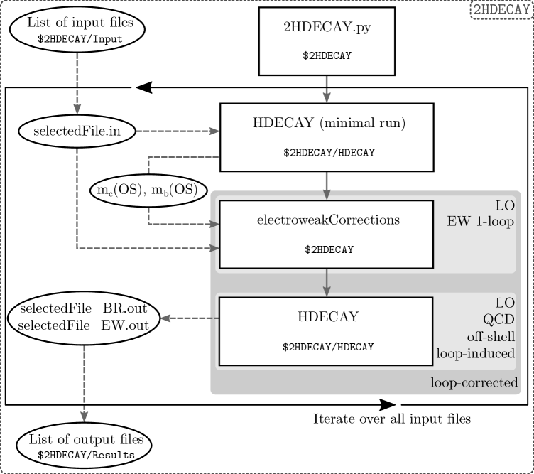
Figure 3: Flowchart of 2HDECAY. The main wrapper file 2HDECAY.py generates a list of input files, provided by the user in the subfolder $2HDECAY/Input, and iterates over the list. For each selected input file in the list, the wrapper calls HDECAY and the subprogram electroweakCorrections. The computed branching ratios including the EW and QCD corrections as described in the text are written to the output file with suffix ’_BR’, the calculated LO and NLO EW-corrected partial decay widths are given out in the output file with suffix ’_EW’. For further details, we refer to the text.

First, the wrapper file generates a list of all input files that the user provides in $2HDECAY/Input. The user can provide an arbitrary non-zero amount of input files with arbitrary filenames, as described in Sec. 3.5. For any input file in the list, the wrapper file first calls HDECAY in a so-called minimal run, technically by calling HDECAY in the subfolder $2HDECAY/HDECAY with an additional flag “1”:

⬇

run 1

With this flag, HDECAY reads the selected input file from the input file list and uses the input values only to convert the $\overline{\text{MS}}$ values of the $c$- and $b$-quark masses, as given in the input file, to the corresponding pole masses, but no other computations are performed at this step.

The wrapper file then calls the subprogram electroweakCorrections, which reads the selected input file as well as the OS values of the quark masses. With these input values, the full EW one-loop corrections are calculated for all decays that are kinematically allowed, as described in Sec. 2.3, and the value of $G_{F}^{\text{calc}}$ at the $Z$ mass is calculated, as described in Sec. 2.4. Subsequently, a temporary new input file is created, which consists of a copy of the selected input file with the calculated OS quark masses, the calculated value of $G_{F}^{\text{calc}}$ and all EW corrections being appended.

Lastly, the wrapper file calls HDECAY without the minimal flag. In this configuration, HDECAY reads the temporary input file and calculates the LO widths and QCD corrections to the decays. Moreover, the program calculates off-shell decay widths as well as the loop-induced decays to final-state pairs of gluons or photons and $Z\gamma$. Furthermore, the branching ratios are calculated by HDECAY. The results of these computations are consistently combined with the electroweak corrections, as described in Sec. 2.4. The results are saved in an output file in the $2HDECAY/Results subfolder.

The wrapper file repeats these steps for each file in the input file list until the end of the list is reached.

3.7 Usage

Before running the program, the user should check that all input files for which the computation shall be performed are stored in the subfolder $2HDECAY/Input. The input files have to be formatted exactly as described in Sec. 3.5 or otherwise the input values are not read in correctly and the program might crash with a segmentation error. The exemplary input file printed in App. A that is part of the 2HDECAY repository can be used as a template for generating other input files in order to avoid formatting problems.

The user should check the output subfolder $2HDECAY/Results for any output files of previous runs of 2HDECAY. These previously created output files are overwritten if in a new run input files with the same names as the already stored output files are used. Hence, the user is advised to create backups of the output files before starting a new run of 2HDECAY.

In order to run the program, open a terminal, navigate to the $2HDECAY folder and execute the following command:

⬇

python 2HDECAY.py

If 2HDECAY was installed correctly according to Sec. 3.4 and if the input files have the correct format, the program should now compute the EW and/or QCD corrections according to the flowchart shown in Fig. 3. Several intermediate results and information about the computation are printed in the terminal. As soon as the computation for all input files is done, 2HDECAY is terminated and the resulting output files can be found in the $2HDECAY/Results subfolder.

3.8 Output File Format

For each input file, two output files with the suffixes ’_QCD’ and ’_EW’ for the branching ratios and electroweak partial decay widths, respectively, are generated in an SLHA format, as described in Sec. 2.4. The SLHA output format [126, 127, 128] in its strict and original sense has only been designed for supersymmetric models. We have modified the format to account for the EW corrections that are implemented in 2HDECAY in the 2HDM. As a reference for the following description, exemplary output files are given in App. B. These modified SLHA output files are only generated if OMIT ELW2=0 is set in the input file, i.e. only if the electroweak corrections to the 2HDM decays are taken into account. In the following we describe the changes that we have applied.

The first block BLOCK DCINFO contains basic information about the program itself, while the subsequent three blocks SMINPUTS, 2HDMINPUTS and VCKMIN contain the input parameters used for the calculation that were already described in Sec. 3.5. As explained in Sec. 2.4, the value of $G_{F}$ printed in the output file is not necessarily the same as the one given in the input file if OMIT ELW2=0 is set, since in this case, $G_{F}$ is calculated from the input value $\alpha_{\text{em}}(m_{Z}^{2})$ instead, and this value is then given out. These four blocks are given out in both output files.

In the output file containing the branching ratios, indicated by the suffix ’_BR’, subsequently two blocks follow for each Higgs boson ($h,H,A$ and $H^{\pm}$). They are called DECAY QCD and DECAY QCD&EW. The block DECAY QCD contains the total decay width, the mixing angles $\alpha$, $\beta$, the $\overline{\mbox{MS}}$ parameter $m_{12}^{2}$, and the branching ratios of the decays of the respective Higgs boson, as implemented in HDECAY. These are in particular the LO (loop-induced for the $gg$, $\gamma\gamma$ and $Z\gamma$ final states) decay widths including the relevant and state-of-the art QCD corrections where applicable (cf. [79, 80] for further details). For decays into heavy quarks, massive vector bosons, neutral Higgs pairs as well as gauge and Higgs boson final states also off-shell decays are computed if necessary. We want to emphasize again that the partial and total decay widths differ from the ones of the original HDECAY version if OMIT ELW2=0 is set, as for consistency with the computed EW corrections in this case the HDECAY decay widths are rescaled by $G_{F}^{\text{calc}}/G_{F}$, as explained in Sec. 2.4. If OMIT ELW2=1 is set, no EW corrections are computed and the HDECAY decay widths are computed with $G_{F}$ as in the original HDECAY version.

The block DECAY QCD&EW contains the total decay width, the mixing angles $\alpha$, $\beta$, the $\overline{\mbox{MS}}$ parameter $m_{12}^{2}$, and the branching ratios of the respective Higgs boson including both the QCD corrections (provided by HDECAY) and the EW corrections (computed by 2HDECAY) to the LO decay widths. Note that the LO decay widths are also computed by 2HDECAY. As an additional cross-check, we internally compare the respective HDECAY LO decay width (rescaled by $G_{F}^{\text{calc}}/G_{F}$ and calculated with OS masses for this comparison) with the one computed by 2HDECAY. If they differ (which they should not), a warning is printed on the screen. As described in Sec. 2.4, we emphasize again that the EW corrections are calculated and included only for OS decay channels that are kinematically allowed and for non-loop-induced decays. Therefore, some of the branching ratios given out may be QCD-, but not EW-corrected. The total decay width given out in this block is the sum of all accordingly computed partial decay widths.

The last block at the end of the file with the branching ratios contains the QCD-corrected branching ratios of the top-quark calculated in the 2HDM. It is required for the computation of the Higgs decays into final states with an off-shell top.

In the output file with the EW corrected NLO decay widths, indicated by the suffix ’_EW’, the first four blocks described above are instead followed by the two blocks LO DECAY WIDTH and NLO DECAY WIDTH for each Higgs boson ($h,H,A$ and $H^{\pm}$). In these blocks, the partial decay widths at LO and including the one-loop EW corrections are given out, respectively, together with the mixing angles $\alpha$, $\beta$ and the $\overline{\mbox{MS}}$ parameter $m_{12}^{2}$. These values of the widths are particularly useful for studies of the relative size of the EW corrections and for studying the renormalization scheme dependence of the EW corrections. This allows for a rough estimate of the remaining theoretical error due to missing higher-order EW corrections. Since the EW corrections are calculated only for OS decays and additionally only for decays that are not loop-induced, these two blocks do not contain all final states written out in the blocks DECAY QCD and DECAY QCD&EW. Hence, depending on the input values that are chosen, it can happen that the two blocks DECAY QCD and DECAY QCD&EW contain decays that are not printed out in the blocks LO DECAY WIDTH and NLO DECAY WIDTH, since for the calculation of the branching ratios, off-shell and loop-induced decays are considered by HDECAY as well.

4 Summary

We have presented the program package 2HDECAY for the calculation of the Higgs boson decays in the 2HDM. The tool computes the NLO EW corrections to all 2HDM Higgs boson decays into OS final states that are not loop-induced. The user can choose among 17 different renormalization schemes that have been specified in the manual. They are based on different renormalization schemes for the mixing angles $\alpha$ and $\beta$, an $\overline{\text{MS}}$ condition for the soft-$\mathbb{Z}_{2}$-breaking scale $m_{12}^{2}$ and an OS scheme for all other counterterms and wave function renormalization constants of the 2HDM necessary for calculating the EW corrections. The EW corrections are combined with the state-of-the-art QCD corrections obtained from HDECAY. The EW&QCD-corrected total decay widths and branching ratios are given out in an SLHA-inspired output file format. Moreover, the tool provides separately an SLHA-inspired output for the LO and EW NLO partial decay widths to all OS and non-loop-induced decays. This separate output enables e.g. an efficient analysis of the size of the EW corrections in the 2HDM or the comparison with the relative EW corrections in the MSSM as a SUSY benchmark model. The implementation of several different renormalization schemes additionally allows for the investigation of the numerical effects of the different schemes and an estimate of the residual theoretical uncertainty due to missing higher-order EW corrections. For a consistent estimate of this error, an automatic parameter conversion routine is implemented, performing the automatic conversion of the input values of $\alpha$, $\beta$ and $m_{12}^{2}$ from a reference scheme to all other renormalization schemes that are implemented, as well as from the $\overline{\text{MS}}$ input renormalization scale $\mu_{R}$ to the renormalization scale $\mu_{\text{out}}$ at which the partial decay widths are evaluated. Being fast, our new tool enables efficient phenomenological studies of the 2HDM Higgs sector at high precision. The latter is necessary to reveal indirect new physics effects in the Higgs sector and to identify the true underlying model in case of the discovery of additional Higgs bosons. This brings us closer to our goal of understanding electroweak symmetry breaking and deciphering the physics puzzle in fundamental particle physics.

Acknowledgments

The authors thank David Lopez-Val and Jonas Müller for independently cross-checking some of the analytic results derived for this work. The authors express gratitude to David Lopez-Val for his endeavors on debugging the early alpha versions of 2HDECAY and to Stefan Liebler and Florian Staub for helpful discussions concerning the real corrections to the decays. The authors thank Ansgar Denner, Stefan Dittmaier and Jean-Nicolas Lang for helpful discussions and for providing the analytic results of their mixing angle counterterms to us for the implementation in 2HDECAY. MK and MM acknowledge financial support from the DFG project “Precision Calculations in the Higgs Sector - Paving the Way to the New Physics Landscape” (ID: MU 3138/1-1).

Appendix A Exemplary Input File

In the following, we present an exemplary input file 2hdecay.in as it is included in the subfolder $2HDECAY/Input in the 2HDECAY repository. The first integer in each line represents the line number and is not part of the actual input file, but printed here for convenience. The meaning of the input parameters is specified in Sec. 3.5. In comparison to the input file format of the unmodified HDECAY program[79, 80], the lines 6, 26, 28, 58, 59, 63 and 64 are new, but the rest of the input file format is unchanged. We want to emphasize again that the value GFCALC in the input file is overwritten by the program and thus not an input value that is provided by the user, but it is calculated by 2HDECAY internally. The sample 2HDM parameter point has been checked against all relevant theoretical and experimental constraints. In particular it features a SM-like Higgs boson with a mass of 125.09 GeV which is given by the lightest CP-even neutral Higgs boson $h$. For details on the applied constraints, we refer to Refs. [38, 129].

⬇

1SLHAIN = 1

2SLHAOUT = 1

3COUPVAR = 1

4HIGGS = 5

5OMIT ELW = 1

6OMIT ELW2= 0

7SM4 = 0

8FERMPHOB = 0

92HDM = 1

10MODEL = 1

11TGBET = 5.07403e+01

12MABEG = 4.67967e+02

13MAEND = 4.67967e+02

14NMA = 1

15********************* hMSSM (MODEL = 10) *********************************

16MHL = 125.D0

17**************************************************************************

18ALS(MZ) = 1.18000e-01

19MSBAR(2) = 9.50000e-02

20MCBAR(3) = 0.98600e+00

21MBBAR(MB)= 4.18000e+00

22MT = 1.73200e+02

23MTAU = 1.77682e+00

24MMUON = 1.056583715e-01

251/ALPHA = 1.37036e+02

26ALPHAMZ = 7.754222173973729e-03

27GF = 1.1663787e-05

28GFCALC = 0.000000000

29GAMW = 2.08500e+00

30GAMZ = 2.49520e+00

31MZ = 9.11876e+01

32MW = 8.0385e+01

33VTB = 9.9910e-01

34VTS = 4.040e-02

35VTD = 8.67e-03

36VCB = 4.12e-02

37VCS = 9.7344e-01

38VCD = 2.252e-01

39VUB = 3.51e-03

40VUS = 2.2534e-01

41VUD = 9.7427e-01

42********************* 4TH GENERATION *************************************

43 SCENARIO FOR ELW. CORRECTIONS TO H -> GG (EVERYTHING IN GEV):

44 GG_ELW = 1: MTP = 500 MBP = 450 MNUP = 375 MEP = 450

45 GG_ELW = 2: MBP = MNUP = MEP = 600 MTP = MBP+50*(1+LOG(M_H/115)/5)

46

47GG_ELW = 1

48MTP = 500.D0

49MBP = 450.D0

50MNUP = 375.D0

51MEP = 450.D0

52************************** 2 Higgs Doublet Model *************************

53 TYPE: 1 (I), 2 (II), 3 (lepton-specific), 4 (flipped)

54 PARAM: 1 (masses), 2 (lambda_i)

55

56PARAM = 1

57TYPE = 1

58RENSCHEM = 7

59REFSCHEM = 5

60********************

61TGBET2HDM= 4.23635D0

62M_12^2 = 28505.5D0

63INSCALE = 125.09D0

64OUTSCALE = MIN

65******************** PARAM=1:

66ALPHA_H = -0.189345D0

67MHL = 125.09D0

68MHH = 381.767D0

69MHA = 350.665D0

70MH+- = 414.114D0

71******************** PARAM=2:

72LAMBDA1 = 6.368674377530086700D0

73LAMBDA2 = 0.235570240072350970D0

74LAMBDA3 = 1.780416490847621700D0

75LAMBDA4 = -1.52623758540479430D0

76LAMBDA5 = 0.074592764717552856D0

77**************************************************************************

78SUSYSCALE= 2.22449e+03

79MU = -1.86701e+03

80M2 = -2.39071e+02

81MGLUINO = 7.32754e+02

82MSL1 = 1.49552e+03

83MER1 = 1.62210e+03

84MQL1 = 9.30379e+01

85MUR1 = 2.77029e+03

86MDR1 = 1.76481e+03

87MSL = 1.97714e+03

88MER = 9.29678e+02

89MSQ = 2.68124e+03

90MUR = 1.85939e+03

91MDR = 2.28235e+03

92AL = -4.62984e+03

93AU = 5.31164e+03

94AD = 2.54430e+03

95ON-SHELL = 0

96ON-SH-WZ = 0

97IPOLE = 0

98OFF-SUSY = 0

99INDIDEC = 0

100NF-GG = 5

101IGOLD = 0

102MPLANCK = 2.40000e+18

103MGOLD = 1.00000e-13

104******************* VARIATION OF HIGGS COUPLINGS *************************

105ELWK = 1

106CW = 1.D0

107CZ = 1.D0

108Ctau = 1.D0

109Cmu = 1.D0

110Ct = 1.D0

111Cb = 1.D0

112Cc = 1.D0

113Cs = 1.D0

114Cgaga = 0.D0

115Cgg = 0.D0

116CZga = 0.D0

117********************* 4TH GENERATION *************************************

118Ctp = 0.D0

119Cbp = 0.D0

120Cnup = 0.D0

121Cep = 0.D0

Appendix B Exemplary Output Files

In the following, we present exemplary output files 2hdecay_BR.out and 2hdecay_EW.out as they are generated from the sample input file 2hdecay.in and included in the subfolder
$2HDECAY/Results in the 2HDECAY repository. The suffixes “_BR” and “_EW” stand for the branching ratios and electroweak partial decay widths, respectively. The first integer in each line represents the line number and is not part of the actual output file, but printed here for convenience. The output file format is explained in detail in Sec. 3.8. The exemplary output file was generated for a specific choice of the renormalization scheme, i.e. we have set RENSCHEM = 7 in line 58 of the input file, cf. App. A. For RENSCHEM = 0, the output file becomes considerably longer, since the electroweak corrections are calculated for all 17 implemented renormalization schemes. We chose REFSCHEM = 5 and INSCALE = 125.09D0. This means that the input values for $\alpha$ and $\beta$ are understood to be given in the renormalization scheme 5 and the scale at which $\alpha$, $\beta$ and the $\overline{\mbox{MS}}$ parameter $m_{12}^{2}$ are defined is equal to 125.09 GeV.

B.1 Exemplary Output File for the Branching Ratios

The exemplary output file 2hdecay_BR.out contains the branching ratios without and with the electroweak corrections. The content of the file is presented in the following.

⬇

1#

2BLOCK DCINFO # Decay Program information

3 1 2HDECAY # decay calculator

4 2 1.1.0 # version number

5#

6BLOCK SMINPUTS # Standard Model inputs

7 2 1.19596488E-05 # G_F [GeV^-2]

8 3 1.18000000E-01 # alpha_S(M_Z)^MSbar

9 4 9.11876000E+01 # M_Z on-shell mass

10 5 4.18000000E+00 # mb(mb)^MSbar

11 6 1.73200000E+02 # mt pole mass

12 7 1.77682000E+00 # mtau pole mass

13 8 4.84141297E+00 # mb pole mass

14 9 1.43141297E+00 # mc pole mass

15 10 1.05658372E-01 # muon mass

16 11 8.03850000E+01 # M_W on-shell mass

17 12 2.08500000E+00 # W boson total width

18 13 2.49520000E+00 # Z boson total width

19#

20BLOCK 2HDMINPUTS # 2HDM inputs of reference scheme

21 1 1 # 2HDM parametrization

22 2 1 # 2HDM type

23 3 4.23635000E+00 # tan(beta)

24 4 2.85055000E+04 # M_12^2

25 5 -1.89345000E-01 # alpha

26 6 1.25090000E+02 # M_h

27 7 3.81767000E+02 # M_H

28 8 3.50665000E+02 # M_A

29 9 4.14114000E+02 # M_CH

30 10 6.53022117E+00 # LAMBDA1 calc. from masses/alpha

31 11 2.41545678E-01 # LAMBDA2 calc. from masses/alpha

32 12 1.82557826E+00 # LAMBDA3 calc. from masses/alpha

33 13 -1.56495189E+00 # LAMBDA4 calc. from masses/alpha

34 14 7.64848730E-02 # LAMBDA5 calc. from masses/alpha

35 15 7 # renormalization scheme EW corrs

36 16 5 # reference ren. scheme EW corrs

37 17 125.09D0 # ren. scale of MSbar parameters

38 18 MIN # ren. scale at which decay is evaluated

39#

40BLOCK VCKMIN # CKM mixing

41 1 9.99100000E-01 # V_tb

42 2 4.04000000E-02 # V_ts

43 3 8.67000000E-03 # V_td

44 4 4.12000000E-02 # V_cb

45 5 9.73440000E-01 # V_cs

46 6 2.25200000E-01 # V_cd

47 7 3.51000000E-03 # V_ub

48 8 2.25340000E-01 # V_us

49 9 9.74270000E-01 # V_ud

50#

51# PDG Width QCD Only

52DECAY QCD 25 4.22730978E-03 # h decays with QCD corrections only

53 7 # Renormalization Scheme Number

54 -0.18809815E+00 # Corresponding mixing angle alpha

55 0.43048897E+01 # Corresponding tan(beta)

56 0.28505500E+05 # Corresponding m_12^2

57# BR NDA ID1 ID2

58 5.93838905E-01 2 5 -5 # BR(h -> b bb )

59 6.38675293E-02 2 -15 15 # BR(h -> tau+ tau- )

60 2.26112814E-04 2 -13 13 # BR(h -> mu+ mu- )

61 2.24253909E-04 2 3 -3 # BR(h -> s sb )

62 2.90727883E-02 2 4 -4 # BR(h -> c cb )

63 7.76755623E-02 2 21 21 # BR(h -> g g )

64 2.19865876E-03 2 22 22 # BR(h -> gam gam )

65 1.54187689E-03 2 22 23 # BR(h -> Z gam )

66 2.05662673E-01 2 24 -24 # BR(h -> W+ W- )

67 2.56916399E-02 2 23 23 # BR(h -> Z Z )

68#

69# PDG Width QCD and EW

70DECAY QCD&EW 25 4.10575180E-03 # h decays with QCD and EW corrections

71 7 # Renormalization Scheme Number

72 -0.18809815E+00 # Corresponding mixing angle alpha

73 0.43048897E+01 # Corresponding tan(beta)

74 0.28505500E+05 # Corresponding m_12^2

75# BR NDA ID1 ID2

76 5.85412930E-01 2 5 -5 # BR(h -> b bb )

77 6.30251890E-02 2 -15 15 # BR(h -> tau+ tau- )

78 2.18258112E-04 2 -13 13 # BR(h -> mu+ mu- )

79 2.25768642E-04 2 3 -3 # BR(h -> s sb )

80 2.90873264E-02 2 4 -4 # BR(h -> c cb )

81 7.99752836E-02 2 21 21 # BR(h -> g g )

82 2.26375391E-03 2 22 22 # BR(h -> gam gam )

83 1.58752686E-03 2 22 23 # BR(h -> Z gam )

84 2.11751677E-01 2 24 -24 # BR(h -> W+ W- )

85 2.64522859E-02 2 23 23 # BR(h -> Z Z )

86#

87# PDG Width QCD Only

88DECAY QCD 35 1.82054627E-01 # H decays with QCD corrections only

89 7 # Renormalization Scheme Number

90 -0.18809815E+00 # Corresponding mixing angle alpha

91 0.43048897E+01 # Corresponding tan(beta)

92 0.28286295E+05 # Corresponding m_12^2

93# BR NDA ID1 ID2

94 1.23718494E-03 2 5 -5 # BR(H -> b bb )

95 1.64167073E-04 2 -15 15 # BR(H -> tau+ tau- )

96 5.80581591E-07 2 -13 13 # BR(H -> mu+ mu- )

97 4.66487784E-07 2 3 -3 # BR(H -> s sb )

98 6.05366336E-05 2 4 -4 # BR(H -> c cb )

99 5.39857087E-01 2 6 -6 # BR(H -> t tb )

100 4.22983124E-03 2 21 21 # BR(H -> g g )

101 1.81583473E-05 2 22 22 # BR(H -> gam gam )

102 1.06915278E-05 2 22 23 # BR(H -> Z gam )

103 1.27161194E-01 2 24 -24 # BR(H -> W+ W- )

104 5.90077292E-02 2 23 23 # BR(H -> Z Z )

105 1.19027442E-10 2 36 36 # BR(H -> A A )

106 2.68081410E-01 2 25 25 # BR(H -> h h )

107 1.70962359E-04 2 23 36 # BR(H -> Z A )

108#

109# PDG Width QCD and EW

110DECAY QCD&EW 35 2.02874707E-01 # H decays with QCD and EW corrections

111 7 # Renormalization Scheme Number

112 -0.18809815E+00 # Corresponding mixing angle alpha

113 0.43048897E+01 # Corresponding tan(beta)

114 0.28286295E+05 # Corresponding m_12^2

115# BR NDA ID1 ID2

116 1.05832016E-03 2 5 -5 # BR(H -> b bb )

117 1.33470074E-04 2 -15 15 # BR(H -> tau+ tau- )

118 4.61132083E-07 2 -13 13 # BR(H -> mu+ mu- )

119 3.90544832E-07 2 3 -3 # BR(H -> s sb )

120 5.01923622E-05 2 4 -4 # BR(H -> c cb )

121 4.75365783E-01 2 6 -6 # BR(H -> t tb )

122 3.79574350E-03 2 21 21 # BR(H -> g g )

123 1.62948412E-05 2 22 22 # BR(H -> gam gam )

124 9.59430645E-06 2 22 23 # BR(H -> Z gam )

125 1.19103021E-01 2 24 -24 # BR(H -> W+ W- )

126 6.65098085E-02 2 23 23 # BR(H -> Z Z )

127 1.06812214E-10 2 36 36 # BR(H -> A A )

128 3.33803504E-01 2 25 25 # BR(H -> h h )

129 1.53417294E-04 2 23 36 # BR(H -> Z A )

130#

131# PDG Width QCD Only

132DECAY QCD 36 4.12723113E-01 # A decays with QCD corrections only

133 7 # Renormalization Scheme Number

134 -0.18809815E+00 # Corresponding mixing angle alpha

135 0.43048897E+01 # Corresponding tan(beta)

136 0.28302990E+05 # Corresponding m_12^2

137# BR NDA ID1 ID2

138 7.27392605E-04 2 5 -5 # BR(A -> b bb )

139 9.74019639E-05 2 -15 15 # BR(A -> tau+ tau- )

140 3.44437869E-07 2 -13 13 # BR(A -> mu+ mu- )

141 2.60982854E-07 2 3 -3 # BR(A -> s sb )

142 3.67755809E-05 2 4 -4 # BR(A -> c cb )

143 9.62219843E-01 2 6 -6 # BR(A -> t tb )

144 9.63661208E-03 2 21 21 # BR(A -> g g )

145 3.97340998E-05 2 22 22 # BR(A -> gam gam )

146 6.75641349E-06 2 22 23 # BR(A -> Z gam )

147 2.72348787E-02 2 23 25 # BR(A -> Z h )

148#

149# PDG Width QCD and EW

150DECAY QCD&EW 36 4.10006463E-01 # A decays with QCD and EW corrections

151 7 # Renormalization Scheme Number

152 -0.18809815E+00 # Corresponding mixing angle alpha

153 0.43048897E+01 # Corresponding tan(beta)

154 0.28302990E+05 # Corresponding m_12^2

155# BR NDA ID1 ID2

156 6.84138168E-04 2 5 -5 # BR(A -> b bb )

157 8.64209164E-05 2 -15 15 # BR(A -> tau+ tau- )

158 2.98361191E-07 2 -13 13 # BR(A -> mu+ mu- )

159 2.38527876E-07 2 3 -3 # BR(A -> s sb )

160 3.32826226E-05 2 4 -4 # BR(A -> c cb )

161 9.70984653E-01 2 6 -6 # BR(A -> t tb )

162 9.70046304E-03 2 21 21 # BR(A -> g g )

163 3.99973728E-05 2 22 22 # BR(A -> gam gam )

164 6.80118062E-06 2 22 23 # BR(A -> Z gam )

165 1.84637072E-02 2 23 25 # BR(A -> Z h )

166#

167# PDG Width QCD Only

168DECAY QCD 37 9.52122446E-01 # H+ decays with QCD corrections only

169 7 # Renormalization Scheme Number

170 -0.18809815E+00 # Corresponding mixing angle alpha

171 0.43048897E+01 # Corresponding tan(beta)

172 0.28270317E+05 # Corresponding m_12^2

173# BR NDA ID1 ID2

174 6.38478540E-07 2 4 -5 # BR(H+ -> c bb )

175 4.98617485E-05 2 -15 16 # BR(H+ -> tau+ nu_t au )

176 1.76321144E-07 2 -13 14 # BR(H+ -> mu+ nu_m u )

177 4.41813442E-09 2 2 -5 # BR(H+ -> u bb )

178 6.73510166E-09 2 2 -3 # BR(H+ -> u sb )

179 8.84349820E-07 2 4 -1 # BR(H+ -> c db )

180 1.66493576E-05 2 4 -3 # BR(H+ -> c sb )

181 9.70305009E-01 2 6 -5 # BR(H+ -> t bb )

182 1.58487563E-03 2 6 -3 # BR(H+ -> t sb )

183 7.29902662E-05 2 6 -1 # BR(H+ -> t db )

184 2.60001008E-02 2 24 25 # BR(H+ -> W+ h )

185 5.03002930E-05 2 24 35 # BR(H+ -> W+ H )

186 1.91850311E-03 2 24 36 # BR(H+ -> W+ A )

187#

188# PDG Width QCD and EW

189DECAY QCD&EW 37 9.15926373E-01 # H+ decays with QCD and EW corrections

190 7 # Renormalization Scheme Number

191 -0.18809815E+00 # Corresponding mixing angle alpha

192 0.43048897E+01 # Corresponding tan(beta)

193 0.28270317E+05 # Corresponding m_12^2

194# BR NDA ID1 ID2

195 5.95091084E-07 2 4 -5 # BR(H+ -> c bb )

196 4.71994255E-05 2 -15 16 # BR(H+ -> tau+ nu_tau )

197 1.63076322E-07 2 -13 14 # BR(H+ -> mu+ nu_mu )

198 3.64995618E-09 2 2 -5 # BR(H+ -> u bb )

199 6.55853493E-09 2 2 -3 # BR(H+ -> u sb )

200 8.55031171E-07 2 4 -1 # BR(H+ -> c db )

201 1.60986318E-05 2 4 -3 # BR(H+ -> c sb )

202 9.66117646E-01 2 6 -5 # BR(H+ -> t bb )

203 1.58023685E-03 2 6 -3 # BR(H+ -> t sb )

204 7.31159911E-05 2 6 -1 # BR(H+ -> t db )

205 3.01174725E-02 2 24 25 # BR(H+ -> W+ h )

206 5.22880871E-05 2 24 35 # BR(H+ -> W+ H )

207 1.99431955E-03 2 24 36 # BR(H+ -> W+ A )

208#

209# PDG Width

210DECAY 6 1.36958730E+00 # top decays

211# BR NDA ID1 ID2

212 1.00000000E+00 2 5 24 # BR(t -> b W+ )

In the following, we make some comments on the output files that partly pick up hints and caveats made in the main text of the manual. As can be inferred from the output, we give for the decays of each Higgs boson the values of $\alpha$, $\beta$ and $m_{12}^{2}$. These values change from the input values and for each Higgs boson as we have to perform the parameter conversion from the input reference scheme 5 to the renormalization scheme 7 and because we use for the loop corrected widths the renormalization scale given by the mass of the decaying Higgs boson, since we set OUTSCALE = MIN while the input values for these parameters are understood to be given at the mass of the SM-like Higgs boson. Furthermore notice that indeed the branching ratios of the lightest CP-even Higgs boson $h$ are SM-like. All branching ratios presented in the blocks DECAY QCD can be compared to the ones generated by the program code HDECAY version 6.52. The user will notice that the partial widths related to the branching ratios generated by 2HDECAY and HDECAY, respectively, differ due to the rescaling factor $G_{F}^{\text{calc}}/G_{F}=1.026327$, which is applied in 2HDECAY for the consistent combination of the EW-corrected decay widths with the decay widths generated by HDECAY. Be aware that the rescaling factor appears in the loop induced decay into $Z\gamma$ and in the off-shell decays non-linearly. This is why also the branching ratios given here differ from the ones generated by HDECAY6.52. The comparison furthermore shows an additional difference between the decay widths for the heavy CP-even Higgs boson $H$ into massive vector bosons, $\Gamma(H\to VV)$ ($V=W,Z$), of around 2-3%. The reason is that HDECAY throughout computes these decay widths using the double off-shell formula while 2HDECAY uses the on-shell formula for Higgs boson masses above the threshold. Let us also note some phenomenological features of the chosen parameter point. The $H$ boson with a mass of 382 GeV is heavy enough to decay on-shell into $WW$ and $ZZ$, and also into the 2-Higgs boson final state $hh$. It decays off-shell into $AA$ and the gauge plus Higgs boson final state $ZA$ with branching ratios of ${\cal O}(10^{-10})$ and ${\cal O}(10^{-4})$, respectively. The pseudoscalar with a mass of 351 GeV decays on-shell into the gauge plus Higgs boson final state $Zh$ with a branching ratio at the per cent level. The charged Higgs boson has a mass of 414 GeV allowing it to decay on-shell in the gauge plus Higgs boson final state $W^{+}h$ with a branching ratio at the per cent level. It decays off-shell into the final states $W^{+}H$ and $W^{+}A$ with branching ratios of ${\cal O}(10^{-5})$ and ${\cal O}(10^{-3})$, respectively.

B.2 Exemplary Output File for the Electroweak Partial Decay Widths

The exemplary output file 2hdecay_EW.out contains the LO and electroweak NLO partial decay widths. The content of the file is presented in the following.

⬇

1#

2BLOCK DCINFO # Decay Program information

3 1 2HDECAY # decay calculator

4 2 1.1.0 # version number

5#

6BLOCK SMINPUTS # Standard Model inputs

7 2 1.19596488E-05 # G_F [GeV^-2]

8 3 1.18000000E-01 # alpha_S(M_Z)^MSbar

9 4 9.11876000E+01 # M_Z on-shell mass

10 5 4.18000000E+00 # mb(mb)^MSbar

11 6 1.73200000E+02 # mt pole mass

12 7 1.77682000E+00 # mtau pole mass

13 8 4.84141297E+00 # mb pole mass

14 9 1.43141297E+00 # mc pole mass

15 10 1.05658372E-01 # muon mass

16 11 8.03850000E+01 # M_W on-shell mass

17 12 2.08500000E+00 # W boson total width

18 13 2.49520000E+00 # Z boson total width

19#

20BLOCK 2HDMINPUTS # 2HDM inputs of reference scheme

21 1 1 # 2HDM parametrization

22 2 1 # 2HDM type

23 3 4.23635000E+00 # tan(beta)

24 4 2.85055000E+04 # M_12^2

25 5 -1.89345000E-01 # alpha

26 6 1.25090000E+02 # M_h

27 7 3.81767000E+02 # M_H

28 8 3.50665000E+02 # M_A

29 9 4.14114000E+02 # M_CH

30 10 6.53022117E+00 # LAMBDA1 calc. from masses/alpha

31 11 2.41545678E-01 # LAMBDA2 calc. from masses/alpha

32 12 1.82557826E+00 # LAMBDA3 calc. from masses/alpha

33 13 -1.56495189E+00 # LAMBDA4 calc. from masses/alpha

34 14 7.64848730E-02 # LAMBDA5 calc. from masses/alpha

35 15 7 # renormalization scheme EW corrs

36 16 5 # reference ren. scheme EW corrs

37 17 125.09D0 # input scale

38 18 MIN # ren. scale at which decay is evaluated

39#

40BLOCK VCKMIN # CKM mixing

41 1 9.99100000E-01 # V_tb

42 2 4.04000000E-02 # V_ts

43 3 8.67000000E-03 # V_td

44 4 4.12000000E-02 # V_cb

45 5 9.73440000E-01 # V_cs

46 6 2.25200000E-01 # V_cd

47 7 3.51000000E-03 # V_ub

48 8 2.25340000E-01 # V_us

49 9 9.74270000E-01 # V_ud

50#

51# PDG

52LO DECAY WIDTH 25 # h non-zero LO EW decay widths of on-shell and non-loop induced decays

53 7 # Renormalization Scheme Number

54 -0.18809815E+00 # Corresponding mixing angle alpha

55 0.43048897E+01 # Corresponding tan(beta)

56 0.28505500E+05 # Corresponding m_12^2

57# WIDTH NDA ID1 ID2

58 5.96669359E-03 2 5 -5 # GAM(h -> b bb )

59 2.69987831E-04 2 -15 15 # GAM(h -> tau+ tau- )

60 9.55848909E-07 2 -13 13 # GAM(h -> mu+ mu- )

61 2.31819649E-06 2 3 -3 # GAM(h -> s sb )

62 5.25887869E-04 2 4 -4 # GAM(h -> c cb )

63#

64# PDG

65NLO DECAY WIDTH 25 # h non-zero NLO EW decay widths of on-shell and non-loop induced decays

66 7 # Renormalization Scheme Number

67 -0.18809815E+00 # Corresponding mixing angle alpha

68 0.43048897E+01 # Corresponding tan(beta)

69 0.28505500E+05 # Corresponding m_12^2

70# WIDTH NDA ID1 ID2

71 5.71289204E-03 2 5 -5 # GAM(h -> b bb )

72 2.58765783E-04 2 -15 15 # GAM(h -> tau+ tau- )

73 8.96113636E-07 2 -13 13 # GAM(h -> mu+ mu- )

74 2.26674392E-06 2 3 -3 # GAM(h -> s sb )

75 5.11021167E-04 2 4 -4 # GAM(h -> c cb )

76#

77# PDG

78LO DECAY WIDTH 35 # H non-zero LO EW decay widths of on-shell and non-loop induced decays

79 7 # Renormalization Scheme Number

80 -0.18809815E+00 # Corresponding mixing angle alpha

81 0.43048897E+01 # Corresponding tan(beta)

82 0.28286295E+05 # Corresponding m_12^2

83# WIDTH NDA ID1 ID2

84 6.65125616E-04 2 5 -5 # GAM(H -> b bb )

85 2.98873753E-05 2 -15 15 # GAM(H -> tau+ tau- )

86 1.05697565E-07 2 -13 13 # GAM(H -> mu+ mu- )

87 2.56345478E-07 2 3 -3 # GAM(H -> s sb )

88 5.81931534E-05 2 4 -4 # GAM(H -> c cb )

89 6.32882453E-02 2 6 -6 # GAM(H -> t tb )

90 2.31502837E-02 2 24 -24 # GAM(H -> W+ W- )

91 1.07426301E-02 2 23 23 # GAM(H -> Z Z )

92 4.88054612E-02 2 25 25 # GAM(H -> h h )

93#

94# PDG

95NLO DECAY WIDTH 35 # H non-zero NLO EW decay widths of on-shell and non-loop induced decays

96 7 # Renormalization Scheme Number

97 -0.18809815E+00 # Corresponding mixing angle alpha

98 0.43048897E+01 # Corresponding tan(beta)

99 0.28286295E+05 # Corresponding m_12^2

100# WIDTH NDA ID1 ID2

101 6.34033642E-04 2 5 -5 # GAM(H -> b bb )

102 2.70777021E-05 2 -15 15 # GAM(H -> tau+ tau- )

103 9.35520362E-08 2 -13 13 # GAM(H -> mu+ mu- )

104 2.39156652E-07 2 3 -3 # GAM(H -> s sb )

105 5.37672029E-05 2 4 -4 # GAM(H -> c cb )

106 6.21009650E-02 2 6 -6 # GAM(H -> t tb )

107 2.41629904E-02 2 24 -24 # GAM(H -> W+ W- )

108 1.34931579E-02 2 23 23 # GAM(H -> Z Z )

109 6.77202880E-02 2 25 25 # GAM(H -> h h )

110#

111# PDG

112LO DECAY WIDTH 36 # A non-zero LO decay widths of on-shell and non-loop induced decays

113 7 # Renormalization Scheme Number

114 -0.18809815E+00 # Corresponding mixing angle alpha

115 0.43048897E+01 # Corresponding tan(beta)

116 0.28302990E+05 # Corresponding m_12^2

117# WIDTH NDA ID1 ID2

118 8.95079946E-04 2 5 -5 # GAM(A -> b bb )

119 4.02000418E-05 2 -15 15 # GAM(A -> tau+ tau- )

120 1.42157470E-07 2 -13 13 # GAM(A -> mu+ mu- )

121 3.44770691E-07 2 3 -3 # GAM(A -> s sb )

122 7.82705947E-05 2 4 -4 # GAM(A -> c cb )

123 1.78189744E-01 2 6 -6 # GAM(A -> t tb )

124 1.12404639E-02 2 23 25 # GAM(A -> Z h )

125#

126# PDG

127NLO DECAY WIDTH 36 # A non-zero NLO EW decay widths of on-shell and non-loop induced decays

128 7 # Renormalization Scheme Number

129 -0.18809815E+00 # Corresponding mixing angle alpha

130 0.43048897E+01 # Corresponding tan(beta)

131 0.28302990E+05 # Corresponding m_12^2

132# WIDTH NDA ID1 ID2

133 8.36312673E-04 2 5 -5 # GAM(A -> b bb )

134 3.54331343E-05 2 -15 15 # GAM(A -> tau+ tau- )

135 1.22330017E-07 2 -13 13 # GAM(A -> mu+ mu- )

136 3.13032490E-07 2 3 -3 # GAM(A -> s sb )

137 7.03701609E-05 2 4 -4 # GAM(A -> c cb )

138 1.78629290E-01 2 6 -6 # GAM(A -> t tb )

139 7.57023930E-03 2 23 25 # GAM(A -> Z h )

140#

141# PDG

142LO DECAY WIDTH 37 # H+ non-zero LO decay widths of on-shell and non-loop induced decays

143 7 # Renormalization Scheme Number

144 -0.18809815E+00 # Corresponding mixing angle alpha

145 0.43048897E+01 # Corresponding tan(beta)

146 0.28270317E+05 # Corresponding m_12^2

147# WIDTH NDA ID1 ID2

148 1.95134769E-06 2 4 -5 # GAM(H+ -> c bb )

149 4.74744900E-05 2 -15 16 # GAM(H+ -> tau+ nu_tau)

150 1.67879319E-07 2 -13 14 # GAM(H+ -> mu+ nu_mu)

151 1.30241820E-08 2 2 -5 # GAM(H+ -> u bb )

152 2.06744724E-08 2 2 -3 # GAM(H+ -> u sb )

153 4.68777754E-06 2 4 -1 # GAM(H+ -> c db )

154 8.79746167E-05 2 4 -3 # GAM(H+ -> c sb )

155 9.20580564E-01 2 6 -5 # GAM(H+ -> t bb )

156 1.50367679E-03 2 6 -3 # GAM(H+ -> t sb )

157 6.92515961E-05 2 6 -1 # GAM(H+ -> t db )

158 2.47552795E-02 2 24 25 # GAM(H+ -> W+ h )

159#

160# PDG

161NLO DECAY WIDTH 37 # H+ non-zero NLO EW decay widths of on-shell and non-loop induced decays

162 7 # Renormalization Scheme Number

163 -0.18809815E+00 # Corresponding mixing angle alpha

164 0.43048897E+01 # Corresponding tan(beta)

165 0.28270317E+05 # Corresponding m_12^2

166# WIDTH NDA ID1 ID2

167 1.74960317E-06 2 4 -5 # GAM(H+ -> c bb )

168 4.32311986E-05 2 -15 16 # GAM(H+ -> tau+ nu_tau )

169 1.49365904E-07 2 -13 14 # GAM(H+ -> mu+ nu_mu )

170 1.03506338E-08 2 2 -5 # GAM(H+ -> u bb )

171 1.93671125E-08 2 2 -3 # GAM(H+ -> u sb )

172 4.36006145E-06 2 4 -1 # GAM(H+ -> c db )

173 8.18307685E-05 2 4 -3 # GAM(H+ -> c sb )

174 8.81761847E-01 2 6 -5 # GAM(H+ -> t bb )

175 1.44227891E-03 2 6 -3 # GAM(H+ -> t sb )

176 6.67336642E-05 2 6 -1 # GAM(H+ -> t db )

177 2.75853874E-02 2 24 25 # GAM(H+ -> W+ h )

The inspection of the output file shows that the EW corrections reduce the $h$ decay widths, and the relative NLO EW corrections, $\Delta^{\text{EW}}=(\Gamma^{\text{EW}}-\Gamma^{\text{LO}})/\Gamma^{\text{LO}}$, range between -6.3 and -2.2% for the decays $\Gamma(h\to\mu^{+}\mu^{-})$ and $\Gamma(h\to s\bar{s})$, respectively. Regarding $H$, the corrections can both enhance and reduce the decay widths. The relative corrections range between -11.5 and 27.7% for the decays $\Gamma(H\to\mu^{+}\mu^{-})$ and $\Gamma(H\to hh)$, respectively. The relative corrections to the $A$ decay widths vary between -31.2 and 0.3% for the decays $\Gamma(A\to Zh)$ and $\Gamma(A\to t\bar{t})$, respectively. And those for the $H^{\pm}$ decays between -20.6 and 11.1% for the decays $\Gamma(H^{+}\to u\bar{b})$ and $\Gamma(H^{+}\to W^{+}h)$, respectively. The EW corrections (for the renormalization scheme number 7) of the chosen parameter point can hence be sizeable. Finally, note also that LO and NLO EW-corrected decay widths are given out for on-shell and non-loop induced decays only.

References

- [1] ATLAS, G. Aad et al., Phys. Lett. B716, 1 (2012), arXiv:1207.7214.
- [2] CMS, S. Chatrchyan et al., Phys. Lett. B716, 30 (2012), arXiv:1207.7235.
- [3] ATLAS, CMS, G. Aad et al., Phys. Rev. Lett. 114, 191803 (2015), arXiv:1503.07589.
- [4] LHC Higgs Cross Section Working Group, D. de Florian et al., (2016), arXiv:1610.07922.
- [5] Yu. A. Golfand and E. P. Likhtman, JETP Lett. 13, 323 (1971), [Pisma Zh. Eksp. Teor. Fiz. 13, 452 (1971)].
- [6] D. Volkov and V. Akulov, Phys. Lett. B46, 109 (1973).
- [7] J. Wess and B. Zumino, Nucl. Phys. B70, 39 (1974).
- [8] P. Fayet, Nucl. Phys. B90, 104 (1975).
- [9] P. Fayet and S. Ferrara, Phys. Rept. 32, 249 (1977).
- [10] P. Fayet, Phys. Lett. 64B, 159 (1976).
- [11] P. Fayet, Phys. Lett. 69B, 489 (1977).
- [12] H. P. Nilles, Phys. Rept. 110, 1 (1984).
- [13] H. E. Haber and G. L. Kane, Phys. Rept. 117, 75 (1985).
- [14] M. Sohnius, Phys. Rept. 128, 39 (1985).
- [15] J. Gunion and H. E. Haber, Nucl. Phys. B272, 1 (1986).
- [16] J. Gunion and H. E. Haber, Nucl. Phys. B278, 449 (1986).
- [17] J. F. Gunion, H. E. Haber, G. L. Kane, and S. Dawson, Front. Phys. 80, 1 (2000).
- [18] S. P. Martin, Adv. Ser. Direct. High Energy Phys. 21, 1 (2010), hep-ph/9709356.
- [19] S. Dawson, p. 261 (1997), hep-ph/9712464.
- [20] A. Djouadi, Phys. Rept. 459, 1 (2008), hep-ph/0503173.
- [21] T. D. Lee, Phys. Rev. D8, 1226 (1973).
- [22] G. C. Branco et al., Phys. Rept. 516, 1 (2012), arXiv:1106.0034.
- [23] L. D. McLerran, M. E. Shaposhnikov, N. Turok, and M. B. Voloshin, Phys. Lett. B256, 451 (1991).
- [24] N. Turok and J. Zadrozny, Nucl. Phys. B358, 471 (1991).
- [25] A. G. Cohen, D. B. Kaplan, and A. E. Nelson, Phys. Lett. B263, 86 (1991).
- [26] N. Turok and J. Zadrozny, Nucl. Phys. B369, 729 (1992).
- [27] K. Funakubo, A. Kakuto, and K. Takenaga, Prog. Theor. Phys. 91, 341 (1994), hep-ph/9310267.
- [28] A. T. Davies, C. D. Froggatt, G. Jenkins, and R. G. Moorhouse, Phys. Lett. B336, 464 (1994).
- [29] J. M. Cline, K. Kainulainen, and A. P. Vischer, Phys. Rev. D54, 2451 (1996), hep-ph/9506284.
- [30] J. M. Cline and P.-A. Lemieux, Phys. Rev. D55, 3873 (1997), hep-ph/9609240.
- [31] L. Fromme, S. J. Huber, and M. Seniuch, JHEP 11, 038 (2006), hep-ph/0605242.
- [32] J. M. Cline, K. Kainulainen, and M. Trott, JHEP 11, 089 (2011), arXiv:1107.3559.
- [33] G. C. Dorsch, S. J. Huber, and J. M. No, JHEP 10, 029 (2013), arXiv:1305.6610.
- [34] K. Fuyuto and E. Senaha, Phys. Lett. B747, 152 (2015), arXiv:1504.04291.
- [35] G. C. Dorsch, S. J. Huber, K. Mimasu, and J. M. No, Phys. Rev. Lett. 113, 211802 (2014), arXiv:1405.5537.
- [36] G. C. Dorsch, S. J. Huber, K. Mimasu, and J. M. No, Phys. Rev. D93, 115033 (2016), arXiv:1601.04545.
- [37] G. C. Dorsch, S. J. Huber, T. Konstandin, and J. M. No, JCAP 1705, 052 (2017), arXiv:1611.05874.
- [38] P. Basler, M. Krause, M. Muhlleitner, J. Wittbrodt, and A. Wlotzka, JHEP 02, 121 (2017), arXiv:1612.04086.
- [39] G. C. Dorsch, S. J. Huber, K. Mimasu, and J. M. No, JHEP 12, 086 (2017), arXiv:1705.09186.
- [40] P. Basler, M. Muhlleitner, and J. Wittbrodt, JHEP 03, 061 (2018), arXiv:1711.04097.
- [41] P. Basler and M. Muhlleitner, (2018), arXiv:1803.02846.
- [42] N. G. Deshpande and E. Ma, Phys. Rev. D18, 2574 (1978).
- [43] R. Barbieri, L. J. Hall, and V. S. Rychkov, Phys. Rev. D74, 015007 (2006), hep-ph/0603188.
- [44] L. Lopez Honorez, E. Nezri, J. F. Oliver, and M. H. G. Tytgat, JCAP 0702, 028 (2007), hep-ph/0612275.
- [45] E. M. Dolle and S. Su, Phys. Rev. D80, 055012 (2009), arXiv:0906.1609.
- [46] L. Lopez Honorez and C. E. Yaguna, JHEP 09, 046 (2010), arXiv:1003.3125.
- [47] M. Gustafsson, S. Rydbeck, L. Lopez-Honorez, and E. Lundstrom, Phys. Rev. D86, 075019 (2012), arXiv:1206.6316.
- [48] B. Swiezewska, Phys. Rev. D88, 055027 (2013), arXiv:1209.5725, [Erratum: Phys. Rev. D88, no.11, 119903 (2013)].
- [49] B. Swiezewska and M. Krawczyk, Phys. Rev. D88, 035019 (2013), arXiv:1212.4100.
- [50] A. Arhrib, Y.-L. S. Tsai, Q. Yuan, and T.-C. Yuan, JCAP 1406, 030 (2014), arXiv:1310.0358.
- [51] M. Klasen, C. E. Yaguna, and J. D. Ruiz-Alvarez, Phys. Rev. D87, 075025 (2013), arXiv:1302.1657.
- [52] T. Abe, R. Kitano, and R. Sato, Phys. Rev. D91, 095004 (2015), arXiv:1411.1335, [Erratum: Phys. Rev. D96, no.1, 019902 (2017)].
- [53] M. Krawczyk, D. Sokolowska, P. Swaczyna, and B. Swiezewska, JHEP 09, 055 (2013), arXiv:1305.6266.
- [54] A. Goudelis, B. Herrmann, and O. Stål, JHEP 09, 106 (2013), arXiv:1303.3010.
- [55] N. Chakrabarty, D. K. Ghosh, B. Mukhopadhyaya, and I. Saha, Phys. Rev. D92, 015002 (2015), arXiv:1501.03700.
- [56] A. Ilnicka, M. Krawczyk, and T. Robens, Phys. Rev. D93, 055026 (2016), arXiv:1508.01671.
- [57] M. Krause, On the Renormalization of the Two-Higgs-Doublet Model, Master’s thesis, KIT, Karlsruhe, ITP, 2016.
- [58] M. Krause, R. Lorenz, M. Muhlleitner, R. Santos, and H. Ziesche, JHEP 09, 143 (2016), arXiv:1605.04853.
- [59] A. Denner, L. Jenniches, J.-N. Lang, and C. Sturm, JHEP 09, 115 (2016), arXiv:1607.07352.
- [60] L. Altenkamp, S. Dittmaier, and H. Rzehak, JHEP 09, 134 (2017), arXiv:1704.02645.
- [61] L. Altenkamp, S. Dittmaier, and H. Rzehak, JHEP 03, 110 (2018), arXiv:1710.07598.
- [62] A. Denner, S. Dittmaier, and J.-N. Lang, JHEP 11, 104 (2018), arXiv:1808.03466.
- [63] M. Fox, W. Grimus, and M. Löschner, Int. J. Mod. Phys. A33, 1850019 (2018), arXiv:1705.09589.
- [64] H. Kluberg-Stern, J. B. Zuber, Phys. Rev. D12, 482 (1975).
- [65] H. Kluberg-Stern, J. B. Zuber, Phys. Rev. D12, 3159 (1975).
- [66] D. G. Boulware, Phys. Rev. D23, 389 (1981).
- [67] L. F. Abbott, Nucl. Phys. B185, 189 (1981).
- [68] L. F. Abbott, Acta Phys. Polon. B13, 33 (1982).
- [69] C. F. Hart, Phys. Rev. D28, 1993 (1983).
- [70] A. Denner, S. Dittmaier, G. Weiglein, Nucl. Phys. B440, 95-128 (1995), hep-ph/9410338.
- [71] S. Kanemura, M. Kikuchi, K. Sakurai and K. Yagyu, Phys. Rev. D 96 (2017) no.3, 035014, arXiv:1705.05399.
- [72] S. Kanemura, M. Kikuchi, K. Sakurai and K. Yagyu, Comput. Phys. Commun. 233 (2018) 134. arXiv:1710.04603.
- [73] S. Kanemura, M. Kikuchi, K. Mawatari, K. Sakurai and K. Yagyu, Phys. Lett. B 783 (2018) 140, arXiv:1803.01456.
- [74] M. Krause, M. Muhlleitner, R. Santos, and H. Ziesche, Phys. Rev. D95, 075019 (2017), arXiv:1609.04185.
- [75] M. Krause, D. Lopez-Val, M. Muhlleitner, and R. Santos, JHEP 12, 077 (2017), arXiv:1708.01578.
- [76] S. Kanemura, S. Kiyoura, Y. Okada, E. Senaha, and C. P. Yuan, Phys. Lett. B558, 157 (2003), hep-ph/0211308.
- [77] S. Kanemura, Y. Okada, E. Senaha, and C. P. Yuan, Phys. Rev. D70, 115002 (2004), hep-ph/0408364.
- [78] G. Bélanger, V. Bizouard, F. Boudjema, and G. Chalons, Phys. Rev. D96, 015040 (2017), arXiv:1705.02209.
- [79] A. Djouadi, J. Kalinowski, and M. Spira, Computer Physics Communications 108, 56 (1998).
- [80] A. Djouadi, J. Kalinowski, M. Muhlleitner, and M. Spira, (2018), arXiv:1801.09506.
- [81] M. E. Peskin and D. V. Schroeder, An Introduction to quantum field theory (Addison-Wesley, Reading, USA, 1995).
- [82] A. Denner, Fortsch. Phys. 41, 307 (1993), arXiv:0709.1075.
- [83] M. Aoki, S. Kanemura, K. Tsumura, and K. Yagyu, Phys. Rev. D80, 015017 (2009), arXiv:0902.4665.
- [84] R. Santos and A. Barroso, Phys. Rev. D56, 5366 (1997), hep-ph/9701257.
- [85] A. Denner et al., (2015), LHCHXSWG-INT-2015-006.
- [86] W. Grimus and M. Löschner, (2018), arXiv:1807.00725.
- [87] S. Kanemura, M. Kikuchi, and K. Yagyu, Nucl. Phys. B896, 80 (2015), arXiv:1502.07716.
- [88] J. Fleischer and F. Jegerlehner, Phys. Rev. D 23, 2001 (1981).
- [89] R. Lorenz, Full One-Loop Electroweak Corrections to the Decays in the Two-Higgs-Doublet Model, Master’s thesis, KIT, Karlsruhe, ITP, 2015.
- [90] D. Binosi, J. Phys. G30, 1021 (2004), hep-ph/0401182.
- [91] D. Binosi and J. Papavassiliou, Phys. Rept. 479, 1 (2009), arXiv:0909.2536.
- [92] J. M. Cornwall and J. Papavassiliou, Phys. Rev. D40, 3474 (1989).
- [93] J. Papavassiliou, Phys. Rev. D41, 3179 (1990).
- [94] G. Degrassi and A. Sirlin, Phys. Rev. D46, 3104 (1992).
- [95] J. Papavassiliou, Phys. Rev. D50, 5958 (1994), hep-ph/9406258.
- [96] N. J. Watson, Phys. Lett. B349, 155 (1995), hep-ph/9412319.
- [97] J. Papavassiliou and A. Pilaftsis, Phys. Rev. Lett. 75, 3060 (1995), hep-ph/9506417.
- [98] J. R. Espinosa and Y. Yamada, Phys. Rev. D67, 036003 (2003), hep-ph/0207351.
- [99] J. A. Coarasa Perez, D. Garcia, J. Guasch, R. A. Jimenez, and J. Sola, Eur. Phys. J. C2, 373 (1998), hep-ph/9607485.
- [100] A. Freitas and D. Stockinger, Phys. Rev. D66, 095014 (2002), hep-ph/0205281.
- [101] R. Santos, A. Barroso, and L. Brucher, Phys. Lett. B391, 429 (1997), hep-ph/9608376.
- [102] A. Denner, E. Kraus, M. Roth, Phys. Rev. D70, 033002 (2004), hep-ph/0402130.
- [103] A. Denner, S. Dittmaier, M. Roth, L. H. Wieders, Nucl. Phys. B724, 247–294 (2005), hep-ph/0505042. [Erratum: Nucl. Phys. B854 (2012) 504-507]
- [104] A. Denner, S. Dittmaier, Nucl. Phys. Proc. Suppl. 160, 22-26 (2006), hep-ph/0605312.
- [105] M. Böhm, H. Spiesberger, W. Hollik, Fortsch. Phys. 34, 687 (1986).
- [106] P. Gambino, P. A. Grassi, and F. Madricardo, Phys. Lett. B454, 98 (1999), hep-ph/9811470.
- [107] A. Barroso, L. Brucher, and R. Santos, Phys. Rev. D62, 096003 (2000), hep-ph/0004136.
- [108] B. A. Kniehl, F. Madricardo, and M. Steinhauser, Phys. Rev. D62, 073010 (2000), hep-ph/0005060.
- [109] A. Pilaftsis, Phys. Rev. D65, 115013 (2002), hep-ph/0203210.
- [110] Y. Yamada, Phys. Rev. D64, 036008 (2001), hep-ph/0103046.
- [111] K. P. O. Diener and B. A. Kniehl, Nucl. Phys. B617, 291 (2001), hep-ph/0109110.
- [112] K. Olive and P. D. Group, Chinese Physics C 38, 090001 (2014).
- [113] K. G. Wilson, Phys. Rev. D3, 1818 (1971).
- [114] K. G. Wilson and M. E. Fisher, Phys. Rev. Lett. 28, 240 (1972).
- [115] J. F. Ashmore, Lettere al Nuovo Cimento (1971-1985) 4, 289 (1972).
- [116] C. G. Bollini and J. J. Giambiagi, Nuovo Cim. B12, 20 (1972).
- [117] G. ’t Hooft and M. Veltman, Nuclear Physics B 44, 189 (1972).
- [118] T. Hahn, Comput. Phys. Commun. 140, 418 (2001), hep-ph/0012260.
- [119] R. Mertig, M. Böhm, and A. Denner, Computer Physics Communications 64, 345 (1991).
- [120] V. Shtabovenko, R. Mertig, and F. Orellana, Comput. Phys. Commun. 207, 432 (2016), arXiv:1601.01167.
- [121] T. Hahn and M. Pérez-Victoria, Computer Physics Communications 118, 153 (1999).
- [122] M. D. Goodsell, S. Liebler, and F. Staub, Eur. Phys. J. C77, 758 (2017), arXiv:1703.09237.
- [123] A. Bredenstein, A. Denner, S. Dittmaier, and M. M. Weber, Phys. Rev. D74, 013004 (2006), hep-ph/0604011.
- [124] A. Bredenstein, A. Denner, S. Dittmaier, and M. M. Weber, Nucl. Phys. Proc. Suppl. 160, 131 (2006), hep-ph/0607060, [,131(2006)].
- [125] A. Bredenstein, A. Denner, S. Dittmaier, and M. M. Weber, JHEP 02, 080 (2007), hep-ph/0611234.
- [126] P. Z. Skands et al., JHEP 07, 036 (2004), hep-ph/0311123.
- [127] B. C. Allanach et al., Comput. Phys. Commun. 180, 8 (2009), arXiv:0801.0045.
- [128] F. Mahmoudi et al., Comput. Phys. Commun. 183, 285 (2012), arXiv:1008.0762.
- [129] M. Muhlleitner, M. O. P. Sampaio, R. Santos, and J. Wittbrodt, JHEP 08, 132 (2017), arXiv:1703.07750.