Solving $q$-Virasoro constraints

Abstract

We show how $q$-Virasoro constraints can be derived for a large class of $(q,t)$-deformed eigenvalue matrix models by an elementary trick of inserting certain $q$-difference operators under the integral, in complete analogy with full-derivative insertions for $\beta$-ensembles. From free field point of view the models considered have zero momentum of the highest weight, which leads to an extra constraint $T_{-1}\mathcal{Z}=0$. We then show how to solve these $q$-Virasoro constraints recursively and comment on the possible applications for gauge theories, for instance calculation of (supersymmetric) Wilson loop averages in gauge theories on $D^{2}\times S^{1}$ and $S^{3}$.

1 Introduction

Over the last 40 years matrix models have attracted enormous attention in mathematical physics. Besides their direct applications, matrix models provide a useful playground for quantum field theory and as such they have been extensively studied (see Morozov:1994hh and references therein).

The simplest examples of matrix models are ordinary integrals over the space of finite dimensional matrices. However, the real interest is in more complicated, deformed, examples, where the link to the integrals over matrices is less direct or even completely lost. The central question is then: which (hidden) structures do survive the deformation Morozov:2005mz ? The recently renewed interest in deformed matrix models is fueled by applications in gauge theories (calculations using localization technique Pestun:2016zxk often lead to an effective description in terms of matrix models), as well as the theory of symmetric polynomials and quantum groups Macdonald ; frenkel1996 . The deformation that is immediately relevant to supersymmetric gauge theories is the so-called $(q,t)$-deformation. In this paper we show that certain standard tools available in the non-deformed cases can also, in fact, be used in the $(q,t)$-deformed case.

The central object in any matrix model is the partition function $\mathcal{Z}$, which is, usually but not always, a formal power series in infinitely many ”time” variables $\{t_{k}\}$. Coefficients of $\mathcal{Z}$ with respect to $\{t_{k}\}$ are called correlators and one of the questions for each given class of models is how to find these correlators, ideally in a fast and efficient way.

In the case of non-deformed models, exemplified by the Hermitian 1-matrix model (Morozov:1994hh, , Section 3.2), there are many answers to the question of how to find correlators. One way is to use the character decomposition formulas, which are also conjecturally available in the deformed case Morozov:2018eiq . Another method is to derive Ward identities and use them as equations for correlators. Yet another way is to derive the so-called loop equations from the Ward identities and further recast them into the algebrogeometric form known as the spectral curve topological recursion Eynard:2007kz ; Alexandrov:2006qx ; Alexandrov:2009gn ; Orantin:2008hq . All these different ways, which can be thought of as manifestations of different hidden structures of the model, are straightforwardly linked to one another in the non-deformed case (and in the case of Hermitian Gaussian 1-matrix model it is especially easy to trace all the connections). However, after $(q,t)$-deformation, each of the hidden structures changes in its own peculiar way. As a result, relations become less apparent and so each structure needs to be studied by itself.

Currently, some of the deformed structures are understood more and some are understood less. Character expansion is confirmed by computer experiments, yet its derivation from first principles is a challenging open problem Morozov:2018eiq . The $(q,t)$-generalization of the topological recursion is completely unknown (but, on the other hand, topological recursion for $\beta$-ensembles is well-understood, see ChekhovEynardMarshal2010 ). It is not even clear how to distinguish contributions of different genera in a correlator. The situation with the $(q,t)$-deformed Ward identities, which are the main focus of this paper, is the following. In the non-deformed case, there are two different ways to derive the Ward identities. The first one, which is more conceptual as it exhibits connection between matrix models and conformal field theories, relies on representing the partition function of a given model as an average in some free field theory Nedelin:2016gwu . The second one, which looks more like a clever trick, consists of insertion of a full derivative under the integral (Morozov:1994hh, , Section 2.1). The $(q,t)$-version of the first derivation is well known Nedelin:2016gwu . From it, we know that for a large class of $(q,t)$-deformed models Ward identities form the so-called $q$-Virasoro algebra Shiraishi:1995rp . However, the derivation of the $q$-Virasoro constraints using the insertion of a full derivative (which should be substituted with a full $q$-difference operator) is not known in general, but there are some exceptions. In Zenkevich:2014lca it is done in the case of $(q,t)$-deformed Selberg integral. The $(q,t)$-deformed Selberg integral is a very special point in the space of all $(q,t)$-deformed matrix models as it is the only matrix model for which the character expansion is proved (Macdonald, , Chapter VI, Section 9, Example 3). The sketch of the generic derivation can be found in (Mironov:2016yue, , Section 2.1), though the details are not spelled out. In this paper we do derive the $q$-Virasoro constraints using the insertion of a full difference operator (details are in Section 4) for a large class of models (defined in Section 2).

As it often happens, working out the details brings interesting surprises. In order for the equations to be sufficient to determine all correlators in the simplest case of Gaussian $(q,t)$-deformed model, we need to consider one “additional” equation (see Section 4.2.2), which is the $(q,t)$-analogue of the string equation (Alexandrov:2009gn, , Introduction). When we spell out what this equation means in the language of free fields, it turns out to be nothing but the condition $T_{-1}\mathcal{Z}=0$ (usually the partition function is annihilated only by positive $q$-Virasoro generators, see Section 3). This is an extra equation that is valid only for partition functions with zero vacuum momentum.

Having derived $q$-Virasoro constraints we proceed to solving them. Namely, we describe, how to use them to find all correlators of the model. In the non-deformed case, thanks to the simple form of the Virasoro constraints (they are second order differential operators) it is obvious how to convert them into efficient recursive procedure, that allows to calculate each given correlator in polynomial time. The form of $q$-Virasoro constraints is more complicated and it is far less obvious how to use them to get an efficient recursion. Still, we find such recursion in Section 5 (see equation (55)).

This efficient procedure for evaluation of correlators is of immediate interest for gauge theory applications. In gauge theories one is interested in supersymmetric Wilson loop averages. On the $(q,t)$-matrix model side, these averages correspond to the correlators of Schur functions (even though the Macdonald functions are more natural from the $(q,t)$ point of view). Each Schur function is a finite linear combination of power sum monomials, therefore, one can use the recursion procedure of Section 5, to evaluate any supersymmetric Wilson loop in any gauge theory, that corresponds to some matrix model from the class we define in Section 2.

Last but not least, from the free field derivation one can see that $(q,t)$-deformed models have a vast hidden freedom which is not present in the non-deformed case: one can insert arbitrary $q$-constants under the integral. In our derivation using difference operators we also see that Ward identities for discrete and continuous Gaussian matrix models (equations (6) and (7), at the special choice of masses and Fayet-Iliopoulos parameter, respectively) are the same (and hence the correlators are the same). From the gauge theory point of view this looks like a non-trivial duality between the corresponding gauge theories. So, the $q$-Virasoro viewpoint is potentially very fruitful in the search for dualities.

The rest of the paper is organized as follows. In Section 2 we define the class of models we study and provide the two models we use as examples. In Section 3 we give the matrix model background and the free field realization of the $q$-Virasoro algebra, and in Section 4 we move on to the derivation of the constraint equations which the models have to satisfy. In Section 5 we consider the recursive solution to correlators and in Section 6 we see how this can be applied to gauge theory. Finally in Section 7 we conclude and suggest further interesting directions of investigation. Definitions of special functions and details of computations are left to the appendices.

2 Definition of the class of models

Let us consider a class of models of dimension $N$ where the partition function is given by

$$\mathcal{Z}\{t_{k}\}=\oint_{C_{i}}\prod_{i=1}^{N}\frac{dx_{i}}{x_{i}}\ F(\underline{x})~{},$$ (1)

for some appropriately chosen contours $\{C_{i}\}$, with integrand

$$F(\underline{x})=\prod_{k\neq l}\frac{(x_{k}/x_{l};q)_{\infty}}{(tx_{k}/x_{l};q)_{\infty}}\ e^{\sum_{k=1}^{\infty}t_{k}\sum_{i=1}^{N}x_{i}^{k}}\ \prod_{i=1}^{N}c_{q}(x_{i})~{}.$$ (2)

Here $(x;q)_{\infty}=\prod_{k=0}^{\infty}(1-xq^{k})$ is the $q$-Pochhammer symbol and $c_{q}$ is of the form

$$c_{q}(x)\ =\ x^{\sqrt{\beta}(\alpha+\sqrt{\beta}N-Q_{\beta})}\lambda_{q}(x)\ \prod_{f=1}^{N_{f}}\frac{(qx\overline{m}_{f};q)_{\infty}}{(xm_{f};q)_{\infty}}~{},$$ (3)

where $\alpha\in\mathbb{C}$ (later to be interpreted as momentum of CFT states, see (21)) and $\lambda_{q}(x)$ is a $q$-constant. The parameters $t,q,\beta\in\mathbb{C}$ are related via $t=q^{\beta}$, while $Q_{\beta}=\sqrt{\beta}-1/\sqrt{\beta}$.

This is a natural $(q,t)$-generalization of eigenvalue matrix models and of $\beta$-ensembles: indeed, the first factor in (2) plays the role of $(q,t)$-deformed Vandermonde measure, the second introduces time-variables $\{t_{k}\}$ and the third encodes the common potential for the ”eigenvalues” $x_{i}$. In gauge theory applications $N_{f}$ is the number of (anti-)fundamental masses and the parameters of the potential $m_{f}$ are the respective fugacities. Note that the product $\prod_{f=1}^{N_{f}}\frac{(qx\overline{m}_{f};q)_{\infty}}{(xm_{f};q)_{\infty}}$ can be generated by suitable shifts in $\{t_{k}\}$.

Of course, this is not the first time this class of models makes an appearance in the literature. For example, in pure mathematics they appeared in the context of constant term evaluations and Macdonald conjectures (see Warnaar2007 for a review). In the physical context they played an important role in the description of AGT dualities Mironov:2011dk , trialities between conformal field theories and gauge theories in three and five dimensions Aganagic:2013tta ; Aganagic:2014oia and more recently hidden symmetries of network-type matrix models and their relation to DIM algebras Mironov:2016yue .

Within this class of models there are two examples that we will frequently use for illustration purposes. The first one is the discrete $(q,t)$-Gaussian model, obtained by taking $N_{f}=2$ with two opposite masses $\pm m$ having the special values $\pm m=\pm q(1-q)^{\frac{1}{2}}$. In the limit $q\rightarrow 1$ the product of the two $q$-Pochhammer symbols becomes $e^{-\frac{x^{2}}{2}}$ and the standard Gaussian potential is recovered. This justifies the name $(q,t)$-Gaussian model as the simplest deformation of the Gaussian model. This model was axiomatically defined in Morozov:2018eiq via its Macdonald averages, but here we give the explicit integral representation. The function $c_{q}(x_{i})$ for the $(q,t)$-Gaussian model can be written as

$$c_{q}(x)=x^{\sqrt{\beta}(\sqrt{\beta}N-Q_{\beta})}(x^{2}q^{2}\nu^{-2};q^{2})_{\infty}(1-q)\Bigg{\{}-\frac{(q;q)_{\infty}^{2}}{\theta(q^{\lambda};q)}\left[f_{\lambda}(x/\nu;q)-f_{\lambda}(-x/\nu;q)\right]\Bigg{\}}$$ (4)

where $\theta(x;q)=(x;q)_{\infty}(qx^{-1};q)_{\infty}$ is the Jacobi theta function, $\nu=(1-q)^{-\frac{1}{2}}$, and

$$f_{\lambda}(x;q)=x^{\lambda}\ \frac{\theta(q^{\lambda}x;q)}{\theta(x;q)}~{},$$ (5)

is a particular $q$-constant. Alternatively, the same model can be expressed in a more concise form using the notion of a Jackson $q$-integral – a discrete $q$-analogue (66) of an integral – via summing over residues (70), provided that contours are chosen as in figure 1:

$$\mathcal{Z}_{(q,t)\textrm{-Gaussian}}\{t_{k}\}=\int_{-\nu}^{\nu}\prod_{i=1}^{N}d_{q}x_{i}\prod_{j=1}^{N}(x_{j}^{2}q^{2}\nu^{-2};q^{2})_{\infty}\prod_{k\neq l=1}^{N}x_{l}^{\beta}\frac{(x_{k}/x_{l};q)_{\infty}}{(tx_{k}/x_{l};q)_{\infty}}e^{\sum_{k=1}^{\infty}t_{k}\sum_{i=1}^{N}x_{i}^{k}}~{}.$$ (6)

These two descriptions – continuous and discrete – provide two useful and complementary perspectives on one and the same model.

Figure 1: Illustration of integration contour

The second example that we consider is the 3d $\mathcal{N}=2$ gauge theory partition function on $D^{2}\times S^{1}$ where the non-trivial decomposition was found in Beem:2012mb and the $q$-Virasoro interpretation was found in Aganagic:2013tta and extended in Nedelin:2016gwu . The holomorphic block integral (omitting factors of $2\pi i$) for this gauge theory takes the form

$$\mathcal{B}_{c}^{3d}=\oint_{c}\prod_{i=1}^{N}\frac{dx_{i}}{x_{i}}\prod_{k\neq l=1}^{N}\frac{(x_{k}/x_{l};q)_{\infty}}{(m_{a}x_{k}/x_{l};q)_{\infty}}\prod_{j=1}^{N}x_{j}^{\kappa_{1}}\prod_{f=1}^{N_{f}}\frac{(qx_{j}\overline{m}_{f};q)_{\infty}}{(x_{j}m_{f};q)_{\infty}}~{},$$ (7)

where the integration is over middle dimensional cycles $c$ in $(\mathbb{C}^{\times})^{\textrm{rkG}}$, $m_{a}$ is the adjoint fugacity, $m_{f}$ and $\overline{m}_{f}$ are the fugacities for the fundamental and anti-fundamental and $\kappa_{1}$ is the Fayet-Iliopoulos parameter. As given in (Nedelin:2016gwu, ) we have the identification $\kappa_{1}=\sqrt{\beta}(\alpha_{0}+\sqrt{\beta}N-Q_{\beta})$ (for some initial momenta $\alpha_{0}\in\mathbb{C}$) between the gauge theory and the $q$-Virasoro side, and the model is then reproduced by

$$\lambda_{q}(x)=1~{},$$ (8)

with the generating function

$$\mathcal{Z}_{D^{2}\times S^{1}}\{t_{k}\}=\oint_{c}\prod_{i=1}^{N}\frac{dx_{i}}{x_{i}}\prod_{k\neq l=1}^{N}\frac{(x_{k}/x_{l};q)_{\infty}}{(tx_{k}/x_{l};q)_{\infty}}\ \prod_{j=1}^{N}\prod_{f=1}^{N_{f}}\frac{(qx_{j}\overline{m}_{f};q)_{\infty}}{(x_{j}m_{f};q)_{\infty}}\ e^{\sum_{k=1}^{\infty}t_{k}\sum_{i=1}^{N}x_{i}^{k}+\kappa_{1}\sum_{i=1}^{N}\ln x_{i}}~{}.$$ (9)

These two examples are used in the paper to illustrate various points, though of course everything holds for the class of models defined by equations (1), (2), (3), with certain reservations. Here we summarize these restrictions on the parameters of the model, since they are otherwise scattered throughout Section 4, with references to the places they occur:

• The function $c_{q}(x)$ doesn’t have poles between eigenvalue integration contours $C_{i}$ and their rescaled versions $C_{i}/q$ (see Section 4.2.1, after equation (33));

• The ratio $c_{q}(1/x)/c_{q}(q/x)$ should have no poles except maybe at $0$ and $\infty$ (see equation (36) and explanations around it);

• Parameters of the model satisfy $|m_{f}|<|q|$, $|q|<1$, $|t|<|q|$ (Section 4.2.1, after equation (33));

• Moreover, in order to match with the simple representation of $q$-Virasoro, dependence of partition function $\mathcal{Z}$ on $m_{f}$ has to be studied formally (see explanation after equation (36)),

• Momentum $\alpha$ should be zero (see equation (47) and explanations around it).

We will now move on to review the properties of the free field realization of $q$-Virasoro algebra that will be needed to understand the above constraints.

3 $(q,t)$-deformed Virasoro matrix model and free fields

In this section we recall the necessary facts about the $(q,t)$-deformed eigenvalue models and their free field realization, where details can be found in Morozov:1994hh ; Nedelin:2016gwu ; Awata:2010yy ; Odake:1999un . It can be noted that any model of the form (1) can be generated using the free field representation given below, and so there is no discrepancy between the different point of views.

The $q$-Virasoro algebra is given by the set of generators $\{T_{n},n\in\mathbb{Z}\}$, subject to relations

$$[T_{n},T_{m}]=-\sum_{l>0}f_{l}\left(T_{n-l}T_{m+l}-T_{m-l}T_{n+l}\right)-\frac{(1-q)(1-t^{-1})}{(1-p)}(p^{n}-p^{-n})\delta_{n+m,0}$$ (10)

or equivalently, in terms of generating currents

$$f(w/z)T(z)T(w)-f(z/w)T(w)T(z)=-\dfrac{(1-q)(1-t^{-1})}{1-p}\ \big{\{}\ \delta(pw/z)-\delta(p^{-1}w/z)\ \big{\}}$$ (11)

where

$$T(z)=\sum_{n\in\mathbb{Z}}T_{n}z^{-n},\ \ \ f(z)=\sum\limits_{l\geq 0}f_{l}\ z^{l}=e^{\sum\limits_{n\geq 0}\frac{(1-q^{n})(1-t^{-n})}{n(1+p^{n})}z^{n}},\ \ \ \delta(z)=\sum_{n\in\mathbb{Z}}z^{n}$$ (12)

and the parameters $p,q,t\in\mathbb{C}$ and $p=q/t$. The free field representation of the $q$-Virasoro algebra is given in terms of the following Heisenberg oscillators

$$\begin{split}[\mathsf{a}_{n},\mathsf{a}_{m}]=&\frac{1}{n}(q^{\frac{n}{2}}-q^{-\frac{n}{2}})(t^{\frac{n}{2}}-t^{-\frac{n}{2}})(p^{\frac{n}{2}}+p^{-\frac{n}{2}})\delta_{n+m,0}~{},~{}~{}~{}~{}n,m\in\mathbb{Z}\backslash\{0\}~{},\\ [\mathsf{P},\mathsf{Q}]=&2~{},\end{split}$$ (13)

using which the stress tensor current takes form

$$T(z)=\sum_{\sigma=\pm 1}\Lambda_{\sigma}(z)=\sum_{\sigma=\pm 1}:e^{\sigma\sum_{n\neq 0}\frac{z^{-n}}{(1+p^{-\sigma n})}\mathsf{a}_{n}}:q^{\sigma\frac{\sqrt{\beta}}{2}\mathsf{P}}p^{\frac{\sigma}{2}}~{}.$$ (14)

Explicit expressions for the generators are given by

$$T_{n}=\begin{cases}&\sum_{\sigma=\pm 1}q^{\sigma\frac{\sqrt{\beta}}{2}\mathsf{P}}p^{\frac{\sigma}{2}}\sum_{k\geq 0}s_{k}(\{A_{-k}^{(\sigma)}\})s_{n+k}(\{A_{n+k}^{(\sigma)}\})~{},~{}~{}~{}~{}n\geq 0\\ &\sum_{\sigma=\pm 1}q^{\sigma\frac{\sqrt{\beta}}{2}\mathsf{P}}p^{\frac{\sigma}{2}}\sum_{k\geq 0}s_{k-n}(\{A_{n-k}^{(\sigma)}\})s_{k}(\{A_{k}^{(\sigma)}\})~{},~{}~{}~{}~{}n<0.\end{cases}$$ (15)

Here we let

$$A_{n}^{(\sigma)}=\sigma\frac{\mathsf{a}_{n}|n|}{(1+p^{-\sigma n})}$$ (16)

and

$$s_{n}(\{A_{n}\})=s_{n}(A_{1},...,A_{n})$$ (17)

is the Schur polynomial in symmetric representation $[n]$, defined by (LABEL:eq:symm-schur-poly) and in particular $s_{0}=1$ and $s_{1}(A_{1})=A_{1}$. We will also use the time representation of the Heisenberg algebra in terms of time variables $\{t_{k}\}$:

$$\begin{split}\mathsf{a}_{-n}\simeq&(q^{\frac{n}{2}}-q^{-\frac{n}{2}})t_{n}~{},~{}~{}~{}~{}\mathsf{a}_{n}\simeq(t^{\frac{n}{2}}-t^{-\frac{n}{2}})(p^{\frac{n}{2}}+p^{-\frac{n}{2}})\frac{\partial}{\partial t_{n}}~{},~{}~{}~{}~{}n\in\mathbb{Z}_{>0}\\ {\mathsf{Q}\simeq\sqrt{\beta}t_{0}}&~{},~{}~{}~{}~{}{\mathsf{P}\simeq 2\frac{1}{\sqrt{\beta}}\frac{\partial}{\partial t_{0}}~{},~{}~{}~{}|\alpha\rangle=e^{\frac{\alpha}{2}\mathsf{Q}}|0\rangle\simeq e^{\sqrt{\beta}t_{0}\frac{\alpha}{2}}\cdot 1}~{}.\end{split}$$ (18)

We can then define the screening current

$$\mathsf{S}(x)=:e^{-\sum_{n\neq 0}\frac{x^{-n}}{(q^{n/2}-q^{-n/2})}\mathsf{a}_{n}}:e^{\sqrt{\beta}\mathsf{Q}}x^{\sqrt{\beta}\mathsf{P}}~{},$$ (19)

which has the nice property of commuting with the generators up to a total $q$-derivative

$$[T_{n},\mathsf{S}(x)]=\frac{\mathsf{O}_{n}(qx)-\mathsf{O}_{n}(x)}{x}$$ (20)

for some operator $\mathsf{O}_{n}(x)$. Using this screening current we can then consider the state

$$\mathcal{Z}\{t_{k}\}=\oint\prod_{i=1}^{N}\frac{dx_{i}}{x_{i}}\prod_{j=1}^{N}\mathsf{S}(x_{j})|\alpha\rangle$$ (21)

for some momentum $\alpha\in\mathbb{C}$ where the integration contours are chosen such that upon the insertion of a total derivative $\mathcal{D}$, the integral vanishes:

$$\oint\mathcal{D}\prod_{i=1}^{N}\frac{dx_{i}}{x_{i}}\prod_{j=1}^{N}\mathsf{S}(x_{j})|\alpha\rangle=0~{}.$$ (22)

Here it can be mentioned that this requirement can be shown to hold for a wider class of models which can have measures other than $\prod_{i=1}^{N}\frac{dx_{i}}{x_{i}}$, e.g. one can use either the Jackson integral or integral over $\prod_{i=1}^{N}\frac{dx_{i}}{x_{i}}\lambda_{q}(x_{i})$ with some $q$-constant $\lambda_{q}(x_{i})$. Since the vacuum $|\alpha\rangle$ is annihilated by positive $q$-Virasoro generators, the state (partition function) $\mathcal{Z}\{t_{k}\}$ in equation (21) also satisfies the $q$-Virasoro constraints

$$T(z)\mathcal{Z}\{t_{k}\}=f(z)~{}~{}~{}~{}\Rightarrow~{}~{}~{}~{}T_{n>0}\mathcal{Z}\{t_{k}\}=0$$ (23)

for some function $f(z)$ holomorphic at $z\rightarrow 0$. Since the vacuum is an eigenvector of $T_{0}$ Shiraishi:1995rp

$$T_{0}|\alpha\rangle=\lambda_{\alpha}|\alpha\rangle~{},\ \ \ \ \ \lambda_{\alpha}=p^{\frac{1}{2}}q^{\frac{\sqrt{\beta}\alpha}{2}}+p^{-\frac{1}{2}}q^{-\frac{\sqrt{\beta}\alpha}{2}}$$ (24)

the partition function is also an eigenvector of $T_{0}$ with the same eigenvalue,

$$T_{0}\mathcal{Z}\{t_{k}\}=\lambda_{\alpha}\mathcal{Z}\{t_{k}\}$$ (25)

Additionally, restricting to the subset of states which has zero momentum, $\alpha=0$, we have an additional equation (verified in Appendix E)

$$T_{-1}\mathcal{Z}\{t_{k}\}=0~{}.$$ (26)

Two points deserve to be mentioned here. First, from the point of view of full $q$-derivative insertion, the additional equation $T_{-1}\mathcal{Z}\{t_{k}\}=0$ arises quite naturally (see Section 4.2.2). The requirement of zero momentum there takes the form of the vanishing of the coefficient in front of some complicated term, which is otherwise unmanageable. Once this term is gone, at least for $(q,t)$-Gaussian matrix model, we can recursively determine all the correlators.

Second, from the point of view of the $q$-Virasoro representation theory, the condition $T_{-1}\mathcal{Z}=0$ (which can be rewritten as $[T_{1},T_{-1}]\mathcal{Z}=0$) is necessary to have the so-called singular vector at level 1. In a sense, it is the simplest irreducible representation of $q$-Virasoro. It would be interesting to know, which matrix models (in a sense of explicit integral representation) correspond to more complicated $q$-Virasoro representations.

4 Ward identities via $q$-difference operator insertion

We now proceed to the derivation of the Ward identities. First, in Section 4.1 we define the $q$-difference operator that is to be inserted under the integral. Then, in Section 4.2 we gradually rewrite the $q$-difference insertion as the action of shift operator in times $\{t_{k}\}$, which culminates in equation (46) – the main result of this section. Finally, we compare the resulting equation (46) with the $q$-Virasoro equations (23) confirming that they match. On the way we discover that in order to proceed we need to impose certain conditions on the parameters of the model, in particular on the function $c_{q}(x)$ and on the integration contours for the eigenvalues.

4.1 The $q$-difference operator

We want Ward identities to be a corollary of the fact that insertion of the suitably chosen full $q$-difference operator under the integral vanishes, i.e. that

$$\begin{split}\oint_{C_{1}}\dots\oint_{C_{i}}\dots\oint_{C_{N}}\prod_{j=1}^{N}\frac{dx_{j}}{x_{j}}\sum_{i=1}^{N}\mathcal{D}_{q}(x_{i})G_{i}(\underline{x})F(\underline{x})=0~{},\end{split}$$ (27)

where the $q$-difference operator is

$$\mathcal{D}_{q}(x_{i})=(x_{i}^{\dagger}-1)$$ (28)

with

$$x_{i}^{\dagger}f(\underline{x})=f(x_{1},\dots,x_{i}/q,\dots,x_{N})$$ (29)

together with

$$G_{i}(\underline{x})=\frac{1}{1-zx_{i}}\prod_{j\neq i}\frac{x_{j}-tx_{i}}{x_{j}-x_{i}}~{},$$ (30)

and $F(\underline{x})$ as given in (2). Here the dependence of $G_{i}(\underline{x})$ on $z$ is understood formally – we will obtain an equation for each coefficient in front of particular positive power of $z$.

For the equation (27) to hold, we must impose certain restrictions on the integration contours and the potential term $c_{q}(x_{i})$. Namely, let’s consider terms in (27) that contain operator $x^{\dagger}$. This operator can be traded for the change of the integration contour as follows

$$\begin{split}\oint_{C_{1}}&\dots\oint_{C_{i}}\dots\oint_{C_{N}}\prod_{j=1}^{N}\frac{dx_{j}}{x_{j}}\sum_{i=1}^{N}x_{i}^{\dagger}G_{i}(\underline{x})F(\underline{x})\\ =&\sum_{i=1}^{N}\oint_{C_{1}}\dots\oint_{C_{i}}\dots\oint_{C_{N}}\prod_{j=1}^{N}\frac{dx_{j}}{x_{j}}G_{i}(x_{1},\dots,x_{i}/q,\dots,x_{N})F(x_{1},\dots,x_{i}/q,\dots,x_{N})\\ =&\sum_{i=1}^{N}\oint_{C_{1}}\dots\oint_{C_{i}/q}\dots\oint_{C_{N}}\prod_{j=1}^{N}\frac{dx_{j}}{x_{j}}G_{i}(\underline{x})F(\underline{x})~{}.\end{split}$$ (31)

Assuming that the complex parameter $q$ satisfies $|q|<1$, the contour $C_{i}/q$ will encircle $C_{i}$ as shown in figure 2.

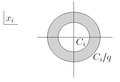
Figure 2: Illustration of integration contour

So, in order for (27) to hold, we must be able to shrink the contour $C_{i}/q$ back to $C_{i}$ so that we can take the sum over $i$ inside again.

We consider the implications of this condition in the following subsections.

4.2 From full derivative to shift operators in times

As we now have ensured that the insertions we consider are well-defined and vanishing, we will proceed with rewriting them as some difference operators acting on times $\{t_{k}\}$, in complete analogy with the non-$(q,t)$-deformed case.

4.2.1 The generic constraint

The integrand of the left hand side of (31) can be rewritten as (see Appendix B)

$$\sum\limits_{i=1}^{N}\ x_{i}^{\dagger}G_{i}(\underline{x})F(\underline{x})=\dfrac{F(\underline{x})}{(t-1)}\sum_{i=1}^{N}\operatorname*{Res}_{\omega=q/x_{i}}\dfrac{d\omega}{\omega-z}\frac{c_{q}(1/\omega)}{c_{q}(q/\omega)}\prod\limits_{j=1}^{N}\dfrac{q-t\omega x_{j}}{q-\omega x_{j}}\prod\limits_{k=1}^{M}\dfrac{\omega-ty_{k}}{\omega-y_{k}}~{},$$ (32)

After we integrate over the eigenvalues, the left hand side of (32) can be rewritten as

$$\begin{split}\oint_{C_{1}}\dots\oint_{C_{i}}\dots\oint_{C_{N}}\prod_{j=1}^{N}\frac{dx_{j}}{x_{j}}\sum_{i=1}^{N}x_{i}^{\dagger}G_{i}(\underline{x})F(\underline{x})=\oint_{C_{1}}\dots\oint_{C_{i}}\dots\oint_{C_{N}}\prod_{j=1}^{N}\frac{dx_{j}}{x_{j}}\sum_{i=1}^{N}G_{i}(\underline{x})F(\underline{x})\end{split}$$ (33)

provided we can shrink contour $C_{i}/q$ back to $C_{i}$. We can do this if there are no poles of the subintegral expression in the shaded region. Let’s look at different parts of the subintegral expression in detail.

As we said before, we treat the first part of $G_{i}(\underline{x})$, $\frac{1}{1-zx_{i}}$, as a formal power series in non-negative powers of $z$, therefore, it doesn’t contribute any poles. The second part of $G_{i}(\underline{x})$, $\prod_{j\neq i}\frac{x_{j}-tx_{i}}{x_{j}-x_{i}}$ , can possibly have poles at $x_{j}=x_{i}$ for $j\neq i$ which could appear in the shaded area. However, the $q$-Pochhammer in the numerator of $F(\underline{x})$, $\prod_{k\neq l}(x_{k}/x_{l};q)_{\infty}$ will precisely cancel these poles, and so there is no additional contribution from $G_{i}(\underline{x})$ as we shrink the contour.

Then let’s consider $F(\underline{x})$. The first part, $\prod_{k\neq l}\frac{(x_{k}/x_{l};q)_{\infty}}{(tx_{k}/x_{l};q)_{\infty}}$, can have poles for non-integer $\beta$. However, these poles are canceled by the numerator of $G_{i}(\underline{x})$. In the second part of $F(\underline{x})$, the function $c_{q}(x_{i})$ can, in principle, have poles in the shaded region. One therefore needs to show that this doesn’t happen for the model one is interested in, otherwise equation (27) would acquire a non-trivial right hand side.

For the $(q,t)$-Gaussian model, the function $c_{q}(x_{i})$ is given by (4) and does not pick up any poles as we shrink the contour from encircling $(-\nu/q,\ \nu/q)$ to encircling $(-\nu,\nu)$: indeed, the only possible pole in this area is the point $x=\nu/q$ (a pole of $f_{\lambda}$) but it coincides with a zero of the $q$-Gaussian measure $(x^{2}q^{2}\nu^{-2};q^{2})_{\infty}$ and therefore is just a regular point.

For the gauge theory on $D^{2}\times S^{1}$ model, the argument is analogous: for a given fugacity $m_{f}$ as we shrink the contour from encircling $(m_{f}^{-1}/q,\infty)$ to encircling $(m_{f}^{-1},\infty)$, we do not encounter any poles, provided other fugacities $m_{f^{\prime}}$ are in generic positions.

Having demonstrated that for these two models there are no contributions from poles in the shaded area, from now on we proceed assuming this is the case, so that

$$\oint\prod_{j=1}^{N}\frac{dx_{j}}{x_{j}}\sum\limits_{i=1}^{N}x_{i}^{\dagger}G_{i}(\underline{x})F(\underline{x})=\oint\prod_{j=1}^{N}\frac{dx_{j}}{x_{j}}\sum\limits_{i=1}^{N}G_{i}(\underline{x})F(\underline{x})~{}.$$

We then use the following algebraic identity (verified in Appendix C)

$$\sum\limits_{i=1}^{N}G_{i}(\underline{x})=\sum\limits_{i=1}^{N}\ \dfrac{1}{1-zx_{i}}\ \prod\limits_{j\neq i}\dfrac{x_{j}-tx_{i}}{x_{j}-x_{i}}=\frac{1}{1-t}-\frac{1}{1-t}\prod_{i=1}^{N}\frac{t-zx_{i}}{1-zx_{i}}$$ (34)

to obtain that

$$\begin{split}\oint\prod_{j=1}^{N}\frac{dx_{j}}{x_{j}}\sum\limits_{i=1}^{N}G_{i}(\underline{x})F(\underline{x})=\oint\prod_{j=1}^{N}\frac{dx_{j}}{x_{j}}&\bigg{\{}\frac{1}{1-t}-\frac{1}{1-t}\prod_{i=1}^{N}\frac{t-zx_{i}}{1-zx_{i}}\bigg{\}}F(\underline{x})~{}.\end{split}$$ (35)

Let’s now move to the right hand side of equation (32) where we also take an integral over eigenvalues. We want to interchange the integral over eigenvalues with operation of taking the residue. But we cannot do this, since the points we take residues at manifestly depend on the eigenvalues. Therefore, we change the sum over residues at $\omega=q/x_{i}$ for the sum of residues at $\omega=0$ and $\omega=\infty$ (details are in Appendix D). Then we can safely exchange integral over eigenvalues with the residue operator.

$$\begin{split}\frac{1}{(t-1)}&\oint\prod_{j=1}^{N}\frac{dx_{j}}{x_{j}}F(\underline{x})\sum_{i=1}^{N}\operatorname*{Res}_{\omega=q/x_{i}}\dfrac{d\omega}{\omega-z}\frac{c_{q}(1/\omega)}{c_{q}(q/\omega)}\prod\limits_{k=1}^{N}\dfrac{q-t\omega x_{k}}{q-\omega x_{k}}\prod\limits_{l=1}^{M}\dfrac{\omega-ty_{l}}{\omega-y_{l}}\\ &\emph{}=\left(-\operatorname*{Res}_{\omega=\infty}-\frac{1}{(t-1)}\operatorname*{Res}_{\omega=0}\right)\dfrac{d\omega}{\omega-z}\frac{c_{q}(1/\omega)}{c_{q}(q/\omega)}\prod\limits_{l=1}^{M}\dfrac{\omega-ty_{l}}{\omega-y_{l}}\oint\prod_{j=1}^{N}\frac{dx_{j}}{x_{j}}F(\underline{x})\prod\limits_{k=1}^{N}\dfrac{q-t\omega x_{k}}{q-\omega x_{k}}\end{split}$$ (36)

We can only do the above transformation provided that the subintegral expression has no other poles except $q/x_{i}$, $0$ and $\infty$. If there would be extra poles they would contribute to the right hand side of the Ward identities. Then Ward identities would no longer be $q$-Virasoro constraints, at least not in the representation (18). So, we have an additional requirement that $\frac{c_{q}(1/\omega)}{c_{q}(q/\omega)}$ should have no poles except at $0$ and $\infty$. This requirement should be checked for every concrete model one is interested in. For instance, for the $(q,t)$-Gaussian matrix model it is straightforward to see that this is, indeed, the case. For the gauge theory on $D^{2}\times S^{1}$, however, the fugacity for the fundamental, $m_{f}$, that appears in the denominator of (7) could cause such poles. Therefore, the dependence on the fundamental fugacities can be studied in the framework of $q$-Virasoro constraints only as a formal power series. Luckily, the dependence on the anti-fundamental fugacities $\bar{m}_{f}$ need not be understood formally, one can study it non-perturbatively.

Hence, equation (32) becomes (after some massaging that involves calculating residue at $\omega=\infty$)

$$\begin{split}\Bigg{[}\oint\prod_{j=1}^{N}\frac{dx_{j}}{x_{j}}&\bigg{\{}\frac{1}{1-t}-\frac{1}{1-t}\prod_{i=1}^{N}\frac{t-zx_{i}}{1-zx_{i}}\bigg{\}}F(\underline{x})-\frac{t^{N}}{(t-1)}\left.\frac{c_{q}(z)}{c_{q}(qz)}\right|_{z=0}\oint\prod_{i=1}^{N}\frac{dx_{i}}{x_{i}}F(\underline{x})\\ &\emph{}+\frac{1}{(t-1)}\oint_{\omega=0}\dfrac{d\omega}{\omega-z}\frac{c_{q}(1/\omega)}{c_{q}(q/\omega)}\prod\limits_{i=1}^{M}\dfrac{\omega-ty_{i}}{\omega-y_{i}}\oint\prod_{j=1}^{N}\frac{dx_{j}}{x_{j}}F(\underline{x})\prod\limits_{k=1}^{N}\dfrac{q-t\omega x_{k}}{q-\omega x_{k}}\Bigg{]}\ =\ 0~{}.\end{split}$$ (37)

Using the explicit form of the generating function given in (1) and the simple fact that $c_{q}(z)/c_{q}(qz)\big{|}_{z=0}=Q^{-1}p^{-1}q^{-\sqrt{\beta}\alpha}$ where $\alpha$ is the momentum parameter from (3), we can write the above in terms of the partition function $\mathcal{Z}$ using shifts in the time-variables $\{t_{k}\}$:

$$\boxed{\ \ \ \ \ \begin{split}&-\Bigg{(}p^{-1}q^{-\sqrt{\beta}\alpha}+1\Bigg{)}\ \mathcal{Z}\big{\{}t_{k}\big{\}}+t^{N}\mathcal{Z}\left\{t_{k}\rightarrow t_{k}+\frac{z^{k}}{k}(1-t^{-k})\right\}\\ &+\oint_{\omega=0}\frac{d\omega}{\omega-z}\ \frac{c_{q}(1/\omega)}{c_{q}(q/\omega)}\ e^{\sum_{k=1}^{\infty}\frac{(1-q^{k})t_{k}}{\omega^{k}}}\ \mathcal{Z}\left\{t_{k}\rightarrow t_{k}+\frac{\omega^{k}(1-t^{k})}{kq^{k}}\right\}=0~{},\end{split}\ \ \ \ \ }$$ (38)

which is then our first constraint equation.

Here we have rewritten certain products as exponents of logarithms, for instance

$$\prod_{i=1}^{M}\frac{\omega-ty_{i}}{\omega-y_{i}}=\exp\left(\sum_{k=1}^{\infty}\frac{(1-t^{k})}{\omega^{k}}\frac{\left(\sum_{i=1}^{M}y_{i}^{k}\right)}{k}\right)=\exp\left(\sum_{k=1}^{\infty}\frac{(1-q^{k})}{\omega^{k}}t_{k}\right);\ \ \ t_{k}=\frac{(1-q^{k})}{(1-t^{k})k}\sum_{i=1}^{M}y_{i}^{k}~{}.$$ (39)

Let us proceed to the second constraint.

4.2.2 The special additional constraint

There is another insertion of full $q$-derivative that one can consider, that leads to an additional equation for the partition function. In the case of $(q,t)$-deformed matrix model, this equation is necessary to make the system of equations closed and to be able to find all the correlators. In the classical limit this equation goes into the string equation. To obtain it, we begin with the relation (verified in Appendix B)

$$\sum\limits_{i=1}^{N}\ x_{i}^{\dagger}\tilde{G}_{i}(\underline{x})F(\underline{x})=\dfrac{F(\underline{x})}{(t-1)}\sum_{i=1}^{N}\operatorname*{Res}_{\omega=q/x_{i}}d\omega\frac{c_{q}(1/\omega)}{c_{q}(q/\omega)}\prod\limits_{j=1}^{N}\dfrac{q-t\omega x_{j}}{q-\omega x_{j}}\prod\limits_{k=1}^{M}\dfrac{\omega-ty_{k}}{\omega-y_{k}},$$ (40)

where now

$$\tilde{G}_{i}(\underline{x})=\dfrac{1}{x_{i}}\ \prod\limits_{j\neq i}\dfrac{x_{j}-tx_{i}}{x_{j}-x_{i}}~{}.$$ (41)

Proceeding similarly to above, the first step is to take a contour integral of the left hand side and use the algebraic identity

$$\sum\limits_{i=1}^{N}\tilde{G}_{i}(\underline{x})=\sum\limits_{i=1}^{N}\ \dfrac{1}{x_{i}}\ \prod\limits_{j\neq i}\dfrac{x_{j}-tx_{i}}{x_{j}-x_{i}}=\sum\limits_{i=1}^{N}\dfrac{1}{x_{i}}$$ (42)

to get

$$\oint\prod_{j=1}^{N}\frac{dx_{j}}{x_{j}}\sum\limits_{i=1}^{N}x_{i}^{\dagger}\tilde{G}_{i}(\underline{x})F(\underline{x})=\oint\prod_{j=1}^{N}\frac{dx_{j}}{x_{j}}\bigg{\{}\sum\limits_{i=1}^{N}\dfrac{1}{x_{i}}\bigg{\}}F(\underline{x})~{}.$$ (43)

We then transform the right hand side by changing the residues from $\omega=q/x_{i}$ to $0$ and $\infty$ and swapping integration over eigenvalues with taking the residue. Writing the result using $\mathcal{Z}\{t_{k}\}$ we get after some calculation

$$\boxed{\ \ \ \ \ \begin{split}\oint&\prod_{j=1}^{N}\frac{dx_{j}}{x_{j}}\bigg{\{}\sum\limits_{i=1}^{N}\dfrac{1}{x_{i}}\bigg{\}}F(\underline{x})\Bigg{(}1-q^{-\sqrt{\beta}\alpha}\Bigg{)}+q^{-\sqrt{\beta}\alpha}\ \mathcal{Z}\big{\{}t_{k}\big{\}}t_{1}\frac{(1-q)}{(1-t)}\\ &+\frac{1}{(t-1)}\operatorname*{Res}_{\omega=0}d\omega\frac{c_{q}(1/\omega)}{c_{q}(q/\omega)}e^{\sum_{k=1}^{\infty}\frac{(1-q^{k})t_{k}}{\omega^{k}}}\mathcal{Z}\left\{t_{k}\rightarrow t_{k}+\frac{\omega^{k}(1-t^{k})}{kq^{k}}\right\}=0~{}.\end{split}\ \ \ \ \ }$$ (44)

Note that the complicated first term vanishes in the case $\alpha=0$; this will be useful later. Otherwise, it is not clear what to do with it: it is an average of $\langle\text{tr}X^{-1}\rangle$ and as such it is not expressible as any differential operator in $\{t_{k}\}$ acting on $\mathcal{Z}$. Perhaps, the set of times could be enlarged to be able to also generate correlators of traces of negative powers of $X$, however, investigation of this possibility is beyond the scope of the present paper.

4.2.3 Combining generic and special constraints

We then want to combine our two constraint equations. The key point here is the observation that the first constraint in equation (38) can be written as

$$\begin{split}&\Bigg{(}p^{-1}q^{-\sqrt{\beta}\alpha}+1\Bigg{)}\ \mathcal{Z}\big{\{}t_{k}\big{\}}-t^{N}\mathcal{Z}\left\{t_{k}\rightarrow t_{k}+\frac{z^{k}}{k}(1-t^{-k})\right\}\\ &=\frac{c_{q}(1/z)}{c_{q}(q/z)}\ e^{\sum_{k=1}^{\infty}\frac{(1-q^{k})t_{k}}{z^{k}}}\ \mathcal{Z}\left\{t_{k}\rightarrow t_{k}+\frac{z^{k}(1-t^{k})}{kq^{k}}\right\}+f(1/z)\end{split}$$ (45)

for some function $f(1/z)=\sum_{m=1}^{\infty}\frac{d_{m}}{z^{m}}$ containing only negative powers in $z$. The second constraint equation in (44) then gives us the coefficient of $\frac{1}{z}$ in this series, allowing to combine into

$$\boxed{\ \ \ \begin{split}t^{N}&\mathcal{Z}\left\{t_{k}\rightarrow t_{k}+\frac{z^{k}}{k}(1-t^{-k})\right\}\ +\ \frac{c_{q}(1/z)}{c_{q}(q/z)}\ e^{\sum_{k=1}^{\infty}\frac{(1-q^{k})t_{k}}{z^{k}}}\ \mathcal{Z}\left\{t_{k}\rightarrow t_{k}+\frac{z^{k}(1-t^{k})}{kq^{k}}\right\}\\ &=\big{(}p^{-1}q^{-\sqrt{\beta}\alpha}+1\big{)}\ \mathcal{Z}\big{\{}t_{k}\big{\}}+\frac{1-t}{z}\oint\prod_{j=1}^{N}\frac{dx_{j}}{x_{j}}\bigg{\{}\sum\limits_{i=1}^{N}\dfrac{1}{x_{i}}\bigg{\}}F(\underline{x})\Bigg{\{}1-q^{-\sqrt{\beta}\alpha}\Bigg{\}}\\ &+\frac{1-q}{z}\ p^{-1}q^{-\sqrt{\beta}\alpha}\ t_{1}\mathcal{Z}\big{\{}t_{k}\big{\}}+\sum_{m=2}^{\infty}\frac{d_{m}}{z^{m}}\end{split}\ \ \ \ \ }$$ (46)

which the generating function $\mathcal{Z}\{t_{k}\}$ must satisfy.

As an example and for comparison with earlier work on $q$-Virasoro, let us consider the special case with no potential, i.e. $N_{f}=0$ and $\alpha=0$. It can be seen that in this case the above constraint takes a simple form

$$\begin{split}t^{N}\mathcal{Z}\{t_{k}\rightarrow t_{k}+\frac{z^{k}}{k}(1-t^{-k})\}+&q^{-1}t^{1-N}e^{\sum_{k=1}^{\infty}\frac{(1-q^{k})t_{k}}{z^{k}}}\mathcal{Z}\{t_{k}\rightarrow t_{k}+\frac{z^{k}(1-t^{k})}{kq^{k}}\}\\ =&(p^{-1}+1)\mathcal{Z}\{t_{k}\}+\frac{tq^{-1}(1-q)t_{1}\mathcal{Z}\{t_{k}\}}{z}+\sum_{m=2}^{\infty}\frac{c_{m}}{z^{m}}~{},\end{split}$$ (47)

for some coefficients $c_{m}$. Comparing this to the construction in Shiraishi:1995rp and the $q$-Virasoro constraint in equation (23) (with $z\rightarrow 1/z$) we are considering

$$\psi(1/z)T(1/z)\mathcal{Z}\{t_{k}\}=c_{0}+\frac{c_{1}}{z}+\sum_{m=2}^{\infty}\frac{c_{m}}{z^{m}}$$ (48)

with $c_{0}$ and $c_{1}$ being the coefficients of the $z^{0}$ and $z^{-1}$ terms respectively, and

$$\psi(1/z)=p^{-\frac{1}{2}}\exp\left\{\sum_{k>0}^{\infty}\frac{(1-q^{k})t_{k}}{(1+p^{k})z^{k}}\right\}~{}.$$ (49)

To then extract the action of $T_{0}$ and $T_{-1}$ on $\mathcal{Z}\{t_{k}\}$ we expand the stress tensor current $T(1/z)=\sum_{n\in\mathbb{Z}}T_{n}z^{n}$ and compute

$$\begin{split}T(1/z)\mathcal{Z}\{t_{k}\}=&\psi(1/z)^{-1}\left((p^{-1}+1)\mathcal{Z}\{t_{k}\}+\frac{tq^{-1}(1-q)t_{1}\mathcal{Z}\{t_{k}\}}{z}+\sum_{m=2}^{\infty}\frac{c_{m}}{z^{m}}\right)\\ =&\left(p^{\frac{1}{2}}+p^{-\frac{1}{2}}\right)\mathcal{Z}\{t_{k}\}+\psi(1/z)^{-1}\left(\sum_{m=2}^{\infty}\frac{c_{m}}{z^{m}}\right)\end{split}$$ (50)

from which we can identify the eigenvalue equations

$$\begin{split}T_{0}\mathcal{Z}\{t_{k}\}=&\left(p^{\frac{1}{2}}+p^{-\frac{1}{2}}\right)\mathcal{Z}\{t_{k}\}\\ T_{-1}\mathcal{Z}\{t_{k}\}=&0~{}.\end{split}$$ (51)

This can also be obtained using the free field representation of Nedelin:2016gwu as shown in appendix E, and so these two viewpoints are equivalent.

5 Recursive solution

The aim of this section is to show how $q$-Virasoro constraints can be used to recursively determine all normalized correlators of a given eigenvalue model. We will use the $(q,t)$-Gaussian matrix model as an example, but models with more involved potentials can be treated similarly – they just require more initial conditions to start the recursion. This situation is completely analogous to the usual, non-$(q,t)$-deformed case, where one needs to choose a set of integration contours (i.e. the “phase” of the model) to define its correlators Cordova:2016jlu .

The $q$-Virasoro constraints (46), specialized for $(q,t)$-Gaussian matrix model, read

$$tQ^{-1}\left(1-q^{2}(1-q)y^{2}\right)\exp\left(\sum_{k=1}^{\infty}(1-q^{k})t_{k}y^{k}\right)\mathcal{Z}\left\{t_{k}\rightarrow t_{k}+\frac{(1-t^{k})}{kq^{k}}\frac{1}{y^{k}}\right\}$$ (52)

$$+qQ\mathcal{Z}\left\{t_{k}\rightarrow t_{k}+\frac{(1-t^{-k})}{k}\frac{1}{y^{k}}\right\}-(q+t)\mathcal{Z}\left\{t_{k}\right\}-yt(1-q)t_{1}\mathcal{Z}\left\{t_{k}\right\}=\sum_{m=0}^{\infty}c_{m}y^{m+2}$$

where $Q=t^{N}$ and $c_{m}$ are coefficients of the expansion in $y$. We search for a formal power series solution to this equation

$$\mathcal{Z}\{t_{k}\}=\sum_{n=0}^{\infty}\frac{1}{n!}\sum_{d=0}^{\infty}\sum_{l_{1}+\dots+l_{n}=d}C_{l_{1}\dots l_{n}}t_{l_{1}}\dots t_{l_{n}}=\sum_{d=0}^{\infty}\mathcal{Z}_{d}\{t_{k}\},$$ (53)

where $C_{l_{1}\dots l_{n}}$ are correlators. $\mathcal{Z}_{d}\{t_{k}\}$ is defined to be the degree $d$ component of the partition function with respect to the action of the operator $\sum_{d=1}^{\infty}d\;t_{d}\frac{\partial}{\partial t_{d}}$.

Extracting the coefficient in front of $y^{-m},m=-1,0,1,...$ and of particular degree $d$ in times $t_{n}$ from equation (52) we get

$$tQ^{-1}q^{2}(1-q)s_{m+2}\left(\left\{p_{k}=\frac{(1-t^{k})}{q^{k}}\frac{\partial}{\partial t_{k}}\right\}\right)\mathcal{Z}_{d+2}\{t_{k}\}$$ (54)

$$=tQ^{-1}s_{m}\left(\left\{p_{k}=\frac{(1-t^{k})}{q^{k}}\frac{\partial}{\partial t_{k}}\right\}\right)\mathcal{Z}_{d}\{t_{k}\}$$

$$\quad+qQ\sum_{p=0}^{d-m}s_{p}\left(\left\{p_{k}=-(1-q^{k})kt_{k}\right\}\right)s_{p+m}\left(\left\{p_{k}=(1-t^{-k})\frac{\partial}{\partial t_{k}}\right\}\right)\mathcal{Z}_{d}\{t_{k}\}$$

$$\quad-\delta_{m,0}(q+t)\mathcal{Z}_{d}\{t_{k}\}+\delta_{m,-1}q(1-q)t_{1}\mathcal{Z}_{d}\{t_{k}\},$$

where $s_{m}(p_{1},\dots,p_{m})$ is Schur polynomial for symmetric representation $[m]$, see (LABEL:eq:symm-schur-poly).

By considering coefficients in front of all monomials in times $t_{n}$ in equations (54), we obtain an overdetermined system of linear equations for the correlators $C_{l_{1}\dots l_{n}}$. From this system one can actually pick certain equations in a clever way in specific order and obtain a recursive formula for the correlators. Suppose we wish to find the correlator $C_{\lambda_{1}...\lambda_{\bullet-1}\lambda_{\bullet}}$. Here $\lambda_{\bullet}$ means the last part of the partition $\lambda$ and we assume that indices of the correlator are sorted in descending order such that $\lambda_{\bullet}$ is the smallest index (the correlator is of course symmetric as a function of its indices). We then consider equation (54) with $m+2=\lambda_{\bullet},\ \ d+2=|\lambda|$ and apply $\Bigg{|}_{\vec{t}=0}\frac{\partial^{\bullet-1}}{\partial t_{\lambda_{1}}\dots\partial t_{\lambda_{\bullet-1}}}$ to it (i.e. setting all times to zero after taking the partial derivative). We then get

$$tQ^{-1}q^{2}(1-q)\frac{1}{\lambda_{\bullet}} \frac{(1-t^{\lambda_{\bullet}})}{q^{\lambda_{\bullet}}}C_{\lambda_{1}\dots\lambda_{\bullet}}=-tQ^{-1}q^{2}(1-q)\sum_{\begin{subarray}{c}|\vec{\mu}|=\lambda_{\bullet}\\ l(\vec{\mu})\geq 2\end{subarray}}\frac{1}{l(\vec{\mu})!}\left(\prod_{a\in\vec{\mu}}\frac{(1-t^{a})}{q^{a}a}\right)C_{\lambda_{1}\dots\lambda_{\bullet-1}\mu_{1}\dots\mu_{\bullet}}$$ (55)

$$-\delta_{\lambda_{\bullet},2}(q+t)C_{\lambda_{1}\dots\lambda_{\bullet-1}}+\delta_{\lambda_{\bullet},1}((\#_{\lambda}1)-1)q(1-q)C_{\lambda_{1}\dots\lambda_{\bullet-2}}$$

$$+tQ^{-1}\sum_{|\vec{\mu}|=\lambda_{\bullet}-2}\frac{1}{l(\vec{\mu})!}\left(\prod_{a\in\vec{\mu}}\frac{(1-t^{a})}{q^{a}a}\right)C_{\lambda_{1}\dots\lambda_{\bullet-1}\mu_{1}\dots\mu_{\bullet}}$$

$$+qQ\sum_{\nu\subseteq\lambda\setminus\lambda_{\bullet}}\left(\prod_{a\in\nu}(-1)(1-q^{a})\right)\sum_{|\vec{\mu}|=|\nu|+\lambda_{\bullet}-2}\frac{1}{l(\vec{\mu})!}\left(\prod_{a\in\vec{\mu}}\frac{(1-t^{-a})}{a}\right)C_{\lambda\setminus\{\lambda_{\bullet},\nu\}\vec{\mu}}$$

Here $\vec{\mu}$ denotes an ordered sequence of positive integer numbers (it can be an empty sequence), as opposed to a partition which is sorted sequence of positive integer numbers and $l(\vec{\mu})$ is the length of the sequence $\vec{\mu}$. $\#_{\lambda}1$ is the number of parts of $\lambda$ equal to 1, $\lambda\setminus\lambda_{\bullet}$ is partition $\lambda$ without part $\lambda_{\bullet}$ and $\lambda\setminus\{\lambda_{\bullet},\nu\}$ is partition $\lambda$ with part $\lambda_{\bullet}$ and all parts of $\nu$ removed.

The formula (55) is indeed a recursion: correlators on all lines of the right hand side except the first one have sum of indices equal to $|\lambda|-2$; the correlators on the first line, though having sum of indices equal to $|\lambda|$, all have a minimal index that is strictly less than $\lambda_{\bullet}$ (thanks to the condition $l(\vec{\mu})\geq 2$).

Supplemented with the initial conditions $C_{\emptyset}=1$ and $C_{1}=0$, this recursion allows us to calculate any particular correlator in a finite number of steps.

Example:

The first step of the recursion looks like

$$tQ^{-1}q^{2}(1-q)\frac{(1-t)}{q}C_{1,1} =q(1-q)+qQ(-1)(1-q)$$ (56)

$$\Longrightarrow C_{1,1}=\frac{Q(1-Q)}{t(1-t)}$$

$$tQ^{-1}q^{2}(1-q)\frac{1}{2}\frac{(1-t^{2})}{q^{2}}C_{2} =-tQ^{-1}q^{2}(1-q)\frac{1}{2}\frac{(1-t)^{2}}{q^{2}}C_{1,1}-(q+t)+tQ^{-1}\frac{1}{0!}+qQ$$

$$\Longrightarrow C_{2}=\frac{(1-Q)(2t-Q-qQ+tQ-qtQ)}{t(1-q)(1-t^{2})}$$

In the case of non-$(q,t)$-deformed Hermitean matrix model, the Virasoro constraints can be used to derive the so-called $\hat{W}$-operator representation of the partition function Morozov:2009xk . This derivation can be easily generalized to the case of Gaussian $\beta$-ensemble. However, at the moment we do not know how to generalize it to the $(q,t)$-Gaussian matrix model, as well as more complicated $(q,t)$-models. Existence of $\hat{W}$-operator form (the cut-and-join equation) is intimately linked with the existence of the spectral curve topological recursion for the model Eynard:2007kz ; Alexandrov:2006qx ; Alexandrov:2009gn ; Orantin:2008hq and often signifies connections with enumerative geometry doi:10.1112/jlms/jdv047 . Pursuing these directions is definitely worth it in the future.

6 Gauge theory applications

From the point of view of gauge theories the normalized correlators $C_{l_{1}\dots l_{n}}$ are not very interesting. Instead, of primary interest are averages of Schur functions, which on the gauge theory side correspond to supersymmetric Wilson loops (see Nedelin:2016gwu and references therein). In the gauge theory on $D^{2}\times S^{1}$ the expectation value of the Wilson loop along $S^{1}$ in representation $\lambda$ corresponds to the following expression

$$\left\langle s_{\lambda}\right\rangle=\oint_{c}\prod_{i=1}^{N}\frac{dx_{i}}{x_{i}}\prod_{k\neq l=1}^{N}\frac{(x_{k}/x_{l};q)_{\infty}}{(tx_{k}/x_{l};q)_{\infty}}\ \prod_{j=1}^{N}\prod_{f=1}^{N_{f}}\frac{(qx_{j}\overline{m}_{f};q)_{\infty}}{(x_{j}m_{f};q)_{\infty}}\ s_{\lambda}(x)~{},$$ (57)

where $s_{\lambda}$ is Schur polynomial for the representation $\lambda$. If we choose $N_{f}=2$ with two opposite anti-fundamental masses $\pm\overline{m}$ having the special values $\pm\overline{m}_{f}=\pm q(1-q)^{\frac{1}{2}}$ and without fundamental contributions we can use the previously derived results. This choice of masses is by no means distinguished from the gauge theory point of view. Moreover, one could easily insert arbitrary values of the two anti-fundamental masses on the matrix model side as well, and this will not complicate $q$-Virasoro constraints at all (the factor $\left(1-q^{2}(1-q)y^{2}\right)$ in the first term of the equation (52) will be replaced by $\left(1-\overline{m}_{1}y\right)\left(1-\overline{m}_{2}y\right)$ but it will still remain quadratic, so non-Gaussian issues will still not arise). In what follows we present formulas at special values of the masses for conciseness.

Reexpanding the partition function in the basis of Schur functions (using Cauchy identity)

$$\mathcal{Z}\{t_{k}\}=\sum_{n=0}^{\infty}\frac{1}{n!}\sum_{l_{1},\dots,l_{n}}C_{l_{1}\dots l_{n}}t_{l_{1}}\dots t_{l_{n}}=\left\langle\exp\left(\sum_{k=1}^{\infty}\text{tr}\Phi^{k}t_{k}\right)\right\rangle=\sum_{\lambda}s_{\lambda}(\{p_{k}=kt_{k}\})\left\langle s_{\lambda}(\{p_{k}=\text{tr}\Phi^{k}\})\right\rangle$$ (58)

it is straightforward to obtain constraints on Schur averages. In the case of the $(q,t)$-Gaussian model, the first few of them are:

$$\left\langle s_{2}\right\rangle=\left\langle s_{\emptyset}\right\rangle\Bigg{(} Q^{2}\left(\frac{-5q-3}{2(q-1)t}+\frac{5q-1}{2(q-1)(t-1)}+\frac{2}{(q-1)(t+1)}\right)$$ (59)

$$+Q\left(\frac{-5q-3}{2(q-1)(t-1)}+\frac{5q+3}{2(q-1)t}\right)+\frac{2}{(q-1)(t-1)}-\frac{2}{(q-1)(t+1)}\Bigg{)}$$

$$\left\langle s_{1,1}\right\rangle=\left\langle s_{\emptyset}\right\rangle\Bigg{(} Q^{2}\left(\frac{-3q-1}{2(q-1)(t-1)}+\frac{3q+5}{2(q-1)t}-\frac{2}{(q-1)(t+1)}\right)$$

$$+Q\left(\frac{-3q-5}{2(q-1)t}+\frac{3q+5}{2(q-1)(t-1)}\right)-\frac{2}{(q-1)(t-1)}+\frac{2}{(q-1)(t+1)}\Bigg{)}$$

$$\left\langle s_{4}\right\rangle=\left\langle s_{2}\right\rangle \Bigg{(}\Big{(}\frac{-59q-21}{8(q-1)t}+\frac{7q-3}{8(q-1)(t-1)}+\frac{8q+9}{2(q-1)(t+1)}+\frac{-6q^{2}+5tq-5q-3t-5}{2(q-1)\left(t^{2}+1\right)}$$

$$\quad\quad+\frac{1205q^{3}+801q^{2}+855q+211}{192(q-1)t^{2}}+\frac{-241q^{3}-117q^{2}-27q+1}{64(q-1)t^{3}}\Big{)}Q^{2}$$

$$\quad+\left(\frac{-7q-1}{8(q-1)(t-1)}-\frac{21}{8t}+\frac{4}{t+1}+\frac{-tq+5q+3t-7}{2(q-1)\left(t^{2}+1\right)}\right)Q$$

$$\quad+\frac{1}{2(q-1)(t-1)}-\frac{17}{2(q-1)(t+1)}+\frac{8t-1}{(q-1)\left(t^{2}+1\right)}\Bigg{)}$$

$$+\left\langle s_{1,1}\right\rangle \Bigg{(}\Big{(}\frac{1-5q}{8(q-1)(t-1)}-\frac{3(13q+3)}{8(q-1)t}+\frac{8q+7}{2(q-1)(t+1)}+\frac{-10q^{2}+3tq-3q-5t-3}{2(q-1)\left(t^{2}+1\right)}$$

$$\quad\quad+\frac{241q^{3}+445q^{2}+267q+71}{64(q-1)t^{2}}-\frac{5\left(241q^{3}+117q^{2}+27q-1\right)}{192(q-1)t^{3}}\Big{)}Q^{2}$$

$$\quad+\left(\frac{5q+3}{8(q-1)(t-1)}-\frac{9}{8t}+\frac{4}{t+1}+\frac{-7tq+3q+5t-1}{2(q-1)\left(t^{2}+1\right)}\right)Q$$

$$-\frac{1}{2(q-1)(t-1)}-\frac{15}{2(q-1)(t+1)}+\frac{8t+1}{(q-1)\left(t^{2}+1\right)}\Bigg{)}$$

These expressions are examples of the expectation values of Wilson loops in $D^{2}\times S^{1}$ with the specific choices for the matter sector. In principle one may obtain the formulas for general values of fundamental mass by using the shifts in times. At the moment we do not know of a more direct way to write down the expessions of the form (59). Moreover, in the case of usual, non-$(q,t)$-deformed matrix models the Virasoro constraints look rather cumbersome in the Schur basis Adler2003 so there is no reason to expect them to be simpler for the $(q,t)$-deformation.

It is curious that from the point of view of $(q,t)$-deformed matrix models it is natural to study averages not of Schur functions, but rather of Macdonald functions ${\cal M}_{\lambda}(\{p_{k}\})$ Morozov:2018eiq . Computer experiments show that in many examples Macdonald averages have a very simple, explicit form. For instance, for $(q,t)$-Gaussian matrix model one has

$$\left\langle{\cal M}_{\lambda}\right\rangle={\cal M}_{\lambda}\left(\left\{p_{k}=(1+(-1)^{k})\frac{(1-q)^{k/2}}{(1-t^{k})}\right\}\right)\prod_{(i,j)\in\lambda}\frac{1-t^{N+1-i}q^{j-1}}{1-q}$$ (60)

though at the moment we do not know how to prove this formula. But, at least in principle, Schur averages could be obtained from the vector of Macdonald averages by applying the inverse matrix of $(q,t)$-Kostka coefficients qtKostka .

The techniques suggested in this work can be combined with the free field realization of the gauge theory on squashed $S^{3}_{(\omega_{1},\omega_{2})}$ Nedelin:2016gwu . There exists the generating function for the expectation values of supersymmetric Wilson loops

$$\mathcal{Z}\{t_{k},\tilde{t}_{k}\}=\int_{i\mathbb{R}^{N}}\prod_{i=1}^{N}dX_{i}\prod_{k\neq l=1}^{N}\frac{S_{2}(X_{k}-X_{l}|\underline{\omega})}{S_{2}(M_{a}+X_{k}-X_{l}|\underline{\omega})}e^{\sum\limits_{j=1}^{N}V(X_{j})}e^{[\sum\limits_{n=0}^{\infty}t_{n}\sum\limits_{j=1}^{N}e^{2\pi inX_{j}/\omega_{1}}+\sum\limits_{n=0}^{\infty}\tilde{t}_{n}\sum\limits_{j=1}^{N}e^{2\pi inX_{j}/\omega_{2}}]}~{},$$ (61)

here we use the notations from Nedelin:2016gwu . Upon certain assumptions this generating function satisfies two commuting sets of $q$-Virasoro constraints. It is straightforward to repeat the analysis from Section 4.1 keeping in mind that there is a change of variables $x=e^{2\pi iX/\omega_{1}}$ (or $x=e^{2\pi iX/\omega_{2}}$ for another copy of $q$-Virasoro). We leave this analysis for future studies.

7 Conclusion

In this paper we showed how to derive the set of Ward identities which a $(q,t)$-eigenvalue model satisfies, starting from an integral representation of it. The derivation is based on a clever insertion of a full $q$-derivative under the integral. Under certain mild assumptions (which are to be checked in each particular case) these Ward identities are nothing but $q$-Virasoro constraints, which before could be derived only if the free field realization (in particular, the corresponding screening current) for the model was known.

The advantage of the method we present here is that it can be applied to any $(q,t)$-eigenvalue model directly – there is no need to know the free field representation beforehand. Hence, the situation with $(q,t)$-eigenvalue models now becomes very similar to the situation with $\beta$-ensembles, where Virasoro constraints can be derived both from free field realization and from insertion of full derivatives under the integral. We think that having these two complementary perspectives is useful, as each of them highlights different aspects of the eigenvalue models.

It is worth noting that from the $q$-derivative insertion method one quite naturally obtains more constraints than from free field realization. Namely, there is an additional constraint $T_{-1}\mathcal{Z}=0$. During its derivation one has to demand that the coefficient in front of $\left\langle\text{tr}X^{-1}\right\rangle$ vanishes, so that one stays in the usual setting of matrix models. On the free field representation side this extra equation is satisfied if one restricts attention to highest weights with zero momentum and it is very easy to overlook this special case.

There are several directions of further research that we think are interesting:

• Application to concrete matrix models: The $q$-Virasoro constraints (46) can be viewed as a definition of the matrix model. A particular integral representation is then just one instance (or “phase”) that satisfies this definition. It would be very interesting to study alternative phases of several objects which are of crucial importance in mathematical physics and are known to satisfy $q$-Virasoro constraints, such as ABJ(M) model and Nekrasov functions.

• $\hat{W}$-operator representation: In the case of usual Hermitean Gaussian matrix model the $\hat{W}$-operator representation is a consequence of Virasoro constraints. We hope that the explicit form of $q$-Virasoro constraints (55) will be useful in deriving $\hat{W}$-operator representation for the $(q,t)$-Gaussian model. The $\hat{W}$-operator representation would then readily imply connection to enumerative geometry.

• Large $N$ limit and related questions: For non-$(q,t)$-deformed matrix models the Virasoro constraints can be used to derive the so-called loop equations, which then may be solved in the large $N$ limit Eynard:2008we . A particular solution, satisfying certain mild assumptions, takes the form of a certain universal recursion procedure, the spectral curve topological recursion. Information about the concrete matrix model is translated into the initial algebrogeometric data for the recursion – the spectral curve. The spectral curve topological recursion is related to the Givental formalism for Cohomological field theories. It would be very interesting to see what the $(q,t)$-spectral curve topological recursion and $(q,t)$-Givental formalism look like.

• Relation to Macdonald operators: The $q$-difference operators that we insert under the integral look very similar to the celebrated Macdonald operators (Shiraishi:1995rp, , equation (31)). By understanding this connection better one could, perhaps, better understand the integrability of $(q,t)$-eigenvalue models.

We hope that these questions would inspire some great future research.

Acknowledgements: We thank Fabrizio Nieri for discussions. The work of RL, AP and MZ is supported in part by Vetenskapsrådet under grant #2014-5517, by the STINT grant, and by the grant “Geometry and Physics” from the Knut and Alice Wallenberg foundation. AP is also partially supported by RFBR grants 16-01-00291, 18-31-20046 mol_a_ved and 19-01-00680 A. SS is partially supported by RFBR grant 18-31-20046 mol_a_ved.

Appendix A Special functions

A summary of the special functions used throughout the paper. The definition of the $q$-Pochhammer symbol is

$$(x;q)_{\infty}=e^{-\sum_{k>0}\frac{x^{k}}{k(1-q^{k})}}=\prod_{k=0}^{\infty}(1-xq^{k})$$ (62)

valid for $|q|<1$, and the finite $q$-Pochhammer is given by

$$(x;q)_{n}=\frac{(x;q)_{\infty}}{(q^{n}x;q)_{\infty}}=\prod_{k=1}^{n-1}(1-xq^{k}).$$ (63)

The $\theta$ function is defined by

$$\theta(x;q)=(x;q)_{\infty}(qx^{-1};q)_{\infty}~{}.$$ (64)

The Schur polynomial $s_{m}(p_{1},\dots,p_{m})$ in symmetric representation $[m]$ is given by

$$\begin{split}&\exp\left(\sum_{k=1}^{\infty}\frac{z^{k}p_{k}}{k}\right)=\sum_{m=0}^{\infty}z^{m}s_{m}(p_{1},\dots,p_{m})\\ &s_{m}(p_{1},\dots,p_{m})=\prod_{\lambda\vdash m}\prod_{i=1}^{l(\lambda)}\frac{p_{i}}{i}\prod_{j=1}^{\infty}\frac{1}{(\#_{\lambda}j)!},\end{split}$$ (65)

where $\#_{\lambda}j$ is the number of parts $j$ in partition $\lambda$ and $l(\lambda)$ is the length of partition $\lambda$.

The $q$-integral is defined as

$$\int_{-\nu}^{\nu}d_{q}xg(x)=(1-q)\sum_{n=0}^{\infty}\nu q^{n}[g(\nu q^{n})+g(-\nu q^{n})]$$ (66)

with $\nu=(1-q)^{-\frac{1}{2}}$. For a $q$-shifted function $x^{\dagger}g(x)=g(x/q)$, provided $g(x)$ vanish at the boundary the $q$-shift can be rescaled away

$$\int\limits_{-\nu}^{\nu}g(x/q)\ d_{q}x=q\int\limits_{-\nu}^{\nu}g(x)\ d_{q}x.$$ (67)

One can also produce the $q$-integral by insertion of the operator $\mathcal{O}_{\nu}(x_{i})$,

$$\mathcal{O}_{\nu}(x_{i})=(1-q)\Bigg{\{}-\frac{(q;q)_{\infty}^{2}}{\theta(q^{\lambda};q)}\left[f_{\lambda}(x_{i}/\nu;q)-f_{\lambda}(-x_{i}/\nu;q)\right]\Bigg{\}}x_{i}$$ (68)

with

$$f_{\lambda}(x;q)=x^{\lambda}\ \frac{\theta(q^{\lambda}x;q)}{\theta(x;q)}~{},$$ (69)

which has the desired pole structure provided the choice of contours in figure 1. This can be seen using (66):

$$\begin{split}\oint_{C_{j}}\prod_{j=1}^{N}\frac{dx_{j}}{x_{j}}\prod_{i=1}^{N}\mathcal{O}_{\nu}(x_{i})g(\underline{x})=&\oint_{C_{j}}\prod_{j=1}^{N}\frac{dx_{j}}{x_{j}}\prod_{i=1}^{N}(1-q)\Bigg{\{}-\frac{(q;q)_{\infty}^{2}}{\theta(q^{\lambda};q)}\left[f_{\lambda}(x_{i}/\nu;q)-f_{\lambda}(-x_{i}/\nu;q)\right]\Bigg{\}}x_{i}g(\underline{x})\\ =&(1-q)^{N}\sum_{n=0}\nu q^{n}\left[g(\nu q^{n})+g(-\nu q^{n})\right]\\ =&\int_{-\nu}^{\nu}\prod_{i=1}^{N}d_{q}x_{i}g(\underline{x}).\end{split}$$ (70)

The $q$-exponent has (at least) two definitions

$$\begin{split}e_{q}(x_{i})=&\sum_{n=0}^{\infty}\frac{x_{i}^{n}}{[n]_{q}!}\\ =&\prod_{k=0}^{\infty}(1-(1-q)q^{k}x_{i})^{-1}.\end{split}$$ (71)

Appendix B Verification of starting relation

B.1 First starting relation

The starting relation (32)

$$\sum\limits_{i=1}^{N}\ x_{i}^{\dagger}G_{i}(\underline{x})F(\underline{x})=\dfrac{F(\underline{x})}{(t-1)}\sum_{i=1}^{N}\operatorname*{Res}_{\omega=q/x_{i}}\dfrac{d\omega}{\omega-z}\frac{c_{q}(1/\omega)}{c_{q}(q/\omega)}\prod\limits_{j=1}^{N}\dfrac{q-t\omega x_{j}}{q-\omega x_{j}}\prod\limits_{k=1}^{M}\dfrac{\omega-ty_{k}}{\omega-y_{k}}$$ (72)

can be checked as follows. For the left hand side

$$\begin{split}\sum_{i=1}^{N}x_{i}^{\dagger}G_{i}(\underline{x})F(\underline{x})=&\sum_{i=1}^{N}\frac{1}{1-zx_{i}/q}\prod_{j\neq i}\frac{x_{j}-tx_{i}/q}{x_{j}-x_{i}/q}\prod_{i\neq l}\frac{(x_{i}/(qx_{l});q)_{\infty}}{(tx_{i}/(qx_{l});q)_{\infty}}\prod_{k\neq l,k\neq i}\frac{(x_{k}/x_{l};q)_{\infty}}{(tx_{k}/x_{l};q)_{\infty}}\\ &\times\prod_{k\neq i}\frac{(qx_{k}/x_{i};q)_{\infty}}{(qtx_{k}/x_{i};q)_{\infty}}\prod_{k\neq l,l\neq i}\frac{(x_{k}/x_{l};q)_{\infty}}{(tx_{k}/x_{l};q)_{\infty}}e^{\sum_{k=1}^{\infty}t_{k}\left((x_{i}/q)^{k}+\sum_{j=1,j\neq i}^{N}x_{j}^{k}\right)}\\ &\times c_{q}(x_{i}/q)\prod_{j=1,j\neq i}^{N}c_{q}(x_{j})\\ =&F(\underline{x})\sum_{i=1}^{N}\frac{1}{1-zx_{i}/q}\prod_{j\neq i}\frac{(1-tx_{j}/x_{i})}{(1-x_{j}/x_{i})}e^{\sum_{k=1}^{N}t_{k}x_{i}^{k}\frac{(1-q^{k})}{q^{k}}}\frac{c_{q}(x_{i}/q)}{c_{q}(x_{i})}~{}.\end{split}$$ (73)

Whereas the right hand side becomes

$$\begin{split}\frac{F(\underline{x})}{t-1}&\sum_{i=1}^{N}\operatorname*{Res}_{\omega=q/x_{i}}\frac{d\omega}{\omega-z}\frac{c_{q}(1/\omega)}{c_{q}(q/\omega)}\prod_{j=1}^{N}\dfrac{q-t\omega x_{j}}{q-\omega x_{j}}\prod\limits_{k=1}^{M}\frac{\omega-ty_{k}}{\omega-y_{k}}\\ =&F(\underline{x})\sum_{i=1}^{N}\Bigg{\{}\frac{1}{(1-zx_{i}/q)}\frac{c_{q}(x_{i}/q)}{c_{q}(x_{i})}\frac{\prod_{k\neq i}^{N}(1-tx_{k}/x_{i})}{\prod_{l\neq i}^{N}(1-x_{l}/x_{i})}e^{\sum_{k=1}^{N}t_{k}x_{i}^{k}\frac{(1-q^{k})}{q^{k}}}\Bigg{\}}\end{split}$$ (74)

thus agreeing with the left hand side.

B.2 Second starting relation

The second starting relation

$$\sum\limits_{i=1}^{N}\ x_{i}^{\dagger}\tilde{G}_{i}(\underline{x})F(\underline{x})=\dfrac{F(\underline{x})}{(t-1)}\sum_{i=1}^{N}\operatorname*{Res}_{\omega=q/x_{i}}d\omega\frac{c_{q}(1/\omega)}{c_{q}(q/\omega)}\prod\limits_{j=1}^{N}\dfrac{q-t\omega x_{j}}{q-\omega x_{j}}\prod\limits_{k=1}^{M}\dfrac{\omega-ty_{k}}{\omega-y_{k}}$$ (75)

with

$$\tilde{G}_{i}(\underline{x})=\dfrac{1}{x_{i}}\ \prod\limits_{j\neq i}\dfrac{x_{j}-tx_{i}}{x_{j}-x_{i}}$$ (76)

can be verified since the left hand side

$$\begin{split}\sum_{i=1}^{N}x_{i}^{\dagger}\tilde{G}_{i}(\underline{x})F(\underline{x})=&\sum_{i=1}^{N}\frac{1}{x_{i}/q}\prod_{j\neq i}\frac{x_{j}-tx_{i}/q}{x_{j}-x_{i}/q}\prod_{i\neq l}\frac{(x_{i}/(qx_{l});q)_{\infty}}{(tx_{i}/(qx_{l});q)_{\infty}}\prod_{k\neq l,k\neq i}\frac{(x_{k}/x_{l};q)_{\infty}}{(tx_{k}/x_{l};q)_{\infty}}\\ &\times\prod_{k\neq i}\frac{(qx_{k}/x_{i};q)_{\infty}}{(qtx_{k}/x_{i};q)_{\infty}}\prod_{k\neq l,l\neq i}\frac{(x_{k}/x_{l};q)_{\infty}}{(tx_{k}/x_{l};q)_{\infty}}e^{\sum_{k=1}^{\infty}t_{k}\left((x_{i}/q)^{k}+\sum_{j=1,j\neq i}^{N}x_{j}^{k}\right)}\\ &\times c_{q}(x_{i}/q)\prod_{j=1,j\neq i}^{N}c_{q}(x_{j})\\ =&F(\underline{x})\sum_{i=1}^{N}\frac{1}{x_{i}/q}\prod_{j\neq i}\frac{(1-tx_{j}/x_{i})}{(1-x_{j}/x_{i})}e^{\sum_{k=1}^{N}t_{k}x_{i}^{k}\frac{(1-q^{k})}{q^{k}}}\frac{c_{q}(x_{i}/q)}{c_{q}(x_{i})}\end{split}$$ (77)

matches the right hand side

$$\begin{split}\dfrac{F(\underline{x})}{(t-1)}&\sum_{i=1}^{N}\operatorname*{Res}_{\omega=q/x_{i}}d\omega\frac{c_{q}(1/\omega)}{c_{q}(q/\omega)}\prod\limits_{j=1}^{N}\dfrac{q-t\omega x_{j}}{q-\omega x_{j}}\prod\limits_{k=1}^{M}\dfrac{\omega-ty_{k}}{\omega-y_{k}}\\ =&F(\underline{x})\sum_{i=1}^{N}\Bigg{\{}\frac{1}{(x_{i}/q)}\frac{c_{q}(x_{i}/q)}{c_{q}(x_{i})}\frac{\prod_{k\neq i}^{N}(1-tx_{k}/x_{i})}{\prod_{l\neq i}^{N}(1-x_{l}/x_{i})}e^{\sum_{k=1}^{N}t_{k}x_{i}^{k}\frac{(1-q^{k})}{q^{k}}}\Bigg{\}}~{}.\end{split}$$ (78)

Appendix C Verification of algebraic identity

For the algebraic identity

$$\sum\limits_{i=1}^{N}\ \dfrac{1}{1-zx_{i}}\ \prod\limits_{j\neq i}\dfrac{x_{j}-tx_{i}}{x_{j}-x_{i}}=\dfrac{1}{1-t}-\dfrac{1}{1-t}\prod\limits_{i=1}^{N}\dfrac{t-zx_{i}}{1-zx_{i}}$$ (79)

the proof of this is as follows. Starting by considering the contour integral of the right hand side

$$\oint\Big{(}\dfrac{1}{1-t}-\dfrac{1}{1-t}\prod\limits_{i=1}^{N}\dfrac{t-zx_{i}}{1-zx_{i}}\Big{)}dz$$ (80)

where the contour is a big circle with radius tending to infinity, we see that this has apparent singularities at $z=\infty$ and $z=\frac{1}{x_{i}}$. But taking the limit $z\rightarrow\infty$ (or equivalently $\alpha=\frac{1}{z}\rightarrow 0$) we see that

$$\begin{split}\lim_{z\rightarrow\infty}\Big{(}\dfrac{1}{1-t}-\dfrac{1}{1-t}\prod\limits_{i=1}^{N}\dfrac{t-zx_{i}}{1-zx_{i}}\Big{)}=&\lim_{\alpha\rightarrow 0}\Big{(}\dfrac{1}{1-t}-\dfrac{1}{1-t}\prod\limits_{i=1}^{N}\dfrac{t\alpha-x_{i}}{\alpha-x_{i}}\Big{)}\\ =&\dfrac{1}{1-t}-\dfrac{1}{1-t}\\ =&0\end{split}$$ (81)

and thus there is no contribution from the singularity at $z=\infty$. Then looking at the other residue at $z=\frac{1}{x_{i}}$ we see that

$$\begin{split}\textrm{Res}(z=\frac{1}{x_{i}})=&\frac{\prod_{j=1}^{N}(t-\frac{1}{x_{i}}x_{j})}{\prod_{j\neq i}(1-\frac{1}{x_{i}}x_{j})}\\ =&(t-1)\prod_{j\neq i}\frac{(x_{j}-tx_{i})}{(x_{j}-x_{i})}\end{split}$$ (82)

which matches the product on the left hand side. To reproduce this singularity structure of the right hand side, we need to take this term and multiply by $\sum\limits_{i=1}^{N}\ \dfrac{1}{1-zx_{i}}$, thus generating the algebraic identity.

Appendix D Contour change

D.1 First constraint

In

$$\begin{split}\oint\prod_{j=1}^{N}\frac{dx_{j}}{x_{j}}&\bigg{\{}\frac{1}{1-t}-\frac{1}{1-t}\prod_{i=1}^{N}\frac{t-zx_{i}}{1-zx_{i}}\bigg{\}}F(\underline{x})\\ =&\frac{1}{(t-1)}\oint\prod_{j=1}^{N}\frac{dx_{j}}{x_{j}}F(\underline{x})\oint\dfrac{d\omega}{\omega-z}\frac{c_{q}(1/\omega)}{c_{q}(q/\omega)}\prod\limits_{k=1}^{N}\dfrac{q-t\omega x_{k}}{q-\omega x_{k}}\prod\limits_{i=1}^{M}\dfrac{\omega-ty_{i}}{\omega-y_{i}}~{},\end{split}$$ (83)

we then change the order of the $x_{i}$-integration and the $\omega$-integration on the right hand side so that the poles at $\omega=q/x_{i}$ are not relevant. Instead the residues at $\omega=z,y_{i},0$ and $\infty$ contribute with opposite sign. (The contour integral over all poles can be moved since we are on a sphere and thus the result is zero. Therefore if we trade the residues at $\omega=q/x_{i}$ the residues at $\omega=z,y_{i},0$ and $\infty$ will contribute with a minus sign.) This is illustrated in figure 3.

Figure 3: Schematic illustration of the poles appearing in (83)

Therefore

$$\begin{split}\frac{1}{(t-1)}&\oint\frac{d\omega}{\omega-z}\frac{c_{q}(1/\omega)}{c_{q}(q/\omega)}\prod_{i=1}^{M}\frac{\omega-ty_{i}}{\omega-y_{i}}\oint\prod_{j=1}^{N}\frac{dx_{j}}{x_{j}}F(\underline{x})\prod_{k=1}^{N}\frac{q-t\omega x_{k}}{q-\omega x_{k}}\\ &=-\textrm{Res}(\omega=z)-\sum_{i=1}^{M}\textrm{Res}(\omega=y_{i})-\textrm{Res}(\omega=0)-\textrm{Res}(\omega=\infty)~{}.\end{split}$$ (84)

Now the residues at $\omega=y_{i}$ can be expanded in formal series since

$$\begin{split}\prod_{i=1}^{N}\frac{1}{\omega-y_{i}}=\frac{1}{\omega^{N}}\exp\Big{(}\sum_{k=1}^{\infty}\frac{(1-q^{k})t_{k}}{(1-t^{k})\omega^{k}}\Big{)}\end{split}$$ (85)

where in the last line we have used the Miwa variable $t_{k}=\frac{(1-t^{k})}{k(1-q^{k})}\sum_{i}y_{i}^{k}$. So these singularities do not contribute to the residue because we are interested in coefficients of $\{t_{k}\}$.

Similarly we expect the relation (83) to hold at each order in a expansion around $z\rightarrow 0$. Thus there is no residue contribution at $\omega=z$ either. Then for the residue at $\omega=\infty$ we consider

$$\begin{split}\frac{1}{(t-1)}\oint_{\omega=\infty}\Bigg{\{}\frac{d\omega}{\omega-z}\frac{c_{q}(1/\omega)}{c_{q}(q/\omega)}\prod_{i=1}^{M}\frac{\omega-ty_{i}}{\omega-y_{i}}\oint\prod_{j=1}^{N}\frac{dx_{j}}{x_{j}}F(\underline{x})\prod\limits_{k=1}^{N}\frac{q-t\omega x_{k}}{q-\omega x_{k}}\Bigg{\}}\end{split}$$ (86)

and then use the parametrization $\omega=\frac{1}{\alpha}$ with $d\omega=-\frac{1}{\alpha^{2}}d\alpha$ and instead take the limit $\alpha\rightarrow 0$. Now the contour will be anticlockwise but from the picture above we see that

$$-\textrm{Res}(\omega=\infty)=-\left(+\textrm{Res}(\alpha=0)\right)$$

thus contributing with the same sign. Then we have

$$\begin{split}\frac{1}{(t-1)}&\oint_{\alpha=0}\Bigg{\{}\frac{d\alpha}{(-\alpha^{2})(\frac{1}{\alpha}-z)}\frac{c_{q}(\alpha)}{c_{q}(q\alpha)}\prod_{i=1}^{M}\frac{\frac{1}{\alpha}-ty_{i}}{\frac{1}{\alpha}-y_{i}}\oint\prod_{j=1}^{N}\frac{dx_{j}}{x_{j}}F(\underline{x})\prod\limits_{k=1}^{N}\frac{q-\frac{tx_{k}}{\alpha}}{q-\frac{x_{k}}{\alpha}}\Bigg{\}}\\ =&-\frac{1}{(t-1)}\oint_{\alpha=0}\Bigg{\{}\frac{d\alpha}{\alpha(1-z\alpha)}\frac{c_{q}(\alpha)}{c_{q}(q\alpha)}\prod_{i=1}^{M}\frac{1-ty_{i}\alpha}{1-y_{i}\alpha}\oint\prod_{j=1}^{N}\frac{dx_{j}}{x_{j}}F(\underline{x})\prod\limits_{k=1}^{N}\frac{q\alpha-tx_{k}}{q\alpha-x_{k}}\Bigg{\}}\\ =&-\frac{t^{N}}{(t-1)}\left.\frac{c_{q}(\alpha)}{c_{q}(q\alpha)}\right|_{\alpha=0}\oint\prod_{i=1}^{N}\frac{dx_{i}}{x_{i}}F(\underline{x})~{}.\end{split}$$ (87)

Here we assumed $\left.\frac{c_{q}(\alpha)}{c_{q}(q\alpha)}\right|_{\alpha=0}\sim\alpha^{0}$. This assumption is reasonable because if the ratio produced positive powers of $\alpha$ then the integrals would be vanishing, and if there were negative powers of $\alpha$ then the equation (87) would get powers in $z$ which would destroy the $q$-Virasoro constraints. Thus we can impose that for the $q$-Virasoro constraints to hold we must have $\left.\frac{c_{q}(\alpha)}{c_{q}(q\alpha)}\right|_{\alpha=0}\sim\alpha^{0}.$

Then the equation becomes

$$\begin{split}\frac{1}{(t-1)}&\oint\prod_{i=1}^{N}\frac{dx_{i}}{x_{i}}F(\underline{x})\oint\dfrac{d\omega}{\omega-z}\frac{c_{q}(1/\omega)}{c_{q}(q/\omega)}\prod\limits_{j=1}^{N}\dfrac{q-t\omega x_{j}}{q-\omega x_{j}}\prod\limits_{k=1}^{M}\dfrac{\omega-ty_{k}}{\omega-y_{k}}\\ =&-\left(-\frac{t^{N}}{(t-1)}\left.\frac{c_{q}(\alpha)}{c_{q}(q\alpha)}\right|_{\alpha=0}\oint\prod_{i=1}^{N}\frac{dx_{i}}{x_{i}}F(\underline{x})\right)\\ &-\frac{1}{(t-1)}\oint_{\omega=0}\dfrac{d\omega}{\omega-z}\frac{c_{q}(1/\omega)}{c_{q}(q/\omega)}\prod\limits_{i=1}^{M}\dfrac{\omega-ty_{i}}{\omega-y_{i}}\oint\prod_{j=1}^{N}\frac{dx_{j}}{x_{j}}F(\underline{x})\prod\limits_{k=1}^{N}\dfrac{q-t\omega x_{k}}{q-\omega x_{k}}~{}.\end{split}$$ (88)

D.2 Second constraint

We have

$$\begin{split}\oint\prod_{j=1}^{N}\frac{dx_{j}}{x_{j}}&\bigg{\{}\sum\limits_{i=1}^{N}\dfrac{1}{x_{i}}\bigg{\}}F(\underline{x})\\ =&\frac{1}{(t-1)}\oint\prod_{i=1}^{N}\frac{dx_{i}}{x_{i}}F(\underline{x})\oint d\omega\frac{c_{q}(1/\omega)}{c_{q}(q/\omega)}\prod\limits_{j=1}^{N}\dfrac{q-t\omega x_{j}}{q-\omega x_{j}}\prod\limits_{k=1}^{M}\dfrac{\omega-ty_{k}}{\omega-y_{k}}~{}.\end{split}$$ (89)

Changing the order of integration similar to the first constraint equation , and considering the residue at $\omega=\infty$ of the right hand side using the parametrization $\omega=\frac{1}{\alpha}$ with $d\omega=-\frac{1}{\alpha^{2}}d\alpha$ and instead taking the limit $\alpha\rightarrow 0$,

$$\begin{split}\frac{1}{(t-1)}&\oint_{\alpha=0}\frac{d\alpha}{-\alpha^{2}}\frac{c_{q}(\alpha)}{c_{q}(q\alpha)}\oint\prod_{i=1}^{N}\frac{dx_{i}}{x_{i}}F(\underline{x})\prod\limits_{j=1}^{N}\dfrac{q-\frac{tx_{j}}{\alpha}}{q-\frac{x_{j}}{\alpha}}\prod\limits_{k=1}^{M}\dfrac{\frac{1}{\alpha}-ty_{k}}{\frac{1}{\alpha}-y_{k}}\\ =&\frac{1}{(t-1)}\oint_{\alpha=0}\frac{d\alpha}{-\alpha^{2}}\frac{c_{q}(\alpha)}{c_{q}(q\alpha)}\oint\prod_{i=1}^{N}\frac{dx_{i}}{x_{i}}F(\underline{x})\prod\limits_{j=1}^{N}\dfrac{q-\frac{tx_{j}}{\alpha}}{q-\frac{x_{j}}{\alpha}}\prod\limits_{k=1}^{M}\dfrac{\frac{1}{\alpha}-ty_{k}}{\frac{1}{\alpha}-y_{k}}\\ =&-\frac{1}{(t-1)}\left.\frac{c_{q}(\alpha)}{c_{q}(q\alpha)}\right|_{\alpha=0}\oint\prod_{i=1}^{N}\frac{dx_{i}}{x_{i}}F(\underline{x})t^{N}\Bigg{\{}(1-t)\sum_{j=1}^{M}y_{j}+q(1-\frac{1}{t})\sum_{j=1}^{N}\frac{1}{x_{j}}\Bigg{\}}\end{split}$$ (90)

again assuming $\left.\frac{c_{q}(\alpha)}{c_{q}(q\alpha)}\right|_{\alpha=0}\sim\alpha^{0}$. Using the above the equation becomes

$$\begin{split}\oint\prod_{j=1}^{N}\frac{dx_{j}}{x_{j}}&\bigg{\{}\sum\limits_{i=1}^{N}\dfrac{1}{x_{i}}\bigg{\}}F(\underline{x})\\ =&-\Bigg{(}-\frac{1}{(t-1)}\left.\frac{c_{q}(\alpha)}{c_{q}(q\alpha)}\right|_{\alpha=0}\oint\prod_{i=1}^{N}\frac{dx_{i}}{x_{i}}F(\underline{x})t^{N}\Bigg{\{}(1-t)\sum_{j=1}^{M}y_{j}+q(1-\frac{1}{t})\sum_{j=1}^{N}\frac{1}{x_{j}}\Bigg{\}}\Bigg{)}\\ &-\frac{1}{(t-1)}\oint\prod_{i=1}^{N}\frac{dx_{i}}{x_{i}}F(\underline{x})\oint_{\omega=0}d\omega\frac{c_{q}(1/\omega)}{c_{q}(q/\omega)}\prod\limits_{j=1}^{N}\dfrac{q-t\omega x_{j}}{q-\omega x_{j}}\prod\limits_{k=1}^{M}\dfrac{\omega-ty_{k}}{\omega-y_{k}}~{}.\end{split}$$ (91)

Appendix E Action of $T_{0}$ and $T_{-1}$ from free field representation

The eigenvalue equations for $T_{0}$ and $T_{-1}$ can also be seen from the free field representation. Starting with $T_{0}$ we use the explicit form of the generators $T_{n}$ of Nedelin:2016gwu (reproduced in (15)) using which we have

$$T_{0}=\sum_{\sigma=\pm 1}q^{\sigma\frac{\sqrt{\beta}}{2}\mathsf{P}}p^{\frac{\sigma}{2}}\sum_{k\geq 0}s_{k}(\{A_{-k}^{(\sigma)}\})s_{k}(\{A_{k}^{(\sigma)}\})~{}.$$ (92)

Then

$$\begin{split}T_{0}\mathcal{Z}\{t_{k}\}=&\sum_{\sigma=\pm 1}q^{\sigma\frac{\sqrt{\beta}}{2}\mathsf{P}}p^{\frac{\sigma}{2}}\sum_{k\geq 0}s_{k}(\{A_{-k}^{(\sigma)}\})s_{k}(\{A_{k}^{(\sigma)}\})\mathcal{Z}\{t_{k}\}\\ =&\sum_{\sigma=\pm 1}p^{\frac{\sigma}{2}}q^{\sigma\frac{\sqrt{\beta}\alpha}{2}}s_{0}(\{A_{0}^{(\sigma)}\})s_{0}(\{A_{0}^{(\sigma)}\})\mathcal{Z}\{t_{k}\}\\ =&\left(p^{\frac{1}{2}}q^{\frac{\sqrt{\beta}\alpha}{2}}+p^{-\frac{1}{2}}q^{-\frac{\sqrt{\beta}\alpha}{2}}\right)\mathcal{Z}\{t_{k}\}\\ =&\left(p^{\frac{1}{2}}+p^{-\frac{1}{2}}\right)\mathcal{Z}\{t_{k}\}~{},\end{split}$$ (93)

where in the second line the sum over $k$ drops out because all the positive modes in $A_{k>0}$ annihilate the vacuum, and in the last line we choose the subset of zero momentum states with $\alpha=0$.

For $T_{-1}$, we again use the explicit form of the generators using which we have

$$T_{-1}=\sum_{\sigma=\pm 1}q^{\sigma\frac{\sqrt{\beta}}{2}\mathsf{P}}p^{\frac{\sigma}{2}}\sum_{k\geq 0}s_{k+1}(\{A_{-1-k}^{(\sigma)}\})s_{k}(\{A_{k}^{(\sigma)}\})~{}.$$ (94)

Then

$$\begin{split}T_{-1}\mathcal{Z}\{t_{k}\}=&\sum_{\sigma=\pm 1}q^{\sigma\frac{\sqrt{\beta}}{2}\mathsf{P}}p^{\frac{\sigma}{2}}\sum_{k\geq 0}s_{k+1}(\{A_{-1-k}^{(\sigma)}\})s_{k}(\{A_{k}^{(\sigma)}\})\mathcal{Z}\{t_{k}\}\\ =&\sum_{\sigma=\pm 1}q^{\sigma\frac{\sqrt{\beta}\alpha}{2}}p^{\frac{\sigma}{2}}s_{1}(\{A_{-1}^{(\sigma)}\})s_{0}(\{A_{0}^{(\sigma)}\})\mathcal{Z}\{t_{k}\}\\ =&\sum_{\sigma=\pm 1}q^{\sigma\frac{\sqrt{\beta}\alpha}{2}}p^{\frac{\sigma}{2}}s_{1}(\{A_{-1}^{(\sigma)}\})\mathcal{Z}\{t_{k}\}\\ =&\left\{p^{\frac{1}{2}}\frac{\mathsf{a}_{-1}}{(1+p)}q^{\frac{\sqrt{\beta}\alpha}{2}}+p^{-\frac{1}{2}}\left(-\frac{\mathsf{a}_{-1}}{(1+p^{-1})}q^{-\frac{\sqrt{\beta}\alpha}{2}}\right)\right\}\mathcal{Z}\{t_{k}\}\\ =&\left\{p^{\frac{1}{2}}\frac{\mathsf{a}_{-1}}{(1+p)}+p^{-\frac{1}{2}}\left(-\frac{\mathsf{a}_{-1}}{(1+p^{-1})}\right)\right\}\mathcal{Z}\{t_{k}\}\\ =0~{},\end{split}$$ (95)

where in the last line we set again $\alpha=0$. Thus we recover the two eigenvalue equations

$$\begin{split}T_{0}\mathcal{Z}\{t_{k}\}=&\left(p^{\frac{1}{2}}+p^{-\frac{1}{2}}\right)\mathcal{Z}\{t_{k}\}\\ T_{-1}\mathcal{Z}\{t_{k}\}=&0\end{split}$$ (96)

from the free field representation in the case of zero momentum.

Appendix F Conflict of interest statement

On behalf of all authors, the corresponding author states that there is no conflict of interest.

References

- (1) A. Morozov, “Integrability and matrix models,” Phys. Usp. 37 (1994) 1–55, arXiv:hep-th/9303139 [hep-th].
- (2) A. Morozov, “Challenges of matrix models,” in String theory: From gauge interactions to cosmology. Proceedings, NATO Advanced Study Institute, Cargese, France, June 7-19, 2004, pp. 129–162. 2005. arXiv:hep-th/0502010 [hep-th].
- (3) V. Pestun et al., “Localization techniques in quantum field theories,” J. Phys. A50 no. 44, (2017) 440301, arXiv:1608.02952 [hep-th].
- (4) I. G. Macdonald, Symmetric Functions and Hall Polynomials. 01, 1995. pp. 373-376.
- (5) E. Frenkel and N. Reshetikhin, “Quantum affine algebras and deformations of the Virasoro and W-algebras,” Comm. Math. Phys. 178 no. 1, (1996) 237–264. https://projecteuclid.org:443/euclid.cmp/1104286563.
- (6) A. Morozov, A. Popolitov, and S. Shakirov, “On -deformation of Gaussian matrix model,” Phys. Lett. B784 (2018) 342–344, arXiv:1803.11401 [hep-th].
- (7) B. Eynard and N. Orantin, “Invariants of algebraic curves and topological expansion,” Commun. Num. Theor. Phys. 1 (2007) 347–452, arXiv:math-ph/0702045 [math-ph].
- (8) A. S. Alexandrov, A. Mironov, and A. Morozov, “Instantons and merons in matrix models,” Physica D235 (2007) 126–167, arXiv:hep-th/0608228 [hep-th].
- (9) A. Alexandrov, A. Mironov, and A. Morozov, “BGWM as Second Constituent of Complex Matrix Model,” JHEP 12 (2009) 053, arXiv:0906.3305 [hep-th].
- (10) N. Orantin, “Symplectic invariants, Virasoro constraints and Givental decomposition,” arXiv:0808.0635 [math-ph].
- (11) L. Chekhov, B. Eynard, and O. Marshal, “Topological expansion of beta-ensemble model and quantum algebraic geometry in the sectorwise approach,” Theor. Math. Phys. 166 (2011) 141–185, arXiv:1009.6007 [math].
- (12) A. Nedelin, F. Nieri, and M. Zabzine, “-Virasoro modular double and 3d partition functions,” Commun. Math. Phys. 353 no. 3, (2017) 1059–1102, arXiv:1605.07029 [hep-th].
- (13) J. Shiraishi, H. Kubo, H. Awata, and S. Odake, “A Quantum deformation of the Virasoro algebra and the Macdonald symmetric functions,” Lett. Math. Phys. 38 (1996) 33–51, arXiv:q-alg/9507034 [q-alg].
- (14) Y. Zenkevich, “Generalized Macdonald polynomials, spectral duality for conformal blocks and AGT correspondence in five dimensions,” JHEP 05 (2015) 131, arXiv:1412.8592 [hep-th].
- (15) A. Mironov, A. Morozov, and Y. Zenkevich, “Ding-Iohara-Miki symmetry of network matrix models,” Phys. Lett. B762 (2016) 196–208, arXiv:1603.05467 [hep-th].
- (16) P. Forrester and S. Warnaar, “The importance of the Selberg integral,” Bull. Amer. Math. Soc. 45 (2008) 489–534, arXiv:0710.3981 [math].
- (17) A. Mironov, A. Morozov, S. Shakirov, and A. Smirnov, “Proving AGT conjecture as HS duality: extension to five dimensions,” Nucl. Phys. B855 (2012) 128–151, arXiv:1105.0948 [hep-th].
- (18) M. Aganagic, N. Haouzi, C. Kozcaz, and S. Shakirov, “Gauge/Liouville Triality,” arXiv:1309.1687 [hep-th].
- (19) M. Aganagic, N. Haouzi, and S. Shakirov, “-Triality,” arXiv:1403.3657 [hep-th].
- (20) C. Beem, T. Dimofte, and S. Pasquetti, “Holomorphic Blocks in Three Dimensions,” JHEP 12 (2014) 177, arXiv:1211.1986 [hep-th].
- (21) H. Awata and Y. Yamada, “Five-dimensional AGT Relation and the Deformed beta-ensemble,” Prog. Theor. Phys. 124 (2010) 227–262, arXiv:1004.5122 [hep-th].
- (22) S. Odake, “Beyond CFT: Deformed Virasoro and elliptic algebras,” in Theoretical physics at the end of the twentieth century. Proceedings, Summer School, Banff, Canada, June 27-July 10, 1999, pp. 307–449. 1999. arXiv:hep-th/9910226 [hep-th].
- (23) C. Cordova, B. Heidenreich, A. Popolitov, and S. Shakirov, “Orbifolds and Exact Solutions of Strongly-Coupled Matrix Models,” Commun. Math. Phys. 361 no. 3, (2018) 1235–1274, arXiv:1611.03142 [hep-th].
- (24) A. Morozov and S. Shakirov, “Generation of Matrix Models by W-operators,” JHEP 04 (2009) 064, arXiv:0902.2627 [hep-th].
- (25) P. Dunin-Barkowski, D. Lewanski, A. Popolitov, and S. Shadrin, “Polynomiality of orbifold Hurwitz numbers, spectral curve, and a new proof of the Johnson-Pandharipande-Tseng formula,” Journal of the London Mathematical Society 92 no. 3, (2015) 547–565. http://dx.doi.org/10.1112/jlms/jdv047.
- (26) M. Adler and P. van Moerbeke, “Virasoro action on Schur function expansions, skew Young tableaux and random walks,” ArXiv Mathematics e-prints (Sept., 2003) , math/0309202.
- (27) “-Kostka polynomials.” http://garsia.math.yorku.ca/MPWP/. Accessed: 2018-09-10.
- (28) B. Eynard and N. Orantin, “Algebraic methods in random matrices and enumerative geometry,” arXiv:0811.3531 [math-ph].