Fusion Hashing: A General Framework for Self-improvement of Hashing

Abstract

Hashing has been widely used for efficient similarity search based on its query and storage efficiency. To obtain better precision, most studies focus on designing different objective functions with different constraints or penalty terms that consider neighborhood information. In this paper, in contrast to existing hashing methods, we propose a novel generalized framework called fusion hashing (FH) to improve the precision of existing hashing methods without adding new constraints or penalty terms. In the proposed FH, given an existing hashing method, we first execute it several times to get several different hash codes for a set of training samples. We then propose two novel fusion strategies that combine these different hash codes into one set of final hash codes. Based on the final hash codes, we learn a simple linear hash function for the samples that can significantly improve model precision. In general, the proposed FH can be adopted in existing hashing method and achieve more precise and stable performance compared to the original hashing method with little extra expenditure in terms of time and space. Extensive experiments were performed based on three benchmark datasets and the results demonstrate the superior performance of the proposed framework.

I Introduction

The amount of big data has grown explosively in recent years and the approximate nearest neighbor (ANN) search, which takes a query point and finds its ANNs within a large database, has been shown to be useful for many practical applications, such as computer vision, information retrieval, data mining, and machine learning. Hashing is a primary technique in ANN and has become one of the most popular candidates for performing ANN searches because it outperforms many other methods in most real applications [1] [2].

Hashing attempts to convert documents, images, videos, and other types of data into a set of short binary codes that preserve the similarity relationships in the original data. By utilizing these binary codes, ANN searches can be performed more easily on large-scale datasets because of the high efficiency of pairwise comparisons based on Hamming distance [3]. Learning-based hashing is one of the most accurate hashing methods because it can achieve better retrieval performance by analyzing the underlying characteristics of data. Therefore, learning-based hashing has become popular because the learned compact hash codes can index and organize massive amounts of data effectively and efficiently.

Learning-based hashing is the task of learning a (compound) hash function ${\bf{b}}=h(\bf{x})$ that maps an input item $\bf{x}$ to a compact code $\bf{b}$. The hash function can have a form based on a linear projection, kernel, spherical function, neural network, nonparametric function, etc. Hash functions are an important factor influencing search accuracy when utilizing hash codes. The time cost of computing hash codes is also important. A linear function can be efficiently evaluated, but kernel functions and nearest-vector-assignment-based functions provide better search accuracy because they are more flexible. Nearly all methods utilizing a linear hash function can be extended to kernelized hash functions. The most commonly used hash functions take the form of a generalized linear projection:

$${\bf{b}}=h({\bf{x}})=sgn(f({{\bf{w}}^{T}}{\bf{x}}+t)),$$ (1)

where $sgn(z)=1$ if $z>1$ and $sgn(z)=0$ (or equivalently $-1$). Otherwise, ${\bf{w}}$ is the projection vector and $t$ is the bias variable. Here, $f(\bullet)$ is a pre-specified general linear function. Different choices of $f(\bullet)$ yield different properties for hash functions, leading to a wide range of hashing approaches. For example, locality sensitive hashing (LSH) keeps $f(\bullet)$ as an identity function, whereas shift-invariant kernel-based hashing and spectral hashing set $f(\bullet)$ to be a shifted cosine or sinusoidal function [4] [5].

Various algorithms have been developed and exploited to optimize hash function parameters. Randomized hashing approaches [6] [7] often utilize random projections or permutations. Learning-based hashing frameworks exploits data distributions and various levels of supervised information to determine the optimal parameters for hash functions. Supervised information includes pointwise labels, pairwise relationships, and ranking orders [8] [9] [10] [11] [12].

In general, most existing hashing methods attempt to design a loss function (objective function) that can preserve the similarity order in the target data (i.e., minimize the gap between the ANN search results computed from the hash codes and true search results obtained from the input data by adding constraints or penalty terms).

In contrast to exiting hashing methods, in this study, we explored a novel strategy that can facilitate the self-improvement of existing hashing methods without adding or changing any terms in their objective functions. The proposed strategy is a two-step method. We first learn several different hash codes by utilizing a given hashing method, then fuse the codes according to various rules. Finally, a simple linear hash function is learned for out-of-sample extension. We call this novel framework fusion hashing (FH). FH can be utilized to provide self-improvement to existing hashing method. The main contributions of this study are summarized as follows:

• A general framework for hashing self-improvement is proposed. The proposed FH method can be applied to existing hashing methods without changing the objective function of the original hashing method and results in better precision compared to the original hashing method.

• Two hash code fusion strategies are proposed. In the proposed framework, two hash code fusion strategies are proposed and we perform theoretical analysis to guide the fusion process. Through the fusion of hash codes, we can learn new hash functions for out-of-sample extension.

• Experiments based on three large-scale datasets demonstrate that the proposed framework can improve different types of hashing methods in terms of precision.

The remainder of this paper is organized as follows. In Section 2, we describe the proposed FH method in detail. Evaluations based on experiments are presented in Section 3. We discuss the conclusions of our study in Section 4.

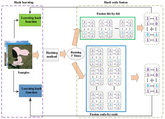
Figure 1: Flowchart of the proposed FH method. The two branches represent two fusion strategies that are discussed below. The “hashing method” can be replaced by other hashing algorithms.

II Proposed Method

The proposed FH is a two-step framework that first optimizes binary codes utilizing hash code fusion, then estimates hash function parameters based on the optimized hash codes. Given an existing hashing method, the proposed FH provides self-improvement capabilities. A flowchart for the proposed FH framework is presented in Fig. 1. FH consists of hash code fusion and hash learning steps. In the hash code fusion step, we first run a given hashing method $T$ times to obtain $T$ hash matrices for all samples. We then fuse the $T$ hash matrices utilizing two different fusion strategies. In the hash learning step, we learn a simple linear hash function based on the fused hash codes for out-of-sample extension.

In the following subsections, we first present some notations for FH and then describe the hash fusion and learning steps.

II-A Problem Statement and Notation

Generally, a hash function can have a form based on a linear projection, kernel, spherical function, neural network, etc. However, the linear function (or its variations, such as kernel and bilinear functions) is one of the most popular hash function forms because it is very efficient and easily optimized. Additionally, nearly all methods utilizing a linear hash function can be extended to kernelized hash functions [13]. Therefore, the theoretical analysis and hash learning methods proposed in this paper are largely based on linear hash functions.

In this paper, boldface lowercase letters, such as $\bf{h}$, denote vectors and boldface uppercase letters, such as $\bf{P}$, denote matrices. Furthermore, ${\rm{||}}{\bf{P}}||$ and ${{\bf{P}}^{T}}$ are utilized to denote the $\ell_{2}$-norm and transpose of a matrix $\bf{P}$, respectively. Boldface ${\bf{1}}$ denotes a vector where all elements are one. A few additional notations utilized in the proposed FH method are listed in Table I.

TABLE I: Notations

Notation	Description
$N$	number of samples
$L$	length of hash code
$T$	run times for a given hashing method
$H_{A}$	a given hashing method
${\bf{b}}_{i}$	the $i_{th}$-row of the hash matrix
${\bf{B}}_{i}$	hash matrix obtained from the $i_{th}$ run of hashing method $H_{A}$
$\bf{B}$	final hash matrix
$\bf{X}$	original feature matrix of size $L\times N$
$\bf{P}$	projection matrix between the hash matrix and feature matrix

II-B Hash Code Fusion

As discussed above, given a hashing method, we execute $T$ times to get $T$ hash codes $\{{{\bf{B}}_{i}\}_{i=1}^{T}}$ for use as a training set. Next, we fuse these $T$ hash codes into a final hash code ${\bf{B}}$ for use as a training sample. The motivation for hash code fusion is twofold. First, more accurate and stable codes can be obtained through hash code fusion. Second, synergy and relationships between different hash codes can be exploited through hash fusion. In this paper, we propose two fusion strategies. To describe these strategies, we first present some definitions and theorems, then outline the specific processes for the two fusion strategies.

It is known that learning-based hashing attempts to preserve the similarity relationships between samples in the original space based on Hamming distance. Therefore, different objective functions have been designed based on similarity preservation. In such optimization problems, there is a trivial solution in which all the hash codes of the samples are same (i.e., ${{\bf{b}}_{1}}={{\bf{b}}_{2}}=\cdots={{\bf{b}}_{N}}$). To avoid this solution, the code balance condition was introduced in [13]. It states that the number of data items mapped to each hash code must be the same. Bit balance and bit uncorrelation are utilized to approximate the code balance condition. Bit balance means that each bit has an approximately 50% chance of being $+1$ or $-1$. Bit uncorrelation means that different bits are uncorrelated. These two conditions are formulated as

$${\bf{B1}}=0,{\kern 1.0pt}{\kern 1.0pt}{\kern 1.0pt}{\kern 1.0pt}{\kern 1.0pt}{\kern 1.0pt}{\kern 1.0pt}{\kern 1.0pt}{\kern 1.0pt}{\kern 1.0pt}{\kern 1.0pt}{\bf{B}}{{\bf{B}}^{T}}=N{\bf{I}},$$ (2)

where $\bf{1}$ is an $N$-dimensional all-ones vector and $\bf{I}$ is an identity matrix of size $N$.

The property of code balance has proved to be very significant for hashing  [14]  [15]. In this study, to evaluate balance, we propose a definition called balance degree.

Balance degree: Given a hash matrix ${\bf{B}}\in{{\bf{R}}^{L\times N}}$, the balance degree of the $i_{th}$ bit for the samples is defined as the absolute value of the sum of the $i_{th}$ row in the hash matrix. For example, if the vector $\{-1,{\kern 1.0pt}{\kern 1.0pt}1,{\kern 1.0pt}{\kern 1.0pt}1,{\kern 1.0pt}{\kern 1.0pt}1\}$ is the $i_{th}$-row of the hash matrix, then the balance degree of the $i_{th}$ bit for the samples is $|-1+1+1+1|=2$. A smaller balance degree indicates better code balance.

We now present two theorems and their corresponding proofs, which are utilized in the proposed fusion strategies.

Theorem 1. Given a hash matrix ${\bf{B}}\in{{\bf{R}}^{L\times N}}$, duplicate rows can be removed from the hash matrix because they have no influence on the preservation of semantics.

Proof: Assume there are two hash matrices ${\bf{B}}=[\textbf{b}_{1};\textbf{b}_{2};...;\textbf{b}_{L}]$ and ${\bf{B^{\prime}}}=[\textbf{b}_{1};\textbf{b}_{2};...;\textbf{b}_{L};\textbf{b}_{L}]$. Compared to $\bf{B}$, there is one duplicate row in $\bf{B^{\prime}}$. One can see that ${\bf{B}}^{T}{\bf{B}}={\bf{B^{\prime}}}^{T}{\bf{B^{\prime}}}+const$. That is to say, after adding a duplicate row to the hash matrix $\bf{B}$, the similarity between different hash codes remained unchanged. Therefore, there is no influence on the Hamming distance between different samples. In other words, duplicate hash bits can also be removed without any influence on the preservation of semantics.

Furthermore, assume $\bf{P}$ is a projection between an original feature and hash code. The loss for hash learning can be simply calculated as follows:

$$\min\limits_{{\bf{P}}}\left\|{\bf{B}}-{\bf{P}}^{T}{\bf{X}}\right\|^{2}+\lambda\left\|{\bf{P}}\right\|^{2}\quad{s.t.}\quad{\bf{B}}\in\left\{-1,1\right\}^{L\times n}.$$ (3)

Set the derivative of the objective function in Equation (3) w.r.t ${\bf{P}}$ to 0. Then,

$${\bf{XX}}^{T}{\bf{P}}+\lambda{\bf{P}}-{\bf{X}}{\bf{B}}^{T}=0.$$ (4)

The closed-form solution of ${\bf{P}}$ can be derived as

$${\bf{P}}=({\bf{XX}}^{T}+\lambda{\bf{I}})^{-1}{\bf{X}}{\bf{B}}^{T}.$$ (5)

For hash matrices $\bf{B}$ and $\bf{B^{\prime}}$, we have ${\bf{P}_{B}}=({\bf{XX}}^{T}+\lambda{\bf{I}})^{-1}{\bf{X}}{\bf{B}}^{T}$ and ${\bf{P^{\prime}}_{B^{\prime}}}=({\bf{XX}}^{T}+\lambda{\bf{I}})^{-1}{\bf{X}}{\bf{B^{\prime}}}^{T}$, respectively. We define ${\bf{Q}}=({\bf{XX}}^{T}+\lambda{\bf{I}})^{-1}{\bf{X}}$. Then, we have ${\bf{P}_{B}}={\bf{Q}}{\bf{B}}^{T}$ and ${\bf{P^{\prime}}_{B^{\prime}}}={\bf{Q}}{\bf{B^{\prime}}}^{T}=[{\bf{P}_{A}};{\bf{Q}}\,\textbf{b}_{L}]$. Finally,

$$\begin{split}\left\|{\bf{B^{\prime}}}-{\bf{P^{\prime}}_{B^{\prime}}}^{T}{\bf{X}}\right\|^{2}&=\left\|{\bf{B}}-{\bf{B}}{\bf{Q}}^{T}{\bf{X}}\right\|^{2}+\left\|\textbf{b}_{L}-\textbf{b}_{L}{\bf{Q}}^{T}{\bf{X}}\right\|^{2}\\ &=({\bf{I}}+const)\left\|{\bf{B}}-{\bf{B}}{\bf{Q}}^{T}{\bf{X}}\right\|^{2}\\ &=({\bf{I}}+const)\left\|{\bf{B}}-{\bf{P}_{B}}^{T}{\bf{X}}\right\|^{2}.\end{split}$$ (6)

One can see that the fitting error is unchanged.

In conclusion, there is no influence on semantic preservation when duplicate rows are removed from the hash matrix.

Theorem 2. Given a hash matrix ${\bf{B}}\in{{\bf{R}}^{L\times N}}$, the hash bit rows of $\bf{B}$ can be out of order because ordering has no influence on semantic preservation.

Proof: For the hash matrix ${\bf{B}}=[\textbf{b}_{1};\textbf{b}_{2};...;\textbf{b}_{L}]$, ${\bf{B^{\prime}}}$ is a hash matrix whose hash bit rows are a random permutation of $\bf{B}$. One can see that ${\bf{B}}^{T}{\bf{B}}={\bf{B^{\prime}}}^{T}{\bf{B^{\prime}}}$. Therefore, the semantics can be preserved, even if the hash bits are out of order.

Furthermore, according to Eqs. (3) and (4), for hash matrices $\bf{B}$ and $\bf{B^{\prime}}$, we have ${\bf{P}_{B}}=({\bf{XX}}^{T}+\lambda{\bf{I}})^{-1}{\bf{X}}{\bf{B}}^{T}$ and ${\bf{P^{\prime}}_{B^{\prime}}}=({\bf{XX}}^{T}+\lambda{\bf{I}})^{-1}{\bf{X}}{\bf{B^{\prime}}}^{T}$, respectively. One can see that $\left\|{\bf{P}_{B}}\right\|^{2}=\left\|{\bf{P^{\prime}}_{B^{\prime}}}\right\|^{2}$. We define ${\bf{Q}}=({\bf{XX}}^{T}+\lambda{\bf{I}})^{-1}{\bf{X}}$. Then, we have

$$\begin{split}\left\|{\bf{B}}-{\bf{P}_{B}}^{T}{\bf{X}}\right\|^{2}&=\left\|{\bf{B}}-{\bf{B}}{\bf{Q}}^{T}{\bf{X}}\right\|^{2}\\ &=\left\|{\bf{B}}({\bf{I}}-{\bf{Q}}^{T}{\bf{X}})\right\|^{2}\\ &=\left\|{\bf{B}}{\bf{W}}\right\|^{2}\\ &=trace({\bf{W}}^{T}{\bf{B}}^{T}{\bf{B}}{\bf{W}})\\ &=trace({\bf{B}}^{T}{\bf{B}}{\bf{W}}{\bf{W}}^{T}),\end{split}$$ (7)

where ${\bf{W}}={\bf{I}}-{\bf{Q}}^{T}{\bf{X}}$. Therefore, we have $\left\|{\bf{B}}-{\bf{P}_{B}}^{T}{\bf{X}}\right\|^{2}=\left\|{\bf{B^{\prime}}}-{\bf{P^{\prime}}_{B^{\prime}}}^{T}{\bf{X}}\right\|^{2}$ because ${\bf{B}}^{T}{\bf{B}}={\bf{B^{\prime}}}^{T}{\bf{B^{\prime}}}$. That is to say, $\left\|{\bf{B}}-{\bf{P}_{B}}^{T}{\bf{X}}\right\|^{2}+\lambda\left\|{\bf{P}_{B}}\right\|^{2}=\left\|{\bf{B^{\prime}}}-{\bf{P^{\prime}}_{B^{\prime}}}^{T}{\bf{X}}\right\|^{2}+\lambda\left\|{\bf{P^{\prime}}_{B^{\prime}}}\right\|^{2}$. One can see that the fitting error remains unchanged.

In conclusion, there is no influence on semantic preservation when the hash bit rows of $\bf{B}$ are out of order.

We now propose two novel fusion strategies to obtain more accurate and stable hash codes for training samples.

II-B1 Bit-by-bit fusion

Given a hashing method $H_{A}$, after executing it $T$ times in the training set, we obtain $T$ different hash matrices $\{{{\bf{B}}_{i}}\}_{i=1}^{T}\in{{\bf{R}}^{L\times N}}$, where ${{\bf{B}}_{i}}=({\bf{b}}_{l}^{i})_{l=1}^{L}$ and ${\bf{b}}_{l}^{i}\in{{\bf{R}}^{1\times N}}$. One can see that ${\bf{b}}_{l}^{i}$ is the $l_{th}$-row of hash matrix ${\bf{B}}_{i}$.

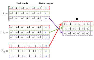
Figure 2: Illustration of the bit-by-bit fusion strategy. The first row of ${\bf{B}}$ comes from the first row of ${\bf{B}}_{i}$, whose balance degree is the minimum one among the corresponding rows in all hash matrices. The second and third rows are similarly obtained.

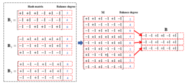
Figure 3: Illustration of the code-by-code fusion strategy. We concatenate three hash matrices to obtain the matrix $\bf{M}$, then select the three rows with the minimum balance degrees to construct the matrix $\bf{B}$.

The goal of hash fusion is to obtain an accurate and stable hash matrix $\bf{B}$ for all training samples from the $T$ hash matrices $\{{{\bf{B}}_{i}}\}_{i=1}^{T}$. Here, we propose a bit-by-bit fusion strategy based on the code balance condition. For the $l_{th}$-bit (i.e., the $l_{th}$-row in $\bf{B}$) of all training samples, we first compute the balance degrees of the $l_{th}$-bit in all hash matrices $\{{{\bf{B}}_{i}}\}_{i=1}^{T}$, then select the row whose balance degree is the smallest among all hash matrices $\{{{\bf{B}}_{i}}\}_{i=1}^{T}$, meaning we find the most balanced bit row among all hash matrices. If there are two or more rows with the same minimum balance degree, we empirically select the row in the first hash matrix. It should be noted that this phenomenon is rarely seen when the number of samples is large. We repeat this process for all $L$ rows to obtain a final hash matrix $\bf{B}$. Additionally, if there are duplicate rows in hash matrix ${\bf{B}}$, they are removed according to Theorem 1 to obtain more compact hash codes.

To demonstrate the bit-by-bit strategy, we presented an example in Fig. 2, where $T$=3, $L$=3, and $N$=6. For each row in the three hash matrices $\{{\bf{B}}_{i}\}_{i=1}^{3}$, we compute a balance degree. The row with the smallest balance degree among the three hash matrices $\{{\bf{B}}_{i}\}_{i=1}^{3}$ is selected as a row of $\bf{B}$.

II-B2 Code-by-code fusion

In this strategy, given $T$ hash matrices $\{{{\bf{B}}_{i}}\}_{i=1}^{T}$, in contrast to bit-by-bit fusion, we randomly concatenate all hash matrices in the column direction. According to Theorem 2, random ordering has no impact on semantic preservation and we obtain a new matrix ${\bf{M}}\in{{\bf{R}}^{TL\times N}}$. If we wish to obtain a hash code of length $L$, we then select the first $L$ rows from matrix ${\bf{M}}$ with minimum balance degrees to construct the final hash matrix $\bf{B}$. If there are duplicate rows in hash matrix ${\bf{B}}$, they are removed according to Theorem 1 to obtain more compact hash codes.

We present an example in Fig. 3, where $T$=3, $L$=3, and $N$=6. In this example, we first concatenate the hash matrices ${\bf{B}}_{1}$, ${\bf{B}}_{2}$, and ${\bf{B}}_{3}$ in the column direction, then select the first three rows with minimum balance degrees to construct the final hash matrix $\bf{B}$.

II-B3 Discussion

To adequately describe the motivation for hash fusion strategies, we can consider a hash bit as a binary feature of the training samples, where a more balanced bit represents a better feature. Therefore, the goal of the two proposed fusion strategies is to replace bad binary features with good binary features. Additionally, according to Theorem 2, we can neglect the order of the hash bits. Therefore, good binary features (which have minimum balance degrees) can be sampled more than once, which is another motivation for the code-by-code fusion strategy.

II-C Hash Learning

After obtaining a desirable hash matrix of training samples, we then learn a hash function for out-of-sample inputs. Generally, any type of hash function, such as a kernel, spherical function, neural network, or nonparametric function, can be utilized in this step. However, we utilized a linear hash function in this study. A simple form of the relevant optimization problem can be written as follows:

$$\min\limits_{{\bf{P}}}\left\|{\bf{B}}-{\bf{P}}^{T}{\bf{X}}\right\|^{2}+\lambda\left\|{\bf{P}}\right\|^{2}.$$ (8)

The matrix $\bf{B}$ is obtained following hash code fusion and the solution of $\bf{P}$ can be easily obtained by utilizing Eqs. (4) and (5). Based on the learned projection $\bf{P}$, we can obtain hash codes for out-of-sample inputs by utilizing a sign function.

In summary, the proposed FH is presented in Algorithm 1.

Algorithm 1 Fusion Hashing (FH)

1:Training sets ${\bf{X}}$; hash code length $L$; given hashing algorithm $H_{A}$; number of iterations $T$.

2:Initialize ${\bf{P}}$ as a random matrix.

3:Execute hashing algorithm $H_{A}$ $T$ times to get $T$ hash matrices.

4:Fuse $T$ hash matrices to get a final hash matrix ${\bf{B}}$ utilizing bit-by-bit fusion or code-by-code fusion.

5:Utilize Eq. (5) to solve ${\bf{P}}$.

6:Projection matrix ${\bf{P}}$.

II-D Time complexity analysis

We assume that the time complexity for a given hash algorithm $H_{A}$ is $C$. Then, the time complexity for generating $T$ hash codes is $T\cdot C$. Additionally, the time complexity for solving the linear projection ${\bf{P}}$ is $O(NdL+Nd^{2})$, where $d$ is the dimension of the input features. For hash fusion, the time complexity depends on the fusion strategy. In the balance degree sorting process, the time complexity is typically no greater than $O(TLlgL)$. In the process of balance degree computation, the time complexity is $O(NTL)$. Therefore, the time complexity for FH during training is $O(NdL+Nd^{2}+TLlgL+NTL)+T\cdot C$. Because $L$ and $T$ are much smaller than $d$ and $N$, the time complexity for FH during training can be rewritten as $O(Nd^{2})+T\cdot C$. In general, compared to the time complexity of the hash algorithm $H_{A}$, the time complexity for learning the linear projection ${\bf{P}}$ is negligible. Therefore, the proposed FH method is only $T$ times as complex as the original hashing method, but achieves superior precision. Additionally, the value $T$ is always small because we found that a small $T$ value is acceptable based on our experiments. Precision only increases very slowly with an increase in $T$. Therefore, the proposed framework does not require significant extra expenditures in terms of time and space to achieve superior precision.

III Experiments

In this section, we present our experimental settings and results. Three image datasets were utilized to evaluate the performance of the proposed method. Extensive experiments were conducted to evaluate the proposed framework. Our experiments were conducted on a computer with an Intel(R) Core(TM) i7-4790 CPU and 16 GB of RAM. The hyperparameter settings employed are listed in the experimental settings section.

III-A Experimental Settings

TABLE II: Performance in terms of MAP score with data independent method.

Method	CIFAR-10			MS-COCO			NUS-WIDE
	24 bits​	48 bits​	64 bits​	24 bits​	48 bits​	64 bits​	24 bits​	48 bits​	64 bits​
LSH	0.2604	0.2942	0.3101	0.6093	0.7121	0.7145	0.4095	0.5968	0.5934
LSH	0.2600	0.2901	0.3027	0.6338	0.6715	0.6558	0.5407	0.6109	0.5903
LSH	0.2704	0.2908	0.2898	0.6404	0.6548	0.7051	0.4754	0.5814	0.5969
FHBB	0.3046	0.3441	0.3656	0.7224	0.7629	0.7576	0.5790	0.7027	0.6853
FHCC	0.3041	0.3450	0.3753	0.7260	0.7677	0.7712	0.5946	0.7096	0.6831

TABLE III: Performance in terms of MAP score with unsupervised methods.

Method	CIFAR-10			MS-COCO			NUS-WIDE
	24 bits​	48 bits​	64 bits​	24 bits​	48 bits​	64 bits​	24 bits​	48 bits​	64 bits​
PCA-ITQ	0.3418	0.3502	0.3547	0.6273	0.6967	0.7166	0.4048	0.6169	0.6390
PCA-ITQ	0.3429	0.3539	0.3555	0.6276	0.6917	0.7154	0.4054	0.6171	0.6471
PCA-ITQ	0.3354	0.3461	0.3521	0.6330	0.6907	0.7152	0.4057	0.6109	0.6382
FHBB	0.3172	0.3570	0.3725	0.6395	0.6824	0.7095	0.3846	0.6190	0.6532
FHCC	0.3296	0.3641	0.3747	0.6665	0.6842	0.7062	0.3847	0.6196	0.6552
PCA-RR	0.2987	0.3114	0.3222	0.6596	0.6781	0.6970	0.4596	0.5941	0.5961
PCA-RR	0.2787	0.3221	0.3285	0.6205	0.6865	0.6863	0.5001	0.6059	0.5573
PCA-RR	0.3017	0.3204	0.3235	0.5561	0.7194	0.7397	0.4960	0.5990	0.6238
FHBB	0.3072	0.3456	0.3691	0.7223	0.7692	0.7783	0.6013	0.6886	0.7018
FHCC	0.3312	0.3483	0.3776	0.7237	0.7754	0.7794	0.5981	0.6983	0.7037
SH	0.2908	0.2961	0.2992	0.6616	0.6501	0.6659	0.6070	0.5986	0.5934
SH	0.2908	0.2961	0.2992	0.6616	0.6501	0.6659	0.6070	0.5986	0.5934
SH	0.2908	0.2961	0.2992	0.6616	0.6501	0.6659	0.6070	0.5986	0.5934
FHBB	0.3191	0.3323	0.3430	0.7130	0.7173	0.7355	0.6501	0.6690	0.6661
FHCC	0.2689	0.2665	0.2760	0.5536	0.6051	0.6343	0.5210	0.5521	0.6084

TABLE IV: Performance in terms of MAP score with supervised methods.

Method	CIFAR-10			MS-COCO			NUS-WIDE
	24 bits​	48 bits​	64 bits​	24 bits​	48 bits​	64 bits​	24 bits​	48 bits​	64 bits​
SDH	0.2333	0.4622	0.4007	0.8026	0.8413	0.5948	0.6837	0.7045	0.7036
SDH	0.2236	0.5346	0.4797	0.6280	0.7204	0.8452	0.6888	0.7611	0.6844
SDH	0.2640	0.4322	0.3089	0.8019	0.5156	0.8219	0.5004	0.6683	0.6926
FHBB	0.2013	0.5004	0.3618	0.8101	0.6355	0.7629	0.6303	0.7410	0.7367
FHCC	0.2124	0.4090	0.2932	0.8120	0.6678	0.7836	0.6648	0.7528	0.7389
COSDISH	0.4566	0.5034	0.5269	0.5082	0.5900	0.6563	0.3633	0.4192	0.4007
COSDISH	0.4795	0.5034	0.5143	0.5850	0.6890	0.6505	0.4351	0.4830	0.4531
COSDISH	0.4817	0.5268	0.5184	0.4967	0.6006	0.6078	0.4452	0.4555	0.4894
FHBB	0.5559	0.6112	0.6021	0.6011	0.7657	0.7399	0.5181	0.5826	0.5458
FHCC	0.5827	0.6310	0.6255	0.6011	0.7646	0.7485	0.5181	0.5845	0.5455
FSDH	0.6444	0.6798	0.6838	0.8122	0.8246	0.8209	0.7750	0.7756	0.7866
FSDH	0.6443	0.6687	0.6872	0.7810	0.8232	0.8371	0.7750	0.7865	0.7878
FSDH	0.6324	0.7006	0.7019	0.8151	0.8218	0.8234	0.7705	0.7798	0.7873
FHBB	0.6682	0.6914	0.7004	0.8296	0.8394	0.8512	0.7713	0.7876	0.7895
FHCC	0.6657	0.7006	0.7019	0.8367	0.8426	0.8536	0.7840	0.7913	0.7942

III-A1 Datasets

We utilized three different image datasets, namely CIFAR-10 [16], MS-COCO [17], and NUS-WIDE [18], in our experiments. These datasets are widely used in image retrieval studies. CIFAR-10 is a single-label dataset containing 60,000 images that belong to 10 classes, with 6,000 images per class. We randomly selected 5,000 and 1,000 images (100 images per class) from the dataset as our training and testing sets, respectively.

The MS-COCO dataset is a multi-label dataset containing 82,783 images that belong to 91 categories. For the training image set, images with no category information were discarded and 82,081 remained. For the MS-COCO dataset, two images were defined as a similar pair if they shared at least one common label. We randomly selected 10,000 and 5,000 images from the dataset as our training and testing sets, respectively.

The NUS-WIDE dataset contains 269,648 web images associated with 1,000 tags. In this multi-label dataset, each image may be annotated with multiple labels. We only selected 195,834 images belonging to the 21 most frequent concepts. For the NUS-WIDE dataset, two images were defined as a similar pair if they shared at least one common label. We randomly selected 10,500 (500 from each concept) and 2,100 (100 from each concept) images from the dataset as our training and testing sets, respectively.

In this study, we employed a convolutional neural network (CNN) model called the CNN-F model [19] to perform feature learning. The CNN-F model has also been applied in deep pairwise-supervised hashing [20]and asymmetric deep supervised hashing [21] for feature learning. The CNN-F model contains five convolutional layers and three fully-connected layers. Their details are provided in [19]. It should be noted that the FH framework is sufficiently general to allow other deep neural networks to replace the CNN-F model for feature learning. In this study, we only employed the CNN-F model for illustrative purposes. Additionally, a radial basis function was utilized to reduce the number of parameters. The 4,096 deep features extracted by the CNN-F model were mapped to 1,000 features.

III-A2 Evaluation Metrics

To evaluate the proposed method, we utilized an evaluation metric known as mean average precision (MAP), which is used widely in image retrieval evaluation. MAP is the mean of the average precision values obtained for the top retrieved samples.

$$\textup{MAP}=\frac{1}{Q}\sum_{r=1}^{Q}\textup{AP}(i),$$ (9)

where $Q$ is the number of query images and $\textup{AP}(i)$ is the AP of the $i_{th}$ instance. AP is defined as

$$\textup{AP}=\frac{1}{R}\sum_{r=1}^{G}precision(r)\sigma(r),$$ (10)

where $R$ is the number of relevant instances in the retrieved $G$ samples. Here, $\sigma(r)$ = 1 if the $r_{th}$ instance is relevant to the query. Otherwise, $\sigma(r)$ = 0.

III-B Experimental Results and Analysis

We applied the proposed FH framework to the following methods: LSH  [22], spectral hashing (SH)  [23], principle component analysis (PCA)-iterative quantization (PCA-ITQ)  [24], PCA-random rotation  [24], supervised discrete hashing (SDH)  [3], column sampling based discrete supervised hashing  [1], and fast supervised discrete hashing (FSDH)  [25]. LSH is a data-independent method. SH, PCA-ITQ, and PCA-RR are unsupervised hashing methods. All the other methods are supervised hashing methods. All of the hyperparameters were initialized as suggested in the original publications. The proposed FH is a data-dependent framework. However, the proposed FH can be applied to data-independent method such as LSH.

The proposed FH with the bit-by-bit strategy is denoted FHBB, whereas FH with the code-by-code strategy is denoted FHCC. We executed the original methods three times each. In other words, we set $T=3$.

Table II lists the MAP scores of the data-independent LSH method with hash lengths ranging from 24–64 bits. One can see that the performance was improved by applying the proposed FH to LSH on all three benchmark datasets. FHBB and FHCC resulted in similar performance and both achieved 4%$-$12% MAP score improvements for the three benchmark datasets.

Table III lists the MAP scores of the unsupervised methods with hash lengths ranging from 24–64 bits. One can see that the performances of the unsupervised methods were also improved by the proposed FHBB and FHCC in most cases. However, the proposed FHCC could not improve the performance of the SH method. One possible reason is that the performance of this method is so stable that the MAP does not change based on the number of executions. However, FHBB still improved the MAP performance of SH. This indicates that the proposed FHBB and FHCC can be applied in different scenarios with different results. We plan to investigate to best scenarios for each strategy in a future study.

Table IV lists the MAP scores of the supervised methods with hash lengths ranging from 24–64 bits. We can see similar results to those listed in Table III. When applying FHBB and FHCC, superior performance was achieved in most cases. It is worth mentioning that when applying the proposed framework to the SDH method, the performance was not always improved. The main reason for this is that SDH is very unstable, which leads to widely varying MAP performances for different executions. Then, a hash code with a bad MAP has a negative effect on hash code fusion. Compared to SDH, the FSDH method, which is a stable version of SDH, saw significant improvements with the application of FHBB and FHCC.

Fig. 4 presents the precision results for the three benchmark datasets with hash lengths ranging from 12–128 bits, where $method-abbreviation_{i}$ represents the $i_{th}$ running for the method, such as $LSH_{1}$. Five methods were selected for tested and we executed the original methods three times. One can see that the proposed FHBB and FHCC almost produce superior precision, except for FHBB with the SH method.

Fig. 5 and Fig. 6 show the Precision@ 5000 on three benchmark datasets with the hash length ranging from 24–128 bits and the number of running times ranging from 2–6 bits by using the fusion strategy FHBB and FHCC, respectively. Five methods are selected limited by the space. It can be seen that the precisions of hashing methods are improved by using the proposed fusion strategies with the number of running times and hash bit being bigger. However, we can see that the precision increases slowly with bigger number of running times, which indicates that the proposed framework does not need too much extra expenditure in term of time and space to get superior precision.

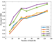
(a) Based on CIFAR-10

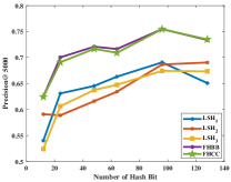
(b) Based on MS-COCO

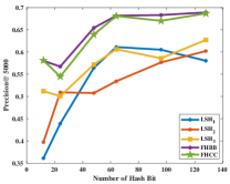
(c) Based on NUS-WIDE

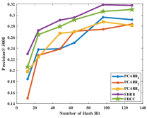
(d) Based on CIFAR-10

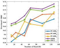
(e) Based on MS-COCO

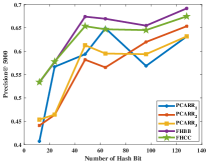
(f) Based on NUS-WIDE

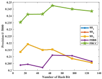
(g) Based on CIFAR-10

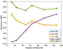
(h) Based on MS-COCO

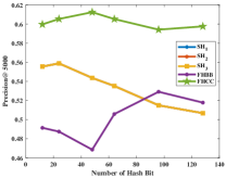
(i) Based on NUS-WIDE

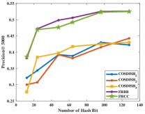
(j) Based on CIFAR-10

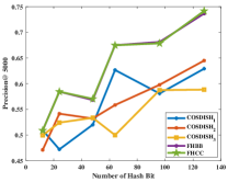
(k) Based on MS-COCO

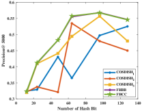
(l) Based on NUS-WIDE

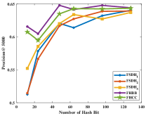
(m) Based on CIFAR-10

(n) Based on MS-COCO

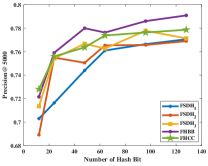
(o) Based on NUS-WIDE

Figure 4: Precision@ 5000 with different number of hash bit based on three benchmark datasets.

(a) Based on CIFAR-10

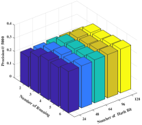
(b) Based on MS-COCO

(c) Based on NUS-WIDE

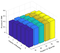
(d) Based on CIFAR-10

(e) Based on MS-COCO

(f) Based on NUS-WIDE

(g) Based on CIFAR-10

(h) Based on MS-COCO

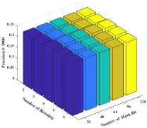
(i) Based on NUS-WIDE

(j) Based on CIFAR-10

(k) Based on MS-COCO

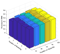
(l) Based on NUS-WIDE

(m) Based on CIFAR-10

(n) Based on MS-COCO

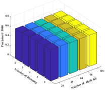
(o) Based on NUS-WIDE

Figure 5: Precision@ 5000 with different setting of number of hash bit and running times based on three benchmark datasets using FHBB. (From top to bottom: LSH, PCARR, SH, COSDISH, FSDH).

(a) Based on CIFAR-10

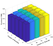
(b) Based on MS-COCO

(c) Based on NUS-WIDE

(d) Based on CIFAR-10

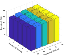
(e) Based on MS-COCO

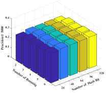
(f) Based on NUS-WIDE

(g) Based on CIFAR-10

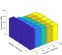
(h) Based on MS-COCO

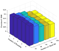
(i) Based on NUS-WIDE

(j) Based on CIFAR-10

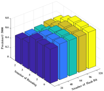
(k) Based on MS-COCO

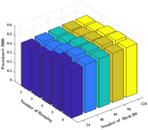
(l) Based on NUS-WIDE

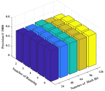
(m) Based on CIFAR-10

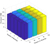
(n) Based on MS-COCO

(o) Based on NUS-WIDE

Figure 6: Precision@ 5000 with different setting of number of hash bit and running times based on three benchmark datasets using FBCC. (From top to bottom: LSH, PCARR, SH, COSDISH, FSDH).

IV Conclusion

In this study, we proposed a general framework called FH to facilitate the self-improvement of various hashing methods. Generally, the proposed framework can be applied to existing hashing methods without adding new constraint terms. In the proposed framework, we implemented two fusion strategies to obtain more accurate and stable hash codes from a given original hashing method. We then learn a simple linear projection for out-of-sample inputs. Experiments conducted on three benchmark datasets demonstrated the superior performance of the proposed framework.

References

- [1] W.-C. Kang, W.-J. Li, and Z.-H. Zhou, “Column sampling based discrete supervised hashing.” in AAAI, 2016, pp. 1230–1236.
- [2] Z. Yu, F. Wu, Y. Yang, Q. Tian, J. Luo, and Y. Zhuang, “Discriminative coupled dictionary hashing for fast cross-media retrieval,” in Proceedings of the 37th international ACM SIGIR conference on Research & development in information retrieval. ACM, 2014, pp. 395–404.
- [3] F. Shen, C. Shen, W. Liu, and H. Tao Shen, “Supervised discrete hashing,” in Proceedings of the IEEE Conference on Computer Vision and Pattern Recognition, 2015, pp. 37–45.
- [4] Y. Weiss, A. Torralba, and R. Fergus, “Spectral hashing,” in International Conference on Neural Information Processing Systems, 2008, pp. 1753–1760.
- [5] M. Raginsky and S. Lazebnik, “Locality-sensitive binary codes from shift-invariant kernels,” in Advances in neural information processing systems, 2009, pp. 1509–1517.
- [6] A. Dasgupta, R. Kumar, and T. Sarlós, “Fast locality-sensitive hashing,” in Proceedings of the 17th ACM SIGKDD international conference on Knowledge discovery and data mining. ACM, 2011, pp. 1073–1081.
- [7] J. Ji, J. Li, S. Yan, Q. Tian, and B. Zhang, “Min-max hash for jaccard similarity,” in IEEE International Conference on Data Mining, 2014, pp. 301–309.
- [8] J. Wang, S. Kumar, and S.-F. Chang, “Semi-supervised hashing for large-scale search,” IEEE Transactions on Pattern Analysis and Machine Intelligence, vol. 34, no. 12, pp. 2393–2406, 2012.
- [9] W. Liu, J. Wang, R. Ji, and Y. G. Jiang, “Supervised hashing with kernels,” in Computer Vision and Pattern Recognition, 2012, pp. 2074–2081.
- [10] G. Lin, C. Shen, and A. van den Hengel, “Supervised hashing using graph cuts and boosted decision trees,” IEEE transactions on pattern analysis and machine intelligence, vol. 37, no. 11, pp. 2317–2331, 2015.
- [11] Q. Wang, Z. Zhang, and L. Si, “Ranking preserving hashing for fast similarity search.” in IJCAI, 2015, pp. 3911–3917.
- [12] J. Gui, T. Liu, Z. Sun, D. Tao, and T. Tan, “Supervised discrete hashing with relaxation,” IEEE transactions on neural networks and learning systems, 2016.
- [13] J. Wang, T. Zhang, J. Song, N. Sebe, and H. T. Shen, “A survey on learning to hash,” arXiv preprint arXiv:1606.00185, 2016.
- [14] F. Shen, X. Gao, L. Liu, Y. Yang, and H. T. Shen, “Deep asymmetric pairwise hashing,” in Proceedings of the 2017 ACM on Multimedia Conference. ACM, 2017, pp. 1522–1530.
- [15] Q. Y. Jiang and W. J. Li, “Deep cross-modal hashing,” in arxiv, 2016.
- [16] A. Krizhevsky and G. Hinton, “Learning multiple layers of features from tiny images,” Citeseer, Tech. Rep., 2009.
- [17] T.-Y. Lin, M. Maire, S. Belongie, J. Hays, P. Perona, D. Ramanan, P. Dollár, and C. L. Zitnick, “Microsoft coco: Common objects in context,” in European conference on computer vision. Springer, 2014, pp. 740–755.
- [18] T.-S. Chua, J. Tang, R. Hong, H. Li, Z. Luo, and Y. Zheng, “Nus-wide: a real-world web image database from national university of singapore,” in Proceedings of the ACM international conference on image and video retrieval. ACM, 2009, p. 48.
- [19] K. Chatfield, K. Simonyan, A. Vedaldi, and A. Zisserman, “Return of the devil in the details: Delving deep into convolutional nets,” arXiv preprint arXiv:1405.3531, 2014.
- [20] W.-J. Li, S. Wang, and W.-C. Kang, “Feature learning based deep supervised hashing with pairwise labels,” In IJCAI, 2017.
- [21] Q.-Y. Jiang and W.-J. Li, “Asymmetric deep supervised hashing,” Proceedings of the 32nd AAAI Conference on Artificial Intelligence (AAAI), 2018, 2018.
- [22] A. Gionis, P. Indyk, and R. Motwani, “Similarity search in high dimensions via hashing,” International Conference on Very Large Data Bases, vol. 8, no. 2, pp. 518–529, 1999.
- [23] Y. Weiss, A. Torralba, and R. Fergus, “Spectral hashing,” in Advances in neural information processing systems, 2009, pp. 1753–1760.
- [24] Y. Gong and S. Lazebnik, “Iterative quantization: A procrustean approach to learning binary codes,” in IEEE Conference on Computer Vision and Pattern Recognition, 2011, pp. 817–824.
- [25] J. Gui, T. Liu, Z. Sun, D. Tao, and T. Tan, “Fast supervised discrete hashing,” IEEE transactions on pattern analysis and machine intelligence, vol. 40, no. 2, pp. 490–496, 2018.