Topological defects in helical magnets

Abstract

Helical magnets which violated space inversion symmetry have rather peculiar topological defects. In isotropic helical magnets with exchange and Dzyaloshinskii-Moriya interactions there are only three types of linear defects: $\pm\pi$ and $2\pi$-disclinations. Weak crystal anysotropy suppresses linear defects on large scale. Instead planar defects appear: domain walls that separate domains with different preferential directions of helical wave vectors. The appearance of such domain walls in the bulk helical magnets and some of their properties were predicted in the work Li 2012 . In a recent work by an international team of experimenters and theorists Schoenherr 2018 the existence of new types of domain walls on crystal faces of helical magnet FeGe was discovered. They have many features predicted by theory Li 2012 , but display also unexpected properties, one of them is the possibility of arbitrary angle between helical wave vectors. Depending on this angle the domain walls observed in Schoenherr 2018 can be divided in two classes: smooth and zig-zag. This article contains a mini-review of the existing theory and experiment. It also contains new results that explain why in a system with continuos orientation of helical wave vectors domain walls are possible. We discuss why and at what conditions smooth and zig-zag domain walls appear, analyze spin textures associated with helical domain walls and find the dependence of their width on angle between helical wave vectors.

I Introduction

We are happy to congratulate Lev Pitaevskii on occasion of his Jubilee. We are amazed by the depth and brilliance of his scientific achievements that include such pearls as the Gross-Pitaevskii equation and the Theory of electromagnetic fluctuations in dispersive media. But not less surprising is his universalism, so rare in our time, and his irreproachable scientific integrity. These qualities together made him a unique person, able to continue the magnificient Landau-Lifshitz compendium of modern theoretical physics. The fact that it is still not simply alive after the death of both inital authors, but is an indispensable belonging of any private and institutional physical library, is the result of his tireless work. One of us (VP) has the privilege and pleasure to be in friendship with him starting from the end of 1950-th. He learned a lot from scientific discussions with Lev but not only that. Lev’s natural kindness and sincerity is an important part of life for all his friends. We wish him good health and high spirit.

In this article, written in his honour, we review theory and experiment on topological defects in helical magnets. Topological defects are among the most facscinating objects of condensed matter physics and quantum field theory Toulouse 1976 ; Volovik 1977 ; Chaikin 1995 ; Volovik 2003 ; Polyakov 1987 . They almost unavoidably appear in ordered phases, either as a result of initial conditions like cosmic strings Polyakov 1987 ; Volovik 2003 , or as equilibrium configurations like vortex lattices in type-II superconductors Abrikosov 1957 and superfluids Onsager 1949 ; Feynman 1955 . Defects counteract the emergent rigidity of the condensate and hence are fundamental both from the point of view of basic science as well as of practical applicationsHaasen 1971 ; Anderson 1984

Topological defects are different in systems with different symmetries and types of its violation in the ordered states. Some of them are well known, for example quantized vortices in quantum liquids Onsager 1949 ; Abrikosov 1957 or domain walls in magnets. Skyrmions Skyrme 1962 ; Belavin 1975 ; Abanov 1998 are more sophisticated but obtained a broad advertisement recently due to experiments in 2-dimensional magnets and nuclear matterBogdanov 1994 ; Muhlbauer 2009 ; Yu 2010 ; Kiselev 2011 ; Fert 2017 . Defects in superfluid helium 3 with its complex ordering are more exotic. Their description and literature can be found in the book by Volovik Volovik 1992 .

Topological defects in helical magnets are interesting not only as a subject of pure science, but also because they interact with electric current and thus may serve for transformation of magnetic signals into electric ones and back, that is a basic element of sensing, transfer and storing of information and energy.

In the year 2012 Fuxiang Li and the authors published an article on domain walls in helical magnets, in which we predicted rather unusual properties of these defects Li 2012 . Most of these predictions were confirmed in a fundamental experiments performed by the international team of experimenters and theorists in 2018 Schoenherr 2018 , but not all and some unexpected features appeared. In the following text we analyze these experiments and explain some of discrepancies between our theory and the experimental observations. Explanations of other facts require a further development of theory. The main reason of discrepancies is that Magnetic Force Microscope (MFM), used in these experiments, gives information on magnetic textures on crystal faces of samples, whereas our theory had in mind the bulk.

The content of the following article is as follows. In the second section we present a general analysis of the topological defects in isotropic helical magnets. In the third section we consider in more details domain walls in the bulk helical magnets. The fourth section is dedicated to helical domain walls at crystal faces. It contains a brief description of the experimental observations made in the work Schoenherr 2018 and modifications of the domain walls theory necessary in this situation. In this section we compare theory given in our article and in the cited publication by international group and experiment. In Conclusion we summarize new results of this article and discuss unsolved problems.

We conclude the introduction by a brief description of the interactions essential for helical magnets and the structure of helical ordering without defects. In this article we consider systems without inversion symmetry. The violation of this symmetry in helical magnets is associated with Dzyaloshinskii-Moriya interaction. Typical helical magnets with these properties are alloys MnSi Muhlbauer 2004 , FeGe Uchida 2008 , $\mathrm{Fe_{x}Co_{1-x}Si}$ Uchida 2006 . The Hamiltonian of spin system in these helical magnets in continuous approximation can be represented as follows:

$$\mathcal{H}=\!\int\!d^{3}x\left[\frac{J}{2}(\bm{\nabla}\bm{m})^{2}+g\bm{m}\left(\bm{\nabla}\times\bm{m}\right)+\frac{v}{4}\sum_{\alpha=1}^{3}m_{\alpha}^{4}\right].$$ (1)

Here we measured all lengths in units of the lattice parameter $a$. The first term in (1) represents the exchange interaction, the second is the Dzyaloshinskii-Moriya (DM) interaction and the third term is the crystal field energy corresponding to cubic anisotropy of the lattice. The dimensionless magnetization vector $\mathbf{m}$ in this approach has unit length. The hierarchy of interactions is $J\gg g\gg v$.

In the absence of crystal field the energy of system described by Hamiltonian (1) has minimum at magnetization field equal to

$$\mathbf{m}_{0}({\bm{r}})={{{\hat{\bm{e}}}_{1}}}\cos\mathbf{q}\cdot\mathbf{r}+{{{\hat{\bm{e}}}_{2}}}\sin\mathbf{q}\cdot\mathbf{r},$$ (2)

where $\mathbf{q}$ is a vector with fixed modulus $q=q_{0}\equiv(g/J)\hat{\mathbf{q}}$. The three mutually perpendicular unit vectors $\{{\hat{\bm{e}}}_{1},{\hat{\bm{e}}}_{2},\hat{\mathbf{q}}\}\equiv\mathbf{T}$ form a right tripod if $g>0$ and a left tripod at $g<0$. Its orientation in space is arbitrary. An additional phase in the argument of sine and cosine can be absorbed in a rotation of $\mathbf{T}$ around $\hat{\mathbf{q}}$. The only length scale which appears in (2) is $\ell=2\pi J/g$ which is the pitch of the helix. In FeGe, $\ell=70a$. In this structure magnetization is constant in planes perpendicular to the wave vector of helix $\mathbf{q}$ and rotates at motion along the helix vector. It means that the vectors $\mathbf{q}$ and $-\mathbf{q}$ correspond to the same helical structure.

Weak cubic anisotropy lifts the degeneracy of the helix energy with respect to direction of $\mathbf{q}$. It pins the helix axes to the direction of one of the cube diagonals (three-fold axis) if $v>0$ and to the direction of one of 4-fold symmetry axis if $v<0$. The anisotropy also produces little distortions of helical structure which will be neglected. Neutron magnetic diffraction experiments Lebech 1989 have shown that in FeGe the axis of helix coincides with the direction (100) or equivalent. It means that the constant of cubic anisotropy $v$ in this material is negative.

II Topological defects in isotropic helical magnets

The central object of the topological classification of defects is the degeneracy space $R$ (or order parameter space), i.e. the manifold of internal states possessing the same free energy Toulouse 1976 ; Volovik 1977 ; Chaikin 1995 ; Volovik 2003 . The value of order parameter in each point of the $d$-dimensional (sub)space $\mathcal{V}_{d}$ surrounding the defect determines its mapping onto the degeneracy space $R$. This mapping can be classified into ensembles of equivalent maps, which form the $d-$th homotopy group $\pi_{d}$. If $R$ is disconnected, as in systems with a discrete symmetry, then one type of defects are domain walls. Inside the wall the order parameter changes between its values in the domains, its width is commonly related to the strength of the anisotropy responsible for the discrete symmetry.

To classify defects in helical magnets we consider first the degeneracy space. Homogeneous rotations of the tripod $\mathbf{T}$ induce transitions to other states with the same free energy. Any rotation in 3-dimensional vector space can be parametrized by a vector $\bm{\omega}$, whose direction defines the axis of rotation and absolute value $\omega$ defines rotation angle. Acting onto a vector $\mathbf{a}$ it transforms it into a vector $\mathbf{a}^{\prime}$ defined by equation:

$$\mathbf{a}^{\prime} = \mathbf{a}\cos\omega\,\mathbf{+}(\hat{\bm{\omega}}\times\mathbf{a})\sin\omega+\hat{\bm{\omega}}(\hat{\bm{\omega}}\cdot\mathbf{a})(1-\cos\omega)$$ (3)

$$\equiv e^{\omega\,\hat{\mathbf{\Omega}}}\mathbf{a}=e^{{\bm{\omega}}\times}\mathbf{a}.$$

In the second line we introduced the linear operator $\hat{\mathbf{\Omega}}$ defined by its action onto a vector of 3-dimensional space: $\hat{\mathbf{\Omega}}\,\mathbf{a}\equiv\hat{\bm{\omega}}\times\mathbf{a}$. The rotation angle $\omega$ is confined to the interval $0\leq\omega\leq\pi$. Negative angles will be described as rotations about $-\hat{\bm{\omega}}$. The set of all rotation vectors $\bm{\omega}$ fills a 3-dimensional sphere of the radius $\pi$. Since rotations around $\hat{\bm{\omega}}$ and $-\hat{\bm{\omega}}$ by $\pi$ lead to the same result, diametrically opposite points $\bm{t}_{\pm}=\pm\pi\hat{\bm{\omega}}$ on the sphere’s surface are equivalent. For equivalence of two operations we will use symbol $\sim$. Thus, $\bm{t}_{+}\sim\bm{t}_{-}$. This consideration shows that the order parameter space for isotropic helical magnets is isomorphic to the group of rotation in 3-dimensional space $SO_{3}$.

Helix configuration (2) can be considered as a rotation of vector ${\mathbf{e}_{1}}$ about $\hat{\mathbf{q}}$ by an angle $\mathbf{q}\cdot\mathbf{r}$, i.e.

$$\mathbf{m}_{0}({\bm{r}})=e^{(\mathbf{q}\cdot{\bm{r}})\,\hat{\mathbf{q}}\times}{\hat{\bm{e}}}_{1}.$$ (4)

Eq. (4) is invariant under the replacement of $\mathbf{q}$ by $-\mathbf{q}$. The latter can be treated as a rotation of $\mathbf{q}$ around ${\mathbf{e}_{1}}$ by $\pi$. Thus, the invariance with respect to change of sign $\mathbf{q}$ can be formulated as $e^{\pi{\hat{\bm{e}}}_{1}\times}\mathbf{m}_{0}=\mathbf{m}_{0}$. In other words, rotations around ${\mathbf{e}_{1}}$ by $\omega$ and about $-{\mathbf{e}_{1}}$ by $(\pi-\omega)$ are equivalent:

$$e^{\omega{\hat{\bm{e}}}_{1}\times}\mathbf{m}_{0}=e^{-(\pi-\omega){\hat{\bm{e}}}_{1}\times}\mathbf{m}_{0}.$$ (5)

Therefore, also the inner points of the sphere $\mathbf{u}_{+}=\omega{\hat{\bm{e}}}_{1}$ and $\mathbf{u}_{-}=(\omega-\pi){\hat{\bm{e}}}_{1}$ are equivalent, that is $\mathbf{u}_{+}\sim\mathbf{u}_{-}$. Correspondingly, the order parameter space $R$ is reduced to $R=SO_{3}/\mathbb{Z}_{2}$. This is a sphere of radius $\pi$ with points $\mathbf{t}_{+}$ and $\mathbf{t}_{-}$, and $\mathbf{u}_{+}$ and $\mathbf{u}_{-}$ identified. Its first homotopy group is

$$\pi_{1}(SO_{3}/{\mathbb{Z}}_{2})={\mathbb{Z}}_{4},$$ (6)

which is the group of integers modulo 4 Volovik 1977 . This result implies that there are three types of topologically stable line defects in helical magnets called disclinations. Analogous defects appear in cholesteric liquid crystals and superfluid ³He Volovik 1977 .

In disclinations orientation of the tripod $\mathbf{T}$ varies in space. Different disclination are characterised by change of the tripod orientation in course of circulation of the coordinate vector $\mathbf{r}$ along a closed curves surrounding the central line of defect. These we parametrize as ${\bm{r}}(s)$, where $s$ denotes a contour variable chaging in the interval $(0,1)$. For closed curves ${\bm{r}}(0)={\bm{r}}(1)$. Each closed curve in the real space maps into a closed curve in the order parameter space $SO_{3}/\mathbb{Z}_{2}$ which we denote as ${\bm{\omega}}(s)$. Closed curves in the order parameter space can be classified according to their total rotation angle.

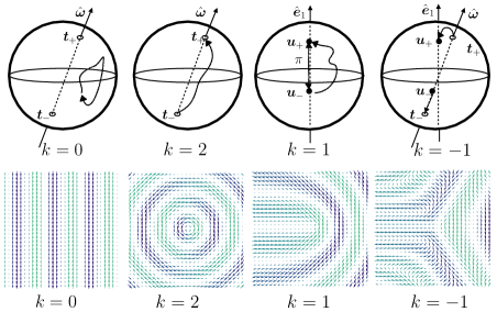
Figure 1: Topological defects (disclinations) with topological number $k$ in helical magnets. In the upper half different contours are shown as discussed in the text. The lower half shows the corresponding magnetization pattern in the $xy$-plane, as follows from eq.(8)

(i) In the simplest case a closed curve ${\bm{\omega}}(s)$ does not contain points ${\mathbf{t}}_{\pm}$ and ${\mathbf{u}}_{\pm}$. The path can therefore be continuously deformed into a point. The $\bm{\omega}$ rotation angle is therefore zero (see Fig.1a). There is no defect in this case.
(ii) A path which connects the points ${\mathbf{t}}_{-}$ and $\mathbf{t}_{+}$. It corresponds to the rotation angle $2\pi$ (see Fig.1b). In contrast to the case (i) this contour cannot be deformed into a point. The corresponding defect is called $2\pi$-disclination
(iii) Analogously a path which connects points $\mathbf{u}_{-}$ and $\mathbf{u}_{+}$ corresponds to the rotation angle $\pi$ (see Fig.1c) and corresponds to so-called $\pi$-disclination.
(iv) A closed curve that connects points ${\mathbf{u}}_{-},{\mathbf{u}}_{+}$ in a sequence $\bm{u}_{-}\to\bm{t}_{-}\sim\bm{t}_{+}\to\bm{u}_{+}$
(v) More complicated paths which touch equivalent points more than once can be continuously reduced to one of the cases (i)-(iv), as can be seen by explicit construction. A general linear defect in isotropic helical magnet corresponds to rotation to the angle $\pi[k]_{mod4}$ where $k$ is an integer.

As an example we consider contours $x(s),y(s)$ which include phase changes $k\pi$ about $\hat{\bm{\omega}}\equiv{\hat{\bm{e}}}_{1}$ by an angle

$$\theta[x(s),y(s)]=\frac{k}{2} \arctan\frac{y}{x} x>0$$ if

$$\theta[x(s),y(s)]=\frac{k}{2} \arctan\frac{y}{x}+\pi x<0$$ if . (7)

$\theta$ has a branch cut at $x=0,y\leq 0$. The rotated vectors are ${\hat{\bm{e}}}_{1}^{\prime}={\hat{\bm{e}}}_{1}\equiv\hat{\mathbf{z}}$, $\mathbf{q}^{\prime}=\mathbf{q}\cos\theta+{\hat{\bm{e}}}_{1}\times\mathbf{q}\sin\theta$ and hence

$$\mathbf{m}_{0}^{\prime}({\bm{r}}) = {\hat{\bm{e}}}\cos\mathbf{q}^{\prime}\cdot\mathbf{r}+\hat{\mathbf{q}}^{\prime}\times{\hat{\bm{e}}}_{1}\sin\mathbf{q}^{\prime}\cdot\mathbf{r}.$$ (8)

The function $\theta(x,y)$ has been used to create the magnetization profile in Fig. 1

III Domain walls in the bulk

Since the anisotropy allows several discrete orientations of the helix, wave vector domains with different helix orientation separated by domain walls (hDW) can appear. It was shown in Li 2012 that DWs in helical magnets are fundamentally different from common Bloch and Neel walls Bloch 1932 ; Neel 1948 . These DWs are one-dimensional textures in which magnetization rotates around a fixed axis. The hDWs are generically two-dimensional textures with rotating axis of rotation. For a range of orientations the hDWs contain a regular lattice of disclinations. The hDWs that are bisector planes between two helix wave vectors in different domains are free of disclinations and have minimal surface energy.

Let the helix wave vectors in two domains be $\mathbf{q}_{1}$ and $\mathbf{q}_{2}$. They are not collinear. In the bulk the angles between them is either $\pi/2$ if $v<0$ or $\arccos\frac{1}{3}$ if $v>0$. Since the asymptotic dependence of magnetization in two limiting cases cannot be described by one variable, the texture that connects the two asymptotical helixes must depend at least on two variables.

The second important fact is that the wave vector inside the domain wall necessarily changes its length. Indeed, any continuous distribution of magnetization can be described by function $\phi\left(\mathbf{r}\right)$ whose gradient is the local value of wave vector $\mathbf{q\left(r\right)=\nabla\phi\left(\mathbf{r}\right)}$. It is reasonable to assume that $\phi$ depends only on coordinates in the plane of the two wave vectors. In other words, the domain wall must be a plane perpendicular to the plane $\left(\mathbf{q}_{1},\mathbf{q}_{2}\right)$. Let us assume that the lines of wave vectors are continuous curves asymptotically approaching straight lines in direction $\mathbf{q}_{1}$ and $\mathbf{q}_{2}$ in different domains. Magnetization is described by eq. (2) in which the argument of sine and cosine is replaced by $\phi(\mathbf{r})$. It is possible to take unit vector $\hat{\mathbf{e}}_{1}$ perpendicular to the plane $\left(\mathbf{q}_{1},\mathbf{q}_{2}\right)$. The local vector $\hat{\mathbf{e}}_{2}\left(\mathbf{r}\right)$ is uniquely determined by the vectors $\mathbf{q}\left(\mathbf{r}\right)$ and $\hat{\mathbf{e}}_{1}$. The requirement of constant modulus for wave vector leads to equation $\left(\nabla\phi\right)^{2}=\mathrm{const}$. This equation coincides with the stationary Hamilton-Jacobi equation for free particle. The vector $\nabla\phi$ is the momentum of this particle. But free particle can not change its momentum. Therefore, there is no solution of such equation with asymptotics of $\nabla\phi$ equal to one constant vector in one domain and another constant vector in another domain.

Another consequence of this consideration is that the width of the hDW has the order of magnitude of the pitch of helix $\ell$. Indeed, the change of wave vector modulus violates the balance of exchange and DM forces. Namely they define the variation of magnetization inside the domain wall and restore theis balance outside. The contribution of anisotropy can be neglected. The only scale of the isotropic Hamiltonian is $\ell$. This peculiarity of the hDW is also unusual. Commonly the width of domain wall is determined by competition of exchange force and anisotropy. Such a domain wall would be much wider.

Consider the domain wall that is a bisector plane between vectors $\mathbf{q}_{1}$ and $\mathbf{q}_{2}$. Its normal is directed along the unit vector $\hat{\mathbf{q}}_{-}$ where

$$\mathbf{q}_{\pm}=\frac{1}{2}\left(\mathbf{q}_{1}\pm\mathbf{q}_{2}\right)$$ (9)

Both vectors $\mathbf{q}_{+}$ and $\mathbf{q}_{-}$ lay in the plane perpendicular to the domain wall. Let assume that vector field $\mathbf{q}\left(\mathbf{r}\right)$ asymptotically approaches $\mathbf{q}_{1}$ in the domain $\hat{\mathbf{q}}_{-}\cdot\bm{r}>0$ and $\mathbf{q}_{2}$ in the domain $\hat{\bm{q}}_{-}\cdot\bm{r}<0$.

A simple non-singular trial function for the phase $\phi\left(\mathbf{r}\right)$ in the presence of domain wall has a form:

$$\phi\left(\mathbf{r}\right)=\mathbf{q}_{+}\mathbf{r}+q_{-}w\ln\left[2\cosh\left(\frac{\mathbf{\hat{\mathbf{q}}_{-}\cdot r}}{w}\right)\right]$$ (10)

The vector field $\mathbf{q}\left(\mathbf{r}\right)$ for this trial function reads:

$$\mathbf{q\left(r\right)=}\mathbf{q}_{+}+\mathbf{q}_{-}\tanh\left(\frac{\mathbf{\hat{\mathbf{q}}_{-}\cdot{\bm{r}}}}{w}\right)$$ (11)

The magnetization in such texture can be represented as follows:

$$\mathbf{m\left(\mathit{x,y}\right)=}\hat{\mathbf{z}}\cos\phi\left(\mathbf{\mathit{x,y}}\right)+\hat{\mathbf{q}}\times\hat{\mathbf{z}}\sin\phi\left(\mathbf{\mathit{x,y}}\right)$$ (12)

Here $\hat{\mathbf{z}}$ is unit vector in the direction of vector $\mathbf{q}_{1}\times\mathbf{q}_{2}$, $\hat{\mathbf{q}}$ is unit vector in direction of $\mathbf{q\left(r\right)}$; $x-$axis is parallel to the vector $\mathbf{q}_{+}$. In Fig. 2 the regions of positive and negative projections of $\mathbf{m\left(r\right)}$ to the $z-$axis and local direction of $\mathbf{q\left(r\right)}$ are schematically shown for $w=0.3\ell$. Minimization of energy (see section 4) for mutually perpendicular $\mathbf{q}_{1}$ and $\mathbf{q}_{2}$ gives $w\approx 0.3\ell$. In order to make magnetic texture inside the hDW clearly visible we display in Fig. 2 a thicker domain wall.

Figure 2: Distribution of the magnetization projection $m_{z}$ in the bisector domain wall according to trial function (10) with $w=0.3\ell$. The value of $m_{z}$ is shown by color

Note that there are two bisectors for any pair of wave vectors in domains. Their trial functions differ by permutation of vectors $\mathbf{q}_{+}$ and $\mathbf{q}_{-}$. They both realize local angular minima of the surface energy, but their energies per unit area are different. Namely, the bisector of the angle $\alpha$ between wave vectors less than $\frac{\pi}{2}$ has smaller surface energy than bisector of complementary angle $\pi-\alpha$ (see Fig.3).

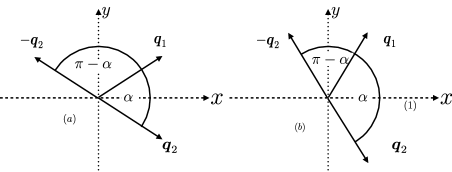
Figure 3: Wave vectors $\bm{q}_{1}$ and $\bm{q}_{2}$ and bisector domain walls (dashed or dotted).

Any attempt to extend such Ansatz to the case of domain wall of other orientation leads to divergent field $\mathbf{q\left(r\right)}$. The reason of that can be illustrated by example of mutually perpendicular $\mathbf{q}_{1}$ and $\mathbf{q}_{2}$ and the domain wall perpendicular to $\mathbf{q}_{1}$ and parallel to $\mathbf{q}_{2}$. Then in the plane of domain wall at approaching from the $\mathbf{q}_{1}$-domain, magnetization $\mathbf{m}$ is constant that means constant $\phi$, while at approaching from $\mathbf{q}_{2}$-domain, the phase is linear function of coordinates in plane and goes to infinity when coordinate $x$ goes to infinity. Since the transition from one asymptotic to another proceeds in the interval of finite width $\sim\ell$, $\left|\nabla\phi\right|$ also goes to infinity. This enormous mismatch can be avoided only by singularities that interrupt continuous counting of phase and allow to keep $\mathbf{q\left(r\right)}$ in finite limits. In our work Li 2012 we assumed that these compensating singularities are vortices or in terminology accepted for isotropic helical magnets (see section 2) $2\pi$-disclinations. However, as it was first understood by M. Garst Garst 2015 the $\pm\pi$-disclinations can do the same job with smaller energy price. Strictly speaking, disclinations are forbidden by discrete symmetry. However, they still can exist on a small length scale if their fields are compensated on distances much less than characteristic length at which the anisotropy becomes essential $\ell_{an}\sim\sqrt{J/v}a\sim\ell\frac{J}{g}$, i.e. in the range of 100 times larger than pitch.

Figure 4: Schematic plot of zig-zag domain wall formed by alternating $\pm\pi$-disclinations. The wave vectors near a separatrix are shown by arrows.

As it is clear from schematic picture Fig. 4 a periodic chain of $\pm\pi$-disclinations forms a zig-zag-shaped domain wall separating regions with mutually perpendicular wave vectors (one of them is parallel to the domain wall). In the work Li 2012 we predicted appearance of zig-zag domain walls. However, as the reason for zig-zag shape we indicated the instability of a domain wall whose orientation deviates from bisectors with respect to formation of a zig-zag whose sides are pieces of vortex-free domain walls, i.e. bisectors. Then two directions of zig-zag lines must be mutually perpendicular, whereas in the case of dominating disclination-anti-disclination structure the angle between them must be 120^∘. Zig-zag structure was first observed in experiments with alloy Fe_0.5Co_0.5Si.Uchida 2006 Fluctuations of the direction in these experiments were large and it is difficult to say what angle dominates. Topologically the vertex lines of zig-zag hDW are discilnations independently on what mechanism dominates. If the sides of zig-zag are large in comparison to pitch, both nechanisms can work at different scales. The most important new discovery made by the international team Schoenherr 2018 missed in our work Li 2012 is that the vertices of zig-zag are simultaneously centers of disclinations.

Let consider zig-zag structure in more details. It is possible to separate it in primitive cells each containing one $+\pi$ and one $-\pi$ disclinations. Each disclination has its own part of primitive cell either above upper vertex or below lower vertex of zig-zag. The parts belonging to different disclinations are separated by separatrices shown in Fig. 4 by dashed straight lines. Let us consider now two neighboring lower disclinations. Note that the angle between the wave vector and domain wall median plane ($x-$axis) near lower separatrix far from domain wall is equal to 0 for disclination left and $\pi$ for disclination right of separatrix. This seeming discontinuity in reality does not exist since these directions of wave vector are equivalent and magnetization remains continuous at separatrix. At a separatrix the phase $\phi$ experiences jump by $2\pi n$ with some integer $n$ that reduces it to the basic interval $(-\pi n,\pi n)$, but magnetization remains continuous. This is just the mechanism of mismatch compensation. In the range between upper and lower zig-zag vertices, there is no clear separation between the lines related to upper and lower disclinations. If the sides of zig-zag are significantly longer than the pitch, then the zig-zag sides can be considered as pieces of domain walls.

Let us calculate roughly the energy of the disclination hDW. With this purpose we will derive exact general equation for the domain wall energy as functional of the wave vector field $\mathbf{q\left(r\right)}$ that will be useful for other problems. Exchange energy is proportional to the square of tensor $\nabla\mathbf{m}$. According to eq. (12) components of this tensor read:

$$\partial_{\alpha}\mathbf{m}=q_{\alpha}\hat{\mathbf{q}}\times\mathbf{m}+\left(\partial_{\alpha}\hat{\mathbf{q}}\right)\times\hat{\mathbf{z}}\sin\phi$$ (13)

Vector $\partial_{\alpha}\hat{\mathbf{q}}$ is orthogonal to $\hat{\mathbf{q}}$. Therefore it is a linear combination $\partial_{\alpha}\hat{\mathbf{q}}=a\hat{\mathbf{z}}+b\hat{\mathbf{q}}\times\hat{\mathbf{z}}$. Since vector $\hat{\mathbf{q}}$ at any $\mathbf{r}$ lies in the $x,y$-plane, coefficient $a$ is zero. Thus $\partial_{\alpha}\hat{\mathbf{q}}\times\mathbf{z}=-b\hat{\mathbf{q}}$. It means that the first and second terms in the right hand side of eq. (13) are mutually orthogonal. Thus we find:

$$\left(\nabla\mathbf{m}\right)^{2}=\mathbf{q}^{2}+\sin^{2}\phi\left[\left(\partial_{\alpha}\hat{\mathbf{q}}\right)\times\hat{\mathbf{z}}\right]^{2}$$ (14)

Since $\partial_{\alpha}\hat{\mathbf{q}}$ is a vector perpendicular to $\hat{z}$, the expression $[\partial_{\alpha}\mathbf{q}\times z]^{2}$ can be replaced by $(\partial_{\alpha}\hat{\mathbf{q}})^{2}$. To calculate the DM energy we need to find curl of magnetization:

$$\nabla\times\mathbf{m}=-q\left(\mathbf{r}\right)\mathbf{m}+\hat{\mathbf{z}}\left(\nabla\hat{\mathbf{q}}\right)\sin\phi$$ (15)

and

$$\mathbf{m\cdot\nabla\times\mathbf{m}}=-q\left(\mathbf{r}\right)+\left(\nabla\hat{\mathbf{q}}\right)\sin\phi\cos\phi$$ (16)

Finally the total domain wall energy per unit area reads:

$$E_{dw}=\frac{J}{2L}\int_{0}^{L}dx\int_{-\infty}^{\infty}dy\left\{\left[q\left(\mathbf{r}\right)-q_{0}\right]^{2}+\frac{1}{2}\left(\partial_{\alpha}\hat{\mathbf{q}}\right)^{2}\right\},$$ (17)

where $L$ is period of zig-zag structure. The energy does not change if the phase 𝜙 in eq. (12) for magnetization changes by any constant. Therefore, in expression for energy the factor sin¿ 𝜙 of eq. (14) can be replaced by ½ and the second term of eq. (16) vanishes. Eq. (17) clearly demonstrates that domain wall energy consists of two independent parts. One of them is due to deviation of modulus of wave vector from its most energy favorable value $q_{0}$, whereas the second is due to change of its direction.

Applying this general equation to disclination domain wall, we conclude that square of deviation $\left[q\left(\mathbf{r}\right)-q_{0}\right]^{2}$ has order of magnitude $q_{0}^{2}$ inside domain wall and quickly decreases outside. Therefore integral from this term by order of magnitude is equal to $L^{2}q_{0}^{2}$. The second term in curl brackets due to rotation of wave vector is proportional to $1/r^{2}$ near each center of disclination, where $r$ is the distance to the center. After integration it gives $\ln\frac{L}{\ell}$ by order of magnitude. Thus, the total energy of disclination hDW per unit area is roughly equal to

$$E_{dw}\sim Jq_{0}^{2}L+J\frac{\ln\frac{L}{\ell}}{L}$$ (18)

Its minimization gives $L\sim q_{0}^{-1}\sim\ell$. More accurate coefficients in this relation can be found numerically. It requires sufficiently accurate solution of static Landau-Lifshitz equation with singularities or a proper trial function for $\phi(x,y)$ that we did not find so far.

IV Domain walls at crystal faces

In the cited work Schoenherr 2018 the authors studied about 90 samples of FeGe single crystals with typical sizes 0.5$\times$1$\times$1 mm. They were prepared by K. Nakamura under supervison of Y. Tokura by very slow (1 month) growth from vapors in vacuum quartz tube at temperature bias between 500 and 560^∘ C. The crystal structure was checked by Laue diffraction. The samples then were cut and polished to yield faces (100) and (110) with roughness 1 nm. MFM pictures and measurements were performed in Trondheim by P. Schoenherr under supervision of D. Meier. The magnetic tip in the MFM had radius about 50 nm. It was scanned with the distance of the tip to face 30 nm. Standard dual-pass MFM measurements allowed the resolution 10-15 nm. Measurements were performed at temperature 260-273K maintained by permanent water flux. M. Garst and A. Rosch supervised theoretical part of work.

The first experimental fact discovered in the MFM studies of helical magnet Schoenherr 2018 is that on the crystal face, the wave vectors of helix lay in the plane of face. That was checked for the faces (1,0,0) and (1,1,0). The second surprising fact is that unlike in the bulk, the orientation of the surface helix wave vector is not confined to a definite crystallographic directions within the face plane. These two facts can be explained if spin-orbit interaction near the face creates uniaxial easy-axis anisotropy. Let us denote $\mathbf{n}$ the normal vector to the face. Then surface anisotropy energy is

$$H_{sa}=-\lambda\int\mathbf{\left[n\cdot m\left(r\right)\right]}^{2}\frac{d^{2}x}{a^{2}}$$ (19)

The unit magnetization vector field is given by eq. (12). Let choose $\mathbf{e}_{1}=\frac{\mathbf{n\times}\mathbf{\hat{\mathbf{q}}}}{\left|\mathbf{n\times}\mathbf{\hat{\mathbf{q}}}\right|}$ and $\mathbf{e}_{2}=\mathbf{\hat{\mathbf{q}}\mathbf{\times e}_{1}}=\frac{\mathbf{n}-\hat{\mathbf{q}}\left(\mathbf{n\hat{\mathbf{q}}}\right)}{\left|\mathbf{n\times}\mathbf{\hat{\mathbf{q}}}\right|}$. Then $\mathbf{nm\left(r\right)}=\mathbf{ne_{2}\sin\phi\left(\mathbf{r}\right)}=\left|\mathbf{n\times}\mathbf{\hat{\mathbf{q}}}\right|\sin\phi\left(\mathbf{r}\right)$. Average $\left\langle\mathbf{\left[n\cdot m\left(r\right)\right]}^{2}\right\rangle$ over phase $\phi$ is equal to $\frac{1}{2}\left(\mathbf{n\times}\mathbf{\hat{\mathbf{q}}}\right)^{2}=\sin^{2}\theta$ where $\theta$ is the angle between helix wave vector $\mathbf{q}$ and the normal to the face $\mathbf{n}$. Thus, the surface anisotropy energy per unit area is $\sigma=-\frac{\lambda}{2}\sin^{2}\theta$. It has minimum at $\theta=\frac{\pi}{2}$, i.e. for the helix wave vector in the plane of face. The value of surface anisotropy $\lambda$ appears as relativistic correction of the second order, whereas the constant of cubic anisotropy $v$ appears only in the fourth order relativistic correction. Therefore it is reasonable to assume that $\lambda\gg v$. This fact explains why the helix wave vector tends to turn parallel to the face plane. The in-face anisotropy is too weak to confine these vectors to crystal directions with small indices in the face. In infinite perfect samples the helix vector on surface is determined by its bulk value and the normal to the face with some exceptions. For the face (001) and the same helix wave vector in the bulk, any direction of surface helix wave vector has the same energy. The authors of article Schoenherr 2018 concluded that there is no dependence between bulk and surface wave vectors. When the bulk vector is not perpendicular to the crystal face as happens for the face (110), this result looks surprising. It may happen if the parameters $J$ and $g$ rapidly change in close vicinity of the boundary. Then surface layer becomes to some extent magnetically independent of the bulk. An alternative explanation proposed in Schoenherr 2018 is the closeness of temperature 260-273 K at which measurements were performed to the Neel point $T_{N}=278K$. In this range of temperature the magnetization is still small and energy of bulk anisotropy proportional to the fourth power of magnetization becomes negligible in comparison to other contribution to energy quadratic in $\mathbf{m}$.

Due to insensitivity of energy to the direction of surface helix wave vectors, the angle $\alpha$ between wave vectors $\mathbf{q}_{1}$ and $\mathbf{q}_{2}$ in different domains changes from sample to sample. Symmetry of wave vectors with respect to change of sign implies that $\alpha$ varies in the limits between 0 and $\pi$. Let us denote $\beta$ the angle formed by one of the helix wave vectors and domain wall. Experimental graph of dependence of $\beta$ on $\alpha$ is shown in Fig. 5d.

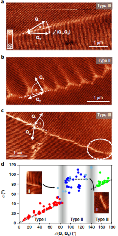
Figure 5: MFM pictures of Helimagnetic domain walls in FeGe. Reproduced from article Schoenherr 2018 by courtesy of Profs. D. Meier and Y. Tokura. a. Bisector domain wall at $\alpha<80^{\circ}$ (type I); b. Zig-zag disclination wall (type III);c. Bisector domain wall at $\alpha>140^{\circ}$ (dislocation wall, type II); d. Graph of the angle $\beta$ between domain wall and one of the helix wave vectors (our notations differ from those accepted in Schoenherr 2018 ). See comments in the text.

It shows that at $0<\alpha<80$^∘ (DW of the type I in terminology accepted in Schoenherr 2018 ) and at 140^∘$<\alpha<180$^∘ (DW of type III), $\beta$ follows well defined dependence $\beta=\alpha/2.$ These are domain walls whose plane are bisectors between vectors $\mathbf{q}_{1}$ and $\mathbf{q}_{2}$ that are well described by variational eqs. (10,11). Experimental data imply that domain walls in this ranges of $\alpha$ relax to the closest bisector direction. Note that the angle between any possible initial direction of the hDW and bisector in this range of angles is less than 40^∘. In the interval 140^∘$<\alpha<180$^∘ (DW of the type II), $\beta$ is not a function of $\alpha.$ Experimental values of $\beta$ at fixed $\alpha$ are scattered in this range of $\alpha$ more or less uniformly between $\alpha/2$ and $\alpha$. Such domain walls must be supplied with zig-zag chain of disclinations-antidisclinations as discussed in Section 3. However, at $\alpha=90$^∘ and a fixed value $\beta\neq 0,\frac{\pi}{2}$, the two lines within a primitive period have different lengths. It follows from geometrical constraints, i.e. fixed values $\alpha$ and $\beta$ and angles (120^∘ or 90^∘) at vertices of zig-zag line. MFM pictures of the domain walls in this range of $\alpha$ confirm the existence of disclination-antidisclination zig-zag structure, though in real crystals it is not so ideally periodic and domain wall median is not ideal straight line

In theoretical part of the article Schoenherr 2018 , the authors performed micromagnetic calculations of domain wall configuration in two dimensions. They demonstrated that at small and large angles $\alpha$, minimum energy is realized by smooth non-singular bisector domain walls. At angles $\alpha$ in the range near 90^∘, the domain walls has zig-zag shape with regularly intermitting disclinations and anti-disclinations. Theory even describes the irregularity of this chain considering them as random fluctuations. This is without doubt a success. However some principal questions remain unanswered.

The main such question is what keeps orientation of the helix wave vectors? We understand that in the bulk it is anisotropy that reduces initial SO(3) symmetry of the exchange and DM interactions to discrete group of cube without inversion. But experimenters tell us that anisotropy plays no role at the crystal faces. Then there is no topological reason for appearance of domain walls. Another idea is that the helix on the surface is fixed by its coupling with the helix in the bulk. In this case orientation of the wave vector at the surface could be arbitrary in plane of the face (001), but not in the face (110). It also may be the edge or random pinning that fixes the orientation of wave vector near the boundaries or defects and then these fixed pieces serve as nuclei for domain growth.

But if the direction of helix vector can vary continuously another principal question appears. If symmetry of a system does not require domain walls as topological defects, can they nevertheless appear if different possible values of order parameter are fixed ’by hands” near boundaries of the sample? For simple systems such as Heisenberg or XY (planar) magnets the answer to this question is no. In both cases, if spins on two sides of a big stripe or slab are fixed artificially, the transition from one to another orientation in the sample proceeds smoothly. Instead of domain wall we see spins slowly rotating in space. The principal question is whether the same is correct for an isotropic helical magnets. The difference with simpler systems is that there is no smooth texture that changes its direction conserving the modulus of wave vector (see Section 3). In this article we issue a proof of the statement that in isotropic helical magnet, the transition between two different helix wave vectors fixed near boundaries proceeds by formation of the hDW whose width depends on the angle $\alpha$ between fixed wave vectors. We calculate explicitly the angular dependence of the width for bisector domain walls given by variational ansatz (10).

The derivation of this result employs general equation (17) with $\mathbf{q}(\mathbf{r})$ given by Ansatz (11). It represents the domain wall energy as a sum of two positive contributions $E_{dw}^{(1)}$ and $E_{dw}^{(2)}$ originating from deviation of $q(\mathbf{r})$ from its energy preferable value $q_{0}$ and from rotation of the wave vector $\hat{\mathbf{q}}(\mathbf{r})$, respectively. The integrals involved in these expressions can be calculated explicitly. The result is as follows:

$$E_{dw}^{(1)}=\frac{1}{2}Jq_{0}^{2}wI_{1},$$ (20)

where

$$I_{1}(\alpha) = \frac{\sin\alpha}{2}\left(-\frac{a^{2}-1}{a}+A\ln a+B\ln\frac{2a}{a^{2}+1}\right)$$ (21)

and

$$a = \cot\frac{\pi-\alpha}{4},\,\,A=\frac{2\left(a^{2}+1\right)}{a},\,\,B=\frac{2\left(a^{2}+1\right)^{2}}{a\left(a^{2}-1\right)}.$$ (22)

The rotational part of energy reads $E_{dw}^{(2)}=\frac{J}{w}I_{2}$ where

$$I_{2}(\alpha)=\frac{1}{2}\left(\alpha-\cot\alpha\right)$$ (23)

Minimization of the total DW energy $E_{dw}=E_{dw}^{(1)}+E_{dw}^{(2)}$ over $w$ leads to the result:

$$w(\alpha)=q_{0}^{-1}\sqrt{\frac{I_{2}}{I_{1}}}$$ (24)

This equation shows that the width of bisector domain wall becomes infinite at $\alpha=0$, has a minimum and again goes to infinity at $\alpha=\pi$. The curve $w(\alpha)$ (see Fig. 5) is not symmetric with respect to the point $\alpha=\pi/2$, i.e. $w(\alpha)\neq w(\pi-\alpha)$. This asymmetry seemingly contradicts to the established invariance of the helix to the flip of one of wave vectors. The reason of this asymmetry is the accepted assumption that domain wall is the bisector of a smaller angle between wave vectors entire interval $0<\alpha<\pi$. Certainly, the second half of this interval can be reduced to the first by the flip, for definiteness, of $\mathbf{q}_{2}$, i.e. by transformation $\alpha\leftrightarrow\pi-\alpha$. However, at this flip the domain wall that forms an angle $\pm(\pi-\alpha)/2$ with wave vectors is bisector of not the smaller, but larger angle between two axis of rotations (see Fig. 3).

More formally this fact can be formulated as follows: at accepted assumption, the symmetry transformation is $\alpha\leftrightarrow\pi-\alpha$ and simultaneously $\mathbf{q}_{+}\leftrightarrow\mathbf{q}_{-}$. As we stated earlier, the surface energy of the bisector of larger angle hDW is larger than the analogous energy for smaller angle. Note that both are local minima of the surface energy $\sigma$ as function of the angle $\beta$ between plane of domain wall and one of the wave vectors at fixed value of $\alpha$. In the bulk the angle between different wave vectors is $\alpha=\frac{\pi}{2}$. Then $a=\sqrt{2}+1\approx 2.414$ and the domain wall width of bisector domain wall is $w\left(\pi/2\right)\approx 0.038\ell$.

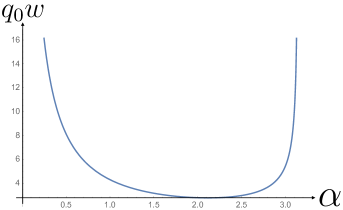
Figure 6: Graph of function $\sqrt{2}q_{0}w(\alpha)$ for the width of bisector hDW.

Though our calculation relates to a specific choice of trial function, the main features of the function $w(\alpha)$ minimizing the surface energy remains the same for exact solution of this problem. Namely, $w(\alpha)\rightarrow\infty$ at $\alpha\rightarrow 0$ and $\alpha\rightarrow\pi$; it has minimum and it goes to infinity at $\alpha=\pi/2$. It is asymmetric with respect to reflection in the point $\alpha=\pi/2$. At this value of $\alpha$, both angles between axis of rotations are equal. Therefore, in this case the width and the energy of two branches of the curves $w(a)$ and $E(\alpha)$ arrive at the common limit.

We start the proof of these statements with the case of small $\alpha$. In general case the wave vector $\mathbf{q}(x,y)$ must go to the limit $\hat{x}q_{0}$ at $\alpha\rightarrow 0$. Corrections to this limit at small $\alpha$ must start at least with $\alpha^{2}$ since at permutation of two wave vectors the distribution of magnetization does not change. It means that modulus of wave vector $q(x,y)$ differs from $q_{0}$ by a small value of the relative order $\alpha^{2}$. As a consequence $|q(x,y)-q_{0}|^{2}$ has order of magnitude $\alpha^{4}q_{0}^{2}$ and $I_{1}\sim\alpha^{4}$. The unit vector $\hat{\mathbf{q}}(x,y)$ rotates in the domain wall to the angle $\alpha$. Therefore, $\nabla\hat{\mathbf{q}}$ is $\sim\alpha/w$ by the order of magnitude. Thus, $I_{2}\sim\alpha^{2}$. We conclude that $w(\alpha)\propto 1/\alpha$ at $\alpha\rightarrow 0$.

At $\alpha$ approaching $\pi$, the $x-$component of wave vector tends to zero. Neglecting it, we arrive at wave vector that has only $y-$ component. Due to symmetry, it changes sign at crossing the median of hDW $y=0$. Therefore, the unit vector of its direction is equall to sign of $y$ and its derivative $\nabla\hat{\mathbf{q}}=2\delta(y)$. Thus, $I_{2}=w\int_{0}^{\infty}(\nabla\hat{\mathbf{q}})^{2}d\eta$ diverges at $\alpha$ approaching $\pi$. On the other hand, integral $I_{1}$ remains finite in this limit since $q$ is even function of $y$ that becomes zero at $y=0$ and tends to the value $q_{0}$ at $y\rightarrow\pm\infty$. Thus $|q-q_{0}|$ has maximum equal to $q_{0}$ at $y=0$ and rapidly decreases outside domain wall.

Let consider briefly the energetics of domain walls. It follows from exact equation valid for bisector hDW’s and is not associated with any variational ansatz:

$$E_{dw}=Jq_{0}\sqrt{I_{1}I_{2}}.$$ (25)

From previous analysis we find that at $\alpha\rightarrow 0$, the surface energy of the bisector hDW goes to zero as $|\alpha|^{3}$. At $\alpha=\rightarrow\pi$ this energy becomes infinite. This result seems to be inconsistent with equivalence of $\alpha=\pi$ and $\alpha=0$. However, as we have shown earlier , just at the value of $\alpha=\pi$, $x-$component of wave vector is equal to zero at any $x$ and $y$, whereas its $y$-component turns into zero at the median of the hDW. Thus, the limit of the bisector hDW at $\alpha\rightarrow\pi$ leads to the specific minimization problem for a helical configuration with wave vector directed everywhere along $y-$axis, changing from $-q_{0}$ to $q_{0}$ and taking value 0 at $y=0$. Energy of such configuration is infinite as we have shown earlier.

The micromagnetic calculations in Schoenherr 2018 qualitatively agree with our consideration in the range $0<\alpha<80$^∘, though quantitatively this dependence is closer to $\alpha^{2}$ instead of our result $\alpha^{3}$. But in the second range of bisector hDW $140$^∘$<\alpha<180$^∘ it results in monotonic decrease of surface energy to zero value at $\alpha=\pi$ in contrast to infinite surface energy predicted by our theory. The reason of these discrepancies presumably is the finite size of a ”sample” used in micromagnetic calculations. It does not exceed $20\ell$. It becomes smaller than the width of the domain wall at $\alpha$ sufficiently close to 0 or $\pi$ invalidating the calculation of surface energy.

As for zig-zag domain walls we have seen already that at $\alpha=90$^∘ and $\beta=0$, zig-zag line is symmetric, its sides have equal length. Therefore it could be expected that it realizes minimum of energy in comparison with either $\beta\neq 0$ or $\alpha\neq 90$^∘. Indeed such a minimum was found in the same micromagnetic calculations. However, energetically unfavorable configuration do not relax to this energy minimum. The metastability of these configurations may be associated with their complicated topological structure and small distances between disclinations and antidisclinations that increase their rigidity.

In conclusion of this section we propose an approach to the problem of zig-zag domain walls at arbitrary angle $\alpha$ between the wave vectors in the two domains based on its similarity with the devils staircase in the commenurate-incommensurate transition Pokrovsky 1983 . Let consider a domain wall tilted with the angle $\gamma=\beta-\alpha/2$ to the direction of bisector. As we have seen already, such a tilt leads to a mismatch between periods of upper and lower helixes at their crossing with domain wall. These periods are $l_{i}=\ell/\cos(\alpha/2\mp\gamma);\,i=1,2$. The mismatch sums up to a full period if $(n+1)l_{1}=nl_{2}$ (we considered the simplest commensurate situation). This condition is satisfied if $\gamma=\gamma_{n}=\arctan[\cot(\frac{\alpha}{2n+1})]$. The mismatch can be avoided by introduction of a pair $\pm\pi$-disclinations. The distance between two such dipoles must be $L=n\ell$. Let the distance between two disclination in the dipole is $d$. The mismatch though small ($q-q_{0}\propto\alpha\gamma q_{0}$ at small $\alpha$ and $\gamma$) persists at least at the distance $L$ generating the deviation energy of the order $J(\gamma q_{0}\alpha d)^{2}/L$ per unit area. The rotation energy per unit area is $\sim J\alpha^{2}[\ln(L/d)]/L$. Minimization over $d$ gives $d\sim\ell/\gamma^{2}$, but the energy decreases with $L$. We conclude that in the infinite system $L$ must be infinite at small angles $\alpha$ and $\beta$. Thus, we have proved that the domain wall tilted to bisector at small angle $\gamma$ are unstable. This stament agrees with experiment Schoenherr 2018 that did not observe such domain walls at small $\alpha$. The situation is different at large angles $\alpha$ and $\gamma$ since in this case the only scale of length for the hDW is $L$.

Schönherr et al. Schoenherr 2018 argued theoretically and have shown numerically that surface energy of the disclination hDW has minimum at angle between wave vectors $\alpha=\pi/2$ and $\beta=\gamma=0$. Our consideration shows that it should have more shallow minima at the same $\alpha$ and an infinite discrete set of $\gamma=\gamma_{n}$ corresponding to simple rational mismatch. Another rational mismatches of two steps of zig-zag and also zig-zags consisting of more than two steps would give a Devil’s staircase of local minima, but only few of them with minimal denominators will be seen at finite temperature.

V Conclusions

Here we discuss open questions. Some of them are related to experiment. It would be very instructive to perform measurements on the same or other samples, but at temperature lower than 260K in FeGe to ensure that the volume anisotropy is more significant. Will arbitrary directions of wave vectors and angles between them persist? It would be also interesting to apply polarized electron or neutron scattering to get information on the same objects not only at the surface, but at least partly in the bulk. Though the samples used in experiment Schoenherr 2018 were sufficiently large, there were no long regular hDW on presented pictures. This fact interferes quantitative comparison of theory and experiment.

Among theoretical problems we would like to mention, first is the problem of the bulk-surface coupling or decoupling. So far there is no satisfactory theory of this phenomenon. It is very important to develop variational methods for structure and energy of the hDWs with the goal to get a desirable precision. So far we even could not compare our variational calculations of bisector domain walls made for infinite sample with micromagnetic calculations in Schoenherr 2018 since the latter were performed for finite and not too large samples. Their authors have found significant finite size effects. Thus, it would be useful to develop variational approach to finite samples. Variational approach to theory of disclination domain walls so far did not achieve quantiative level. We are looking now for a satisfactory trial function for magnetization.

Important statements that were proved in this article include stability of the smooth (bisector) domain walls at all angles between wave vectors and instability of zig-zag domain walls at small angles.

VI Acknowledgenents

This work was supported by the University of Cologne Center of Excellence QM2 and by William R. Thurman’58 Chair in Physics, Texas A&M University. We are thankful to Prof. D. Meier or very useful discussion of experimental procedure and sending us the original version of Fig. 5. Our thanks due to him and Prof. Y. Tokura for kind permission to use experimental figures from article Schoenherr 2018 and to Dr. Chen Sun for his courteous help in preparation of Fig. 2.

References

- (1) F. Li, T. Nattermann and V.L. Pokrovsky, Phys. Rev. Lett. 108, 107203 (2012).
- (2) P. Schönherr, J. Müller, L. Köhler, A. Rosch, N. Kanazawa, Y. Tokura, M. Garst, D. Meier, Nature Physics Letters, online, March 5, 2018.
- (3) G. Toulouse, G. and M. Kleman, J. de Phys.-Lettres 37, L-149 (1976).
- (4) G.E. Volovik and V.P. Mineev, Sov. Phys. JETP 45, 1186 (1977).
- (5) P.M. Chaikin and T.C. Lubensky, Principles of Condensed Matter Physics, Cambridge Univ. Press, 1995.
- (6) G.E. Volovik, The Universe in a helium droplet, Oxford Univ. Press, 2003
- (7) A.M. Polyakov, Gauge fields and strings, Harwood Academic Publishers, Chur, 1987.
- (8) A.A. Abrikosov, Sov. Phys. JETP 5, 1174 (1957).
- (9) L. Onsager, Nuovo Cimento 6, suppl. 2, 249 (1949).
- (10) Feynman, R. P. , Application of quantum mechanics to liquid helium. Progress in Low Temperature Physics, 1: 17–53, (1955).
- (11) H.P. Haasen, Berichte, Gött. Akad. Wiss. 1210, 107 (1971).
- (12) P.W. Anderson, Basic notions in condensed matter physics, Benjamin Cummings, 1984.
- (13) T. H.R. Skyrme, Nuclear Physics. 31, 556–569 (1962).
- (14) A.A. Belavin and A.M. Polyakov, JETP Lett. 22, 245–248 (1975).
- (15) A. Abanov, V.L. Pokrovsky, Skyrmion in a real magnetic film, Phys. Rev. B, 58 (1998) R8889-R8892.
- (16) A. Bogdanov and A. Hubert, J. Magn. Magn. Mater. 138, 255 (1994).
- (17) N.S. Kiselev, A.N. Bogdanov, R. Schäfer, U.K. Rößler, Journal of Physics D: Applied Physics, 44 (39) 392001(2011).
- (18) S. Mühlbauer, B. Binz, F. Jonietz, C. Peiderer, A. Rosch, A. Neubauer, R. Georgii, and P. Böni, Science 323, 915 (2009)
- (19) X. Z. Yu, Y. Onose, N. Kanazawa, J. H. Park, J. H. Han, Y. Matsui, N. Nagaosa, and Y. Tokura, Nature 465, 901 (2010)
- (20) Albert Fert, Nicolas Reyren, V. Cros, Nat. Rev. Mater., 2, 17031 (2017).
- (21) G.E. Volovik, Exotic Properties of Superfluid 3He, World Scientific, 1992.
- (22) S. M. Mühlbauer et al., Nature (London) 427, 227 (2004).
- (23) M. Uchida et al., Phys. Rev. B 77, 184402 (2008).
- (24) M. Uchida, Y. Onose, Y. Matsui, and Y. Tokura, Science 311, 359 (2006).
- (25) B.Lebech, J. Bernhard and T. Freltoft, J. Phys. Condens. Matter 1, 6105 (1989).
- (26) F. Bloch, Z. Phys. 74, 295 (1932).
- (27) L. Neel, Annales de Physique 3, 137(1948).
- (28) M. Garst, private communication (2015).
- (29) V.L. Pokrovsky and A.L. Talapov, Theorie of Incommensurate crystals, Harwood Academic Publishers, Chur, 1983; I. Lyksyutov, A.G. Naumovets and V. Pokrovsky, Two-Dimensional Crystals, Academic Press, Boston, 1983.