Taming VAEs
Abstract
In spite of remarkable progress in deep latent variable generative modeling, training still remains a challenge due to a combination of optimization and generalization issues. In practice, a combination of heuristic algorithms (such as hand-crafted annealing of KL-terms) is often used in order to achieve the desired results, but such solutions are not robust to changes in model architecture or dataset. The best settings can often vary dramatically from one problem to another, which requires doing expensive parameter sweeps for each new case. Here we develop on the idea of training VAEs with additional constraints as a way to control their behaviour. We first present a detailed theoretical analysis of constrained VAEs, expanding our understanding of how these models work. We then introduce and analyze a practical algorithm termed Generalized ELBO with Constrained Optimization, GECO. The main advantage of GECO for the machine learning practitioner is a more intuitive, yet principled, process of tuning the loss. This involves defining of a set of constraints, which typically have an explicit relation to the desired model performance, in contrast to tweaking abstract hyper-parameters which implicitly affect the model behavior. Encouraging experimental results in several standard datasets indicate that GECO is a very robust and effective tool to balance reconstruction and compression constraints.
1 Introduction
Deep variational auto-encoders (VAEs) have made substantial progress in the last few years on modelling complex data such as images Kingma2013AutoEncodingVB ; Rezende2014StochasticBA ; Kingma2016ImprovedVI ; Snderby2016LadderVA ; Gregor2016TowardsCC ; Gulrajani2016PixelVAEAL ; Bachman2016AnAF , speech synthesis akuzawa2018expressive ; hsu2017learning , molecular discovery gomez2016automatic ; sultan2018transferable ; hernandez2017variational , robotics inoue2017transfer ; park2018multimodal ; van2016stable and 3d-scene understanding GQN ; rezende2016unsupervised ; eslami2016attend .
VAEs are latent-variable generative models that define a joint density between some observed data and unobserved or latent variables . The most popular method for training these models is through stochastic amortized variational approximations Rezende2014StochasticBA ; Kingma2013AutoEncodingVB , which use a variational posterior (also referred to as encoder), , to construct the evidence lower-bound (ELBO) objective function.
One prominent limitation of vanilla VAEs is the use of simple diagonal Gaussian posterior approximations. It has been observed empirically that VAEs with simple posterior models have a tendency to ignore some of the latent-variables (latent-collapse) Tomczak2018VAEWA ; Burda2015ImportanceWA and produce blurred reconstructions Burda2015ImportanceWA ; Snderby2016LadderVA . As a result, several mechanisms have been proposed to increase the expressiveness of the variational posterior density Nalisnick2016ApproximateIF ; Rezende2015VariationalIW ; Salimans2015MarkovCM ; Tomczak2016ImprovingVA ; Tran2015TheVG ; Kingma2016ImprovedVI ; Berg2018SylvesterNF ; Gregor2016TowardsCC but it still remains a challenge to train complex encoders due to a combination of optimization and generalization issues Cremer2018InferenceSI ; Rosca2018DistributionMI . Some of these issues have been partially addressed in the literature through heuristics, such as hand-crafted annealing of the KL-term GQN ; Snderby2016LadderVA ; Gregor2016TowardsCC , injection of uniform noise to the pixels theis2015note and reduction of the bit-depth of the data. A case of interest are VAEs with information bottleneck constraints such as -VAEs Higgins2016vaeLB . While a body of work on information bottleneck has primarily focused on tools to analyze models Alemi2017FixingAB ; tishby2000information ; tishby2015deep , it has also been shown that VAEs with various information bottleneck constraints can trade off reconstruction accuracy for better-factorized latent representations Higgins2016vaeLB ; Burgess2018UnderstandingDI ; Alemi2016DeepVI , a highly desired property in many real-world applications as well as model analysis. Other types of constraints have also been used to improve sample quality and reduce latent-collapse zhao2017towards , but while using supplementary constraints in VAEs has produced encouraging empirical results, we find that there have been fewer efforts towards general tools and theoretical analysis for constrained VAEs at scale.
Here, we introduce a practical mechanism for controlling the balance between compression (KL minimization) and other constraints we wish to enforce in our model (not limited to, but including reconstruction error) termed Generalized ELBO with Constrained Optimization, GECO. GECO enables an intuitive, yet principled, work-flow for tuning loss functions. This involves the definition of a set of constraints, which typically have an explicit relation to the desired model performance, in constrast to tweaking abstract information-theoretic hyper-parameters which implicitly affect the model behavior. In spite of its simplicity, our experiments support the view that GECO is an empowering tool and we argue that it has enabled us to have an unprecedented level of control over the properties and robustness of complex models such as ConvDraw Gregor2016TowardsCC ; GQN and VAEs with NVP posteriors Rosca2018DistributionMI .
The key contributions of this paper are: (a) With a focus on ELBOs with supplementary constraints, we present a detailed theoretical analysis of the behaviour of high-capacity VAEs with and without KL and Lipschitz constraints, advancing our understanding of VAEs on multiple fronts: (i) We demonstrate that the posterior density of unconstrained VAEs will converge to an equiprobable partition of the latent-space; (ii) We provide a connection between -VAEs and spectral clustering; (iii) Drawing from statistical mechanics we study phase-transitions in the reconstruction fixed-points of -VAEs; (b) Equipped with a better understanding of the impact of constraints in VAEs, we design the GECO algorithm.
The remainder of the paper is structured as follows: in Section 3.1 we study the behavior of unconstrained VAEs at convergence; in Section 3.2 we draw links between -VAEs and spectral clustering, and we study phase-transitions in -VAEs; in Section 3.4 we present the GECO algorithm; finally, in Section 4 we illustrate our theoretical analysis on mixture data and we assess the behavior of GECO on several larger datasets and for different types of constraints.
2 Related work
,Similarly to zhao2017towards we study VAEs with supplementary constraints in addition to the ELBO objective function and we study its behaviour in the information plane as in Alemi2017FixingAB . Our theoretical analysis extends the analysis performed in zhao2017towards ; Alemi2017FixingAB with an emphasis on the properties of the learned posterior densities in high-capacity VAEs. Our analysis also extends the idea of information bottleneck and geometrical clustering from strouse2017information to the case where latent variables are continuous instead of discrete. A further extension of the analysis including the incorporation of Lipschitz constraints is also available in Appendix B. Complementary to the analysis from Dai2017HiddenTO with (semi-)affine assumptions on the VAE’s decoder, we focus on non-linear aspects of high-capacity constrained VAEs.
GECO is a simple mechanism for approximately optimizing VAEs under different types of constraint. It is inspired by the empirical observation that some high-capacity VAEs such as ConvDRAWGregor2016TowardsCC ; GQN may reach much lower reconstruction errors compared to a level that is perceptually distinguishable, at the expense of a weak compression rate (large KL). GECO is designed to be an easy-to-implement and tune approximation of more complex stochastic constrained optimization techniques wang2003stochastic ; rocha2010stochastic and to take advantage of the reparametrization trick in VAEs Kingma2013AutoEncodingVB ; Rezende2014StochasticBA . At a high-level, GECO is similar to information constraints studied in Alemi2017FixingAB ; phuong2018the ; Zhang2017InformationPA ; Kolchinsky2017NonlinearIB . However, we argue that in many practical cases it is much easier to decide on useful constraints in the data-domain, such as a desired reconstruction accuracy, rather than information constraints. Additionally, the types of information constraints we can impose on VAEs are restricted to a few combinations of KL-divergences (e.g. mutual information between latents and data), whereas there are many easily available ways of meaningfully constraining reconstructions (e.g. bounding reconstruction errors, bounding the ability of a classifier to correctly classify reconstructions or bounding reconstruction errors in some feature space).
Some widespread practices for modelling images such as injecting uniform noise to the pixels and reducing the bit-depth of the color channels (e.g. theis2015note ; kingma2018glow ; Gregor2016TowardsCC ; Rosca2018DistributionMI ) can also be mathematically interpreted as constraints which bound the values of the likelihood from above. For instance, training a model with density by injecting uniform noise to the samples is a way of maximizing the likelihood under the constraint . With GECO, there is no need to resort to these heuristics.
3 Methods
VAEs are smooth parametric latent variable models of the form and are trained typically by maximizing the ELBO variational objective, , using a parametric variational posterior .
| (1) |
where the prior is taken to be a unit Gaussian and the empirical data density is represented as , where are the training data-points.
We focus on VAEs with Gaussian decoder density of the form , where is a global parameter and is referred to as a decoder or generator. Restricting to decoder densities where the components of are conditionally independent given a latent vector eliminates a family of solutions in the infinite-capacity limit where the decoder density ignores the latent variables, i.e. , as observed in Alemi2017FixingAB . This restriction is important because we are interested in the behaviour of the latent variables in this paper.
In contrast to ELBO maximization, we consider a constrained optimization problem for variational auto-encoders where we seek to minimize the KL-divergence, , under a set of expectation inequality constraints of the form where . We refer to this type of constraint as reconstruction constraint since they are based on some comparison between a data-point and its reconstruction. We can solve this problem by using a standard method of Lagrange multipliers, where we introduce the Lagrange multipliers and optimize the Lagrangian via a min-max optimization scheme bertsekas1996 ,
| (2) |
A general algorithm for finding the extreme points of the ELBO and of the Lagrangian is provided in Proposition 1, where we extend the well-known derivations from rate-distortion theory blahut1972computation ; csisz1984information ; cover2012elements ; tishby2000information to the case with reconstructions constraints.
Proposition 1.
(Fixed-point equations) The extrema of the ELBO with respect to the decoder and encoder are solutions of the fixed-point Equations 3 and 4 and for the Lagrangian , Equations 5 and 6 respectively
| (3) | ||||
| (4) | ||||
| (5) | ||||
| (6) |
where , and . See proof in Section C.1.
In the following Sections 3.1 and 3.2 we analyze properties of Equations 3, 4, 5 and 6 constraints to gain a better understanding of the behaviour of VAEs. In Appendix B we also provide additional analysis of the effect of local and global Lipschitz constraints for the interested reader.
3.1 Unconstrained VAEs
In the unconstrained case, where we optimize the ELBO, we can derive a few interesting conclusions from Equations 3 and 4: (i) The global optimal decoder is a convex linear combination of the training data of the form ; (ii) If we optimize the standard-deviation jointly with the decoder and encoder, it will converge to zero; (iii) The posterior density will converge to a distribution with support corresponding to one element of a partition of the latent space. Moreover, the set of supports of the posterior density formed by each data-point constitutes a partition of the latent space that is equiprobable under the prior. These results are formalized in Proposition 2, where we demonstrate that a solution satisfying all these properties is a fixed point of Equations 3 and 4.
Proposition 2.
(High-capacity VAEs learn an equiprobable partition of the latent space): Let , where is a normalization constant, be the variational posterior density, evaluated at a training point . This density is equal to the restriction of the prior to a limited support in the latent space. is a fixed-point of equations (5) for any set of volumes that form a partition of the latent space. Furthermore, the highest ELBO is achieved when the partition is equiprobable under the prior. That is, , and if . See proof in Section C.2.
The fact that the standard deviation will converge to results in a numerically ill-posed problem as observed in Mattei2018LeveragingTE . Nevertheless, the fixed-point equations still admits a stationary solution where the VAE becomes a mixture of Dirac-delta densities centered at the training data-points.
It is known empirically that low-capacity VAEs tend to produce blurred reconstructions and samples zhao2017towards ; Higgins2016vaeLB . Contrary to a popularly held belief (e.g. nowozin2016f ), this phenomenon is not caused by using a Gaussian likelihood alone: as observed in zhao2017towards , this is primarily caused by a sub-optimal variational posterior. The fixed-point equation (4) provides a mathematical explanation for this phenomenon, generalizing the result from zhao2017towards : the optimal decoder for a given encoder is a convex linear combination of the training data. If the VAE’s encoder cannot accurately distinguish between multiple training data-points, the resulting weights in the VAE’s decoder will be spread across the same data-points, resulting in a blurred reconstruction. This is formalized in Proposition 3.
Proposition 3.
(Blurred reconstructions) If the supports from Proposition 2 are overlapping (i.e. for ), then the optimal reconstruction at a latent point for a fixed encoder will be the average of all data-points mapping to any of the overlapping basis weighted by the inverse prior probability of the respective basis. See proof in Section C.3.
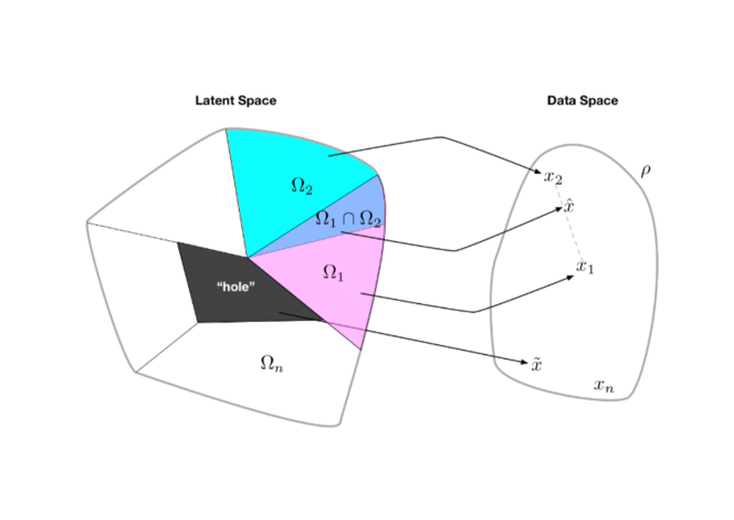
Another striking conclusion we can derive from Propositions 1 and 3 is that the support of the optimal decoder as a function of the latent vector will be concentrated in the support of the marginal posterior. In fact, if we revisit the proof of Proposition 1 in Section C.1 when there are regions in the latent space where we notice that the decoder is completely unconstrained by the ELBO in these regions. We refer to this as the "holes problem" in VAEs. This problem is commonly encountered when using simple Gaussian posteriors (e.g. Kingma2016ImprovedVI ).
3.2 High-capacity -VAEs and spectral methods
The -coefficient in a -VAE Higgins2016vaeLB can be interpreted as the Lagrange multiplier of an inequality constraint imposing either a restriction on the value of the KL-term or a constraint on the reconstruction error Burgess2018UnderstandingDI ; Alemi2017FixingAB . When using the reconstruction error constraint in Equation 2, the Lagrange multiplier is related to the from Higgins2016vaeLB by .
While VAEs with simple linear decoders can be related to a form of robust PCA, Dai2017HiddenTO , we demonstrate a relation between -VAEs with high-capacity decoders and kernel methods such as spectral clustering. More precisely, we show in Proposition 4 that the fixed-point equations of a high-capacity decoder expressed in a particular orthogonal basis are analogous to the reconstruction fixed point equations used in spectral clustering.
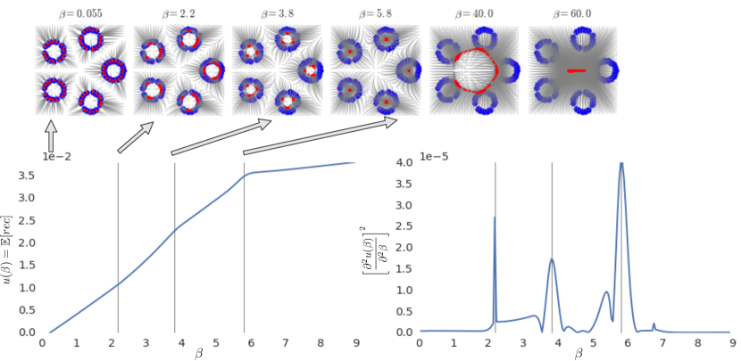
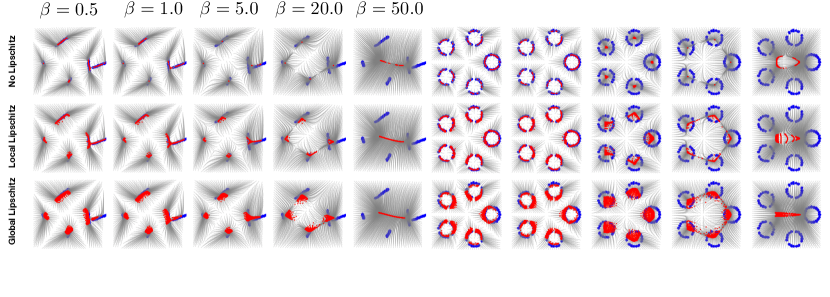
In the literature of spectral clustering and kernel PCA it is known that reconstructions based on a Gaussian Gram matrix may suffer phase-transitions (sudden change in eigen-values or reconstruction fixed-points) as a function of the scale parameter hoyle2004limiting ; nadler2008diffusion ; wang2012kernel ; scholkopf1997kernel ; mika1999kernel . Making a bridge between VAEs and these methods allows us to investigate phase-transitions in high-capacity -VAEs, where the expected reconstruction error is treated as an order parameter . In this case, phase transitions will occur at critical temperature points , which can be detected by analyzing regions of high-curvature (high absolute second-order derivative ). As in spectral clustering, -VAEs phase transitions correspond to the merging of neighboring data-clusters at different spatial scales. This is illustrated in the experiment shown in Figure 2, where we look at the merging of reconstruction fixed-points as we increase . Interestingly, the phase-transitions that we observe are similar to what is known as first-order phase transitions in statistical mechanics blundell2009concepts , but further analysis is necessary to clarify this connection.
Proposition 4.
(High-capacity -VAE and spectral methods) Let be an orthogonal basis in the latent space. If we express the posterior density and generator using this basis respectively as and , where is a matrix with positive entries satisfying the constraint where . The fixed-point equations that maximize the ELBO with respect to are convergent under the appropriate initial conditions and are equivalent to computing the pre-images (reconstructions) of a Kernel-PCA model with a normalized Gaussian Kernel with scale parameter . See proof in Section C.4.
3.3 Equipartition of energy in -VAEs
In statistical mechanics there is an important result, known as equipartition of energy theorem. It states that, for a system in thermodynamic equilibrium, energy is shared equally amongst all accessible degrees of freedom at a fixed energy level, tolman1938principles . We demonstrate that a similar theorem holds for VAEs in Proposition 5. In Proposition 2 we have seen that the optimal posterior for each data point in a high-capacity VAE has its support in the elements of a partition of the latent space and that this partition is equiprobable under the prior. We can generalize this result to -VAEs by noticing that, as a result of the existence of reconstruction fixed points from Proposition 4, there will be regions in the latent space where the Hamiltonian is approximately constant for a given . At these regions, the posterior will be proportional to the prior and they will work as a discrete partition of the latent space, as in Proposition 2. The concept that VAE encoders learn a tiling of the latent space, each tile corresponding to a different level of the function , can be a guiding principle to evaluate generative models as well as to construct more meaningful constraints.
Proposition 5.
(Equipartition of Energy for high-capacity VAEs). Let be the "Hamiltonian" function from Proposition 1 for a VAE trained in a dataset with data-points. For a given data-point , latent point and precision , let . That is, is the set of latent points where the Hamiltonian is approximately constant. As we vary and , each set will be one element of a discrete set of disjoint sets, which we enumerate as . The encoder density will converge to a mixture of the restrictions of the prior to the basis elements . Moreover, the probability of a sample from the prior falling in the partition element is a solution of where is the value of for . See proof in Section C.6.
3.4 The GECO algorithm for VAEs
To derive GECO we start from the augmented Lagrangian defined in Equation 2 for a VAE with decoder parametrized by a vector and an encoder density parametrized by a vector . Optimization of the loss involves joint minimization w.r.t. and , and maximization w.r.t. to the Lagrange multipliers . The parameters and are optimized by directly following the negative gradients of Equation 2. The Lagrange multipliers are optimized following a moving average of the constraint vector . In order to avoid backpropagation through the moving averages, we only apply the gradients to the last step of the moving average. This procedure is detailed in Algorithm 1.
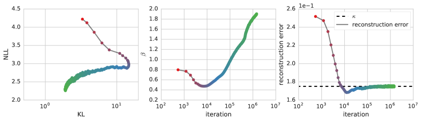
Figure 3 captures a representative example of the typical behavior of GECO: early on in the optimization the solver quickly moves the model parameters into a regime of valid solutions, i.e. parameter configurations satisfying the constraints, and then minimizes ELBO while preserving the validity of the current solution. We refer the reader to Figure 3’s caption for a more detailed description of the optimization phases.
The main advantage of GECO for the machine learning practitioner is that the process of tuning the loss involves the definition of a set of constraints, which typically have a direct relation to the desired model performance, and can be set in the model output space. This is clearly a very different work-flow compared to tweaking abstract hyper-parameters which implicitly affect the model performance. For example, if we were to work in the -VAE setting, we would observe this transition: , where is the reconstruction error constraint as defined in Table 1, and is a tolerance hyper-parameter. On the lhs is an hyper parameter tuning the relative weight of the negative log-likelihood (NLL) and KL terms, affecting model reconstructions in a non-smooth way as shown in Figure 2 and, as discussed in Section 3.2, implicitly defining a constraint on the VAE reconstruction error. On the rhs is a Lagrange multiplier, whose final value is automatically tuned during optimization as a function of the tolerance hyper-parameter, which the user can define in pixel space explicitly specifying the required reconstruction performance of the model.
4 Experiments
4.1 Constrained optimization for large scale models and larger datasets
We demonstrate empirically that GECO provides an easy and robust way of balancing compression versus different types of reconstruction. We conduct experiments using standard implementations of ConvDraw Gregor2016TowardsCC (both in the conditional and unconditional case) and a VAE+NVP model that uses a convolutional decoder similar to Rosca2018DistributionMI and a fully connected conditional NVP dinh2016density model as the encoder density so that we can approximate high-capacity encoders.
In Table 1 we show a few examples of reconstruction constraints that we have considered in this study. To inspect the performance of GECO we look specifically at the behavior of trained models in the information plane (negative reconstruction likelihood vs KL) on various datasets, with and without the RE constraint. All models were trained using Adam kingma2014adam , with learning rate of 1e-5 for ConvDraw and 1e-6 for the VAE+NVP, and a constraint moving average parameter .
| Name | |
|---|---|
| Reconstruction Error (RE) | |
| Feature Reconstruction Error (FRE) | |
| Classification accuracy (CLA) | |
| Patch Normalized Cross-correlation (pNCC) |
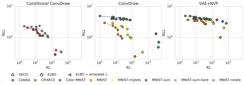
Here we look at the behavior of VAE+NVP and ConvDraw (the latter both in the conditional and unconditional case) in information plane (negative reconstruction likelihood vs KL) on various datasets, with and without a RE constraint.
The datasets we use for the unconditional case are CelebAliu2015faceattributes , Cifar10krizhevsky2009learning , MNISTlecun2010mnist , Color-MNISTunrolledgan and a variant of MNIST we will refer to as MNIST-triplets. MNIST-triplets is comprised of triplets of MNIST digits such that ; the model is trained to capture the joint distribution of the image vectors .
In the conditional case we use are variants of MNIST we will refer to as MNIST-sum, MNIST-sum-hard and MNIST-rotate. All variants of the datasets are comprised of contexts and targets derived from triplets of MNIST digits , with constraints as follows. For MNIST-sum contexts are and targets are , such that ; for MNIST-sum-hard contexts are and targets are , such that ; finally, for MNIST-rotate contexts are and targets are , such that and is rotated about its centre by , note that whilst and have the same label, they are not the same digit instance.
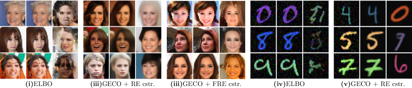
In figure Figure 4 we show in all cases that the negative reconstruction log-likelihoods (NLL, see Appendix D for details) reached by VAE+NVP, ConvDraw and conditional ConvDraw trained only with the ELBO objective are lower compared to the values obtained with ELBO + GECO, at the expense of KL-divergences that are some times many orders of magnitude higher. This result comes from the observation that the numerical values of reconstruction errors necessary to achieve good reconstructions can be much larger, allowing the model to achieve lower compression rates. To provide a notion of the quality of the reconstructions when using GECO, we show in Figure 6 a few model samples and reconstructions for different reconstruction thresholds and constraints. In Appendix F we show reconstructions and samples for all levels of reconstruction targets. As we can see from Figure 6, the use of different constraints has a dramatic impact on both the quality of reconstructions and samples.
4.1.1 Average and Marginal KL analysis
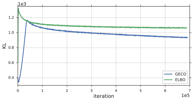
At a fixed reconstruction error, a computationally cheap indicator of the quality of the learned encoder is the average KL between prior and posterior, , which we analyze in Figure 5. Our analysis shows that an expressive model can achieve lower average KL at a given reconstruction error when trained with GECO compared to the same model trained with ELBO.
From Propositions 2 and 5, the optimal solutions for VAE’s encoders are inference models that cover the latent space in such a way that their marginal is equal to the prior. That is, . We refer to the KL between and as the "marginal KL".
If the learned encoder or inference network fails to cover the latent space, it may result in the "holes" problem which, in turn, is associated with bad sample quality.
In contrast to the average KL, the marginal KL is also sensitive to the "holes problem" discussed in Section 1. In Table 2 we evaluate the effect of GECO on the marginal KL of the VAE+NVP models trained in Section 4.1 (in a limited number of combinations due to the significant computational costs) and observe that models trained with GECO also have much lower marginal KL while maintaining an acceptable reconstruction accuracy.
| Dataset | Marginal KL for ELBO | Marginal KL for GECO |
|---|---|---|
| Cifar10 | 725.2 | 45.3 |
| Color-MNIST | 182.5 | 10.3 |
5 Discussion
We have provided a detailed theoretical analysis of the behavior of high-capacity VAEs and variants of -VAEs. We have made connections between VAEs, spectral clustering methods and statistical mechanics (phase transitions). Our analysis provides novel insights to the two most common problems with VAEs: blurred reconstructions/samples, and the "holes problem". Finally, we have introduced GECO, a simple-to-use algorithm for constrained optimization of VAEs. Our experiments indicate that it is a highly effective tool to achieve a good balance between reconstructions and compression in practice (without recurring to large parameter sweeps) in a broad variety of tasks.
Acknowledgements
We would like to thank Mihaela Rosca for the many useful discussions and the help with the Marginal KL evaluation experiments.
References
- [1] Diederik P. Kingma and Max Welling. Auto-encoding variational bayes. CoRR, abs/1312.6114, 2013.
- [2] Danilo Jimenez Rezende, Shakir Mohamed, and Daan Wierstra. Stochastic backpropagation and approximate inference in deep generative models. In ICML, 2014.
- [3] Diederik P. Kingma, Tim Salimans, and Max Welling. Improved variational inference with inverse autoregressive flow. 2016.
- [4] Casper Kaae Sonderby, Tapani Raiko, Lars Maaloe, Soren Kaae Sonderby, and Ole Winther. Ladder variational autoencoders. In NIPS, 2016.
- [5] Karol Gregor, Frederic Besse, Danilo Jimenez Rezende, Ivo Danihelka, and Daan Wierstra. Towards conceptual compression. In NIPS, 2016.
- [6] Ishaan Gulrajani, Kundan Kumar, Faruk Ahmed, Adrien Ali Taiga, Francesco Visin, David Vázquez, and Aaron C. Courville. Pixelvae: A latent variable model for natural images. CoRR, abs/1611.05013, 2016.
- [7] Philip Bachman. An architecture for deep, hierarchical generative models. In NIPS, 2016.
- [8] Kei Akuzawa, Yusuke Iwasawa, and Yutaka Matsuo. Expressive speech synthesis via modeling expressions with variational autoencoder. arXiv preprint arXiv:1804.02135, 2018.
- [9] Wei-Ning Hsu, Yu Zhang, and James Glass. Learning latent representations for speech generation and transformation. arXiv preprint arXiv:1704.04222, 2017.
- [10] Rafael Gómez-Bombarelli, Jennifer N Wei, David Duvenaud, José Miguel Hernández-Lobato, Benjamín Sánchez-Lengeling, Dennis Sheberla, Jorge Aguilera-Iparraguirre, Timothy D Hirzel, Ryan P Adams, and Alán Aspuru-Guzik. Automatic chemical design using a data-driven continuous representation of molecules. ACS Central Science, 2016.
- [11] Mohammad M Sultan, Hannah K Wayment-Steele, and Vijay S Pande. Transferable neural networks for enhanced sampling of protein dynamics. arXiv preprint arXiv:1801.00636, 2018.
- [12] Carlos X Hernández, Hannah K Wayment-Steele, Mohammad M Sultan, Brooke E Husic, and Vijay S Pande. Variational encoding of complex dynamics. arXiv preprint arXiv:1711.08576, 2017.
- [13] Tadanobu Inoue, Subhajit Chaudhury, Giovanni De Magistris, and Sakyasingha Dasgupta. Transfer learning from synthetic to real images using variational autoencoders for robotic applications. arXiv preprint arXiv:1709.06762, 2017.
- [14] Daehyung Park, Yuuna Hoshi, and Charles C Kemp. A multimodal anomaly detector for robot-assisted feeding using an lstm-based variational autoencoder. IEEE Robotics and Automation Letters, 3(3):1544–1551, 2018.
- [15] Herke van Hoof, Nutan Chen, Maximilian Karl, Patrick van der Smagt, and Jan Peters. Stable reinforcement learning with autoencoders for tactile and visual data. In Intelligent Robots and Systems (IROS), 2016 IEEE/RSJ International Conference on, pages 3928–3934. IEEE, 2016.
- [16] SM Ali Eslami, Danilo Jimenez Rezende, Frederic Besse, Fabio Viola, Ari S Morcos, Marta Garnelo, Avraham Ruderman, Andrei A Rusu, Ivo Danihelka, Karol Gregor, et al. Neural scene representation and rendering. Science, 360(6394):1204–1210, 2018.
- [17] Danilo Jimenez Rezende, SM Ali Eslami, Shakir Mohamed, Peter Battaglia, Max Jaderberg, and Nicolas Heess. Unsupervised learning of 3d structure from images. In Advances In Neural Information Processing Systems, pages 4996–5004, 2016.
- [18] SM Ali Eslami, Nicolas Heess, Theophane Weber, Yuval Tassa, David Szepesvari, Geoffrey E Hinton, et al. Attend, infer, repeat: Fast scene understanding with generative models. In Advances in Neural Information Processing Systems, pages 3225–3233, 2016.
- [19] Jakub M. Tomczak and Max Welling. Vae with a vampprior. In AISTATS, 2018.
- [20] Yuri Burda, Roger B. Grosse, and Ruslan Salakhutdinov. Importance weighted autoencoders. CoRR, abs/1509.00519, 2015.
- [21] Eric T. Nalisnick, Lars Hertel, and Padhraic Smyth. Approximate inference for deep latent gaussian mixtures. 2016.
- [22] Danilo Jimenez Rezende and Shakir Mohamed. Variational inference with normalizing flows. In ICML, 2015.
- [23] Tim Salimans, Diederik P. Kingma, and Max Welling. Markov chain monte carlo and variational inference: Bridging the gap. In ICML, 2015.
- [24] Jakub M. Tomczak and Max Welling. Improving variational auto-encoders using householder flow. CoRR, abs/1611.09630, 2016.
- [25] Dustin Tran, Rajesh Ranganath, and David M. Blei. The variational gaussian process. 2015.
- [26] Rianne van den Berg, Leonard Hasenclever, Jakub M. Tomczak, and Max Welling. Sylvester normalizing flows for variational inference. CoRR, abs/1803.05649, 2018.
- [27] Chris Cremer, Xuechen Li, and David K. Duvenaud. Inference suboptimality in variational autoencoders. CoRR, abs/1801.03558, 2018.
- [28] Mihaela Rosca, Balaji Lakshminarayanan, and Shakir Mohamed. Distribution matching in variational inference. CoRR, abs/1802.06847, 2018.
- [29] Lucas Theis, Aäron van den Oord, and Matthias Bethge. A note on the evaluation of generative models. arXiv preprint arXiv:1511.01844, 2015.
- [30] Irina Higgins, Loic Matthey, Arka Pal, Christopher Burgess, Xavier Glorot, Matthew M Botvinick, Shakir Mohamed, and Alexander Lerchner. b-vae: Learning basic visual concepts with a constrained variational framework. 2016.
- [31] Alexander A. Alemi, Ben Poole, Ian Fischer, Joshua V. Dillon, Rif A. Saurous, and Kevin Murphy. Fixing a broken elbo. 2017.
- [32] Naftali Tishby, Fernando C Pereira, and William Bialek. The information bottleneck method. arXiv preprint physics/0004057, 2000.
- [33] Naftali Tishby and Noga Zaslavsky. Deep learning and the information bottleneck principle. In Information Theory Workshop (ITW), 2015 IEEE, pages 1–5. IEEE, 2015.
- [34] Christopher Burgess, Irina Higgins, Arka Pal, Loic Matthey, Nick Watters, Guillaume Desjardins, and Alexander Lerchner. Understanding disentangling in beta-vae. 2018.
- [35] Alexander A. Alemi, Ian Fischer, Joshua V. Dillon, and Kevin P Murphy. Deep variational information bottleneck. CoRR, abs/1612.00410, 2016.
- [36] Shengjia Zhao, Jiaming Song, and Stefano Ermon. Towards deeper understanding of variational autoencoding models. arXiv preprint arXiv:1702.08658, 2017.
- [37] DJ Strouse and David J Schwab. The information bottleneck and geometric clustering. arXiv preprint arXiv:1712.09657, 2017.
- [38] Bin Dai, Yu Wang, John Aston, Gang Hua, and David O Wipf. Hidden talents of the variational autoencoder. 2017.
- [39] I-J Wang and James C Spall. Stochastic optimization with inequality constraints using simultaneous perturbations and penalty functions. In Decision and Control, 2003. Proceedings. 42nd IEEE Conference on, volume 4, pages 3808–3813. IEEE, 2003.
- [40] Ana Maria AC Rocha and Edite MGP Fernandes. A stochastic augmented lagrangian equality constrained-based algorithm for global optimization. In AIP Conference Proceedings, volume 1281, pages 967–970. AIP, 2010.
- [41] Mary Phuong, Max Welling, Nate Kushman, Ryota Tomioka, and Sebastian Nowozin. The mutual autoencoder: Controlling information in latent code representations, 2018.
- [42] Yan Zhang, Mete Ozay, Zhun Sun, and Takayuki Okatani. Information potential auto-encoders. CoRR, abs/1706.04635, 2017.
- [43] Artemy Kolchinsky, Brendan D. Tracey, and David H. Wolpert. Nonlinear information bottleneck. CoRR, abs/1705.02436, 2017.
- [44] Diederik P Kingma and Prafulla Dhariwal. Glow: Generative flow with invertible 1x1 convolutions. arXiv preprint arXiv:1807.03039, 2018.
- [45] Dimitri P. Bertsekas. Constrained Optimization and Lagrange Multiplier Methods (Optimization and Neural Computation Series). 1996.
- [46] Richard Blahut. Computation of channel capacity and rate-distortion functions. IEEE transactions on Information Theory, 18(4):460–473, 1972.
- [47] Imre Csiszár. Information geometry and alternating minimization procedures. Statistics and decisions, 1984.
- [48] Thomas M Cover and Joy A Thomas. Elements of information theory. John Wiley & Sons, 2012.
- [49] Pierre-Alexandre Mattei and Jes Frellsen. Leveraging the exact likelihood of deep latent variable models. CoRR, abs/1802.04826, 2018.
- [50] Sebastian Nowozin, Botond Cseke, and Ryota Tomioka. f-gan: Training generative neural samplers using variational divergence minimization. In Advances in Neural Information Processing Systems, pages 271–279, 2016.
- [51] David Hoyle and Magnus Rattray. Limiting form of the sample covariance eigenspectrum in pca and kernel pca. In Advances in Neural Information Processing Systems, pages 1181–1188, 2004.
- [52] Boaz Nadler, Stephane Lafon, Ronald Coifman, and Ioannis G Kevrekidis. Diffusion maps-a probabilistic interpretation for spectral embedding and clustering algorithms. In Principal manifolds for data visualization and dimension reduction, pages 238–260. Springer, 2008.
- [53] Quan Wang. Kernel principal component analysis and its applications in face recognition and active shape models. arXiv preprint arXiv:1207.3538, 2012.
- [54] Bernhard Schölkopf, Alexander Smola, and Klaus-Robert Müller. Kernel principal component analysis. In International Conference on Artificial Neural Networks, pages 583–588. Springer, 1997.
- [55] Sebastian Mika, Bernhard Schölkopf, Alex J Smola, Klaus-Robert Müller, Matthias Scholz, and Gunnar Rätsch. Kernel pca and de-noising in feature spaces. In Advances in neural information processing systems, pages 536–542, 1999.
- [56] Stephen J Blundell and Katherine M Blundell. Concepts in thermal physics. OUP Oxford, 2009.
- [57] Richard Chace Tolman. The principles of statistical mechanics. Courier Corporation, 1938.
- [58] Laurent Dinh, Jascha Sohl-Dickstein, and Samy Bengio. Density estimation using real nvp. arXiv preprint arXiv:1605.08803, 2016.
- [59] Diederik P Kingma and Jimmy Ba. Adam: A method for stochastic optimization. arXiv preprint arXiv:1412.6980, 2014.
- [60] Ziwei Liu, Ping Luo, Xiaogang Wang, and Xiaoou Tang. Deep learning face attributes in the wild. In Proceedings of International Conference on Computer Vision (ICCV), 2015.
- [61] Alex Krizhevsky and Geoffrey Hinton. Learning multiple layers of features from tiny images. 2009.
- [62] Yann LeCun, Corinna Cortes, and CJ Burges. Mnist handwritten digit database. AT&T Labs [Online]. Available: http://yann. lecun. com/exdb/mnist, 2, 2010.
- [63] Luke Metz, Ben Poole, David Pfau, and Jascha Sohl-Dickstein. Unrolled generative adversarial networks. In ICLR, 2017.
- [64] Mícheál O’Searcoid. Metric spaces. Springer Science & Business Media, 2006.
- [65] Maxwell Rosenlicht. Introduction to analysis. Courier Corporation, 1968.
Appendix A Reconstruction fixed-points experiment details
To produce the results in Figure 2, we iterated the fixed-point equations for the matrix using exponential smoothing with . For each experiment, we iterated the smoothed fixed-point equations until either the number of iterations exceeded 400 steps or the Euclidean distance between two successive steps became smaller than 1e-3. The basis functions were arranged as a 32x32 grid in a compact latent space , the prior was chosen to be uniform, . The matrix was initialized at the center-points of the grid tiles with small uniform noise in .
Appendix B High-capacity -VAEs and Lipschitz constraints
The analysis of high-capacity VAEs in Sections 3.1 and 3.2 reveal interesting aspects of VAEs near convergence, but the type of solutions implied by Propositions 2 and 4 may seem unrealistic for VAEs with smooth decoders parametrized by deep neural networks. For instance, the solutions of the fixed point-equations from Propositions 2 and 4 have no notion that the outputs of the decoder and for two similar latent vectors and should also be similar. That is, these solutions are not sensitive to the metric and topological properties of the latent space. This implies that, if we want to work in a more realistic high-capacity regime, we must further constrain the solutions so that they have at least a continuous limit as we grow the number of basis functions to infinity.
A sufficient condition for a function to be continuous, is that it is a locally-Lipschitz function of [64]. Thus, to bring our analysis closer to more realistic VAEs, we consider high-capacity -VAEs with an extra -Lipschitz inequality constraint in the decoder function . The new term that we add to the augmented Lagrangian, with a functional Lagrange multiplier is given by
| (7) |
By expressing and in the functional basis of Proposition 4, and , we can rewrite the constraint term as a quadratic inequality constraint in the matrix ,
| (8) |
where are new Lagrange multipliers, and . The matrices and embed the metric and topological properties of the latent space but are otherwise independent of the rest of the model.
The constraint (7) can be used to enforce both global and local Lipschitz constraints by controlling the size of the support of the Lagrange multiplier function . If for , we will be constraining the decoder function to be locally Lipschitz within a radius in the latent space.
Note that the Lipschitz constraint is not a reconstruction constraint as it only constrains the VAE’s decoder at arbitrary points in the latent space. For this reason, it can be implemented as a projection step just after the iteration from Equation 20. This is formalized in Proposition 6. We illustrate the combined effect of , local and global Lipschitz constraints on VAEs in Figure 7.
Proposition 6.
The Lipschitz constraint from Equation 8 can be incorporated to the fixed-point Equation 20 as a projection of the form , where is the transition operator without Lipschitz constraints. See proof in Section C.5.
Appendix C Proofs
C.1 Derivation of Proposition 1
Proof.
We can obtain these equations by taking the functional derivatives , , and of and with respect to and respectively and re-arranging the terms of the equations , , and . For the density we must also take the normalization constraint into account:
| (9) | ||||
| (10) | ||||
| (11) | ||||
| (12) |
where was computed using a Gaussian likelihood with global variance . A straightforward algebraic simplification of these equations results in the fixed-point equations of the Proposition 1. For a general constraint we cannot simply solve for due to the non-linear dependency of on . In this case, we can often employ a standard technique for constructing fixed-point equations which consists in converting an equation of the form to a recurrence relation of the form . ∎
C.2 Derivation of Proposition 2
Proof.
First, we note that for any given , the ELBO is a convex quadratic functional of the decoder and, for a fixed , it is a convex functional of the encoder . Second, for a fixed partition , replacing the solution , where , in the fixed-point equations, results in itself. That is,
| (13) | ||||
| (14) | ||||
| (15) | ||||
| (16) |
Therefore, is a fixed-point in the family of densities constrained by the partition . We observe that the negative ELBO reduces to the expected KL term only, . We can now optimize the partition to further maximize the ELBO. This results in . That is, the tiles must be equiprobable. At this point, we have . ∎
C.3 Derivation of Proposition 3
Proof.
C.4 Derivation of Proposition 4
Proof.
The expression for the generator can be obtained by substitution and algebraic simplification using the fact that form an orthogonal basis and that :
| (18) |
with . Similarly, we can compute the fixed point equations for by substitution on equations (5) and (6),
| (19) | ||||
| (20) |
where and . If the initial reconstruction vectors are in the convex-hull of the training data-points, then equations (20) will map them to another set of points in the convex-hull of the training data. Since, these equations are also smooth with respect to , they are guaranteed to converge as a consequence of the fixed-point theorem [65]. Importantly, equation (20) corresponds to the fixed point iterations for computing the pre-image (reconstructions) of Kernel-PCA but using a normalized Gaussian kernel. ∎
C.5 Derivation of Proposition 6
Proof.
We first write the relevant terms of the augmented Lagrangian in the basis from Proposition 4,
| (21) | ||||
| (22) | ||||
| (23) |
where cst are terms that do not depend on for a fixed . Solving with respect to results in
| (24) | ||||
| (25) |
where ∎
C.6 Derivation of Proposition 5
Proof.
From Proposition 4, we have seen that the reconstruction vectors of a high-capacity -VAE will converge to a set of fixed-points. This means that will map the set basis-functions to a smaller subset of points. As a consequence, all the latent-vectors falling in the support of these basis elements will also map to the same reconstruction and for a fixed , the function will only have possible distinct values, which we can enumerate as . If we enumerate all distinct supports as , then from Equation 5 we have that . Replacing in Equation 2 and maximizing with respect to results in the condition . ∎
Appendix D Computing -independent NLLs
When we train -VAEs with different constraints using GECO, it is not obvious how to compare them in the information plane due to the arbitrary scaling learned by the optimizer. In order to do a more meaningful comparison after the models have been trained, we recompute an optimal global standard-deviation for all models on the training data (keeping all other parameters fixed):
| (26) |
where and and is the batch size used for this computation. All the reported negative reconstruction likelihoods were computed using . We report all likelihoods per-pixel using the "quantized normal" distribution [28] to make it easier to compare with other models.
Appendix E Extra Experiments
E.1 Micro-MNIST
As a way to illustrate the impact of different constraints on the learned encoder densities, we created the "Micro-MNIST" dataset, comprised of only 7 random samples from MNIST. In these experiments, shown in Figure 8, we observed that as we make the constraints weaker (larger for the RE constraint or smaller for the CLA constraint), we encourage the posterior density to collapse the modes of the data, focusing on the properties of the data relevant to the constraints.

Appendix F Model and Data Samples




















