Synchronization of strongly interacting alkali-metal spins

Abstract

The spins of gaseous alkali atoms are commonly assumed to oscillate at a constant hyperfine frequency, which for many years has been used to define the Second. Indeed, under standard experimental conditions, the spins oscillate independently, only weakly perturbed and slowly decaying due to random spin-spin collisions. Here we consider a different, unexplored regime of very dense gas, where collisions, more frequent than the hyperfine frequency, dominate the dynamics. Counter-intuitively, we find that the hyperfine oscillations become significantly longer-lived, and their frequency becomes dependent on the state of the ensemble, manifesting strong nonlinear dynamics. We reveal that the nonlinearity originates from a many-body interaction which synchronizes the electronic spins, driving them into a single collective mode. The conditions for experimental realizations of this regime are outlined.

Binary collisions are a fundamental relaxation mechanism in atomic spin ensembles. During a collision, a pair of atoms within the ensemble briefly interacts, and its mutual electronic wavefunction is altered. Since the impact parameters are random, the quantum state of the ensemble relaxes at a rate $R$, proportional to the collisions rate $\Gamma$ (Happer-book-2010, ). This prevailing relaxation mechanism limits the sensitivity of shot-noise-limited atomic sensors (Kitching-sensors-review, ), such as magnetometers (Romalis-multipass-PRL-2013, ; Polzik-Magnetometery, ), gyroscopes (Romalis-Comagnetometer-gyro, ), accelerometers (Biedermann-warm-vapor-interferometer-2017, ), and clocks (Vanier-atomic-clocks, ; Campero-clocks, ; Kitching-clocks, ; Novikova-LinPerLin-Clock, ; Happer-end-state-clock-2004, ). It is often desirable to increase the density of the ensemble in order to either increase the signal-to-noise ratio or to allow for miniaturization of the device. However with the increased density, the collisional relaxation rate $R\sim\Gamma$ increases, yielding no improvement in the sensor sensitivity (Kitching-sensors-review, ).

Polarized alkali ensembles were shown to overcome this limit at low magnetic fields (happer-SERF-1977, ; Nonlinear-SERF, ; SERF_quantum_information, ). When the Zeeman splitting $\omega_{B}$ satisfies $\omega_{B}\ll\Gamma,$ the magnetic Zeeman coherences undergo a process akin to motional narrowing via frequent spin-exchange collisions. The relaxation rate is reduced to $R\sim\omega_{B}^{2}/\Gamma$ and so is the magnetic linewidth. This effect, denoted as spin-exchange relaxation free (SERF), stimulated the development of SERF magnetometers with unprecedented sensitivities (Budker-Romalis-optical-magnetometery, ).

While SERF protects the Zeeman coherences at high atomic densities, the hyperfine coherences widely used for quantum information applications (Shu_vapor, ; Nunn-Raman, ; Polzik-RMP-2010, ), radio astronomy (21-cm-line, ) and atomic clocks (Vanier-atomic-clocks, ; Campero-clocks, ; Kitching-clocks, ; Novikova-LinPerLin-Clock, ; Happer-end-state-clock-2004, ) are subject to rapid relaxation rates $R\sim\Gamma$. It is therefore widely accepted that increased density yields faster decoherence (happer-SERF-1977, ). In this letter, we prove the opposite. We derive the collisional dynamics of a dense ensemble and find that the hyperfine coherence-time increases significantly at high densities. We further show that rapid spin-exchange collisions synchronize the individual spins to a single frequency, which depends on the collective spin magnitude, leading to a unique nonlinear many-body dynamics.

Consider first a toy model of $N$ alkali atoms, whose ground level encompasses an electronic spin $S=1/2$ and a nuclear spin $I=1/2$. Most standard models describe the spin state and interactions with an effective ensemble-averged set of equations (Schwinger-average-density-matrix, ; Happer-Romalis-SEOP-1998, ; Happer-book-2010, ; happer-SERF-1977, ). Here we generalize these derivations and describe the many-body dynamics of the different atoms using a general master equation formalism of open quantum systems (see SI for the full derivation (supplemnetary-1, )). The atomic state of the $n^{\mbox{th}}$ atom is described by the observables of electronic spin $\mathbf{S}_{n}$, nuclear spin $\mathbf{I}_{n}$, and hyperfine coherence $\mathbf{A}_{n}\equiv\mathbf{S}_{n}\times\mathbf{I}_{n}$. The electrons are internally coupled to their nuclei by the hyperfine interaction $\omega_{n}\mathbf{S}_{n}\cdot\mathbf{I}_{n}$, while every pair of electrons $\mathbf{S}_{n},\mathbf{S}_{m}$ experiences spin-exchange interaction at a time-averaged rate $\Gamma_{mn}$. At time scales longer than the time between collisions $\sim(\sum_{m}\Gamma_{mn})^{-1}$, the coherences between different atoms average to zero due to the randomness of collisions (Happer-book-2010, ). The many-body dynamics of the atoms can then be represented by a compact set of $9N$ nonlinear first-order Bloch equations,

$$\frac{d}{dt}\left\langle\mathbf{S}_{n}\right\rangle\, =\omega_{n}\left\langle\mathbf{A}_{n}\right\rangle+\sum_{m}\Gamma_{mn}\left(\left\langle\mathbf{S}_{m}\right\rangle-\left\langle\mathbf{S}_{n}\right\rangle\right)$$ (1)

$$\frac{d}{dt}\left\langle\mathbf{I}_{n}\right\rangle\, =-\omega_{n}\left\langle\mathbf{A}_{n}\right\rangle$$ (2)

$$\frac{d}{dt}\left\langle\mathbf{A}_{n}\right\rangle =-\frac{\omega_{n}}{2}\left(\left\langle\mathbf{S}_{n}\right\rangle-\left\langle\mathbf{I}_{n}\right\rangle\right)-\sum_{m}\Gamma_{mn}\left\langle\mathbf{A}_{n}\right\rangle$$ (3)

$$+\sum_{m}\Gamma_{mn}\left\langle\mathbf{S}_{m}\right\rangle\times\left\langle\mathbf{I}_{n}\right\rangle.$$

The first term in Eqs. (1-3) describes the hyperfine precession of $\left\langle\mathbf{S}_{n}\right\rangle$ and $\left\langle\mathbf{I}_{n}\right\rangle$ through the coupling with the hyperfine-coherence vector $\left\langle\mathbf{A}_{n}\right\rangle$. The second term in Eq. (1) describes the collisional exchange between the $n^{\mbox{th}}$ electronic spin and all its neighbors. This term tends to synchronize all $\left\langle\mathbf{S}_{n}\right\rangle$ by equilibrating them with the other electronic spins $\left\langle\mathbf{S}_{m}\right\rangle$. In Eq. (3), the second term describes a decay of the hyperfine coherences at a rate $\sum_{m}\Gamma_{mn}$, and the last term describes the nonlinear coherence build-up, a result of the spin-conservative part of the collisional interaction (supplemnetary-1, ).

Spin may be exchanged between atoms when they collide, but their total spin is conserved. Defining the atomic spin operators $\mathbf{F}_{n}=\mathbf{S}_{n}+\mathbf{I}_{n}$, we find from Eqs. (1-3) that the total spin of the ensemble $\left\langle\mathbf{F}\right\rangle\equiv\sum_{n}\left\langle\mathbf{F}_{n}\right\rangle$ is constant,

$$\frac{d}{dt}\left\langle\mathbf{F}\right\rangle\equiv\frac{1}{N}\sum_{n}\frac{d}{dt}\left\langle\mathbf{F}_{n}\right\rangle=0.$$ (4)

In practice, this property holds for time scales shorter than the spin destruction rate of the ensemble (see SI (supplemnetary-1, )). As no external magnetic field is included, the model is isotropic, and the constant $\left\langle\mathbf{F}\right\rangle$ essentially sets a preferred direction.

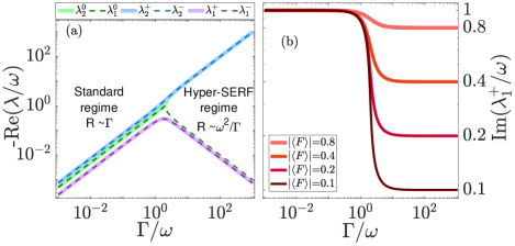
Figure 1: (a) Relaxation rates of the hyperfine coherences for $I=1/2$ and $\left|\left\langle\mathbf{F}\right\rangle\right|=1/2$. At high collision rates $\Gamma\gg\omega$ (high densities), the relaxation of the $\lambda_{1}^{\pm,0}$ modes decreases. (b) Modified hyperfine frequencies. At high collision rates, the oscillation frequency of the hyperfine coherences becomes linearly dependent on the magnitude of the spin $\left|\left\langle\mathbf{F}\right\rangle\right|$.

We first consider the mean-field solution of Eqs. (1-3), assuming that $\omega_{n}\rightarrow\omega$, $\Gamma_{mn}\rightarrow\Gamma/N$, and $\left\langle\mathbf{F}_{n}\right\rangle\rightarrow\left\langle\mathbf{F}\right\rangle$. It follows that ${\color[rgb]{0,0,1}{\color[rgb]{0,0,0}\left\langle\mathbf{S}_{n}\right\rangle=\sum_{n}\left\langle\mathbf{S}_{n}\right\rangle/N}}\equiv\left\langle\mathbf{S}\right\rangle$, satisfying

$$\ddot{\left\langle\mathbf{S}\right\rangle}+\Gamma\dot{\left\langle\mathbf{S}\right\rangle}+\omega^{2}\left(\mathbf{\left\langle S\right\rangle}-\nicefrac{{1}}{{2}}\left\langle\mathbf{F}\right\rangle\right)-\omega\Gamma\mathbf{\left\langle F\right\rangle\times\left\langle S\right\rangle}=0.$$ (5)

Since $\left\langle\mathbf{F}\right\rangle$ is constant, Eq. (5) is a set of three linear non-homogeneous equations, whose general solution is

$$\left\langle S_{q}\right\rangle=\frac{1}{2}\left\langle F_{q}\right\rangle+\sum_{i=1}^{2}a_{i}^{q}e^{-\lambda_{i}^{q}t}.$$

Here, the subscript $q=0,\pm$ denotes the three directions $\hat{z,}\left(\hat{x}\pm i\hat{y}\right)/\sqrt{2}$, with the $\hat{z}$ axis defined as the direction of the vector $\left\langle\mathbf{F}\right\rangle$, and the six coefficients $a_{i}^{q}$ determine the weights of the modes and depend on the initial condition of the spins. The time-dependent dynamics are described by six complex eigenvalues

$$\left(\begin{array}[]{c}\lambda_{1,2}^{0}\\ \lambda_{1,2}^{+}\\ \lambda_{1,2}^{-}\end{array}\right)=\frac{1}{2}\left(\begin{array}[]{c}-\Gamma\pm\sqrt{\Gamma^{2}-4\omega^{2}}\\ -\Gamma\pm\sqrt{\Gamma^{2}+4i\Gamma\omega\left|\left\langle\mathbf{F}\right\rangle\right|-4\omega^{2}}\\ -\Gamma\pm\sqrt{\Gamma^{2}-4i\Gamma\omega\left|\left\langle\mathbf{F}\right\rangle\right|-4\omega^{2}}\end{array}\right),$$ (6)

where $\lambda_{1,2}^{0},$ $\lambda_{1,2}^{+}$, and $\lambda_{1,2}^{-}$ are the eigenvalues of $\left\langle S_{0}\right\rangle$, $\left\langle S_{+}\right\rangle$, and $\left\langle S_{-}\right\rangle$ respectively. The real part of these eigenvalues, associated with the relaxation rate $R$, is shown in Fig. 1(a) for a partially polarized ensemble $\left|\left\langle\mathbf{F}\right\rangle\right|=1/2$.

In standard hot vapor experiments, the alkali densities are kept low, such that $\Gamma\ll\omega$. In this regime, the eigenvalues in (6) are approximately given by

$$\left(\begin{array}[]{c}\lambda_{1,2}^{0}\\ \lambda_{1}^{\pm}\\ \lambda_{2}^{\pm}\end{array}\right)\approx\left(\begin{array}[]{c}\pm i\omega-\Gamma/2\\ \pm i\omega-\left(1-\left|\left\langle\mathbf{F}\right\rangle\right|\right)\Gamma/2\\ \pm i\omega-\left(1+\left|\left\langle\mathbf{F}\right\rangle\right|\right)\Gamma/2\end{array}\right).$$ (7)

The oscillation frequency of the hyperfine coherences $\left|\mbox{Im}\left(\lambda\right)\right|=\omega$ is constant. The relaxation rate of the $\lambda_{1,2}^{0}$ modes, associated with the so-called clock transition ($0-0$) used by atomic frequency standards (Vanier-atomic-clocks, ; Kitching-clocks, ; Novikova-LinPerLin-Clock, ), is $R=\Gamma/2$. The end resonances relax at $R=\left(1-\left|\left\langle\mathbf{F}\right\rangle\right|\right)\Gamma/2$, leading to the well-known line narrowing for $\left|\left\langle\mathbf{F}\right\rangle\right|\rightarrow 1$ (Happer-end-state-clock-2004, ).

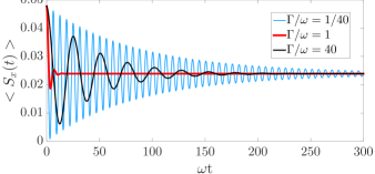
Figure 2: Numerical simulation of the mean-field case. The coherence time revives at high densities $\Gamma\gg\omega$.

In the strong interaction regime $\Gamma\gg\omega$, the hyperfine oscillation is strongly perturbed by spin-exchange collisions, and the eigenvalues in (6) become

$$\left(\begin{array}[]{c}\lambda_{2}^{0}\\ \lambda_{1}^{0}\\ \lambda_{2}^{\pm}\\ \lambda_{1}^{\pm}\end{array}\right)\approx\left(\begin{array}[]{c}-\Gamma\\ -\omega^{2}/\Gamma\\ \pm i\omega\left|\left\langle\mathbf{F}\right\rangle\right|-\Gamma\\ \pm i\omega\left|\left\langle\mathbf{F}\right\rangle\right|-\left(1-\left|\left\langle\mathbf{F}\right\rangle\right|^{2}\right)\omega^{2}/\Gamma\end{array}\right).$$ (8)

We find that the relaxation of the $\lambda_{1}^{\pm,0}$ modes scales as $\omega^{2}/\Gamma$, which we attribute to motional narrowing; increasing the collision rate $\Gamma$ slows down the hyperfine decoherence. We denote this property as hyper-SERF, as the hyperfine coherences become free from spin-exchange relaxation. Furthermore and quite uniquely, the hyperfine frequency becomes dependent on the absolute magnitude of the spin $\left|\left\langle\mathbf{F}\right\rangle\right|$. The modified frequency of the $\lambda_{1,2}^{\pm}$ modes, shown in Fig. 1(b), is given by $\omega\left|\left\langle\mathbf{F}\right\rangle\right|$. On the other hand, the $\lambda_{1,2}^{0}$ modes have no oscillatory terms, indicating that the $0-0$ clock-transition will “stop ticking”.

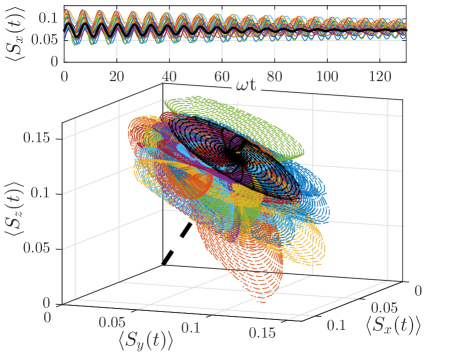
Figure 3: Precession of the electronic spins in the standard, low density regime with $\Gamma=\omega/100$ (25 out of N=100 simulated spins are shown). Each electronic spin $\left\langle\mathbf{S}_{n}\right\rangle$ precesses independently around its local vector $\left\langle\mathbf{F}_{n}\right\rangle$, slowly decaying due to collisions. The mean electronic spin (black) precesses around the conserved spin $\left\langle\mathbf{F}\right\rangle$ (black dotted line), dephasing at an increased rate $R\sim\mbox{max}\left(\Gamma,\Delta\omega\right)$.

To understand the nature of this mechanism, we generalize the mean-field result by numerically solving Eqs. (1-3) and obtaining the many-body dynamics of the spins. The initial values of $\left\langle\mathbf{S}_{n}\right\rangle,\left\langle\mathbf{I}_{n}\right\rangle,\left\langle\mathbf{A}_{n}\right\rangle$ are derived from the initial density matrices of the atoms $\rho_{n}$. We start with an optically pumped vapor in a spin-temperature distribution $\tilde{\rho}_{n}=\mbox{exp}(-\beta F_{n}^{z})/Z$, where $0\leq\beta\leq 1$ determines the degree of polarization, and $Z$ is a normalization factor (Happer-Romalis-SEOP-1998, ). To generate initial hyperfine coherences, we perturb $\tilde{\rho}_{n}$ by tilting the electronic spins by angles $\theta_{n}^{y},\theta_{n}^{z}$ and the nuclear spins by angles $\phi_{n}^{y},\phi_{n}^{z}$, such that $\rho_{n}=U_{n}\tilde{\rho}_{n}U_{n}^{\dagger}$ with the rotation matrices

$$U_{n}=e^{i\theta_{n}^{z}S_{z}}e^{i\theta_{n}^{y}S_{y}}e^{i\phi_{n}^{z}I_{z}}e^{i\phi_{n}^{y}I_{y}}.$$

We first simulate the mean-field solution for $N=100$, $\omega_{n}=\omega$, and $\Gamma_{mn}=\Gamma/N$, as shown in Fig. 2. The initial conditions are given by $\theta_{n}^{z}=\phi_{n}^{y}=\phi_{n}^{z}=0$, $\theta_{n}^{y}=\pi/8$ and $\beta=0.51$ ($\left|\left\langle\mathbf{F}\right\rangle\right|=\nicefrac{{1}}{{4}}$). We find indeed that the coherence time of the mean spin $\left\langle S_{x}\right\rangle$ is improved at high collision rate $\Gamma$. We further simulate the many-body dynamics of the spins for unequal initial values and unequal interaction strengths $\omega_{n}$ and $\Gamma_{mn}$. We set $\beta=0.73$ ($\left|\left\langle F\right\rangle\right|=0.32$), $\theta_{n}^{y},\theta_{n}^{z}$$\sim\mathcal{N}\left(\nicefrac{{\pi}}{{3}},\nicefrac{{\pi}}{{15}}\right)$ ,$\phi_{n}^{y},\phi_{n}^{z}\sim\mathcal{N}\left(\nicefrac{{\pi}}{{6}},\nicefrac{{\pi}}{{30}}\right)$, randomly sampled from a normal distribution $\mathcal{N}\left(\mu,\sigma\right)$ with mean $\mu$ and standard deviation $\sigma$, resulting with unequal initial spin orientations. The collision rates $\Gamma_{mn}=\Gamma p_{mn}$ are set by generating a random double stochastic matrix $p_{mn}$. For the generality of the model, we also allow a spread for the atomic hyperfine frequencies $\omega_{n}\sim\mathcal{N}\left(\omega,\omega/50\right)$. In the standard, low density, regime ($\Gamma\ll\omega_{n}$), the individual electronic spins preces independently at their inherent frequencies $\omega_{n}$, forming spiral trajectories around their local spin vectors $\left\langle\mathbf{F}_{n}\right\rangle$, as shown in Fig. 3. The local spin vectors slowly relax to their equilibrium state $\left\langle\mathbf{F}_{n}\right\rangle\rightarrow\left\langle\mathbf{F}\right\rangle=\frac{1}{N}\sum_{n}\left\langle\mathbf{F}_{n}\right\rangle$ due to spin-exchange collisions, at a rate $R\sim\Gamma/2$. As a result, the spin coherences decay, and the center of each spiral adiabatically follows $\left\langle\mathbf{F}_{n}\right\rangle$. The mean electronic spin $\frac{1}{N}\sum_{n}\left\langle S_{x}^{n}\right\rangle$ (black line in Fig. 3), decays faster than the individual spins $\left\langle S_{x}^{n}\right\rangle$. This results from an additional (inhomogeneous) dephasing of the different hyperfine frequencies $\omega_{n}$ with a relaxation rate $R\sim[\sum_{n}(\omega_{n}-\omega)^{2}]^{1/2}\equiv\Delta\omega$.

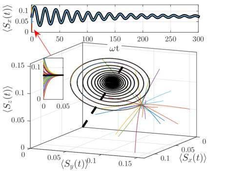
Figure 4: Synchronization of the electronic spins in the strong interaction regime with $\Gamma=100\omega$ (25 out of N=100 simulated spins are shown). The electronic spins synchronize rapidly after $t\sim\Gamma^{-1}$ to a common electronic mode (black). The electronic spins precess coherently at a modified, spin-dependent, frequency $\Omega$ and decay at a slow rate $R\sim\omega^{2}/\Gamma$.

In the strong interaction regime ($\Gamma\gg\omega$), the electronic spins no longer precess individually, but rather synchronize to a single trajectory as shown in Fig. 4. All spins precesses around the mean spin $\left\langle\mathbf{F}\right\rangle$ with identical frequency of oscillation $\Omega$. The synchronization time is rapid, scaling as $\Gamma^{-1}$. To reveal the synchronization mechanism, we expand Eqs. (1-3) by the small parameter $\omega/\Gamma$, keeping only second order terms (supplemnetary-1, ),

$$\frac{d}{dt}\left\langle\mathbf{F}_{n}\right\rangle =\sum_{m}\Gamma_{mn}\left(\left\langle\mathbf{S}_{m}\right\rangle-\left\langle\mathbf{S}_{n}\right\rangle\right)$$ (9)

$$\frac{d}{dt}\left\langle\mathbf{S}_{n}\right\rangle \approx\sum_{m}\Gamma_{mn}\left(\left\langle\mathbf{S}_{m}\right\rangle-\left\langle\mathbf{S}_{n}\right\rangle\right)+\omega_{n}\left\langle\mathbf{F}_{n}\right\rangle\times\left\langle\mathbf{S}_{n}\right\rangle$$

$$- \frac{\omega_{n}^{2}}{\Gamma_{n}}\left(\left\langle\mathbf{S}_{n}\right\rangle-\nicefrac{{1}}{{2}}\left\langle\mathbf{F}_{n}\right\rangle\right)$$ (10)

This set of equations is known as the “tops model” (Ritort-Tops-Model-1998, ), with $\omega_{n}\left\langle\mathbf{F}_{n}\right\rangle$ playing the role of a local external torque. The first term in Eq. (10) initially dominates and synchronizes the electronic spins over a transient time $\sim\Gamma^{-1}$, as shown in Fig. 4. Once the electronic spins are synchronized $\left\langle\mathbf{S}_{m}\left(t\right)\right\rangle\approx\left\langle\mathbf{S}_{n}\left(t\right)\right\rangle$, the spin vectors $\left\langle\mathbf{F}_{n}\right\rangle$ remain approximately constant [Eq. (9)]. The second term in Eq. (10) describes a local torque exerted on $\left\langle\mathbf{S}_{n}\right\rangle$ by the local field $\omega_{n}\left\langle\mathbf{F}_{n}\right\rangle$. We note that the directions and magnitudes of these local fields could be random. The third and least dominant term in Eq. (10) describes the slow relaxation of the electronic spin $\left\langle\mathbf{S}_{n}\right\rangle$ towards its steady value $\left\langle\mathbf{F}_{n}\right\rangle/2$ at the hyper-SERF rate $\omega_{n}^{2}/\Gamma_{n}$. It is interesting to note that, although the electronic spins are frustrated by the different local fields $\omega_{n}\left\langle\mathbf{F}_{n}\right\rangle,$ the synchronization term overcomes this frustration in the strong-interaction regime. As a result, the synchronized electronic spins precess collectively around an effective mean field

$$\mathbf{\boldsymbol{\Omega}}\approx\frac{1}{N}\sum_{n}\omega_{n}\left\langle\mathbf{F}_{n}\right\rangle.$$ (11)

Hence electronic spins with random initial orientations are phase-synchronized, and consequently precess coherently around the vector $\boldsymbol{\mathbf{\Omega}}$, with a new collective modified hyperfine frequency $\Omega$. Note that our result are valid also for the case of nonequal frequencies $\omega_{n}$. This frequency depends on the polarization of the spin vectors $\left\langle\mathbf{F}_{n}\right\rangle$, recovering the mean-field results when $\omega_{n}=\omega$. Since the vectors $\left\langle\mathbf{F}_{n}\right\rangle$ do not synchronize, the directions of the nuclear spins $\left\langle\mathbf{I}_{n}\right\rangle$ remain unsynchronized as well. Nevertheless, the different nuclear spins precess coherently, experiencing the slow electronic relaxation $\omega_{n}^{2}/\Gamma_{n}$.

It is also instructive to interpret our results from the viewpoint of collision-driven thermal equilibration, by extending the description of the SERF effect in Ref. (happer-SERF-1977, ) and considering the hyperfine interaction as an out-of-equilibrium term. At low atomic densities, spin-exchange collisions reduce the electron-nuclear coherence, as they redistribute the electronic spin between different atoms. At the same time, the hyperfine interaction strongly couples the nuclear spin to the electron spin within each atom. Consequently, the system is driven into a so-called spin-temperature distribution $\rho_{n}=\mbox{exp}(-\vec{\beta}\mathbf{F}_{n})/Z$ with no hyperfine coherence, thus maximizing the entropy of the spin degrees-of-freedom (Anderson-Pipkin, ; spin-temperature2, ). The mean thermalization rates of the different hyperfine coherences correspond to the decay rates of Eq. (7) (proportional to $\Gamma$). In contrast, at high atomic densities, the electron spins alone quickly thermalize (at a rate $\Gamma$) into a spin-temperature distribution $\rho_{n}^{s}=\mbox{exp}(-\vec{\beta}_{s}\mathbf{S}_{n})/Z_{s}$ through the spin-synchronizing term in Eq. (1). This thermalization leads to rapid loss of any initial correlations between the electronic and nuclear spins, making the electronic spins act as a single macroscopic magnetic moment on the nuclear spins $\left\langle\mathbf{A}_{n}\right\rangle\approx\left\langle\mathbf{S}\right\rangle\times\left\langle\mathbf{I}_{n}\right\rangle$. Application of this result to Eq. (1) shows that $|\vec{\beta}_{s}|=2\text{atanh}\left(2\left|\left\langle\mathbf{S}\right\rangle\right|\right)$ is constant in magnitude but precesses according to $\partial_{t}\hat{\beta}_{s}=\hat{\beta}_{s}\times\boldsymbol{\mathbf{\Omega}}$, i.e., the electronic spins oscillate around the modified hyperfine vector $\boldsymbol{\mathbf{\Omega}}$. In turn, the nuclear spins precess around the electronic spin $\left\langle\mathbf{S}\right\rangle$ as suggested by Eq. (2), also with a precession frequency $\mathbf{\Omega}$. Full thermalization of the nuclear spins happens slowly, at an approximate rate $\sim\Gamma\left(\omega/\Gamma\right)^{2}$, where $\left(\omega/\Gamma\right)^{2}$ is the small angular loss during the synchronization time, similar to the loss in standard SERF of the Zeeman coherences (happer-SERF-1977, ).

Our model predicts several new physical phenomena in the strong interaction regime $\Gamma\gg\omega$. The first prediction is the motional narrowing of the hyperfine coherence, leading to its slow relaxation with a rate that scales as $\omega^{2}/\Gamma$ rather than $\Gamma$. The second prediction of the model is the nonlinear splitting of the hyperfine levels, “dressed” by the collisional interaction, such that both electronic and nuclear spins should precess at a rate $\omega\left\langle\left|\boldsymbol{F}\right|\right\rangle$. The splitting depends linearly on the magnitude of the spin, and should therefore vary for different optical-pumping rates. This dependence can thus lead to intriguing nonlinear behavior when the probing scheme inherently involves optical pumping, such as in coherent population trapping (CPT) (cpt, ). A third prediction pertains to the case of nonzero bandwidth $\Delta\omega$. For alkali ensembles, a mixture of different species with different hyperfine frequencies $\omega_{n}$ effectively features nonzero $\Delta\omega$. In these hybrid ensembles, the electronic spins of all species would synchronize and oscillate in a common mode. The synchronization mechanism can be optically probed by measuring the oscillation frequency of each specie separately (Hybrid_spin_exchange, ).

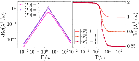
Figure 5: Numerical calculation of hyper-SERF for $I=3/2$, for different initial polarizations $\left|\left\langle\mathbf{F}\right\rangle\right|$. Shown are the dominant relaxation rate of $\left\langle S_{x}\right\rangle$ (left) and its frequency (right). The results are qualitatively similar to the $I=1/2$ case (note that here the maximal spin is $\left|\left\langle\mathbf{F}\right\rangle\right|=2$).

We analyzed above a toy model with $I=1/2$ and no magnetic field ($\vec{B}=0$). To verify that the hyper-SERF features persist for $I>1/2$ we numerically solved the master equation (supplemnetary-1, ). Fig. 5 presents the dominant relaxation rate and frequency of $\left\langle S_{x}\right\rangle$ for atoms with $I=3/2$, initialized with $\theta^{z}=\phi^{y}=\phi^{z}=0$, $\theta^{y}=\pi/8$. These results show that the toy model results are qualitatively valid for $I>1/2$ spins. If a magnetic field is applied, both the direction and magnitude of $\left\langle\mathbf{F}\right\rangle$ could vary in the presence of collisions. At magnetic fields $B\lesssim 10\,\text{Gauss}$, the Zeeman splitting is small $(g_{s}B\ll\omega$, where $g_{s}$ is the gyromagnetic ratio), $\left\langle\mathbf{F}\right\rangle$ slowly precesses around $\vec{B}$, and our solution for the hyperfine coherences adiabatically follows the instantaneous $\left\langle\mathbf{F}\right\rangle$.

Experimental Roadmap. Hyper-SERF with $I=3/2$ can be experimentally realized using ⁴¹K, which has the lowest hyperfine frequency $2\omega_{{\scriptscriptstyle\textsc{{K}}}}\sim 254\,(2\pi)$ MHz (the factor of 2 enters since $I=3/2$). The density required for entering the strong interaction regime is $n_{{\scriptscriptstyle\textsc{{K}}}}>\omega_{{\scriptscriptstyle\textsc{{K}}}}/(\sigma_{{\scriptscriptstyle\textsc{{SE}}}}\bar{v})\approx 5\cdot 10^{17}\;\mbox{$\mathrm{cm}^{-3}$}$, where $\bar{v}\approx 10^{5}\;\mbox{cm/sec}$ is the mean thermal velocity at $T\approx 600\;\text{${}^{\circ}$C}$ and $\sigma_{{\scriptscriptstyle\textsc{{SE}}}}=1.5\cdot 10^{-14}\;\mathrm{cm}^{2}$ is the spin-exchange cross-section. High temperature cells based on sapphire windows were demonstrated (Cundiff-Hot-vapor-cell, ), as sapphire can withstand alkali metal at elevated temperatures for long time.

To observe hyper-SERF dynamics, relaxation mechanisms of the vapor should be kept low with respect to the hyperfine frequency. We propose to utilize a miniature cell of length $L=100\;\text{$\mu$m}$ with $1\;\text{amg}$ of $N_{2}$ buffer gas at $T=620\;\text{${}^{\circ}$C}$ (corresponding to $n_{{\scriptscriptstyle\textsc{{K}}}}=1.7\cdot 10^{18}\;\mbox{$\mathrm{cm}^{-3}$}$ and $R_{\text{SE}}=2.5\cdot 10^{9}\;\text{se$c^{-1}$}$). Estimation of the main relaxation mechanisms of the vapor based on the theory in Refs. (Walker-2000-relaxations-singlet, ; Walker-2000-spin-destruction-triplet, ) yields $R_{\text{SD}}<5\cdot 10^{6}\;\text{se$c^{-1}$}$ (see SI (supplemnetary-1, )), so that spin exchange dominates. The $N_{2}$ buffer gas can mitigate both the interaction with the walls and other molecular relaxations. Choosing $N_{2}$ also enables efficient optical pumping at elevated densities, by quenching excited-state alkali atoms and, consequently, avoiding spontaneous emission of stray photons (radiation-trapping, ). An effective optical-depth of $\sim 700$ is expected, with an optical linewidth of $\sim 70\;\text{GHz}$ dominated by alkali self-broadening (self-broadening, ) and pressure broadening. At these conditions the probability to spontaneously radiate a photon is kept low $(\sim 0.2\%)$, and the photon-multiplicity is moderate $(\sim 30)$, mitigating radiation trapping (radiation-trapping, ). Optical pumping at a rate of up to $R_{P}\approx 1\;\text{GHz}$ can be realized with a circularly-polarized laser beam at the 1 Watt level, tuned near the $D_{1}$ resonance-line and covering the entire miniature cell. High spin polarization $\left|\left\langle\mathbf{S}\right\rangle\right|=\frac{1}{2}R_{\text{P}}/\left(R_{\text{P}}+R_{\text{SD}}\right)$ could be reached, even in the presence of a small molecular background that will be pumped through chemical-exchange collisions (pumping-molecules, ). $R_{\text{P}}$ can be experimentally varied (e.g., by detuning the pumping light from resonance) to verify the theoretical dependence on the spin polarization $\left|\left\langle\mathbf{F}\right\rangle\right|$. The magnetic field should be either zeroed or aligned with the optical-pumping axis for both efficient pumping and zeroing of the Zeeman coherences. Initial excitation of the hyperfine coherence, in low magnetic fields, can be realized by application of a magnetic field pulse which rotates the electron spin with little direct effect on the nuclear spin (see SI (supplemnetary-1, )). The spins can be monitored using standard schemes (e.g., absorption spectroscopy or off-resonant Faraday rotation) using fast photo-diodes, as the susceptibility of the vapor strongly depends on the hyperfine coherence (Happer-1970, ). Fast optical modulators (Jenoptik, ) can be used to switch off the optical pump beam, eliminating pump-induced relaxation during the measurement.

In conclusion, we have shown that at high spin-exchange rates, the oscillation frequency of the hyperfine coherence is no longer constant. Instead, many-body interactions govern the dynamics of the spins, resulting with a collectively synchronized and surprisingly coherent spin state. Operation at high alkali densities along with maturity of miniaturized high-temperature cells could lead to the emergence of highly-sensitive or highly-nonlinear applications in small-scale devices. These include, for example, miniature SERF magnetometers for geomagnetic fields and potentially new applications of multi-photon processes such as coherent population trapping.

Supplementary Information for “Synchronization of strongly interacting alkali-metal spins”

Appendix A Derivation of the many-body Master equations

The dynamics of dense thermal alkali spins is usually described by a mean density matrix $\bar{\rho}$ satisfying the Liouville equation (Happer-Book, ; Schwinger-average-density-matrix, ). This evolution yields the average spin-properties of the gas. Including the spin-exchange interaction, this equation is given by (see Eq. (10.20) in (Happer-Book, ))

$$\partial_{t}\bar{\rho}=-\frac{i}{\hbar}\left[H_{0},\bar{\rho}\right]+\Gamma\left\langle\mathcal{S}_{c}\bar{\rho}\mathcal{S}_{c}^{\dagger}-\bar{\rho}\right\rangle_{c},$$ (S1)

where $H_{0}$ is the single-atom Hyperfine interaction Hamiltonian, and $\mathcal{S}_{c}$ is the alkali-alkali scattering matrix for a specific collision event, characterized with a particular set of collisional parameters (including the impact parameter, the orbital plane, and the instantaneous velocity) which are labeled with a subscript ’$c$’. $\Gamma$ is the mean collision rate and $\left\langle\cdots\right\rangle_{c}$ denotes an ensemble-average over the possible collisional realizations.

Here we generalize this equation to describe the many-body dynamics of $N\ggg 1$ different spins, which would finally yield Eqs. (1-3) of the main text. We define $\rho$ as the global density matrix of the vapor, describing the state of the $N$ electronic and $N$ nuclear spins in the electronic ground state. Spin-exchange collisions of alkali atoms are binary and sudden (Happer-Book, ), such that after a collisional event $c$ between the $m^{\mbox{th}}$ and $n^{\mbox{th}}$ atoms, the density matrix evolves as $\rho\rightarrow\mathcal{S}_{c}^{\left(mn\right)}\rho\mathcal{S}_{c}^{\left(mn\right)\dagger}$ where $\mathcal{S}_{c}^{\left(mn\right)}$ is the scattering matrix of the $c$ collisional event, operating on the bipartite state of the density matrix within the $m^{\mbox{th}}$ and $n^{\mbox{th}}$ atomic subspace. On average, the many-body density matrix of the spins $\rho$ would evolve as

$$\rho\left(t+dt\right)=-\frac{i}{\hbar}\left[\mathcal{H}_{0},\rho\right]dt+\sum_{m,n}\sum_{c}p_{c}^{mn}\left(dt\right)\mathcal{S}_{c}^{\left(mn\right)}\rho\mathcal{S}_{c}^{\left(mn\right)\dagger}+\left(1-p_{c}^{mn}\left(dt\right)\right)\rho\left(t\right).$$ (S2)

Here the first term describes the unitary evolution of the spins with $\mathcal{H}_{0}=\hbar\sum_{n}\omega_{n}\mathbf{I}_{n}\cdot\mathbf{S}_{n}$ being the hyperfine Hamiltonian of all particles. The second term describes the collisional interaction between the particles: $p_{c}^{mn}\left(dt\right)$ is the probability that a specific pair of atoms $m$ and $n$ had collided during a time interval $dt$ where $c$ labels a set of specific collision parameters. $p_{c}^{mn}\left(dt\right)$ is determined by the kinetic theory of thermal atoms, and on average has a memory-less time dependence (see chapter 12 in (Reif, )) such that $p_{c}^{mn}\left(dt\right)=\left(1-\exp\left(-\Gamma dt\right)\right)\tilde{p}_{c}^{mn}\approx\tilde{p}_{c}^{mn}\Gamma dt$, where $\Gamma$ is the hard-sphere collision rate and $\tilde{p}_{c}^{mn}$ depends on the relative distance and velocity of the two atoms and is nonzero when the atoms are close to each other (on the order of the mean free path). We then find the Liouville equation

$$\partial_{t}\rho=-\frac{i}{\hbar}\left[\mathcal{H}_{0},\rho\right]+\Gamma\sum_{m,n}\sum_{c}\tilde{p}_{c}^{mn}\left(\mathcal{S}_{c}^{\left(mn\right)}\rho\mathcal{S}_{c}^{\left(mn\right)\dagger}-\rho\right),$$ (S3)

describing the state of the vapor for times shorter than other relaxation rates and spatial diffusion (see section D). The collisional scattering matrix associated with strong spin-exchange collisions is manifested as a correlated two-spin rotation $\mathcal{S}_{c}^{\left(mn\right)}=\exp\left(i\delta_{c}\Pi_{mn}^{e}\right)=\cos\left(\delta_{c}\right)+i\sin\left(\delta_{c}\right)\Pi_{mn}^{e}$, where $\Pi_{mn}^{e}=\frac{1}{2}+2\mathbf{S}_{n}\cdot\mathbf{S}_{m}$ is the exchange operator of the $m-n$ spin pair ,and $\delta_{c}$ is the phase accumulated during the specific collisional event (see Eq. (10.252) in (Happer-Book, )). Substitution of this scattering matrix in Eq. (S3) gives

$$\partial_{t}\rho=-\frac{i}{\hbar}\left[\mathcal{H}_{0},\rho\right]+\Gamma\sum_{m,n}\sum_{c}\tilde{p}_{c}^{mn}\left(\sin^{2}\left(\delta_{c}\right)\left(\Pi_{mn}^{e}\rho\Pi_{mn}^{e}-\rho\right)+\frac{i}{2}\sin\left(2\delta_{c}\right)\left[\Pi_{mn}^{e},\rho\right]\right),$$ (S4)

where the first collisional term describes real exchange of the two spins and the second term describes collision-induced frequency shifts. The phases $\delta_{c}$ can be estimated with either a partial-wave analysis or using a classical path analysis (happer-SERF-1977-1, ). Upon ensemble averaging, we obtain the simpler equation

$$\partial_{t}\rho=-\frac{i}{\hbar}\left[\mathcal{H}_{0},\rho\right]+\sum_{m,n}\Gamma_{mn}\left(\Pi_{mn}^{e}\rho\Pi_{mn}^{e}-\rho\right)$$ (S5)

where $\Gamma_{mn}\equiv\left\langle\Gamma\sum_{c}\tilde{p}_{c}^{mn}\sin^{2}\left(\delta_{c}\right)\right\rangle_{c}$ is the average spin-exchange rate of the atomic pair $m-n$. The frequency-shift term is omitted, since $\delta_{c}\apprge\pi$ such that, upon ensemble averaging, $\left\langle\sum_{c}\tilde{p}_{c}^{mn}\sin\left(2\delta_{c}\right)\right\rangle_{c}$ is negligible (see Fig. 10.8 in (Happer-Book, )). Direct substitution of the exchange operator $\Pi_{mn}^{e}=\frac{1}{2}+2\mathbf{S}_{n}\cdot\mathbf{S}_{m}$ results with the generalized evolution equation

$$\partial_{t}\rho=-i\sum_{n}\omega_{n}\left[\mathbf{I}_{n}\mathbf{S}_{n},\rho\right]+\sum_{m,n}\Gamma_{mn}\left(-\frac{3}{4}\rho+\mathbf{S}_{n}\mathbf{S}_{m}\rho+\rho\mathbf{S}_{n}\mathbf{S}_{m}+4\mathbf{S}_{n}\mathbf{S}_{m}\rho\mathbf{S}_{n}\mathbf{S}_{m}\right).$$ (S6)

We now assume that the quantum-correlations developed between different colliding atoms during the interactions are raipdly lost. These coherences are assumed to be lost for time scales longer than the short collision duration (a few picoseconds) due to the randomness of the collision parameters and the random choice of colliding paisr (see both Eq. (10.105) in (Happer-Book, ) and the discussion in IV.D.4 in (Cohen-tanoudji-book, )). We therefore consider the case that the density matrix is inter-atomic separable and assume the simple form

$$\rho=\rho_{1}\otimes\ldots\rho_{n}\ldots\otimes\rho_{N},$$

where $\rho_{n}$ is the reduced density matrix of the $n^{\mbox{th}}$ atom. Using this form, we derive the equation of motion for $\rho_{n}=\mbox{Tr}_{\neq n}\left(\rho_{n}\right)$ by partial-tracing the state of all spins but $n$, yielding

$$\partial_{t}\rho_{n} =-i\omega_{n}\left[\mathbf{I}_{n}\cdot\mathbf{S}_{n},\rho_{n}\right]+\sum_{m=1}^{N}\Gamma_{mn}\left\{-\frac{3}{4}\rho_{n}+\sum_{i=1}^{3}\left[S_{n}^{i}\rho_{n}S_{n}^{i}+\left\langle S_{m}^{i}\right\rangle\left(S_{n}^{i}\rho_{n}+\rho_{n}S_{n}^{i}\right)-2i\sum_{j=1}^{3}\epsilon_{ijk}\left\langle S_{m}^{k}\right\rangle S_{n}^{i}\rho_{n}S_{n}^{j}\right]\right\}$$

$$= -i\omega_{n}\left[\mathbf{I}_{n}\cdot\mathbf{S}_{n},\rho_{n}\right]+\sum_{m}\Gamma_{mn}\left(-\frac{3}{4}\rho_{n}+\mathbf{S}_{n}\rho_{n}\mathbf{S}_{n}+\left\langle\mathbf{S}_{m}\right\rangle(\rho_{n}\mathbf{S}_{n}+\mathbf{S}_{n}\rho_{n}-2i\mathbf{S}_{n}\times\rho_{n}\mathbf{S}_{n})\right),$$ (S7)

where $\left\langle\mathbf{S}_{m}\right\rangle\equiv\mbox{Tr}\left(\rho_{m}\mathbf{S}_{m}\right)$ is the mean electronic spin of the $m^{\mbox{th}}$ atom, and $\epsilon_{ijk}$ is Levi-Civita symbol. Equation (S7) is the many-body generalization for the mean-field evolution of the spin-exchange interaction (see (Happer-1972, ), in particular Eqs. (VI.8) and (VI.15)).

Appendix B Derivation of the many-body Bloch equations

The total evolution of the reduced density matrix in Eq. (S7) can be decomposed into the following terms:

$$\frac{d}{dt}\rho_{n}=\underset{\mbox{hyperfine}}{\underbrace{-i\omega_{n}\left[\mathbf{I}_{n}\cdot\mathbf{S}_{n},\rho_{n}\right]}}\underset{\mbox{SE}_{1}}{\underbrace{-(\sum_{m\neq n}^{N}\Gamma_{mn})(\frac{3}{4}\rho_{n}-\mathbf{S}_{n}\rho_{n}\mathbf{S}_{n})}}+\underset{\mbox{SE}_{2}}{\underbrace{(\sum_{m\neq n}^{N}\Gamma_{mn}\left\langle\mathbf{S}_{m}\right\rangle)(\rho_{n}\mathbf{S}_{n}+\mathbf{S}_{n}\rho_{n}-2i\mathbf{S}_{n}\times\rho_{n}\mathbf{S}_{n})}}.$$

The first term is the hyperfine coupling. The second and third terms are respectively linear and nonlinear, and they account respectively for the destructive and conservative parts of the spin-exchange interaction. We shall examine the evolution of the different moments $\left\langle S_{n}^{i}\right\rangle$, $\left\langle I_{n}^{i}\right\rangle$, and $\left\langle A_{n}^{i}\right\rangle$, utilizing the commutation relations of the electronic spins $\left\{S_{m}^{i},S_{m}^{j}\right\}=\frac{1}{2}\delta_{ij}$ and $\left[S_{m}^{i},S_{n}^{j}\right]=i\delta_{mn}\epsilon_{ijk}S_{k}$ and the nuclear spins $\left\{I_{m}^{i},I_{m}^{j}\right\}=\frac{1}{2}\delta_{ij}$ and $\left[I_{m}^{i},I_{n}^{j}\right]=i\delta_{mn}\epsilon_{ijk}I_{k}$. The evolution due to the hyperfine coupling is given by

$$\frac{d}{dt}\left(\left\langle S_{n}^{i}\right\rangle\right)_{{\scriptscriptstyle\textsc{{hpf}}}} =-i\omega_{n}\sum_{j}\mbox{Tr}(S_{n}^{i}\left[I_{n}^{j}S_{n}^{j},\rho_{n}\right])=-i\omega_{n}\sum_{j}\mbox{Tr}(S_{n}^{i}S_{n}^{j}I_{n}^{j}\rho_{n}-\rho_{n}I_{n}^{j}S_{n}^{j}S_{n}^{i})$$

$$=-i\omega_{n}\sum_{j}\mbox{Tr}((\tfrac{1}{4}\delta_{ij}+\tfrac{i}{2}\epsilon_{ijk}S_{n}^{k})I_{n}^{j}\rho_{n}-\rho_{n}I_{n}^{j}(\tfrac{1}{4}\delta_{ji}+\tfrac{i}{2}\epsilon_{jik}S_{n}^{k}))=\omega_{n}\sum_{j}\epsilon_{ijk}\left\langle I_{n}^{j}S_{n}^{k}\right\rangle=\omega_{n}\left\langle A_{n}^{i}\right\rangle,$$

$$\frac{d}{dt}\left(\left\langle I_{n}^{i}\right\rangle\right)_{{\scriptscriptstyle\textsc{{hpf}}}} =-i\omega_{n}\sum_{j}\mbox{Tr}(I_{n}^{i}\left[I_{n}^{j}S_{n}^{j},\rho_{n}\right])=\omega_{n}\sum_{j}\epsilon_{ijk}\mbox{Tr}(S_{n}^{j}I_{n}{}^{k})=-\omega_{n}\left\langle A_{n}^{i}\right\rangle,$$

$$\frac{d}{dt}\left(\left\langle A_{n}^{i}\right\rangle\right)_{\mbox{${\scriptscriptstyle\textsc{{hpf}}}$}} =-i\omega_{n}\sum_{mjk}\epsilon_{ijk}\mbox{Tr}(S_{n}^{j}I_{n}^{k}\left[I_{n}^{m}S_{n}^{m},\rho_{n}\right])$$

$$=-i\omega_{n}\sum_{mjk}\epsilon_{ijk}\mbox{Tr}[(\tfrac{1}{4}\delta_{jm}+\tfrac{i}{2}\epsilon_{jmq}S_{n}^{q})(\tfrac{1}{4}\delta_{km}+\tfrac{i}{2}\epsilon_{kmp}I_{n}^{p})\rho_{n}-\rho_{n}(\tfrac{1}{4}\delta_{mk}+\tfrac{i}{2}\epsilon_{mkp}I_{n}^{p})(\tfrac{1}{4}\delta_{mj}+\tfrac{i}{2}\epsilon_{mjq}S_{n}^{q})]$$

$$=\frac{\omega_{n}}{4}\sum_{jk}\epsilon_{ijk}\mbox{Tr}(\epsilon_{kjp}I_{n}^{p}\rho_{n}+\epsilon_{jkq}S_{n}^{q}\rho_{n})=\frac{\omega_{n}}{4}\sum_{jk}\mbox{Tr}(-2\delta_{ip}I_{n}^{p}\rho_{n}+2\delta_{iq}S_{n}^{q}\rho_{n})=\frac{\omega_{n}}{2}(\left\langle S_{n}^{i}\right\rangle-\left\langle I_{n}^{i}\right\rangle).$$

The evolution due to the linear spin-exchange term ($\mbox{SE}_{1}$) is given by

$$\frac{d}{dt}\left(\left\langle S_{n}^{i}\right\rangle\right)_{{\scriptscriptstyle\textsc{{SE}}}_{1}} =-\frac{3}{4}\sum_{m}\Gamma_{mn}\left\langle S_{n}^{i}\right\rangle+\sum_{m}\Gamma_{mn}\sum_{j}\mbox{Tr}(\rho_{n}S_{n}^{j}S_{n}^{i}S_{n}^{j})=-\sum_{m}\Gamma_{mn}\left\langle S_{n}^{i}\right\rangle,$$

$$\frac{d}{dt}\left(\left\langle I_{n}^{i}\right\rangle\right)_{{\scriptscriptstyle\textsc{{SE}}}_{1}} =-\sum_{m}\Gamma_{mn}\mbox{Tr}[I_{n}^{i}(\tfrac{3}{4}\rho_{n}-\sum_{j}S_{n}^{j}\rho_{n}S_{n}^{j})]-\tfrac{3}{4}\sum_{m}\Gamma_{mn}\left\langle I_{n}^{i}\right\rangle+\tfrac{3}{4}\sum_{m}\Gamma_{mn}\left\langle I_{n}^{i}\right\rangle=0,$$

$$\frac{d}{dt}\left(\left\langle A_{n}^{i}\right\rangle\right)_{{\scriptscriptstyle\textsc{{SE}}}_{1}} =-\sum_{m}\Gamma_{mn}\mbox{Tr}[\sum_{jk}\epsilon_{ijk}S_{n}^{j}I_{n}^{k}(\tfrac{3}{4}\rho_{n}-\sum_{q}S_{n}^{q}\rho_{n}S_{n}^{q})]$$

$$=-\frac{3}{4}\sum_{m}\Gamma_{mn}\left\langle A_{n}^{i}\right\rangle+\sum_{m}\Gamma_{mn}\sum_{jkq}\epsilon_{ijk}\left\langle S_{n}^{q}S_{n}^{j}S_{n}^{q}I_{n}^{k}\right\rangle$$

$$=-\frac{3}{4}\sum_{m}\Gamma_{mn}\left\langle A^{i}\right\rangle-\frac{1}{4}\sum_{m}\Gamma_{mn}\sum_{jk}\epsilon_{ijk}\left\langle S^{j}I^{k}\right\rangle=-\sum_{m}\Gamma_{mn}\left\langle A_{n}^{i}\right\rangle,$$

where in the last equations, we used the identities $S_{n}^{j}S_{n}^{i}S_{n}^{j}=-\frac{1}{4}S_{n}^{j}$ and $\sum_{qp}\epsilon_{qpl}S_{n}^{q}S_{n}^{j}S_{n}^{p}=-\frac{i}{4}\delta_{jl}$. The evolution due to the nonlinear spin-exchange term $(\mbox{SE}_{2}$) is given by

$$\frac{d}{dt}\left(\left\langle S_{n}^{i}\right\rangle\right)_{{\scriptscriptstyle\textsc{{SE}}}_{2}} =\sum_{m}\Gamma_{nm}\sum_{l}\left\langle S_{m}^{l}\right\rangle\mbox{Tr}[S_{n}^{i}(\rho_{n}S_{n}^{l}+S_{n}^{l}\rho_{n}-2i\sum_{jk}\epsilon_{jkl}S_{n}^{j}\rho_{n}S_{n}^{k})]$$

$$=\sum_{m}\Gamma_{nm}\sum_{l}\left\langle S_{m}^{l}\right\rangle\mbox{Tr}[\rho_{n}(\tfrac{1}{4}\delta_{li}+\tfrac{i}{2}\epsilon_{lip}S_{n}^{p})+(\tfrac{1}{4}\delta_{il}+\tfrac{i}{2}\epsilon_{ilp}S_{n}^{p})\rho_{n}+2i\sum_{jk}\epsilon_{kjl}S_{n}^{k}S_{n}^{i}S_{n}^{j}\rho_{n}]$$

$$=\frac{1}{2}\sum_{m}\Gamma_{nm}\left\langle S_{m}^{i}\right\rangle-2i\sum_{m}\Gamma_{nm}\sum_{l}\left\langle S_{m}^{l}\right\rangle\frac{i}{4}\delta_{il}=\sum_{m}\Gamma_{nm}\left\langle S_{m}^{i}\right\rangle,$$

$$\frac{d}{dt}\left(\left\langle I_{n}^{i}\right\rangle\right)_{{\scriptscriptstyle\textsc{{SE}}}_{2}} =\sum_{m}\Gamma_{nm}\sum_{l}\left\langle S_{m}^{l}\right\rangle\mbox{Tr}[I_{n}^{i}(\rho_{n}S_{n}^{l}+S_{n}^{l}\rho_{n}-2i\sum_{jk}\epsilon_{jkl}S_{n}^{j}\rho_{n}S_{n}^{k})]$$

$$=\sum_{m}\Gamma_{nm}\sum_{l}\left\langle S_{m}^{l}\right\rangle\{\left\langle I_{n}^{i}S_{n}^{l}\right\rangle-2i\sum_{jk}\epsilon_{jkl}\mbox{Tr}[\rho_{n}I_{n}^{i}(\tfrac{1}{4}\delta_{kj}+\tfrac{i}{2}\epsilon_{kjp}S_{n}^{p})]\}=0,$$

$$\frac{d}{dt}\left(\left\langle A_{n}^{i}\right\rangle\right)_{{\scriptscriptstyle\textsc{{SE}}}_{2}} =\sum_{m}\Gamma_{nm}\sum_{jkl}\epsilon_{ijk}\left\langle S_{m}^{l}\right\rangle\mbox{Tr}[S_{n}^{j}I_{n}^{k}(\rho_{n}S_{n}^{l}+S_{n}^{l}\rho_{n}-2i\sum_{pq}\epsilon_{pql}S_{n}^{p}\rho_{n}S_{n}^{q})]$$

$$=\sum_{m}\Gamma_{nm}\sum_{jkl}\epsilon_{ijk}\left\langle S_{m}^{l}\right\rangle\mbox{Tr}[I_{n}^{k}\rho_{n}(\tfrac{1}{4}\delta_{lj}+\tfrac{i}{2}\epsilon_{ljp}S_{n}^{p})+\rho_{n}I_{n}^{k}(\tfrac{1}{4}\delta_{jl}+\tfrac{i}{2}\epsilon_{jlp}S_{n}^{p})-2i\sum_{pq}\epsilon_{pql}S_{n}^{q}S_{n}^{j}S_{n}^{p}I_{n}^{k}\rho_{n}]$$

$$=\frac{1}{2}\sum_{m}\Gamma_{nm}\sum_{jkl}\epsilon_{ijk}\left\langle S_{m}^{l}\right\rangle\left\langle I_{n}^{k}\right\rangle-2i\sum_{m}\Gamma_{nm}\sum_{jkl}\epsilon_{ijk}\left\langle S_{m}^{l}\right\rangle\frac{i}{4}\delta_{jl}\left\langle I^{k}\right\rangle=\sum_{m}\Gamma_{nm}\sum_{jk}\epsilon_{ijk}\left\langle S_{m}^{j}\right\rangle\left\langle I_{n}^{k}\right\rangle$$

$$=\sum_{m}\Gamma_{nm}\left(\left\langle\mathbf{S}_{m}\right\rangle\times\left\langle\mathbf{I}_{m}\right\rangle\right)_{i}.$$

Combining the above 9 terms, we arrive at the Bloch Eqs. (1-3) of the main text:

$$\frac{d}{dt}\left\langle\mathbf{S}_{n}\right\rangle\, =\omega_{n}\left\langle\mathbf{A}_{n}\right\rangle+\sum_{m}\Gamma_{mn}\left(\left\langle\mathbf{S}_{m}\right\rangle-\left\langle\mathbf{S}_{n}\right\rangle\right)$$ (S8)

$$\frac{d}{dt}\left\langle\mathbf{I}_{n}\right\rangle\, =-\omega_{n}\left\langle\mathbf{A}_{n}\right\rangle$$ (S9)

$$\frac{d}{dt}\left\langle\mathbf{A}_{n}\right\rangle =-\frac{\omega_{n}}{2}\left(\left\langle\mathbf{S}_{n}\right\rangle-\left\langle\mathbf{I}_{n}\right\rangle\right)-\sum_{m}\Gamma_{mn}\left\langle\mathbf{A}_{n}\right\rangle+\sum_{m}\Gamma_{mn}\left\langle\mathbf{S}_{m}\right\rangle\times\left\langle\mathbf{I}_{n}\right\rangle.$$ (S10)

Appendix C Approximations in the strong-interaction regime

In this part, we derive Eqs. (9-10) in the main text, which approximate the dynamics of the vapor in the strong interaction regime $\sum_{m}\Gamma_{mn}\gg\omega_{n}$. We first transform the first-order differential equations (S8-S10) into second-order differential equations by eliminating the torque observable $\left\langle\mathbf{A}_{n}\right\rangle$

$$\frac{d}{dt}\left\langle\mathbf{S}_{n}\right\rangle =-\frac{d}{dt}\left\langle\mathbf{I}_{n}\right\rangle+\sum_{m}\Gamma_{mn}\left(\left\langle\mathbf{S}_{m}\right\rangle-\left\langle\mathbf{S}_{n}\right\rangle\right)$$ (S11)

$$\frac{d^{2}}{dt^{2}}\left\langle\mathbf{I}_{n}\right\rangle +\sum_{m}\Gamma_{mn}\frac{d}{dt}\left\langle\mathbf{I}_{n}\right\rangle+\frac{\omega_{n}^{2}}{2}\left(\left\langle\mathbf{I}_{n}\right\rangle-\left\langle\mathbf{S}_{n}\right\rangle\right)+\omega_{n}\sum_{m}\Gamma_{mn}\left\langle\mathbf{S}_{m}\right\rangle\times\left\langle\mathbf{I}_{n}\right\rangle=0.$$ (S12)

Eq. (S11) can be used to derive Eq. (9) in the main text, which describes the dynamics of the total spins $\left\langle\mathbf{F}_{n}\right\rangle=\left\langle\mathbf{S}_{n}\right\rangle+\left\langle\mathbf{I}_{n}\right\rangle$,

$$\frac{d}{dt}\left\langle\mathbf{F}_{n}\right\rangle=\sum_{m}\Gamma_{mn}\left(\left\langle\mathbf{S}_{m}\right\rangle-\left\langle\mathbf{S}_{n}\right\rangle\right).$$ (S13)

We now rewrite Eq. (S12) in terms of the total spins

$$\frac{d^{2}}{dt^{2}}\left\langle\mathbf{F}_{n}\right\rangle-\frac{d^{2}}{dt^{2}}\left\langle\mathbf{S}_{n}\right\rangle=\omega_{n}^{2}\left(\left\langle\mathbf{S}_{n}\right\rangle-\nicefrac{{1}}{{2}}\left\langle\mathbf{F}_{n}\right\rangle\right)-\sum_{m}\Gamma_{mn}\frac{d}{dt}\left(\left\langle\mathbf{F}_{n}\right\rangle-\left\langle\mathbf{S}_{n}\right\rangle\right)+-\omega_{n}\sum_{m}\Gamma_{mn}\left\langle\mathbf{S}_{m}\right\rangle\times\left\langle\mathbf{F}_{n}\right\rangle+\omega_{n}\sum_{m}\Gamma_{mn}\left\langle\mathbf{S}_{m}\right\rangle\times\left\langle\mathbf{S}_{n}\right\rangle.$$

In the strong-interaction regime, the oscillations slow down due to motional narrowing, rendering the second-order derivatives on the left-hand side negligible. We furthermore neglect the last term on the right-hand side, as $\left\langle\mathbf{S}_{m}\right\rangle\approx\left\langle\mathbf{S}_{n}\right\rangle$ due to the synchronization of the spins. The equation thus simplifies to a first-order differential equation

$$\sum_{m}\Gamma_{mn}\frac{d}{dt}\left\langle\mathbf{S}_{n}\right\rangle =-\omega_{n}^{2}\left(\left\langle\mathbf{S}_{n}\right\rangle-\nicefrac{{1}}{{2}}\left\langle\mathbf{F}_{n}\right\rangle\right)+\sum_{m}\Gamma_{mn}\frac{d}{dt}\left(\left\langle\mathbf{F}_{n}\right\rangle\right)+\omega_{n}\sum_{m}\Gamma_{mn}\left\langle\mathbf{S}_{m}\right\rangle\times\left\langle\mathbf{F}_{n}\right\rangle.$$

Finally, defining the mean relaxation of the $n\mbox{${}^{th}$}$ atom as $\Gamma_{n}\equiv\sum_{m}\Gamma_{mn}$ and substituting Eq. (S13), we obtain Eq. (10) of the main text

$$\frac{d}{dt}\left\langle\mathbf{S}_{n}\right\rangle =\sum_{m}\Gamma_{mn}\left(\left\langle\mathbf{S}_{m}\right\rangle-\left\langle\mathbf{S}_{n}\right\rangle\right)+\frac{\omega_{n}}{\Gamma_{n}}\sum_{m}\Gamma_{mn}\left\langle\mathbf{S}_{m}\right\rangle\times\left\langle\mathbf{F}_{n}\right\rangle-\frac{\omega_{n}^{2}}{\Gamma_{n}}\left(\left\langle\mathbf{S}_{n}\right\rangle-\nicefrac{{1}}{{2}}\left\langle\mathbf{F}_{n}\right\rangle\right)$$

$$= \omega_{n}\left\langle\mathbf{S}_{n}\right\rangle\times\left\langle\mathbf{F}_{n}\right\rangle+\left(\sum_{m}\Gamma_{mn}\left(\left\langle\mathbf{S}_{m}\right\rangle-\left\langle\mathbf{S}_{n}\right\rangle\right)\right)\left(1+\times\left\langle\mathbf{F}_{n}\right\rangle\frac{\omega_{n}}{\Gamma_{n}}\right)-\frac{\omega_{n}^{2}}{\Gamma_{n}}\left(\left\langle\mathbf{S}_{n}\right\rangle-\nicefrac{{1}}{{2}}\left\langle\mathbf{F}_{n}\right\rangle\right)$$

$$= \omega_{n}\left\langle\mathbf{S}_{n}\right\rangle\times\left\langle\mathbf{F}_{n}\right\rangle+\sum_{m}\Gamma_{mn}\left(\left\langle\mathbf{S}_{m}\right\rangle-\left\langle\mathbf{S}_{n}\right\rangle\right)-\frac{\omega_{n}^{2}}{\Gamma_{n}}\left(\left\langle\mathbf{S}_{n}\right\rangle-\nicefrac{{1}}{{2}}\left\langle\mathbf{F}_{n}\right\rangle\right),$$

where, in the last equality, we neglected a high order term involving $\times\left\langle\mathbf{F}_{n}\right\rangle\frac{\omega_{n}}{\Gamma_{n}}$.

Appendix D Experimental Roadmap: Spin relaxation mechanisms and initialization of hyperfine coherence

The dominant spin-relaxation mechanisms in the high-temperature atomic vapor we consider are (Walker-2000-relaxations-singlet-1, ): a. interaction with the walls at a rate $R_{\text{wall}}$. b. K-K destructive collisions at a rate $R_{\text{KK}}$. c. Molecular relaxation by singlet dimers ${}^{1}\Sigma_{g}^{+}$ at a rate $R_{\text{S}}$. d. Spin rotation through collisions with $N_{2}$ at a rate $R_{\text{buff}}$. Other relaxation mechanisms, such as magnetic fields gradients (Happer-Romalis-SEOP-1998-1, ) can be made small. The total electronic relaxation rate is then given by

$$R_{\text{SD}}=R_{\text{wall}}+R_{\text{KK}}+R_{\text{S}}+R_{\text{buff}}.$$

We estimate the electronic relaxation $R_{\text{wall}}$ by assuming that the walls are completely depolarizing and consider the least decaying diffusion mode (see Eq. (10.286) in (Happer-Book, ))

$$R_{\text{wall}}\approx 4\pi^{2}QD/L^{2}\approx 10^{6}\;\text{se$c^{-1}$},$$

where $D\approx 0.4\;\text{c$m^{2}$/sec}$ is the diffusion coefficient for $1\;\text{amg}$ of $N_{2}$ and $Q=6$ is the slowing down factor (for $I=3/2$) accounting for the loss of nuclear spin during the interaction with the wall, see Eq. (10.271) in Ref. (Happer-Book, ). Spin destruction of alkali-alkali collisions consists of two main mechanisms: spin rotation in binary collisions and spin-axis relaxation in molecular triplet dimers (Walker-2000-spin-destruction-triplet, ; Walker-spin-relaxation-theory, ). These two interactions were found to have equal magnitudes and together destruct the spin at a rate

$$R_{\text{KK}}=n_{{\scriptscriptstyle\textsc{{K}}}}\sigma_{\text{KK}}\bar{v}\approx 2\cdot 10^{5}\;\text{se$c^{-1}$}$$

where we used $n_{{\scriptscriptstyle\textsc{{K}}}}=1.7\cdot 10^{18}\;\text{c$m^{-3}$},$ $\bar{v}\approx 10^{5}\;\mbox{cm/sec}$ and we assumed the cross-section $\sigma_{\text{KK}}=10^{-18}\;\text{c$m^{-2}$}$, which was measured at low temperatures (Walker-Potassium-SD-Crosssection, ), with no known dependence on temperature variation. The current theoretical models predict an order of magnitude smaller value for the $\sigma_{\text{KK}}$ we use (Walker-2000-spin-destruction-triplet, ; Walker-spin-relaxation-theory, ), and this cross section should be considered only as an order of magnitude estimate. To validate the molecular estimation at higher temperatures, we also compute the chemical potential for triplet dimers at $T=620^{\circ}\;\text{C }$by following a procedure similar to Ref. (Walker-2000-relaxations-singlet-1, ) and using the molecular potential in (Krauss-Stevens-potential, ). We then estimate that the chemical equilibrium coefficient of the triplet dimers is $\mathcal{K}_{T}=3\cdot 10^{-23}\;\text{c$m^{3}$}$, using a triplet binding energy of $D_{e}^{\left(T\right)}=0.032\;\text{eV}<k_{B}T$ and assuming that during a molecular lifetime the spin loses a fraction $\alpha_{T}\leq 1$ of its coherence. The estimated triplet destruction at $T=620\;\text{${}^{\circ}$C}$ is then bounded by $R_{\text{KK}}\approx\alpha_{T}\tau_{c}^{-1}\mathcal{K}_{T}n_{{\scriptscriptstyle\textsc{{K}}}}<3\cdot 10^{6}\;\text{sec}^{-1}$, where $\tau_{c}^{-1}=n_{{\scriptscriptstyle\textsc{{N2}}}}\left(\sigma\bar{v}\right)_{{\scriptscriptstyle\textsc{{K2-N2}}}}\approx 6\cdot 10^{10}\;\text{sec}^{-1}$ is the hard-sphere collision rate with $N_{2}$ molecules (which serve as third bodies).

Singlet dimers are the most populated molecular state, with estimated dimer to monomer ratio limited to a few percents at $T=620\;\text{${}^{\circ}$C}$ (Using measured data of the molecular partial pressure of $K_{2}$ by Ref. (Nesmeyanov, ) we estimate a molecular fraction of $3.5\%$, and using the potentials of Ref. (Krauss-Stevens-potential, ) we numerically calculate the chemical potential following a similar procedure to (Walker-2000-relaxations-singlet-1, ) and estimate a fraction of $5\%$. We verify that our chemical potential fits the results of Ref. (Walker-2000-relaxations-singlet-1, ) at low temperatures). We note, however, that the molecular fraction calculated here could be larger for alkali halides, and therefore pure alkali metal should be used instead (Nesmeyanov, ). The atomic decoherence due to singlet dimers results mainly from molecular dissociation, where relaxation of the nuclear spins during a molecular lifetime is found negligible. Upon dissociation of the dimer, the total spins of the atomic pair is conserved but the atoms could possibly result with hyperfine coherence being unsynchronized with the rest of the atomic ensemble. Such atoms would spin-thermalize with the rest of the ensemble and contribute to the total decoherence rate. We approximate this rate by

$$R_{\text{S}}=\alpha_{S}(\frac{n_{{\scriptscriptstyle\textsc{{K2}}}}}{n_{{\scriptscriptstyle\textsc{{K}}}}})\cdot\tau_{c}^{-1}\exp\left(-\frac{D_{e}^{\left(S\right)}}{k_{B}T}\right)<1.5\cdot 10^{6}\;\text{se$c^{-1}$}$$

where $D_{e}^{\left(S\right)}\approx 0.55\;\text{eV}$ is the molecular binding energy, $n_{{\scriptscriptstyle\textsc{{K2}}}}$ is the density of singlet dimers and $\alpha_{S}\leq 1$ is the amount of coherence lost at a single dissociation of a singlet dimer. The singlet dimers have no electronic spin and during their lifetime only the nuclear spin is subject to relaxation. The nuclear spin is subject to both electric-quadruple and nuclear spin interactions (Walker-2000-relaxations-singlet-1, ). As a singlet molecule experiences multiple collisions before dissociation, the nuclear spin relaxation is given by $R_{s}^{\left(1\right)}\approx\left(\frac{2}{3}\Omega_{q}^{2}+c^{2}\left\langle J^{2}\right\rangle\right)\tau_{R}<10\;\text{se$c^{-1}$}$ where $\Omega_{q}\approx 1.9\cdot 10^{5}\;\text{se$c^{-1}$}$ is the quadruple interaction strength, $c\sqrt{\left\langle J^{2}\right\rangle}\approx 3.5\cdot 10^{4}\;\text{se$c^{-1}$}$ is the spin rotation interaction strength, and $\tau_{R}$ is the typical reorienting collision time. In our setup $\tau_{R}$ is equally split between collision with buffer gas atoms, which reorient the molecular rotation ($J$) and chemical-exchange collisions with other alkali atoms, which swap the nuclear spin of one of the nucleus (which is equivalent to reorientation of the nuclear spin) such that overall $\tau_{R}^{-1}\approx(n_{{\scriptscriptstyle\textsc{{N2}}}}\left(\sigma_{J}\bar{v}\right))^{-1}+(n_{{\scriptscriptstyle\textsc{{K}}}}\left(\sigma\bar{v}\right)_{{\scriptscriptstyle\textsc{{K-K2}}}})^{-1}\approx$$6\cdot 10^{9}\,\text{se$c^{-1}$},$ where we used the chemical-exchange rate $\left(\sigma\bar{v}\right)_{{\scriptscriptstyle\textsc{{K-K2}}}}\approx 1.5\cdot 10^{-9}\;\text{c$m^{3}$}\text{/sec}$ and the reorientation rate $\sigma_{J}\bar{v}_{{\scriptscriptstyle\textsc{{K2-N2}}}}\approx 1.5\cdot 10^{-10}\;\text{c$m^{3}$}\text{/sec}$ based on measurements with R$b_{2}$ dimers (Walker-2000-relaxations-singlet-1, ). We note that atomic potassium encounter also frequent chemical-exchange collisions with singlet dimers, at a rate $R_{{\scriptscriptstyle\textsc{{CE}}}}=n_{{\scriptscriptstyle\textsc{{K2}}}}\left(\sigma\bar{v}\right)_{{\scriptscriptstyle\textsc{{K-K2}}}}\approx 7.5\cdot 10^{7}\;\text{se$c^{-1}$}$, which in contrast to $R_{\text{S}}$, is not suppressed with the Boltzmann factor $\exp(-D_{e}^{\left(S\right)}/k_{B}T)$ (Chemical-exchange-Happer, ). These collisions conserve the electronic spin and can be thought of as an exchange operation of one atomic nucleus with one of the nuclei in a molecule. The molecular nuclei, previously formed from a pair of atomic alkali, are oriented with almost the same direction as the alkali one. Therefore, the chemical exchange collisions play a similar role to atomic spin-exchange collisions, and its effect on the atomic vapor is to increase $R_{\text{SE}}$ but not $R_{\text{SD}}$. Therefore in the strong-interaction regime it should not impose any additional relaxation. We note that application of high magnetic fields can significantly suppress the dimer part of the relaxation, for both the singlet and triplet states (Walker-2000-spin-destruction-triplet-1, ).

Relaxation due to collisions with buffer gas is estimated as

$$R_{\text{buff}}=n_{{\scriptscriptstyle\textsc{{N2}}}}\sigma^{\prime}\bar{v}^{\prime}<10^{4}\;\text{se$c^{-1}$}$$

where $n_{{\scriptscriptstyle\textsc{{N2}}}}=2.5\cdot 10^{19}\;\text{c$m^{-3}$}$ is the nitrogen density, $\sigma^{\prime}\approx 10^{-21}\;\text{c$m^{2}$}$ is the spin-rotation cross section of K-$N_{2}$, estimated at $T=620\;\text{${}^{\circ}$C}$ (with the $T^{3.7}$ dependence taken into account) and $\bar{v}^{\prime}\approx 1.3\cdot 10^{5}\;\text{cm/sec}$ is the mean thermal velocity of the K-$N_{2}$ pair (Happer-Book, ). In conclusion, for the experimental conditions we outline in the main text, we predict $R_{\text{SD}}<5\cdot 10^{6}\;\text{se$c^{-1}$}$, such that spin-exchange is expected to be the dominant relaxation mechanism even for very dense vapor at high temperatures.

Initial excitation of the hyperfine coherence, in low magnetic fields, can be realized by application of a magnetic field pulse which rotates the electron spin (which has a gyromagnetic ratio $g_{s}=2.8\,\text{MHz/G}$) with little direct effect on the nuclear spin (which has a gyromagnetic ratio of $g_{I}=78\,\text{Hz/G}$ for ${}^{41}\text{K}$ (Potassium_Tiecke, )). A general pulse would excite simultaneously both Zeeman and hyperfine coherences. It is possible however to excite a specific hyperfine coherence magnetically while leaving the Zeeman coherence unexcited by shaping the applied magnetic pulse. For example, if the pulsed magnetic field is oriented perpendicular to the optical-pumping axis, and consists of a single sine burst ($B_{\perp}\sin\left(\omega_{B}t\right)$ for $0\leq t\leq 2\pi/\omega_{B}$) then it would rotate the electronic spin back and forth. For $\omega_{B}<\omega_{{\scriptscriptstyle\textsc{{K}}}}$ the nuclear spin is strongly coupled to the electronic spin and follows its track such that at the end of the pulse the spins return to their starting point, and no coherence is introduced. If $\omega_{B}>\omega_{{\scriptscriptstyle\textsc{{K}}}}$ only the electronic spin precesses by the pulse and the hyperfine interaction with $I$ accumulates an additional phase (azimuth $\sim\omega_{{\scriptscriptstyle\textsc{{K}}}}/\omega_{B}$, and elevation $\sim\frac{1}{4}g_{s}B_{\perp}/\omega_{B}$) and the spins would not return to their initial point, exciting mainly the $\lambda_{1}^{+}$ hyperfine coherence, while the Zeeman coherences are zeroed at the end of the pulse. Low inductance short wires can support GHz bandwidth pulses and can be positioned in the proximity of the cell (NV_wire, ).

References

• (1) W. Happer, Y.-Y. Jau, and T. Walker, “Optically Pumped Atoms”, Wiley-VCH, Weinheim, 2010.
• (2) J. Kitching, S. Knappe, and E. A. Donley, “Atomic Sensors – A Review”, IEEE Sens. J. 11, 1749 (2011).
• (3) D. Sheng, S. Li, N. Dural, and M. V. Romalis, “Subfemtotesla Scalar Atomic Magnetometry Using Multipass Cells”, Phys. Rev. Lett. 110, 160802 (2013).
• (4) W. Wasilewski, K. Jensen, H. Krauter, J. J. Renema, M. V. Balabas, and E. S. Polzik, “Quantum Noise Limited and Entanglement-Assisted Magnetometry”, Phys. Rev. Lett. 104, 133601 (2010).
• (5) T. W. Kornack, R. K. Ghosh, and M. V. Romalis, “Nuclear Spin Gyroscope Based on an Atomic Comagnetometer”, Phys. Rev. Lett. 95, 230801 (2005).
• (6) G. W. Biedermann, H. J. McGuinness, A. V. Rakholia, Y.-Y. Jau, D. R. Wheeler, J. D. Sterk, and G. R. Burns, “Atom Interferometry in a Warm Vapor“, Phys. Rev. Lett. 118, 163601 (2017).
• (7) J. Vanier, “Atomic clocks based on coherent population trapping: a review”, Appl. Phys. B 81, 421 (2005).
• (8) J. Camparo, “The rubidium atomic clock and basic research“, Phys. Today 60 (11), 33 (2007).
• (9) S. Knappe, V. Shah, P. Schwindt, L. Hollberg, J. Kitching, L. Liew and J. Moreland, “A microfabricated atomic clock”, Appl. Phys. Lett. 85, 1460 (2004).
• (10) S. Zibrov, I. Novikova, D. F. Phillips, R. L. Walsworth, A. S. Zibrov, V. L. Velichansky, A. V. Taichenachev, and V. I. Yudin, “Coherent-population-trapping resonances with linearly polarized light for all-optical miniature atomic clocks”, Phys. Rev. A 81, 013833 (2010).
• (11) Y.-Y. Jau, A. B. Post, N. N. Kuzma, A. M. Braun, M. V. Romalis, and W. Happer, “Intense, Narrow Atomic-Clock Resonances”, Phys. Rev. Lett. 92, 110801 (2004).
• (12) W. Happer and A. C. Tam, “Effect of rapid spin exchange on the magnetic-resonance spectrum of alkali vapors”, Phys. Rev. A 16, 1877 (1977).
• (13) O. Katz, M. Dikopoltsev, O. Peleg, M. Shuker, J. Steinhauer, and N. Katz, “Nonlinear Elimination of Spin-Exchange Relaxation of High Magnetic Moments”, Phys. Rev. Lett. 110, 263004 (2013).
• (14) O. Katz and O. Firstenberg, “Light storage for one second at room temperature”, arXiv:1710.06844 (2017).
• (15) D. Budker and M. Romalis, “Optical magnetometry“, Nature Phys. 3, 227 (2007).
• (16) C. Shu, P. Chen, TKA. Chow, L. Zhu, Y. Xiao, MMT. Loy ans S. Du, “Subnatural-linewidth biphotons from a Doppler-broadened hot atomic vapour cell”, Nature Comm. 7, 12783 (2016).
• (17) ] D. J. Saunders, J. H. D. Munns, T. F. M. Champion, C. Qiu, K. T. Kaczmarek, E. Poem, P. M. Ledingham, I. A. Walmsley, and J. Nunn, “Cavity-Enhanced Room-Temperature Broadband Raman Memory”, Phys. Rev. Lett. 116, 090501 (2016).
• (18) K. Hammerer, A. S. Sørensen, and E. S. Polzik, “Quantum interface between light and atomic ensembles”, Rev. Mod. Phys. 82, 1041 (2010).
• (19) H. I. Ewen & E. M. Purcell, “Observation of a Line in the Galactic Radio Spectrum: Radiation from Galactic Hydrogen at 1,420 Mc./sec.”, Nature 168, 356 (1951).
• (20) R. Karplus and J. Schwinger, “A Note on Saturation in Microwave Spectroscopy”, Phys. Rev. 73, 1020 (1948).
• (21) S. Appelt, A. B.-A. Baranga, C. J. Erickson, M. V. Romalis, A. R. Young, and W. Happer, “Theory of spin-exchange optical pumping of ${}^{3}\text{He}$ and ${}^{129}\text{Xe}$”, Phys. Rev. A 58, 1412 (1998).
• (22) See Supplemental Material at [“URL will be inserted by publisher”] for the derivation of the many-body Master and Bloch equations, approximation of the many-body equations at dense medium regime and estimation of the spin destruction rate at elevated temperature.
• (23) F. Ritort, “Solvable Dynamics in a System of Interacting Random Tops”, Phys. Rev. Lett. 80, 6 (1998).
• (24) L. W. Anderson, F. M. Pipkin, and J. C. Baird, Jr., “N14-N15 Hyperfine Anomaly”, Phys. Rev. 116, 87 (1959).
• (25) L. W. Anderson and A. T. Ramsey, “Study of the Spin-Relaxation Times and the Effects of Spin-Exchange Collisions in an Optically Oriented Sodium Vapor”, Phys. Rev. 132, 712 (1963).
• (26) E.Arimondo, “V Coherent Population Trapping in Laser Spectroscopy“, Prog. Opt. 35, 257 (1996).
• (27) O. Katz, O. Peleg, and O. Firstenberg, “Coherent Coupling of Alkali Atoms by Random Collisions”, Phys. Rev. Lett. 115, 113003 (2015).
• (28) V. O. Lorenz, X. Dai, H. Green, T. R. Asnicar, and S. T. Cundiff, “High-density, high-temperature alkali vapor cell”, Rev. Sci. Instrum. 79, 123104 (2008).
• (29) S. Kadlecek, L. W. Anderson, C. J. Erickson and T. G. Walker, “Spin relaxation in alkali-metal ${}^{1}\Sigma_{g}^{+}$ dimers”, Phys. Rev. A 64, 052717 (2001).
• (30) C. J. Erickson, D. Levron, W. Happer, S. Kadlecek, B. Chann, L. W. Anderson, and T. G. Walker, “Spin Relaxation Resonances due to the Spin-Axis Interaction in Dense Rubidium and Cesium Vapor“, Phys. Rev. Lett. 85, 4237 (2000).
• (31) M. A. Rosenberry, J. P. Reyes, D. Tupa, and T. J. Gay, “Radiation trapping in rubidium optical pumping at low buffer-gas pressures“, Phys. Rev. A 75, 023401 (2007).
• (32) J. J. Maki, M. S. Malcuit, J. E. Sipe, and R. W. Boyd, “Linear and nonlinear optical measurements of the Lorentz local field“, Phys. Rev. Lett. 67, 972 (1991).
• (33) M. P. Sinha, C. D. Caldwell, and R. N. Zare, “Alignment of molecules in gaseous transport: Alkali dimers in supersonic nozzle beams”, J. Chem. Phys. 61, 491 (1974).
• (34) B. S. Mathur, H. Y. Tang, and W. Happer, “Light Propagation in Optically Pumped Alkali Vapors”, Phys. Rev. A 2, 648 (1970).
• (35) JENOPTIK, Optik, Systeme GmbH, Jena, Germany, “Integrated Optical Amplitude Modulator”, https://www.jenoptik.com/products/optoelectronic-systems/light-modulation/integrated-optical-modulators-fiber-coupled.
• (36)

References

• (1) W. Happer, Y.-Y. Jau, and T. Walker , 2010, “Optically Pumped Atoms”, Wiley-VCH, Weinheim.
• (2) R. Karplus and J. Schwinger, “A Note on Saturation in Microwave Spectroscopy”, Phys. Rev. 73, 1020 (1948).
• (3) Reif, F., 1965, “Fundamentals ofStatistical and Thermal Physics” (McGraw-Hill, New York).
• (4) W. Happer and A. C. Tam, “Effect of rapid spin exchange on the magnetic-resonance spectrum of alkali vapors”, Phys. Rev. A 16, 1877 (1977).
• (5) Cohen-Tannoudji, C., J. Dupont-Roc, and G. Grynberg, 1992, “Atom-Photon Interactions”, Wiley, New York.
• (6) W. Happer, “Optical Pumping“, Rev. Mod. Phys. 44, 169 (1972).
• (7) S. Kadlecek, L. W. Anderson, C. J. Erickson and T. G. Walker, “Spin relaxation in alkali-metal ${}^{1}\Sigma_{g}^{+}$ dimers”, Phys. Rev. A 64, 052717 (2001).
• (8) S. Appelt, A. B.-A. Baranga, C. J. Erickson, M. V. Romalis, A. R. Young, and W. Happer, “Theory of spin-exchange optical pumping of ${}^{3}\text{He}$ and ${}^{129}\text{Xe}$”, Phys. Rev. A 58, 1412 (1998).
• (9) C. J. Erickson, D. Levron, W. Happer, S. Kadlecek, B. Chann, L. W. Anderson, and T. G. Walker, “Spin Relaxation Resonances due to the Spin-Axis Interaction in Dense Rubidium and Cesium Vapor“, Phys. Rev. Lett. 85, 4237 (2000).
• (10) S. Kadlecek, T. Walker, D. K. Walter, C. Erickson, and W. Happer, “Spin-axis relaxation in spin-exchange collisions of alkali-metal atoms”, Phys. Rev. A 63, 052717 (2001).
• (11) S. Kadlecek, L. Anderson, and T. Walker, “Measurement of potassium-potassium spin relaxation cross sections “, Nucl. Instrum. Methods Phys. Res., Sect. A 402, 208 (1998).
• (12) M. Krauss and W. Stevens, “Effective core potentials and accurate energy curves for Cs2 and other alkali diatomics”, J. Chem. Phys. 93, 4236 (1990).
• (13) A. N, Nesmeyanov, “Vapor Pressure of the Elements”, Academic Press, New York, translated (by J.S. Carasso) edition, 1963.
• (14) R. Gupta, W. Happer, G. Moe, and W. Park, “Nuclear Magnetic Resonance of Diatomic Alkali Molecules in Optically Pumped Alkali Vapors”, Phys. Rev. Lett. 32, 574 (1974).
• (15) T. G. Tiecke, “Properties of Potassium”, available online at http://www.tobiastiecke.nl/archive/PotassiumProperties.pdf (v1.02, May 2011).
• (16) J. M. Nichol, T. R. Naibert, E. R. Hemesath, L. J. Lauhon, and R. Budakian, “Nanoscale Fourier-Transform Magnetic Resonance Imaging”, Phys. Rev. X 3, 031016 (2013).