“Hot” electrons in metallic nanostructures - non-thermal carriers or heating?

Abstract

Understanding the interplay between illumination and the electron distribution in metallic nanostructures is a crucial step towards developing applications such as plasmonic photo-catalysis for green fuels, nano-scale photo-detection and more. Elucidating this interplay is challenging, as it requires taking into account all channels of energy flow in the electronic system. Here, we develop such a theory, which is based on a coupled Boltzmann-heat equations and requires only energy conservation and basic thermodynamics, where the electron distribution, and the electron and phonon (lattice) temperatures are determined uniquely. Applying this theory to realistic illuminated nanoparticle systems, we find that the electron and phonon temperatures are similar, thus justifying the (classical) single temperature models. We show that while the fraction of high-energy “hot” carriers compared to thermalized carriers grows substantially with illumination intensity, it remains extremely small (on the order of $10^{-8}$). Importantly, most of the absorbed illumination power goes into heating rather than generating hot carriers, thus rendering plasmonic hot carrier generation extremely inefficient. Our formulation allows for the first time a unique quantitative comparison of theory and measurements of steady-state electron distributions in metallic nanostructures.

What happens to electrons in a metal when they are illuminated? This fundamental problem is a driving force in shaping modern physics since the discovery of the photo-electric effect. In recent decades, this problem resurfaced from a new angle, owing to developments in the field of nano-plasmonics plasmonics_review_Brongersma_2010 ; plasmonics_review_nat_phot_2012 , where metallic nanostructures give rise to resonantly enhanced local electromagnetic fields, and hence, to controllable optical properties.

Even more recently, there is growing interest in controlling also the electronic and chemical properties of metal nanostructures. In particular, upon photon absorption, energy is transferred to the electrons in the metal, thus driving the electron distribution out of equilibrium; The generated non-thermal electrons - sometimes (ill)referred to as “hot” electrons - can be exploited for photo-detection Uriel_Schottky ; Uriel_Schottky2 ; Valentine_hot_e_review and up-conversion Guru_APL_up_conversion ; Guru_APL_up_conversion_exp . Many other studies claimed that “hot” electrons can be exploited in photo-catalysis, namely, to drive a chemical reaction such as hydrogen dissociation, water splitting chem_rev_photochemistry_2006 ; hot_e_review_Purdue ; plasmonic_photocatalysis_1 ; plasmonic_photocatalysis_Clavero ; plasmonic-chemistry-Baffou ; hot_es_review_2015_Moskovits ; Aruda4212 or artificial photosynthesis Moskovits_hot_es ; plasmonic_photo_synthesis_Misawa ; These processes have an immense importance in paving the way towards realistic alternatives for fossil fuels.

Motivated by the large and impressive body of experimental demonstrations of the above-mentioned applications, many theoretical studies address the question: how many non-equilibrium high energy (“hot”) electrons are generated for a given illumination. Naïvely, one would think that the answer is already well-known, but in fact, finding a quantitative answer to this question is a challenging task. A complete theory of non-equilibrium carrier generation should not only include a detailed account of the non-equilibrium nature of the electron distribution, but also account for the possibility of the electron temperature to increase (via $e-e$ collisions), the phonon temperature to increase (due to $e-ph$ collisions), as well as for energy to leak from the lattice to the environment (e.g., a substrate or solution). The model should then be used for finding the steady-state non-equilibrium electron distribution which is established under continuous wave (CW) illumination, as appropriate for technologically-important applications such as photodetection and photo-catalysis.

Quite surprisingly, to date, there is no comprehensive theoretical approach that takes all these elements into account. Typically, the transient electron dynamics is studied non_eq_model_Lagendijk ; delFatti_nonequilib_2000 ; vallee_nonequilib_2003 ; Italians_hot_es ; Govorov_nature_nano ; GdA_hot_es , focusing on an accurate description of the material properties, e.g., metal band structure and collision rates Atwater_Nat_Comm_2014 ; Louie_photocatalysis ; Brown_PRL_2017 ; some studies also accounted for the electron temperature dynamics Italians_hot_es ; GdA_hot_es and (to some extent) for the permittivity GdA_hot_es dynamics. On the other hand, the few pioneering theoretical studies of the steady-state non-equilibrium under CW illumination Govorov_1 ; Govorov_2 accounted for the electron distribution in great detail, but assumed that the electron and phonon (lattice) temperature are both at room temperature. In Govorov_ACS_phot_2017 an “effective” electron temperature is referred to ; it is assumed to be higher than the environment temperature, but is pre-determined (rather than evaluated self-consistently). As discussed in SI Section A.2, the chosen values for that “effective” electron temperature are questionable.

The fact that the phonon and electron temperatures were not calculated in previous theoretical studies of the “hot electrons” distribution is not a coincidence. After all, the system is out of equilibrium, so how can one define a unique value for the temperature, inherently an equilibrium property? Puglisi . Yet, it is well-known that the temperature of metallic nanostructures does increase upon CW illumination, sometime to the degree of melting (or killing cancer cells); this process is traditionally described using classical, single temperature heat equations (see, e.g., baffou2013thermo ; Two_temp_model ; Abajo_nano-oven ).

Here, we suggest a unique self-contained theory for the photo-generation of non-equilibrium energetic carriers in metal nanostructures that reconciles this “paradox”. The framework we chose is the quantum-like version of the Boltzmann equation (BE), which is in regular use for describing electron dynamics in metallic systems more than a few nm in size Ziman-book ; Ashcroft-Mermin ; Quantum-Liquid ; Dressel-Gruner-book ; non_eq_model_Lagendijk ; delFatti_nonequilib_2000 ; non_eq_model_Rethfeld ; vallee_nonequilib_2003 ; Italians_hot_es ; GdA_hot_es ; Seidman-Nitzan-non-thermal-population-model . We employ the relaxation time approximation for the electron-electron thermalization channel to determine the electron temperature without ambiguity. Furthermore, on top of the BE we add an equation for the phonon temperature such that together with the integral version of the BE, our model equations provide a microscopic derivation of the extended two temperature model Two_temp_model ; Abajo_nano-oven . In particular, the electron and phonon temperatures are allowed to rise above the ambient temperature and energy can leak to the environment while energy is conserved in the photon-electron-phonon-environment system. These aspects distinguish our calculation of the steady-state non-equilibrium from previous ones .

Using our theory, we show that the population of non-equilibrium energetic electrons and holes  can increase dramatically under illumination, yet this process is extremely inefficient, as almost all the absorbed energy leads to heating; the electron and phonon temperatures are found to be essentially similar, thus justifying the use of the classical single temperate heat model thermo-plasmonics-review . Somewhat surprisingly, we find that just above (below) the Fermi energy, the non-equilibrium consists of holes (electrons), rather than the other way around; we show that this behaviour is due to the dominance of $e-ph$ collisions. All these results are very different from those known for electron dynamics under ultrafast illumination, as well as from previous studies of the steady-state scenario that did not account for all three energy channels (e.g., Manjavacas_Nordlander ; Govorov_1 ; Govorov_2 ; Govorov_ACS_phot_2017 ). Detailed comparison to earlier work is presented throughout the main text and the supplementary information (SI).
Model
We start by writing down the Boltzmann equation in its generic form,

$$\frac{\partial f\left(\mathcal{E},T_{e},T_{ph}\right)}{\partial t}=\left(\frac{\partial f}{\partial t}\right)_{ex}+\left(\frac{\partial f}{\partial t}\right)_{e-e}+\left(\frac{\partial f}{\partial t}\right)_{e-ph}.$$ (1)

Here, $f$ is the electron distribution function at an energy $\mathcal{E}$, electron temperature $T_{e}$ and phonon temperature $T_{ph}$ , representing the population probability of electrons in a system characterized by a continuum of states within the conduction band; finding it for electrons under (CW) illumination is our central objective.

The right-hand side of the BE describes three central processes which determine the electron distribution. Electron excitation due to photon absorption increases the electron energy by $\hbar\omega$, thus, generating an electron and a hole, see Fig. 1(a) and Fig. 5(a); it is described (via the term $\left(\frac{\partial f}{\partial t}\right)_{ex}$) using an improved version of the Fermi golden rule type form suggested in delFatti_nonequilib_2000 ; vallee_nonequilib_2003 ; Seidman-Nitzan-non-thermal-population-model ; GdA_hot_es which here also incorporates explicitly the absorption lineshape of the nanostructure, see Eq. (12).

Electron-phonon ($e-ph$) collisions cause energy transfer between the electrons and lattice; they occur within a (narrow) energy window (whose width is comparable to the Debye energy) near the Fermi energy, see Fig. 1(b) and Fig. 5(b). They are described using a general Bloch-Boltzmann-Peierls form Ziman-book ; PB_Allen_e_ph_scattering ; delFatti_nonequilib_2000 .

Electron-electron ($e-e$) collisions lead to thermalization. They occur throughout the conduction band, but are strongly dependent on the energy - for carrier energies close to the Fermi energy they are relatively slower than for electrons with energies much higher than the Fermi energy, which can be as fast as a few tens of femtoseconds, see Fig. 1(c) and Italians_hot_es ; hot_es_Atwater ; GdA_hot_es . Traditionally, two generic models are used to describe $e-e$ collisions. The exact approach invokes the 4-body interactions between the incoming and outgoing particles within the Fermi golden rule formulation, see e.g., Ziman-book ; PB_Allen_e_ph_scattering ; non_eq_model_Lagendijk ; Dressel-Gruner-book ; delFatti_nonequilib_2000 ; vallee_nonequilib_2003 ; Italians_hot_es . This approach has two main drawbacks - first, evaluation of the resulting collision integrals is highly time-consuming vallee_nonequilib_2003 ; second, it is not clear what is the state into which the system wishes to relax (although it is clear that it should flow into a Fermi distribution at equilibrium conditions).

A popular alternative is to adopt the so-called relaxation time approximation, whereby it is assumed that the non-equilibrium electron distribution relaxes to a Fermi-Dirac form $f^{T}(\mathcal{E},T_{e})$  Ziman-book ; non_eq_model_Lagendijk ; Dressel-Gruner-book ; Govorov_ACS_phot_2017 with a well-defined temperature $T_{e}$, namely, $\left(\frac{\partial f(\mathcal{E})}{\partial t}\right)_{e-e}=-\frac{f-f^{T}(T_{e})}{\tau_{e-e}(\mathcal{E})}$, where $\tau_{e-e}(\mathcal{E})$ is the electron collision time. The electron temperature that characterizes that Fermi-Dirac distribution is the temperature that the electron subsystem will reach if the illumination is stopped and no additional energy is exchanged with the phonon subsystem. The relaxation time approximation is known to be an excellent approximation for small deviations from equilibrium (especially assuming the collisions are elastic and isotropic Lundstrom-book ). In this approach, $e-e$ collision integral is simple to compute, and the physical principle which is hidden in the full collision integral description, namely, the desire of the electron system to reach a Fermi-Dirac distribution, is illustrated explicitly. Most importantly, the relaxation time approximation allows us to eliminate the ambiguity in the determination of the temperature of the electron subsystem. The collision time itself $\tau_{e-e}(\mathcal{E})$ is evaluated by fitting the standard expression from Fermi-Liquid Theory to the computational data of Ref. GdA_hot_es , see SI Section A.1.3.

What remains to be done is to determine $T_{ph}$ - it controls the rate of energy transfer from the electron subsystem to the phonon subsystem, and then to the environment. Recent studies of the steady-state non-equilibrium in metals (e.g., Govorov_1 ; Govorov_2 ; Govorov_ACS_phot_2017 ) relied on a fixed value for $T_{ph}$ (choosing it to be either identical to the electron temperature, or to the environment temperature ) and/or treated the rate of $e-ph$ energy transfer using the relaxation time approximation with a $e-ph$ collision rate which is independent of the field and particle shape. While these approaches ensure that energy is conserved in the electron subsystem, they ignore the dependence of the energy transfer to the environment on the nanoparticle shape, the thermal properties of the host material, the electric field strength and the temperature difference. Therefore, not only these phenomenological approaches fail to ensure energy conservation in the complete system (photons, electrons, phonons and environment), but they also fail to provide a correct quantitative prediction of the electron distribution near the Fermi energy (which is strongly dependent on $T_{ph}$) and provides incorrect predictions regarding the role of nanoparticle shape and host properties on the steady-state electron distribution and the temperatures (see further discussion in Dubi-Sivan-Faraday ).

In order to determine $T_{ph}$ self-consistently while ensuring energy conservation, one has to account for the “macroscopic” properties of the problem. Specifically, we multiply Eq. (1) by the product of the electron energy $\mathcal{E}$ and the density of electron states $\rho_{e}(\mathcal{E})$ and integrate over the electron energy. The resulting equation describes the dynamics of the energy of the electrons,

$$\frac{d\mathcal{U}_{e}}{dt}=W_{ex}-W_{e-ph}.$$ (2)

Eq. (2) has a simple and intuitive interpretation: the dynamics of the electron energy is determined by the balance between the energy that flows in due to photo-excitation ($W_{ex}\equiv\int\mathcal{E}\rho_{e}(\mathcal{E})\left(\frac{\partial f}{\partial t}\right)_{ex}d\mathcal{E}$) and the energy that flows out to the lattice ($W_{e-ph}\equiv-\int\mathcal{E}\rho_{e}(\mathcal{E})\left(\frac{\partial f}{\partial t}\right)_{e-ph}d\mathcal{E}$, see SI Section A.1.2).

In similarity to Eq. (2), the total energy of the lattice, $\mathcal{U}_{ph}$, is balanced by the heat flowing in from the electronic system and flowing out to the environment, namely,

$$\frac{d\mathcal{U}_{ph}}{dt}=W_{e-ph}-G_{ph-env}(T_{ph}-T_{env}).$$ (3)

Here, $T_{env}$ is the temperature of the environment far from the nanostructure and $G_{ph-env}$ is proportional to the thermal conductivity of the environment; it is strongly dependent on the nanostructure geometry (e.g., exhibiting inverse proportionality to the particle surface area for spheres).

Eqs. (1)-(3) provide a general formulation for the non-thermal electron generation, electron temperature and lattice temperature in metal nanostructures under arbitrary illumination conditions, see also discussion in SI Section A.2. Once a steady-state solution for these equations is found, energy conservation is ensured - the power flowing into the metal due to photon absorption is exactly balanced by heat leakage to the environment. Within the relaxation time approach, there is only one pair of values for the electron and phonon temperatures for which this happens. Our “macroscopic” approach thus allowed us to determine the temperatures in a system which is out of equilibrium in a unique and unambiguous way.

The equations require as input the local electric field distribution from a solution of Maxwell’s equations for the nanostructure of choice, see SI Section A.2. In what follows, we numerically search for the steady-state ($\partial/\partial t=0$) solution of these (nonlinear) equations for the generic (and application-relevant) case of CW illumination. For concreteness, we chose parameters for Ag, taken from comparison to experiments of ultrafast illumination delFatti_nonequilib_2000 ; the photon energy and local field values are chosen to coincide with the localized plasmon resonance of a Ag nano-sphere in a high permittivity dielectric, in similarity to many experiments Moskovits_hot_es ; Halas_dissociation_H2_TiO2 , see Table A.2; this configuration also justifies the neglect of interband transitions (see discussion in SI Section A.1) and field inhomogeneities (see discussion in SI Section A.2). As we demonstrate, this generic case leads to several surprising qualitative new insights, as well as to quantitative predictions of non-equilibrium carrier distributions.

Results

Electron distribution.  Fig. 1(d) shows the deviation of the electron distribution from the distribution at the ambient temperature (i.e., in the dark), $\Delta f\equiv f(\mathcal{E},T_{e},T_{ph})-f^{T}(\mathcal{E},T_{env})$, as a function of electron energy for various local field levels. The distributions depend on the local field quantitatively, but are qualitatively similar, showing that the resonant plasmonic near-field enhancement can indeed be used to increase the number of photo-generated “hot” electrons, as predicted and observed experimentally.

The overall deviation from equilibrium (see scale in Fig. 1(d)) is minute, thus, justifying a-posteriori the use of the relaxation time approximation; in fact, near the Fermi energy, the deviation takes the regular thermal form, namely, it is identical to the population difference between two thermal distributions, thus justifying the assignment of the system with electron and phonon temperatures. In particular, the change of population is largest near the Fermi energy; specifically, $\Delta f>0$ ($<0$) above (below) the Fermi energy, corresponding to electrons and holes, respectively , see Fig. 2(a). This is in accord with the approximate (semi-classical) solution of the Boltzmann equation (see e.g., Ziman-book ; Dressel-Gruner-book ) and the standard interpretation of the non-equilibrium distribution (see e.g., Manjavacas_Nordlander ; Munday_hot_es ).

The “true” non-thermal distribution.  It is clear that the distributions $\Delta f$ in Fig. 1 mix the two components of the electron distribution, namely, the thermal and non-thermal parts. To isolate the non-thermal contribution, one should consider the deviation of the electron distribution from the distribution at the steady-state temperature, $\Delta f^{NT}\equiv f(\mathcal{E},T_{e},T_{ph})-f^{T}(\mathcal{E},T_{e})$. Simply put, this is the “true” non-thermal part of the steady-state electron distribution, loosely referred in the literature as the “hot electron distribution”.

Since the differences between $f^{T}(\mathcal{E},T_{e})$ and $f^{T}(\mathcal{E},T_{env})$ occur mostly around the Fermi energy, it is instructive to study $\Delta f^{NT}$ in two energy regimes. First, Fig. 2(a) shows that near the Fermi energy, the population change is now about an order of magnitude smaller and of the opposite sign (in comparison to $\Delta f$, Fig. 1(d)). This is a somewhat surprising result, which means that the non-thermal distribution just above (below) the Fermi energy is characterized by the presence of non-thermal holes (electrons). This result could only be obtained when the explicit separation of the three energy channels are considered, allowing $T_{e}$ to increase above $T_{env}$. Notably, this is the exact opposite of the regular interpretation of the non-equilibrium distribution (as e.g., in Fig. 1(d) and standard textbooks Ziman-book ; Dressel-Gruner-book ) which result from a calculaiton that does not account for the electron temperature rise. From the physical point of view, this change of sign originates from $e-ph$ collisions, as it has the same energy-dependence as the Bloch-Boltzmann-Peierls term, compare Fig. 2(b) with Fig. 5(b).

Second, further away from the Fermi energy, $\hbar\omega$-wide (roughly symmetric) shoulders are observed on both sides of the Fermi energy (Fig. 1(d)), corresponding to the generation of non-thermal holes ($\Delta f^{NT}<0$) and non-thermal electrons ($\Delta f^{NT}>0$). It is these high energy charge carriers that are referred to in the context of catalysis of chemical reactions.

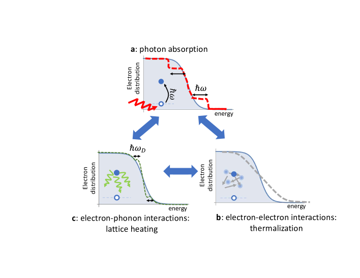
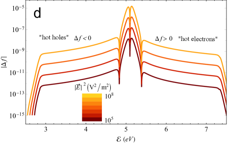
Figure 1: Full non-equilibrium electron distribution under illumination. The steady-state of the system is determined by the balance of three processes, shown on the background of the thermal distribution (Grey). a: absorption of photons by an electron, with an energy quanta $\hbar\omega$. b: electron (red) - phonon (green) scattering, which leads to lattice heating.c: electron-electron scattering, which leads to thermalization and electron heating. In addition, the excess thermal energy from the lattice can be transferred to the environment. d: Deviation from the equilibrium distribution at the ambient electron temperature, namely, $\Delta f\equiv f(\mathcal{E},T_{e},T_{ph})-f^{T}(\mathcal{E},T_{env})$, as a function of electron energy for various incoming field levels; the system is a bulk Ag illuminated by $\hbar\omega=2.25$eV photons, see all parameters values in Table A.2. Non-thermal hole densities, which correspond to $\Delta f<0$, are shown for simplicity in opposite sign. The dashed vertical line represents the Fermi energy. The various dips are artifacts of the semilogarithmic scale - they represent sign changes of $\Delta f$.

For energies beyond $\hbar\omega$ from the Fermi energy, the non-thermal distribution is much lower, as it requires multiple photon absorption . This implies that in order to efficiently harvest the excess energy of the non-thermal electrons, one has to limit the harvested energy to processes that require an energy smaller than $\hbar\omega$.

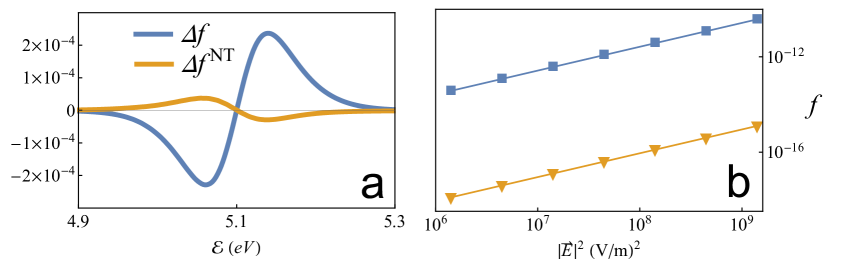
Figure 2: Non-thermal contribution to non-equilibrium. a: Comparison of the true non-equilibrium distribution $\Delta f^{NT}\equiv f(\mathcal{E},T_{e},T_{ph})-f^{T}(\mathcal{E},T_{e})$ with $\Delta f$ within the energy range close to the Fermi energy for $|\vec{E}|^{2}=10^{9}[V/m]$. The true non-equilibrium is smaller and of opposite sign, indicating on the presence of non-thermal holes (electrons) above (below) the Fermi energy. b: The populations $f(\mathcal{E})$ of electrons at $\mathcal{E}=1.8$ eV above the Fermi level (blue rectangles) and electrons at $\mathcal{E}=2.5$ eV ($>\hbar\omega$) above the Fermi level (yellow triangles), all as a function of local field, showing a quadratic dependence between illumination field and “hot” carrier population (with a similar slope).

The non-thermal electron distributions we obtained look similar to those obtained by calculations of the excitation rates due to photon absorption Atwater_Nat_Comm_2014 ; Manjavacas_Nordlander ; Munday_hot_es ; Louie_photocatalysis . However, as pointed out in Atwater_Nat_Comm_2014 ; Govorov_ACS_phot_2017 , this approach yields the correct electron distribution only immediately after illumination by an ultrashort pulse (essentially before any scattering processes take place); this distribution would be qualitatively similar to the steady-state distribution only if all other terms in the BE were energy-independent, which is not the case (see SI Section A.1 and Fig. 5). More specifically, this approach does not predict correctly the electron distribution near the Fermi energy; this means that the total energy stored in the electron system is not correctly accounted for and that the contribution of inter-band transitions to the non-equilibrium cannot be correctly determined. The main reason for these inaccuracies is that these studies did not correctly account for the electron and phonon temperatures, hence, the energy flow from the thermal electrons to the lattice such that quantitative conclusions on the distribution drawn in these studies should be taken with a grain of salt. Similar inaccuracies are found also in Govorov_1 ; Govorov_2 ; Govorov_ACS_phot_2017 ; Govorov_nature_nano .

On the other hand, these approaches can be used to provide a quantitative prediction of the electron distribution away from the Fermi energy, where $e-ph$ interactions are negligible (see (Dubi-Sivan-Faraday, , Section IIB)); peculiarly, however, this was not attempted previously Atwater_Nat_Comm_2014 ; Manjavacas_Nordlander ; Munday_hot_es ; Louie_photocatalysis , and instead, only claims about the qualitative features of the electron distributions were made.

Our calculations also show that the number of photo-generated high energy electrons $\Delta f^{NT}$ is independent of $G_{ph-env}$ (see Fig. 9 and discussion in SI Section A.2). Since $G_{ph-env}$ is proportional to the thermal conductivity of the host and inversely proportional to the particle surface area, this implies that if a specific application relies on the number of high energy electrons, then, it will be relatively insensitive to the thermal properties of the host and the particle size. Conversely, since the temperature rise is inversely proportional to $G_{ph-env}$ (see thermo-plasmonics-basics and Fig. 9), the difference in the photo-catalytic rate between the TiO₂ and SiO₂ substrates (compare Halas_dissociation_H2_TiO2 and Halas_H2_dissociation_SiO2 ) is likely a result of a mere temperature rise, but is not likely to be related to the number of photo-generated high energy electrons (see further discussion in Y2-eppur-si-riscalda ).

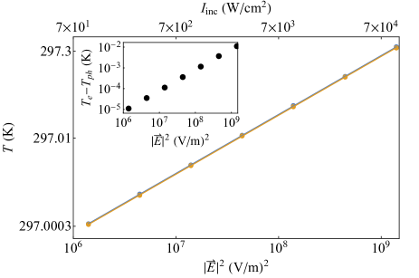
Figure 3: Temperature rise under illumination. The electron (blue) and lattice (orange) temperatures extracted from the data of Figs. 1-2 as a function of the local field (loglog scale), showing a linear dependence on field-squared (top $x$-axis show the corresponding incident intensity). Inset: difference between electron and phonon temperatures as a function of field squared, showing that (i) the difference is also linear, and (ii) several orders of magnitude smaller than the temperatures themselves (making the electron and phonon temperatures essentially equal).

Electron and phonon temperatures.  As pointed above, our approach allows a quantitative estimate of both electron and phonon temperatures. In Fig. 3, these are plotted (on a log-log scale) as a function of the local field squared $|\vec{E}|^{2}$ (also translated into incident illumination intensity $I_{inc}$ in the upper x-axis for the specific case of a 5nm Ag sphere). As seen, both temperatures grow linearly with $|\vec{E}|^{2}$ over many decades of the field, as in the classical (single temperature) approach thermo-plasmonics-review ; Abajo_nano-oven . In the inset we plot the difference between the electron and phonon temperatures as a function $|\vec{E}|^{2}$. This difference is also linear, and is seen to be much smaller (around two orders of magnitude) than the temperatures themselves. This is a nontrivial result, since the our non-equilibrium model equations exhibit an implicit nonlinear dependence on the temperatures. Fig. 3 also shows that $T_{e}$ is only slightly higher than $T_{ph}$. This provides the first (qualitative and quantitative) justification, to the best of our knowledge, for the use of the single temperature heat equation in the context of metallic nanostructures under illumination thermo-plasmonics-review ; Abajo_nano-oven ; more generally, it provides a detailed understanding of the origin of the single-temperature model, as well as the limits to its validity (as at high intensities the electron-phonon temperature difference may become substantial).

Efficiency.  Our approach allows us to deduce how the power density pumped into the metal by the absorbed photons splits into the non-thermal electrons and into heating the electrons and the phonons (see Fig. 4), providing a way to evaluate the efficiency of the non-thermal electron generation (detailed calculation described in SI Section A.1.7). Remarkably, one can see that the overall efficiency of the non-thermal electron generation is truly abysmal: At low intensities, the power channeled to the deviation from equilibrium ($W_{ex}^{NT}\equiv\int\mathcal{E}\rho_{e}(\mathcal{E})\left(\frac{\partial f^{NT}}{\partial t}\right)_{ex}d\mathcal{E}$) is more than 8(!) orders of magnitude lower than the power invested in the heating of the electrons and phonons (which are accordingly nearly similar). This is in correlation with the results of Fig. 1: most absorbed power leads to a change of the electron distribution near the Fermi energy, rather than to the generation of high energy electrons, as one might desire. This shows that any interpretation of experimental results which ignores electron and phonon heating should be taken with a grain of salt. It is thus the main result of the current study.

The performance of a “hot” electron system (say for catalysis or photo-detection, when electrons need to tunnel out of the nanoparticle) is essentially proportional to the electron distribution at the relevant energies (see SI Section A.1.8). A comparison with the pure thermal distribution of high energy electrons (Fig. 2) shows that the absolute electron population can be many orders of magnitude higher compared to the thermal distribution at the steady-state temperature. Such an enhancement was indeed observed in “hot” electron based photodetection devices Valentine_hot_e_review ; Halas_hot_es_photodetection , but not in “hot” electron photocatalysis chem_rev_photochemistry_2006 ; hot_e_review_Purdue ; plasmonic_photocatalysis_Linic ; plasmonic_photocatalysis_Clavero ; plasmonic-chemistry-Baffou ; hot_es_review_2015_Moskovits ; Govorov_nature_nano ; Manjavacas_Nordlander .

One can identify several pathways towards significant improvements of the efficiency of photo-generation of non-thermal electrons. In particular, as can be seen from Fig. 4, as the local field is increased, the power fraction going to non-equilibrium increases to $10^{-5}$. This improvement motivates the study of the non-thermal electron distribution for higher intensities. Such study, however, will require extending the existing formulation by extracting self-consistently also the metal permittivity from the non-equilibrium electron distribution $f$ (like done above for the electron temperature). Other pathways for improved “hot” electron harvesting may rely on interband transitions due to photons with energies far above the interband threshold Louie_photocatalysis ; Alivisatos_Toste , or optimizing the nanostructure geometry to minimize heating and maximize the local fields Fabrizio_hot_es , e.g., using few nm particles (which support the same number of non-thermal carriers but lower heating levels).

Finally, the formulation we developed serves as an essential first step towards realistic calculations of the complete energy harvesting process, including especially the tunneling process, and the interaction with the environment, be it a solution, gas phase or a semiconductor. Our formulation enables a quantitative comparison with experimental studies of all the above processes and the related devices. Similarly, our formulation can be used to separate thermal and non-thermal effects in many other solid-state systems away from equilibrium, in particular, semiconductor-based photovoltaic and thermo-photovoltaic systems.

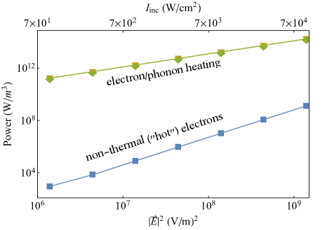
Figure 4: Power density and its distribution between the different channels. Power densities going into the thermal electron and lattice systems ($W_{e-e}$ in green diamonds and $W_{e-ph}$ in orange triangles, respectively), compared with the power going to the non-thermal electrons ($W_{ex}^{NT}$ in blue squares), all as a function of the local field. The power fraction that flows into the thermal channels (i.e., to heat the systems) is substantially larger than that going into generating non-thermal electrons.

Acknowledgements. The authors would like to thank G. Bartal, A. Govorov, J. Lischner, R. Oulton, A. Nitzan, S. Sarkar and I.W. Un for many fruitful discussions.

Appendix A Supplementary Information:
“Hot” electrons in metallic nanostructures - non-thermal carriers or heating?

A.1 Solution of the quantum-like Boltzmann equation

We determine the electron distribution in the conduction (sp) band, $f(\mathcal{E},T_{e},T_{ph})$, in a metal nanostructure under continuous wave (CW) illumination by solving the quantum-like Boltzmann equation (BE). This model is in wide use for such systems Ziman-book ; Ashcroft-Mermin ; Lundstrom-book ; non_eq_model_Lagendijk ; delFatti_nonequilib_2000 ; vallee_nonequilib_2003 ; Italians_hot_es ; Seidman-Nitzan-non-thermal-population-model ; It is valid for nanoparticles which are more than a few nm in size (hence, not requiring energy discretization) GdA_hot_es ; Govorov_ACS_phot_2017 and for systems where coherence and correlations between electrons are negligible. The latter assumption holds for a simple metal at room temperatures (or higher), as it has a large density of electrons and fast collision mechanisms. In order to include quantum finite size effects or quantum coherence effects, one can use the known relation between the discretized BE and quantum master equations Goodnick_DM_BE ; Chattah_DM_BE or by replacing the BE by that equation Govorov_1 ; Govorov_2 ; Govorov_ACS_phot_2017 .

For simplicity, we consider a quasi-free electron gas such that the conduction band is purely parabolic (with a Fermi energy of $\mathcal{E}_{F}=5.1$eV and total size of $\mathcal{E}_{max}=9$eV, typical to Ag, see Ashcroft-Mermin ). This allows us to represent the electron states in terms of energy $\mathcal{E}$ rather than momentum. We also neglect interband ($d$ to $sp$) transitions - these have a small role when describing metals like Al illuminated by visible light, Ag for wavelengths longer than about $500$nm or so, or Au for near infrared frequencies, where a dominantly Drude response is exhibited. Furthermore, as noted in Govorov_ACS_phot_2017 , interband transitions are not likely to generate electrons with energies far above the Fermi level unless the photon energy is much higher than the bandgap energy.

The resulting Boltzmann equation is

$$\frac{\partial f\left(\mathcal{E}(\vec{k});T_{e},T_{ph}\right)}{\partial t} = \underbrace{\left(\frac{\partial f}{\partial t}\right)_{ex}}_{photon\ absorption}+\underbrace{\left(\frac{\partial f}{\partial t}\right)_{e-ph}}_{e-ph\ collisions}+\underbrace{\left(\frac{\partial f}{\partial t}\right)_{e-e}}_{e-e\ collisions},$$ (4)

where $f$ is the electron distribution function at an energy $\mathcal{E}$, electron temperature $T_{e}$ and phonon temperature $T_{ph}$, representing the population probability of electrons in a system characterized by a continuum of states within the conduction band. The first term on the right-hand-side (RHS) of Eq. (4) describes excitation of conduction electrons due to photon absorption, see SI Section A.1.1 below for its explicit form. The second term on the RHS of Eq. (4) describes energy relaxation due to collisions between electrons and phonons, see SI Section A.1.2 below for its explicit form. This interaction makes the electrons in our model only quasi-free. The third term on the RHS of Eq. (4) (see SI Section A.1.3 below for its explicit form) represents the thermalization induced by $e-e$ collisions, i.e., the convergence of the non-thermal population into the thermalized Fermi-Dirac distribution, given by

$$f^{T}\left(\mathcal{E};T_{e}\right)=\left(1+e^{(\mathcal{E}-\mathcal{E}_{F})/k_{B}T_{e}}\right)^{-1},$$ (5)

where $k_{B}$ is the Boltzmann constant .

Note that our model does not require indicating what is the exact nature of the various collisions (Landau damping, surface/phonon-assisted, etc., see discussions in hot_es_Atwater ; Khurgin_Landau_damping ; GdA_hot_es ; Louie_photocatalysis ), but rather, it accounts only for their cumulative rate. Within this description, it was shown in hot_es_Atwater ; GdA_hot_es that the total electron collision time is independent of the size of the metal nanoparticle . Our model also does not account for electron acceleration due to the force exerted on them by the electric field (which involves a classical description, see SI Section A.1.1 below), nor for drift due to its gradients or due to temperature gradients; these effects will be small in the regime of intensities considered in our study, especially for few nm (spherical) particles (see also SI Section A.2 below) thermo-plasmonics-basics ; Un-Sivan-size-thermal-effect . Similar simplifications were adopted in most previous studies of this problem, e.g., Govorov_1 ; Govorov_2 ; Govorov_3 ; Manjavacas_Nordlander ; GdA_hot_es ; Govorov_ACS_phot_2017 ). These neglected effects can be implemented in our formalism in a straightforward way.

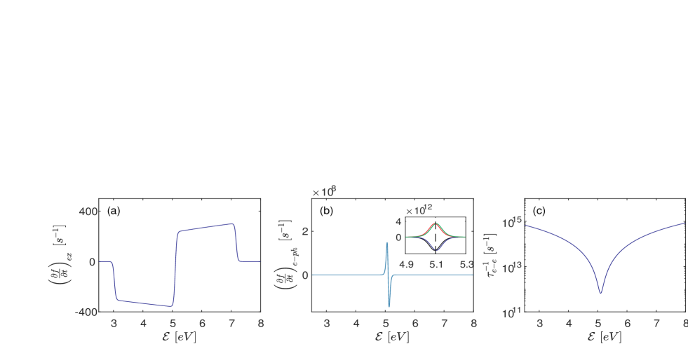
Figure 5: (Color online) (a) $\left(\frac{\partial f}{\partial t}\right)_{ex}$ (12) as a function of electron energy for a local field of $|\vec{E}|=7\cdot 10^{3}V/m$. (b) The $e-ph$ collision rate (13) as a function of electron energy for $T_{e}-T_{ph}=0.2^{\circ}$K. The inset shows the four competing phonon generation/absorption processes. (c) The $e-e$ collision rate as a function of electron energy, as given by Fermi liquid theory, Eq. (14).

Finally, we emphasize that the results shown in the main text are not sensitive to the details of the general model. In fact, our procedure can be made more system specific; for instance, the metal band structure can be taken into account hot_es_Atwater ; Louie_photocatalysis , few nm nanoparticles can be studied by writing the BE in momentum space and discretizing it GdA_hot_es , and further quantum effects may be considered by replacing the BE by a quantum master equation Govorov_1 ; Govorov_2 ; Govorov_ACS_phot_2017 . We do not expect any such change to have more than a moderate quantitative effect on the results shown below.

The steady-state solution of Eqs. (1)-(3) was attained numerically by writing the (thermal) electron and phonon energies as the product of the corresponding heat capacities and temperatures (see SI Section A.1.7) and letting the system evolve naturally to the steady-state by ramping up slowly the electric field. Table 1 shows the values of all parameters used in our simulations. We observe that the results are insensitive to the initial conditions and choice of various parameter values.

Table 1: Parameters used in the simulations; values chosen for (low quality Indian_Ag_ellipsometry_2014 ) $5$nm Ag sphere.

parameter	parameter symbol	value
photon wavelength	$\lambda$	$2.25$eV
metal permittivity	$\epsilon_{Ag}(\lambda)$	$-8.5+1.8i$ Indian_Ag_ellipsometry_2014
host permittivity	$\epsilon_{h}$	$4.25$
Fermi energy	$\mathcal{E}_{F}$	$5.1$eV
conduction band width	$\mathcal{E}_{max}$	$9$eV
chemical potential	$\mu$	$5.1$eV
ph-env coupling	$G_{ph-env}$	$5\cdot 10^{14}W/m^{3}K$
electron density	$n_{e}$	$5.86\cdot 10^{28}m^{-3}$
speed of sound	$v_{ph}$	$3650$ m/s
environment temperature	$T_{env}$	$297K$
electron mass	$m_{e}$	$9.1\cdot 10^{31}$ kg

A.1.1 The quantum mechanical excitation term

Usually, the BE is regarded as a (semi-)classical model of electron dynamics. Indeed, several popular textbooks draw the links between the BE to the classical model of an electron motion in an electric field (e.g., Ziman-book ; Ashcroft-Mermin ; Dressel-Gruner-book ; Marini_faraday_discuss_2019 ). In this case, the change of momentum of the electrons (acceleration) due to the force exerted on them by the electric field corresponds to a coherent excitation term, i.e., a term which is proportional to $\frac{\partial}{\partial\mathcal{E}}\frac{\partial\mathcal{E}}{\partial\vec{k}}\cdot\frac{\partial\vec{k}}{\partial t}\sim\vec{v}\cdot\vec{E}$. However, since it relies on a classical field, this expression describes the photon-electron interaction correctly only if the energy imparted on the electron by the electric field is much greater than the energy of a single photon non_eq_model_Rethfeld . Since this is not the case, this term does not allow one to derive correctly the non-equilibrium distribution; in fact, this failure to produce experimental observations triggered Einstein to employ a quantized model for the photo-electric effect, and eventually led to the creation of quantum mechanics theory, as we know it.

In order to circumvent this problem within the BE, frequently the (semi-)classical (linear ($\sim\vec{E}$), coherent) excitation term is replaced by a quantum-like ($\sim|\vec{E}|^{2}$, incoherent) term derived from the Fermi golden rule delFatti_nonequilib_2000 ; vallee_nonequilib_2003 ; Italians_hot_es ; GdA_hot_es ; Manjavacas_Nordlander ; Seidman-Nitzan-non-thermal-population-model . Early derivations of this term (e.g. delFatti_nonequilib_2000 ) did not supply a rigorous expression for its magnitude, but rather fit its magnitude to experimental results. Later studies attempted to link the magnitude of this term to the total absorbed power Italians_hot_es . A systematic derivation was provided in GdA_hot_es .

Here, we employ the simpler, elegant expression proposed in Seidman-Nitzan-non-thermal-population-model , namely, we define $A(\mathcal{E};\omega)$ such that $A(\mathcal{E};\omega)d\omega d\mathcal{E}$ is the (joint) probability of photon absorption of frequency between $\omega$ and $\omega+d\omega$ for final energy $\mathcal{E}$ measured with respect to the bottom of the band at $\mathcal{E}=0$. We define this probability as

$$A(\mathcal{E}_{final}=\mathcal{E};\omega)=\frac{n_{A}(\omega)}{N_{A}}\frac{D_{J}(\mathcal{E},\mathcal{E}-\hbar\omega)\rho_{J}(\mathcal{E},\mathcal{E}-\hbar\omega)}{\int D_{J}(\mathcal{E},\mathcal{E}-\hbar\omega)\rho_{J}(\mathcal{E},\mathcal{E}-\hbar\omega)d\mathcal{E}},$$ (6)

where $D_{J}(\mathcal{E}_{final},\mathcal{E}_{initial})$ is the squared magnitude of a transition matrix element for the electronic process $\mathcal{E}_{initial}\to\mathcal{E}_{final}$; Further, $\rho_{J}$ is the population-weighted density of pair states,

$$\rho_{J}(\mathcal{E}_{final},\mathcal{E}_{initial})=\left[f(\mathcal{E}_{initial})\rho_{e}(\mathcal{E}_{initial})\right]\left[(1-f(\mathcal{E}_{final})\rho_{e}(\mathcal{E}_{final})\right],$$ (7)

and $\rho_{e}=\frac{3n_{e}}{2\mathcal{E}_{F}}\sqrt{\frac{\mathcal{E}}{\mathcal{E}_{F}}}$ is the density of states of a free electron gas Ashcroft-Mermin , $n_{e}$ being the electron density. Finally, $n_{A}(\omega)$ is the number density of absorbed $\hbar\omega$ photons per unit time between $\omega$ and $\omega+d\omega$ and $N_{A}=\int d\omega n_{A}(\omega)$ is the total number density of absorbed photons per unit time. For CW illumination, it is given by

$$N_{A}=\frac{\langle p_{abs}\left(\vec{r},t\right)\rangle_{t}}{\hbar\omega},$$ (8)

where the absorbed optical power density (in units of $W/m^{3}$) is given by the Poynting vector Jackson-book , namely,

$$\langle p_{abs}\left(t\right)\rangle_{t}=\omega\epsilon^{\prime\prime}(\omega,T_{e},T_{ph})\langle\vec{E}(t)\cdot\vec{E}(t)\rangle_{t},$$ (9)

where the temporal averaging, $\langle\rangle_{t}$, is performed over a single optical cycle such that only the time-independent component remains. Note that the absorption lineshape arises naturally from the spectral dependence of the local electric field in Eq. (9); it depends on the nanostructure geometry and the permittivities of its constituents. This way, there is no need to introduce the lineshape phenomenologically as done in Seidman-Nitzan-non-thermal-population-model .

The absorption probability of a $\hbar\omega$ photon, $A$ (6), satisfies

$$\int_{0}^{\infty}A(\mathcal{E};\omega)d\mathcal{E}=\frac{n_{A}(\omega)}{N_{A}},$$ (10)

and the net change of electronic population at energy $\mathcal{E}$ per unit time and energy at time $t$ due to absorption is $N_{A}\phi_{A}$, where

$$\phi_{A}(\mathcal{E};\omega)=\int_{0}^{\infty}d\omega[A(\mathcal{E};\omega)-A(\mathcal{E}+\hbar\omega;\omega)],$$ (11)

is a quantity describing the total (probability of a) population change at energy $\mathcal{E}$ per unit time and energy at time $t$.

Altogether, the change of population due to photon excitation is given by

$$\left(\frac{\partial f}{\partial t}\right)_{ex}(\mathcal{E})=\frac{N_{A}\phi_{A}(\mathcal{E})}{\rho_{e}(\mathcal{E})},$$ (12)

so that electron number conservation is ensured, $\int d\mathcal{E}\rho_{e}(\mathcal{E})\left(\frac{\partial f}{\partial t}\right)_{ex}(\mathcal{E})\sim\int d\mathcal{E}\phi_{A}(\mathcal{E})=0$.

The functional form of Eq. (12) is shown in Fig. 5(a) - one can see a roughly flat, $\hbar\omega$-wide region of positive rate above the Fermi energy, and a corresponding negative regime below the Fermi energy. In that regard, the incoherent, quantum-like, $|\vec{E}|^{2}$ excitation term reproduces the predictions of the photoelectric effect. The slight asymmetry originates from the density of states $\rho_{e}(\mathcal{E})$ . Some earlier papers, e.g., Munday_hot_es (and potentially, also Manjavacas_Nordlander ) used excitation rates similar to those of Eq. (12) to qualitatively describe the steady-state “hot” electron density. However, such a qualitative estimate is appropriate only in case all other terms in the underlying equation are energy-independent. Clearly, from Fig. 5, this is not generically the case. As explained in more detail in Dubi-Sivan-Faraday , this approach does not describe correctly the electron distribution near the Fermi energy, but it can describe the electron distribution correctly far from the Fermi energy (via multiplication by the $e-e$ collision time). Unfortunately, the former effect is orders of magnitude more important.

Note that in our approach, we effectively assume that momentum is conserved for all transitions. A more accurate description requires one to distinguish between the electron states according to their momentum, as done e.g., in vallee_nonequilib_2003 for a continuum of electron states and in GdA_hot_es ; Govorov_ACS_phot_2017 for discretized electron states. However, it is worth noting in this context that the numerical results in Govorov_ACS_phot_2017 show that when considering an ensemble of many nanoparticles with a variation in shape (up to 40%), quantization effects nearly disappear even for a 2nm (spherical) particle. Indeed, the analytical result (red lines in Figs. 4 and 5 of Govorov_ACS_phot_2017 ) for the high-energy carrier generation rate, obtained by taking the continuum state limit, is very similar to the exact discrete calculation averaged over the particle sizes. This shows that neglecting the possibility of momentum mismatch (which is the effective meaning of avoiding the energy state quantization, as essentially done in our calculations) provides a rather tight upper limit estimate. Having said that, we bear in mind that quantization effects may still be relevant in highly regular nanoparticle distributions, ordered nanoparticle arrays or single nanoparticle experiments.

A.1.2 The $e-ph$ collision term

In delFatti_nonequilib_2000 , the rate of change of $f$ due to $e-ph$ collisions is derived from the Bloch-Boltzmann-Peierls form Ziman-book ; PB_Allen_e_ph_scattering ^,, giving

$$\!\!\!\!\!\!\!\!\left(\frac{\partial f}{\partial t}\right)_{e-ph} =-\frac{\mathcal{X}^{2}\sqrt{m_{eff}^{*}}}{4\pi\rho\sqrt{2\mathcal{E}}}\frac{1}{\hbar v_{ph}}\int_{0}^{\mathcal{E}_{D}}d\mathcal{E}_{ph}\mathcal{E}_{ph}^{2}\big{\{}f(\mathcal{E})\left([1-f(\mathcal{E}+\mathcal{E}_{ph})]n(\mathcal{E}_{ph})+[1-f(\mathcal{E}-\mathcal{E}_{ph})][n(\mathcal{E}_{ph})+1]\right)$$ (13)

$$-[1-f(\mathcal{E})]\left[f(\mathcal{E}+\mathcal{E}_{ph})[n(\mathcal{E}_{ph})+1]+f(\mathcal{E}-\mathcal{E}_{ph})n(\mathcal{E}_{ph})\right]\big{\}}.$$

Here, $\mathcal{X}\sim 2\mathcal{E}_{F}/3$ is the effective deformation potential delFatti_nonequilib_2000 , $\rho$ is the material density and $m_{eff}^{*}$ is the effective electron mass . For simplicity, we further assume that the phonon system is in equilibrium, so that $n(\mathcal{E}_{ph})=n^{T}(\mathcal{E}_{ph};T_{ph})=\left(e^{\frac{\mathcal{E}_{ph}}{k_{B}T_{ph}}}-1\right)^{-1}$ is the Bose-Einstein distribution function where $\mathcal{E}_{ph}$ is the phonon energy and $T_{ph}$ is the phonon temperature. Eq. (13) relies on the Debye model , namely, a linear dispersion relation for the phonons is assumed, $\mathcal{E}_{ph}=v_{ph}\hbar|q|$, where $v_{ph}$ is the speed of sound ($\cong 3650$m/s in Ag) and $q$ is the phonon momentum. Beyond the Debye energy, $\mathcal{E}_{D}=k_{B}T_{D}\cong 0.015$eV for Ag, the density of phonon states vanishes. Previous work emphasized the insensitivity of the non-equilibrium dynamics to the phonon density of states and dispersion relations, thus, justifying the adoption of this simple model delFatti_nonequilib_2000 ; Brown_PRB_2016 and the neglect of the phonon non-equilibrium. More advanced models that account also for the possible non-equilibrium of the lattice exist (see e.g., in Italians_hot_es ; Baranov_Kabanov_2014 ) but are relatively rare.

The two terms associated with $f(\mathcal{E}+\mathcal{E}_{ph})$ describe phonon absorption, whereas the two terms associated with $f(\mathcal{E}-\mathcal{E}_{ph})$ describe phonon emission. Fig. 5(b) shows the energy dependence of these four different processes described by Eq. (13) for $T_{e}-T_{ph}=0.2^{\circ}$K, neglecting the small non-thermal part of the distribution (justified a-posteriory). For this temperature difference, an estimate based on the relaxation time approximation for $e-ph$ collisions allows us to relate the magnitude of each term ($\sim 10^{12}/sec$) to a collision rate of $\sim 10$fs, in accord with the value sometimes adopted within this context Dressel-Gruner-book . However, since these four processes compete with each other, the resulting total change of the distribution due to $e-ph$ collisions is several orders of magnitude slower. Overall, one can see that (13) has a rather symmetric, $\sim\hbar\omega_{D}$-wide Lorentz-like lineshape. For $T_{e}>T_{ph}$, the rate is negative (positive) above (below) the Fermi energy, reflecting the higher likelihood of phonon emission processes, i.e., that energy is transferred from the electrons to the phonons. In order to see this more clearly, we can calculate the rate of energy transfer between the electrons and phonons by multiplying by $\mathcal{E}\rho_{e}(\mathcal{E})$ and integrating over all electron energies. The resulting integral, defined as $W_{e-ph}\equiv-\int_{0}^{\infty}\mathcal{E}\rho_{e}(\mathcal{E})\left(\frac{\partial f}{\partial t}\right)_{e-ph}d\mathcal{E}$, is hardly distinguishable from its thermal counterpart, $W_{e-ph}^{T}\equiv-\int_{0}^{\infty}\mathcal{E}\rho_{e}(\mathcal{E})\left(\frac{\partial f^{T}}{\partial t}\right)_{e-ph}d\mathcal{E}$, which is usually represented by $G_{e-ph}\left(T_{e}-T_{ph}\right)$ PB_Allen_e_ph_scattering . For $T_{e}>T_{ph}$, the factor $\mathcal{E}\rho_{e}(\mathcal{E})$ weighs favourably the region above the Fermi energy, such that $W_{e-ph}$ and $W^{T}_{e-ph}$ are positive. In Brown_PRB_2016 , an ab-initio, parameter-free derivation of the electron-phonon coupling coefficient based on density functional theory found $G_{e-ph}\sim 3\cdot 10^{16}W/m^{3}K$ for Ag, in agreement with values found in previous works el_lat_relaxation ; PB_Allen_e_ph_scattering ; delFatti_nonequilib_2000 ; Italians_hot_es ; contribution_to_heat_cap_el_ph_inter ; G_nonthermal_Hopkins_2015 , and with a negligible temperature-dependence, up to about $3000^{\circ}$K.

We note that our approach accounts for the mutual effect $e-e$ collisions have on $e-ph$ collisions non_eq_model_Lagendijk , since $e-ph$ collisions are treated by the $f$-dependent rate (13) (rather than within the relaxation time approximation).

A.1.3 The $e-e$ collision term

A.1.4 The $e-e$ collision rate

The rate of $e-e$ collisions near thermal equilibrium is usually slower than the $e-ph$ collision rate (order of picoseconds) since they involve only deviations from the independent electron approximation Ashcroft-Mermin . However, away from thermal equilibrium, the $e-e$ collision rates of high energy non-thermal electrons increase substantially and can become comparable to the $e-ph$ collision rate or even faster (see Fig. 5(c)). Specifically, by Landau’s Fermi liquid Theory (FLT) Quantum-Liquid-Coleman , the (effective) $e-e$ collision rate is given by

$$\tau_{e-e}^{-1}(\mathcal{E})=K\left[\left(\pi k_{B}T_{e}\right)^{2}+\left(\mathcal{E}-\mathcal{E}_{F}\right)^{2}\right],$$ (14)

where $K={m_{eff}^{*}}^{3}/8\pi^{4}\hbar^{6}W_{e-e}$ is the characteristic $e-e$ scattering constant that contains the angular-averaged scattering probability $W_{e-e}$ and the effective mass of the electron, $m_{eff}^{*}$; for Au and Ag, $K=2\cdot 10^{14}/eV^{2}\ s$ non_eq_model_Lagendijk . Similar variations of this expressions within a continuum of states description were used e.g., in delFatti_nonequilib_2000 ; vallee_nonequilib_2003 ; Italians_hot_es in the context of ultrafast illumination. The more recent calculations of the $e-e$ collision rate within a discretized electron energy description, e.g., in GdA_hot_es ; hot_es_Atwater retrieved this functional dependence. Experimental data obtained via two photon photo-emission measurements are found in excellent agreement with the Fermi liquid based expression (14), see discussion in Italians_hot_es .

A.1.5 Energy conserving relaxation time approximation

Since $e-e$ collisions are elastic (and within the approximation adopted here, also isotropic) Lundstrom-book , we can adopt the relaxation time approximation for sufficiently small deviation from equilibrium, and write

$$(\Delta_{\tau}f)_{e-e}=-\frac{f(\mathcal{E},T_{e},T_{ph})-f^{T}(\mathcal{E},T_{e})}{\tau_{e-e}(\mathcal{E})}.$$ (15)

However, we note that the regular $e-e$ term does not conserve the energy of the electron system as a whole (although it is supposed to, by the elastic nature of $e-e$ collisions). As a remedy, we introduce a term $\mathcal{F}_{e-e}(\mathcal{E})$, defined by the condition $\int_{0}^{\infty}\mathcal{E}\rho_{e}(\mathcal{E})\left[(\Delta_{\tau}f)_{e-e}+\mathcal{F}_{e-e}(\mathcal{E})\right]d\mathcal{E}=0$. This additional term ensures that the electron energy, defined as $\mathcal{U}_{e}\equiv\int_{0}^{\infty}\mathcal{E}\rho_{e}(\mathcal{E})f(\mathcal{E},T_{e},T_{ph})d\mathcal{E}$, is conserved. Such a term is regularly included in Boltzmann models of fluid dynamics, where it is known as the Lorentz term Hauge-Boltzmann-Lorentz , but to our knowledge, was not employed in the context of illuminated metal nanostructures . Thus, overall, we have

$$\left(\frac{\partial f}{\partial t}\right)_{e-e}=(\Delta_{\tau}f)_{e-e}+\mathcal{F}_{e-e}(\mathcal{E}).$$ (16)

The absence of this term in previous steady-state derivations of the electron distribution (e.g., in Govorov_1 ; Govorov_2 ; Govorov_ACS_phot_2017 ) mean that energy is not conserved in these studies; Nevertheless, this specific effect is relatively small.

A.1.6 Comparison between different scattering time functions

The results in the main text were obtained using an $e-e$ collision time of the form (14). The coefficient $K$ was found using a fit to the calculations of Ref. GdA_hot_es . In addition, we performed the same calculation with a phenomenological scattering time of the form $\tau_{e-e}(\mathcal{E})=e^{(1/(a+b\mathcal{E}}$), with a = 0.08585, b = 0.1278 eV^-1 (which decays slightly faster than the usual energy-dependence of the FLT); this seems to fit the data of Ref. GdA_hot_es better. In Fig. 6 we show the original data of Ref. (GdA_hot_es, , Fig. 6) and the fits to the standard FLT form (14) and the phenomenological form.

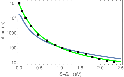
Figure 6: (Color online) The $e-e$ scattering time, evaluated by averaging over the data of from Ref. GdA_hot_es (black squares). Solid blue line is a fit to the standard (Fermi liquid) collision time (14), and the solid green line are fits to the phenomenological form defined in the text.

In Fig. 7 we show the “hot” electron distribution evaluated with these two forms for the $e-e$ collision time, the FLT one and the phenomenological one. As can be seen, while the distributions are slightly different, the difference is essentially quantitative. The electron and phonon temperatures were found to be identical for the 2 expressions for $\tau_{e-e}$ (within our numerical accuracy for the 2 cases).

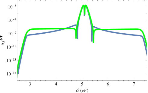
Figure 7: (Color online) Non-equilibrium electron distributions (see main text) for the two forms of $e-e$ scattering time, showing only a qualitative difference.

A.1.7 Evaluating the power density for different process

The formalism presented in this manuscript allows us to evaluate the power density that goes into heating the electrons and phonons, and the power that goes into generating non-thermal carriers.

To evaluate this, we start with the general expression for the total energy of the electron system, $\mathcal{U}_{e}$ defined above. Formally taking the time derivative gives the total power output of the electron system (which, at steady-state, vanishes by definition),

$$\frac{d\mathcal{U}_{e}}{dt}=\int\mathcal{E}\rho_{e}(\mathcal{E})\left(\frac{\partial f}{\partial t}\right)d\mathcal{E}.$$ (17)

From Eq. (1), one can formally break $\left(\frac{\partial f}{\partial t}\right)$ into different contributions. Plugging these contributions into Eq. (17) the power that goes into the difference energy channels. Specifically, substituting $\left(\frac{\partial f}{\partial t}\right)_{ex}$ gives the expression for the total power that is pumped into the electronic system by the photons.

Similarly, our formalism provides a natural way to distinguish between thermal and non-thermal contributions, since the steady-state distribution is naturally a-priori defined as $f(\mathcal{E})=f^{T}(\mathcal{E},T_{e})+f^{NT}(\mathcal{E})$. The first term is a thermal distribution with the (elevated) steady-state electron temperature, and the second term is the non-thermal distribution. Thus, substituting these into the expression for power gives the power $W^{T}$ that goes into the thermal part of the electron distribution (i.e., that goes into electron heating) and the power $W^{NT}$ that goes into generating non-thermal carriers, namely,

$$W^{T} = \int\mathcal{E}\rho_{e}(\mathcal{E})\left[\left(\frac{\partial f}{\partial t}\right)_{ex}\right]_{f=f^{T}}d\mathcal{E},$$ (18)

$$W^{NT} = \int\mathcal{E}\rho_{e}(\mathcal{E})\left[\left(\frac{\partial f}{\partial t}\right)_{ex}\right]_{f=f^{NT}}d\mathcal{E}.$$ (19)

A.1.8 Electron tunneling from the nanoparticle

The use of plasmonic naonparticles for applications requires that the “hot” electrons tunnel out of the nanoparticle in order to perform some function, be it tunneling into a molecular orbital for photocatalysis or across a Schottky barrier with a semiconductor for detection. The underlying assumption of much of the literature is that if such a process occurs at a given energy, then, the efficiency of the process will be proportional to the electron distribution at that energy. For example, in discussing tunneling across a barrier, then the eficiency of the process will be simply an integral over the electron distribution function over energies higher than the barrier energy (with some weight). Similarly, for tunneling into a molecular level, the efficiency will be proportional to the electron distribution at that energy.

In a recent paper Dubi-Sivan-Faraday we have shown that this is indeed the case for photo-catalysis, as long as the tunneling time is long compared to all other timescales, most importantly the $e-e$ scattering time. The argument relies on evaluating the distribution function in the presence of a tunneling term. We start by describing a tunneling term of the form $g(\varepsilon)f(\varepsilon)$, where $f$ is the distribution, and $g(\varepsilon)$ is some kernel, describing the tunneling rate per energy. Importantly, (i) $g$ is independent of the distribution and (ii) is localized at energies far from the Fermi energy, where the distribution is small (in fact, it could be a step-like function, for example if there is tunneling through a Schottky barrier, but here we have in mind photo-catalysis. The explanations below actually apply for both classes of applications).

Now, assuming that we know the steady-state distribution $f_{0}(\varepsilon)$, we look for a correction to it, $f=f_{0}+f_{1}$. The next step is to linearize the bare Liouvillian (i.e. the right-hand-side of the Boltzmann equation without the tunnelling term). Then, for the steady-state we have

$$0=\alpha(\varepsilon)f_{1}(\varepsilon)+g(\varepsilon)(f_{0}(\varepsilon)+f_{1}(\varepsilon)),$$ (20)

where $\alpha(\varepsilon)$ is the linearization term. This equation can easily be solved to give $f_{1}=\frac{g}{g+\alpha}f_{0}$. Now, as long as the dependence of $\alpha$ on energy is rather weak (which is indeed the case for both $e-e$ collision time and the excitation term), and the dependence of $f_{0}$ itself on $\varepsilon$ is also weak, the correction to the distribution function is simply proportional to the tunneling term $g(\varepsilon)$.

In order to test this (rather simple) estimate, we ran our calculation with an additional tunneling term of the form $-\gamma_{T}g(\varepsilon)f(\varepsilon)$, where $\gamma_{T}=10^{13}$Hz and $10^{15}$Hz, corresponding to a slow ($100$ femtosecond) and fast (few femtosecond) tunneling time (which is extremely fast, as realistic tunneling times were shown to be as short as 100 fs only in the best case scenario, see e.g., Uriel_Schottky_2018 ); $g$ is centered at $\approx 1.5$eV above the Fermi energy and has an energy width of a few hundreds of meV. In Fig. 8 we show the electron distribution with the tunneling terms, and the approximation (20). As can be seen, for $\gamma_{T}=10^{13}$Hz the approximation above is excellent.

Even more surprising and interesting, while for $\gamma_{T}=10^{15}$Hz there should be a difference (because formally we are outside the regime of the approximation), still the approximation seems very good. The conclusion we draw from this calculation is that, in principle, and over a wide range of parameters (and physical processes), knowledge of the bare distribution function (i.e., evaluated without a tunneling terms) provides an excellent indication to the performance of the “hot”-electron system as a functional device.

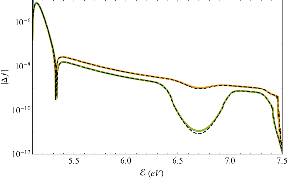
Figure 8: Non-equilibrium electron distribution with a tunneling term described in the text above, for $\gamma_{T}=10^{13}$Hz (orange line) and $10^{15}$Hz (green line). The dashed lines are the approximations (20).

A.2 Practical considerations

In order to avoid limiting the generality of our results, we did not indicate throughout the manuscript details of a specific nanostructure. In this SI Section, we discuss what needs to be done in order to apply our theory to a specific experimental configuration. For simplicity, we discuss nanospheres; extension of the discussion to other particle shapes is possible.

A.2.1 Local field

Throughout the manuscript, we treated $|\vec{E}|$ as a parameter representing the local field . In order to evaluate the non-thermal carrier density for an actual nanostructure configuration and illumination pattern, one needs to solve the Maxwell equations for the given configuration (for example, $\vec{E}=\left[3\epsilon_{h}/(2\epsilon_{h}+\epsilon_{m})\right]\vec{E}_{inc}$ for a small sphere illuminated uniformly) and apply our formulation locally, i.e., for each point in the nanostructure independently; this procedure was adopted in Govorov_ACS_phot_2017 and was complemented by surface/volume averaging. In that respect, the role of surface plasmon resonances in promoting “hot” carrier generation is obvious - at resonance, the local electric fields are enhanced, hence, the electron system is driven more strongly away from equilibrium.

For weak electric fields, like used in the current work and essentially in all relevant experiments (see e.g., Halas_dissociation_H2_TiO2 ; Halas_H2_dissociation_SiO2 , the distribution and temperatures can then be readily determined. For small spherical metal nanoparticles, the temperature(s) are uniform thermo-plasmonics-basics ; Un-Sivan-size-thermal-effect . The majority of previous theoretical studies relied on these same assumptions (e.g., Govorov_1 ; Manjavacas_Nordlander ; GdA_hot_es ).

For more complicated geometries, or for bigger nanostructures, the field may not be uniform. Nevertheless, the gradients of the electric fields are usually assumed to have a small effect on the electron distribution. The non-uniformity of the temperature is negligible, due to the relatively high thermal conductivity of the metal thermo-plasmonics-basics ; Un-Sivan-size-thermal-effect . Due to these reasons, these gradients were neglected in all previous studies; we adopt the same approach here. For higher fields, the optical and thermal properties of the metal may change due to the rise in temperature, requiring a fully self-consistent solution of the coupled Maxwell, Boltzmann and heat equations. Such a treatment is left to a future study.

A.2.2 Particle size

The size of the particle affects the field relatively weakly for sufficiently small size (for which the quasi-static approximation holds). However, as well-known thermo-plasmonics-basics , the nanoparticle temperature depends strongly on the particle size; for example, for nano-spheres, it grows quadratically with the radius $a$. In our formulation, this effect is accounted for via the value of the phonon-environment coupling, $G_{ph-env}$, which is usually calculated from first principles via molecular dynamics simulations, see e.g., Kapitza-Au-silicon ; Cahill-Kapitza-2006 ; Kapitza-NPs ; Munjiza_2014 . Overall, it scales inversely with the surface area vallee_nonequilib_2003 for nano-spheres; this is equivalent to assuming the total heat conductance to the environment is proportional to the particle surface area; this scaling facilitates estimates for non-spherical particles.

As pointed out in the main text, we have carried out additional calculations to demonstrate the dependence of electron distribution and temperatures on the particle size via $G_{ph-env}$. The original results (appearing in the main text figures; $5$nm particle size; $G_{ph-env}=5\times 10^{14}$ W/m³K Kippelen_JAP_2010 ) can now be compared to results for a particle which is 10 times bigger ($50$nm; $G_{ph-env}=5\times 10^{12}$ W/m³K). In Fig. 9(a), we plot the electron and phonon temperatures as a function of intensity for these two cases. As can be observed, the electron temperature rise is $\sim 100$-fold larger for the larger particle (compare to Fig. 3), namely, about 30K. However, the difference between the electron and phonon temperatures is roughly the same; indeed, it can be shown analytically to be proportional to the incoming intensity which is the same for both sets of simulations.

In Fig. 9(b) we plot the electron non-equilibrium distribution (specifically, the absolute value of the deviation of the electron distribution from the Fermi distribution, $|\Delta f|$) for the two particle sizes and for two illumination levels, $|\vec{E}|^{2}=1.4\times 10^{6}$, $1.4\times 10^{9}$(V/m)². It is readily seen that the only deviations between the large and small particle cases are at the vicinity of the Fermi energy, but the non-thermal parts of the distributions (i.e., further away from $\mathcal{E}_{F}$, where $\Delta f^{NT}\sim\Delta f$) are insensitive to the particle size. In particular, we find that the efficiency of non-thermal high energy electron generation is independent of particle size, but the overall heating scales as $a^{2}$, in agreement with the single temperature (classical) heat equation. Such correspondence is absent in the simulations in Govorov_ACS_phot_2017  . This also means that smaller particles give rise to a higher relative efficiency of non-thermal carrier generation. This prediction should motivate a careful, single particle study that will enable one to verify this prediction vs. potentially contradicting claims based on measurements from macroscopic nanoparticle suspensions.

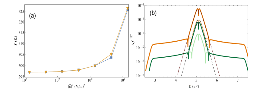
Figure 9: (a) Electron (yellow) and phonon (blue) temperatures as a function of $|\vec{E}|^{2}$, for a system with a host thermal conductivity $G_{ph-env}=5\times 10^{12}$ W/m³K, two orders of magnitude smaller than that employed in the simulations shown in Figs. 1-4 of the main text. Correspondingly, the temperature rise is much larger, as well as the difference between the electron and phonon temperatures. (b) Deviation of the non-equilibrium distribution from the thermal distribution for low host thermal conductivity and two intensities, $|\vec{E}|^{2}=1.4\times 10^{6},1.4\times 10^{8}$(V/m)² (dark green and dark orange lines, respectively). For comparison, the distributions from the high $G_{ph-env}$ values used in Fig. 1 are also plotted (light green and light orange solid lines). The dashed black lines show the differences between simple Fermi functions with $T=297.9$K (which is the electron temperature corresponding to the dark green line) and $T=325$K (which is the electron temperature corresponding to the dark orange line) to a Fermi function at ambient temperature of $297$K.

The results of Fig. 9(b) can be also interpreted in terms of the dependence of the non-thermal distribution on the host thermal conductivity. Indeed, the rate of energy density transfer to the environment $G_{ph-env}$ is also proportional to the thermal conductivity of the host vallee_nonequilib_2003 . Thus, the different curves in Fig. 9(a) can be also associated with a system with a host thermal conductivity which is two orders of magnitude lower than the one presented in the main text. As for the larger nanoparticle, the electron temperature rise and the difference between the electron and phonon temperatures, are higher, as expected - indeed, the heat flows away from the nanoparticle much more slowly for the larger nanoparticle. This shows, as stated in the main text, that if “hot” electrons play a dominant role in some experiment (e.g. in photo-catalysis), then, the experimental results should be unaffected by a change of host. Conversely, if the results are affected by a change of host material (as observed e.g., in Halas_dissociation_H2_TiO2 ; Halas_H2_dissociation_SiO2 ), then it is not likely that the reason for that is the number of “hot” electrons, but rather due to a thermal effect, or an altogether different chemical effect; for a detailed discussion, see also Y2-eppur-si-riscalda .

A.2.3 Surface scattering and quantum size effects

If one is interested in even smaller nanoparticles, then, within the energy state continuum description used in the current work, it may be necessary to account also for $e-surface$ collisions (the so-called “quantum size effects”), as noted as early as in Kreibig-book . As this effect does not involve conservation of electron momentum, it can be accounted for in our formulation by adding a relaxation time like term, $(f-f^{T})/\tau$, where $\tau$ is the time scale for these collisions which can be as fast as a few hundreds of femtoseconds in the case of a metal surface with atomic roughness Uriel_Schottky_2018 ; accordingly, it is practically negligible with respect to the $e-e$ and $e-ph$ collision rates. Depending on the nature of the $e-surface$ collisions, one may want to include/exclude them from the conservative term, $\mathcal{F}_{e-e}(\mathcal{E})$.

However, it should be noted that in more advanced models where the energy states are discretized (such that $e-surface$ collisions are accounted for inherently), e.g., GdA_hot_es ; Govorov_ACS_phot_2017 , the electronic states and the phononic states are extended throughout the bulk, and no “surface states” appear. One thus expects that in such calculations there will be no separate contribution from $e-surface$ collisions. In fact, in GdA_hot_es ; hot_es_Atwater it was shown that the electron collision time is independent of the nanoparticle size. All these results indicate that unlike previous claims hot_es_review_2015 “quantum size effects” have at most a small quantitative effect on the non-thermal carrier generation efficiency. This result was corroborated in Govorov_ACS_phot_2017 , see discussion at the end of Section A.1.1.

References

- (1) J. A. Schuller, E. S. Barnard, W. Cai, Y. C. Jun, J. S. White, and M. L. Brongersma. Plasmonics for extreme light concentration and manipulation. Nat. Mater., 9:193, 2010.
- (2) Editorial. Surface plasmon resurrection. Nat. Photon., 6:707, 2012.
- (3) I. Goykhman, B. Desiatov, J. Khurgin, J. Shappir, and U. Levy. Locally oxidized silicon surface-plasmon Schottky detector for telecom regime. Nano Lett., 11:2219–2224, 2011.
- (4) I. Goykhman, B. Desiatov, J. Khurgin, J. Shappir, and U. Levy. Waveguide based compact silicon Schottky photodetector with enhanced responsivity in the telecom spectral band. Opt. Exp., 20:28594, 2012.
- (5) W. Li and J. Valentine. Harvesting the loss: Surface plasmon-based hot electron photodetection. Nanophotonics, 6:177–191, 2016.
- (6) G. V. Naik and J. A. Dionne. Photon upconversion with hot carriers in plasmonic systems. Appl. Phys. Lett., 107:133902, 2015.
- (7) G. V. Naik, A. J. Welch, J. A. Briggs, M. L. Solomon, and J. A. Dionne. Hot-carrier-mediated photon upconversion in metal-decorated quantum wells. Nano Lett., 17:4583–4587, 2017.
- (8) K. Watanabe, D. Menzel, N. Nilius, and H.-J. Freund. Photochemistry on metal nanoparticles. Chem. Rev., 106:4301–4320, 2006.
- (9) A. Naldoni, F. Riboni, U. Guler, A. Boltasseva, V. M. Shalaev, and A. V. Kildishev. Solar-powered plasmon-enhanced heterogeneous catalysis. Nanophotonics, 5:112–133, 2016.
- (10) S. Linic, P. Christopher, and D.B. Ingram. Plasmonic-metal nanostructures for efficient conversion of solar to chemical energy. Nat. Materials, 10:911–921, 2011.
- (11) C. Clavero. Plasmon-induced hot-electron generation at nanoparticle/metal-oxide interfaces for photovoltaic and photocatalytic devices. Nat. Photon., 8:95–103, 2014.
- (12) G. Baffou and R. Quidant. Nanoplasmonics for chemistry. Chem. Soc. Rev., 43:3898, 2014.
- (13) M. Moskovits. The case for plasmon-derived hot carrier devices. Nature Nanotech., 10:6, 2015.
- (14) Kenneth O. Aruda, Mario Tagliazucchi, Christina M. Sweeney, Daniel C. Hannah, George C. Schatz, and Emily A. Weiss. Identification of parameters through which surface chemistry determines the lifetimes of hot electrons in small au nanoparticles. Proceedings of the National Academy of Sciences, 110(11):4212–4217, 2013.
- (15) S. Mubeen, J. Lee, N. Singh, S. Kraemer, G. D. Stucky, and M. Moskovits. An autonomous photosynthetic device in which all charge carriers derive from surface plasmons. Nat. Nanotech., 8:247–251, 2013.
- (16) K. Ueno, T. Oshikiri, X. Shi, Y. Zhong, and H. Misawa. Plasmon-induced artificial photosynthesis. Interface Focus, 5:20140082, 2014.
- (17) R. H. M. Groeneveld, R. Sprik, and A. Lagendijk. Femtosecond spectroscopy of electron-electron and electron-phonon energy relaxation in Ag and Au. Phys. Rev. B, 51:11433–11445, 1995.
- (18) N. Del Fatti, C. Voisin, M. Achermann, S. Tzortzakis, D. Christofilos, and F. Valleé. Nonequilibrium electron dynamics in noble metals. Phys. Rev. B, 61:16956–16966, 2000.
- (19) P. Grua, J. P. Morreeuw, H. Bercegol, G. Jonusauskas, and F. Valleé. Electron kinetics and emission for metal nanoparticles exposed to intense laser pulses. Phys. Rev. B, 68:035424, 2003.
- (20) L. D. Pietanza, G. Colonna, S. Longo, and M. Capitelli. Non-equilibrium electron and phonon dynamics in metals under femtosecond laser pulses. Eur. Phys. J. D, 45:369–389, 2007.
- (21) H. Harutyunyan, A. B. F. Martinson, D. Rosenmann, L. K. Khorashad, L. V. Besteiro, A. O. Govorov, and G. P. Wiederrecht. Anomalous ultrafast dynamics of hot plasmonic electrons in nanostructures with hot spots. Nature Nanotech., 10:770, 2015.
- (22) J. R. M. Saavedra, A. Asenjo-Garcia, and F. Javier Garcia de Abajo. Hot-electron dynamics and thermalization in small metallic nanoparticles. ACS Photonics, 3:1637–1646, 2016.
- (23) R. Sundararaman, P. Narang, A. S. Jermyn, W. A. Goddard, and H. A. Atwater. Theoretical predictions for hot-carrier generation from surface plasmon decay. Nature Communications, 5:5788, 2014.
- (24) M. Bernardi, J. Mustafa, J. B. Neaton, and S. G. Louie. Theory and computation of hot carriers generated by surface plasmon polaritons in noble metals. Nature Commun., 6:7044, 2015.
- (25) A. M. Brown, R. Sundararaman, P. Narang, A. M. Schwartzberg, W. A. Goddard, and H. A. Atwater. Experimental and ab initio ultrafast carrier dynamics in plasmonic nanoparticles. Phys. Rev. Lett., 118:087401, 2017.
- (26) A. O. Govorov, H. Zhang, and Y. K. Gun’ko. Theory of photoinjection of hot plasmonic carriers from metal nanostructures into semiconductors and surface molecules. J. Phys. Chem. C, 117:16616–16631, 2013.
- (27) H. Zhang and A. O. Govorov. Optical generation of hot plasmonic carriers in metal nanocrystals: The effects of shape and field enhancement. J. Phys. Chem. C, 118:7606–7614, 2014.
- (28) L. V. Besteiro, X.-T. Kong, Z. Wang, G. Hartland, and A. O. Govorov. Understanding hot-electron generation and plasmon relaxation in metal nanocrystals: Quantum and classical mechanisms. ACS Photonics, 4:2759–2781, 2017.
- (29) A. Puglisi, A. Sarracino, and A. Vulpiani. Temperature in and out of equilibrium: a review of concepts, tools and attempts. Physics Reports, 709–710:1–60, 2017.
- (30) Guillaume Baffou and Romain Quidant. Thermo-plasmonics: using metallic nanostructures as nano-sources of heat. Laser & Photonics Reviews, 7(2):171–187, 2013.
- (31) S. I. Anisimov, B. L. Kapeilovich, and T. I. Perelman. Electron emission from metal surfaces exposed to ultrashort laser pulses. Sov. Phys. JETP, 39:375–378, 1974.
- (32) L. Meng, R. Yu, M. Qiu, and F. J. García de Abajo. Plasmonic nano-oven by concatenation of multishell photothermal enhancement. ACS Nano, 11:7915–7924, 2019.
- (33) J. M. Ziman. Principles of the theory of solids. Cambridge University Press, 1972.
- (34) N. W. Ashcroft and N. D. Mermin. Solid state physics. Brooks/Cole, 1976.
- (35) D. Pines and P. Nozieres. The theory of quantum liquids. Benjamin, New York, New York, 1966.
- (36) M. Dressel and G. Grüner. Electrodynamics of solids - optical properties of electrons in matter. Cambridge University Press, 2002.
- (37) B. Rethfeld, A. Kaiser, M. Vicanek, and G. Simon. Ultrafast dynamics of nonequilibrium electrons in metals under femtosecond laser irradiation. Phys. Rev. B, 65:214303, 2002.
- (38) M. Kornbluth, A. Nitzan, and T. Seidman. Light-induced electronic non-equilibrium in plasmonic particles. J. Chem. Phys., 138:174707, 2013.
- (39) G. Baffou and R. Quidant. Thermo-plasmonics: using metallic nanostructures as nano-sources of heat. Laser Photon. Rev., 7:171–187, 2013.
- (40) A. Manjavacas, J. G. Liu, V. Kulkarni, and P. Nordlander. Plasmon-induced hot carriers in metallic nanoparticles. ACS Nano, 8:7630–7638, 2014.
- (41) P. B. Allen. Theory of thermal relaxation of electrons in metals. Phys. Rev. Lett., 59:1460–1463, 1987.
- (42) A. M. Brown, R. Sundararaman, P. Narang, W. A. Goddard, and H. A. Atwater. Nonradiative plasmon decay and hot carrier dynamics: Effects of phonons, surfaces, and geometry. ACS Nano, 10:957–966, 2016.
- (43) M. Lundstrom. Fundamentals of carrier transport. Addison-Wesley, 1990.
- (44) Y. Sivan, I. W. Un, and Y. Dubi. Assistance of plasmonic nanostructures to photocatalysis - just a regular heat source. Faraday Discussions, accepted, 2018.
- (45) S. Mukherjee, F. Libisch, N. Large, O. Neumann, L. V. Brown, J. Cheng, J. Britt Lassiter, E. A. Carter, P. Nordlander, and N. J. Halas. Hot electrons do the impossible: Plasmon-induced dissociation of H2 on Au. Nano Lett., 13:240–247, 2013.
- (46) T. Gong and J. N. Munday. Materials for hot carrier plasmonics. Optical Materials Express, 5:2501, 2015.
- (47) G. Baffou, R. Quidant, and F. J. Garcia de Abajo. Nanoscale control of optical heating in complex plasmonic systems. ACS Nano, 4:709–716, 2010.
- (48) S. Mukherjee, L. Zhou, A. Goodman, N. Large, C. Ayala-Orozco, Y. Zhang, P. Nordlander, and N. J. Halas. Hot-electron-induced dissociation of H2 on gold nanoparticles supported on SiO2. J. Am. Chem. Soc., 136:64–67, 2014.
- (49) Y. Sivan, I. W. Un, and Y. Dubi. Thermal effects - an alternative mechanism for plasmonic-assisted photo-catalysis. submitted; https://arxiv.org/abs/1902.03169, 2019.
- (50) A. Sobhani, M. W. Knight, Y. Wang, B. Y. Zheng, N. S. King, L. V. Brown, Z. Fang, P. Nordlander, and N. J. Halas. Narrowband photodetection in the near-infrared with a plasmon-induced hot electron device. Nat. Commun., 4:1643, 2013.
- (51) P. Christopher, H. Xin, A. Marimuthu, and S. Linic. Singular characteristics and unique chemical bond activation mechanisms of photocatalytic reactions on plasmonic nanostructures. Nat. Materials, 11:1044–1050, 2012.
- (52) J. Zhao, S. C. Nguyen, R. Ye, B. Ye, H. Weller, G. A. Somorjai, A. P. Alivisatos, and F. D. Toste. A comparison of photocatalytic activities of gold nanoparticles following plasmonic and interband excitation and a strategy for harnessing interband hot carriers for solution phase photocatalysis. ACS Cent. Sci., 3:482, 2017.
- (53) A. Giugni, B. Torre, A. Toma, M. Francardi, M. Malerba, A. Alabastri, R. Proietti Zaccaria, M. I. Stockman, and E. Di Fabrizio. Hot-electron nanoscopy using adiabatic compression of surface plasmons. Nat. Nanotech., 8:845–852, 2013.
- (54) D. Vasileska and S. M. Goodnick (eds.). Nano-electronic devices: Semiclassical and quantum transport modeling. Physics Reports, 478:71–120, 2009.
- (55) A. K. Chattah and M. O. Cáceres. Computing the quantum Boltzmann equation from a Kossakowski-Lindblad generator. In: O. Descalzi, J. Martínez, E. Tirapegui (eds.), Instabilities and Nonequilibrium Structures VII & VIII. Nonlinear Phenomena and Complex Systems. 8, 2004.
- (56) J. Khurgin, W.-Y. Tsai, D. P. Tsai, and G. Sun. Landau damping and limit to field confinement and enhancement in plasmonic dimers. ACS Photonics, 4:2871–2880, 2017.
- (57) I. W. Un and Y. Sivan. Size-dependence of the photothermal response of a single metal nanosphere. https://arxiv.org/abs/1907.01255, 2019.
- (58) A. Govorov and H. Zhang. Kinetic density functional theory for plasmonic nanostructures: Breaking of the plasmon peak in the quantum regime and generation of hot electrons. J. Phys. Chem. C, 119:6181–6194, 2015.
- (59) S. T. Sundari, S. Chandra, and A. K. Tyagi. Temperature dependent optical properties of silver from spectroscopic ellipsometry and density functional theory calculations. J. Appl. Phys., 033515:114, 2013.
- (60) A. Marini, A. Ciattoni, and C. Conti. Out-of-equilibrium electron dynamics of silver driven by ultrafast electromagnetic fields – a novel hydrodynamical approach. Faraday Discussions, 214:235, 2019.
- (61) J. D. Jackson. Classical electrodynamics. Wiley & Sons, 3rd edition, 1998.
- (62) A. M. Brown, R. Sundararaman, P. Narang, W. A. Goddard, and H. A. Atwater. Ab initio phonon coupling and optical response of hot electrons in plasmonic metals. Phys. Rev. B, 94:075120, 2016.
- (63) V. V. Baranov and V. V. Kabanov. Theory of the electron relaxation in metals excited by an ultrashort optical pump. Phys. Rev. B, 84:125102, 2014.
- (64) M.I. Kaganov, I.M. Lifshitz, and L.V. Tanatarov. Relaxation between electrons and crystalline lattices. Sov. Phys. JETP, 4:173–178, 1957.
- (65) P.E. Hopkins. Contributions of inter and intra-band excitations to electron heat capacity and electron-phonon coupling in noble metals. J. Heat Transfer, 132:014504, 2010.
- (66) A. Giri and P. E. Hopkins. Transient thermal and nonthermal electron and phonon relaxation after short-pulsed laser heating of metals. J. of Appl. Phys., 118:215101, 2015.
- (67) P. Coleman. Introduction to many body physics. Cambridge University Press, 2015.
- (68) E. H. Hauge. Exact and Chapman-Enskog solutions of the Boltzmann equation for the Lorentz model. The Physics of Fluids, 13:1201, 1970.
- (69) M. Grajower, J. Khurgin, and U. Levy. The role of surface roughness in plasmonic-assisted internal photoemission schottky photodetectors. ACS Photonics, 5:4030–4036, 2018.
- (70) J. C. Duda, C.-Y. P. Yang, B. M. Foley, R. Cheaito, D. L. Medlin, R. E. Jones, and P. E. Hopkins. Influence of interfacial properties on thermal transport at gold:silicon contacts. Appl. Phys. Lett., 102:081902, 2013.
- (71) H.-K. Lyeo and D. G. Cahill. Thermal conductance of interfaces between highly dissimilar materials. Phys. Rev. B, 73:144301, 2006.
- (72) S. Merabia, S. Shenogin, L. Joly, P. Keblinski, and J.-L. Barrata. Heat transfer from nanoparticles: A corresponding state analysis. Proc. Nat. Acad. Sci. U.S.A, 106:15113–15118, 2009.
- (73) X. Chen, A. Munjiza, K. Zhang, and D. Wen. Molecular dynamics simulation of heat transfer from a gold nanoparticle to a water pool. J. Phys. Chem. C, 118:1285 – 1293, 2014.
- (74) D. T. Owens, C. Fuentes-Hernandez, J. M. Hales, J. W. Perry, and B. Kippelen. A comprehensive analysis of the contributions to the nonlinear optical properties of thin Ag films. Journal of Applied Physics, 107:123114, 2010.
- (75) U. Kreibig and M. Vollmer. Optical Properties of Metal Clusters. Springer: Berlin, 1995.
- (76) M. L. Brongersma, N. J. Halas, and P. Nordlander. Plasmon-induced hot carrier science and technology. Nature Nanotech., 10:25, 2015.
- (77) A. O. Govorov and L. V. Besteiro. Comments on ””hot” electrons in metallic nanostructures – non-thermal carriers or heating?” and ”assistance of metal nanoparticles to photo-catalysis – nothing more than a classical heat source”. ArXiv, https://arxiv.org/abs/1906.06599, 2019.