On some curves with modified orthogonal frame in Euclidean 3-space

Abstract.

In this paper, we study helices and the Bertrand curves. We obtain some of the classification results of these curves with respect to the modified orthogonal frame in Euclidean 3-spaces.

1.
Introduction

In the classical study of differential geometry, curves satisfying particular relations with respect to their curvatures are of greater importance and applications. Helices and Bertrand curves are two among the prominent. A helix is a curve whose tangent makes a constant angle with a fixed direction(axis) [3, 8]. There is a famous classification of a general helix(Lancret theorem): a curve is a general helix iff $\frac{\kappa}{\tau}$= constant [21]. Izumiya and Takeuchi [9] defined a special class of helices called as slant helices, where the normal vector observes a constant angle with the fixed direction. They obtained a necessary and sufficient condition for a curve to be slant helix: a curve is a slant helix iff its geodesic curvature and the principal normal satisfying the expression

(1.1) $$\frac{\kappa^{2}}{(\kappa^{2}+\tau^{2})^{\frac{3}{2}}}\left(\frac{\tau}{\kappa}\right)^{\prime}$$

is a constant function. Kula and Yaylı [11] studied slant helix and its spherical indicatrix. They showed that a curve of constant precession is a slant helix. Later, Kula et al. [10] investigated the relations between a general helix and a slant helix.

J. Bertrand in 1850 discovered the notion of Bertrand curve. A Bertrand curve is a curve whose principal normal is normal to some other curve called as Bertrand mate curve. Such a pair of curves is called as Bertrand pair [5, 6]. Bertrand curves satisfy a linear relation$(a\tau+b\kappa=1)$ between its curvature and torsion and hence appear as an analogous form of one dimensional linear Weingarten surfaces which also have found enormous applications in Computer Aided Geometric Design(CAGD) [22]. Therefore, we see that Bertrand curve appear as a natural generalization of helices [4], and in particular, Bertrand mates are used as offset curves in CAGD [14]. Schief [20] used the soliton theory to study the geodesic imbedding of Bertrand curves. For more study of helices and Bertrand curves, we refer [1, 12, 16, 17].

2. Preliminaries

Let $\varphi(s)$ be a $C^{3}$ space curve in Euclidean 3-space $E^{3}$, parametrized by arc length $s$. We also assume that its curvature $\kappa(s)\neq 0$ anywhere. Then an orthonormal frame $\left\{{\bf t,n,b}\right\}$ exists satisfying the Frenet-Serret equations

(2.1) $$\left[\begin{array}[]{c}{\bf t}^{\prime}(s)\\ {\bf n}^{\prime}(s)\\ {\bf b}^{\prime}(s)\end{array}\right]=\left[\begin{array}[]{ccc}0&\kappa&0\\ -\kappa&0&\tau\\ 0&-\tau&0\end{array}\right]\left[\begin{array}[]{c}{\bf t}(s)\\ {\bf n}(s)\\ {\bf b}(s)\end{array}\right],$$

where ${\bf t}$ is the unit tangent, ${\bf n}$ is the unit principal normal, ${\bf b}$ is the unit binormal, and $\tau(s)$ is the torsion. For a given $C^{1}$ function $\kappa(s)$ and a continuous function $\tau(s)$, there exists a $C^{3}$ curve $\varphi$ which has an orthonormal frame $\left\{{\bf t,n,b}\right\}$ satisfying the Frenet-Serret frame (2.1). Moreover, any other curve $\tilde{\varphi}$ satisfying the same conditions differs from $\varphi$ only by a rigid motion.

Now let $\varphi(t)$ be a general analytic curve which can be reparametrized by its arc length $s$, where $s\in I$ and $I$ is a nonempty open interval. Assuming that the curvature function has discrete zero points or $\kappa(s)$ is not identically zero, we have an orthogonal frame $\left\{T,N,B\right\}$ defined as follows:

$$T=\frac{d\varphi}{ds},\quad N=\frac{dT}{ds},\quad B=T\times N,$$

where $T\times N$ is the vector product of $T$ and $N$. The relations between $\left\{T,N,B\right\}$ and previous Frenet frame vectors at non-zero points of $\kappa$ are

(2.2) $$T={\bf t},N=\kappa{\bf n},B=\kappa{\bf b}.$$

Thus, we see that $N(s_{0})=B(s_{0})=0$ when $\kappa(s_{0})=0$ and squares of the length of $N$ and $B$ vary analytically in $s$. From Eq. (2.2), it is easy to calculate

(2.3) $$\left[\begin{array}[]{c}T^{\prime}(s)\\ N^{\prime}(s)\\ B^{\prime}(s)\end{array}\right]=\left[\begin{array}[]{ccc}0&1&0\\ -\kappa^{2}&\frac{\kappa^{\prime}}{\kappa}&\tau\\ 0&-\tau&\frac{\kappa^{\prime}}{\kappa}\end{array}\right]\left[\begin{array}[]{c}T(s)\\ N(s)\\ B(s)\end{array}\right],$$

where all the differentiation is done with respect to the arc length$(s)$ and

$$\tau=\tau(s)=\frac{\det\left(\varphi^{\prime},\varphi^{\prime\prime},\varphi^{\prime\prime\prime}\right)}{\kappa^{2}}$$

is the torsion of $\varphi$. From Frenet-Serret equation, we know that any point, where $\kappa^{2}=0$ is a removable singularity of $\tau$. Let $\left\langle,\right\rangle$ be the standard inner product of $E^{3}$, then $\left\{T,N,B\right\}$ satisfies:

(2.4) $$\left\langle T,T\right\rangle=1,\left\langle N,N\right\rangle=\left\langle B,B\right\rangle=\kappa^{2},\left\langle T,N\right\rangle=\left\langle T,B\right\rangle=\left\langle N,B\right\rangle=0.$$

The orthogonal frame defined in (2.3) satisfying (2.4) is called as a modified orthogonal frame [19]. We see that for $\kappa=1$, the Frenet-Serret frame coincides with the modified orthogonal frame.

Let $I$ be an open interval of real line $R$ and $M$ be a $n-$dimensional Riemannian manifold and $T_{p}(M)$ be a tangent space of $M$ at a point $p\in M$. A curve on $M$ is a smooth mapping $\psi:I\rightarrow M$. As a submanifold of $R$, $I$ has a coordinate system consisting of the identity map $u$ of $I$. The velocity vector of $\psi$ at $s$ $\in I$ is given by

$$\psi^{\prime}(s)=\frac{d\psi(u)}{du}\left|{}_{s}\right.\in\text{T}_{\psi(s)}(M).$$

A curve $\psi(s)$ is said to be regular if $\psi^{\prime}(s)\neq 0$ for any $s$. Let $\psi(s)$ be a space curve on $M$ and $\{{\bf t,n,b}\}$ the moving Frenet frame along $\psi$, then we have the following properties

(2.5) $$\left\{\begin{array}[]{c}\psi^{\prime}(s)=\mathbf{t}\\ D_{\mathbf{t}}\mathbf{t}=\kappa\mathbf{n}\\ D_{\mathbf{t}}\mathbf{n}=-\kappa\mathbf{t}+\tau\mathbf{b}\\ D_{\mathbf{t}}\mathbf{b}=-\tau\mathbf{n},\end{array}\right.$$

where $D$ denotes the covariant differentiation on $M$ [7].

3. General helices with modified orthogonal frame

In this section, we study a curve on manifold $M$. From (2.3), we have

(3.1) $$\left\{\begin{array}[]{c}\psi^{\prime}(s)=\mathbf{t}=T\\ D_{T}T=N\\ D_{T}N=-\kappa^{2}T+\dfrac{\kappa^{\prime}}{\kappa}N+\tau B\\ D_{T}B=-\tau N+\dfrac{\kappa^{\prime}}{\kappa}B.\end{array}\right.$$

Theorem 3.1.

(Lancret theorem) Let $\psi:I\rightarrow E^{3}$ be a parametrization by arc-length. Then, with respect to the modified orthogonal frame, $\psi$ is a general helix if and only if $\dfrac{\tau(s)}{\kappa(s)}=\lambda,$ where $\lambda\in R.$

Remark 3.2.

Lancret theorem is a celebrated theorem on helices having many proofs in different ambient spaces and frames. It can be easily proved with the modified orthogonal frame also.

Theorem 3.3.

A unit speed curve $\psi$ is a general helix according to the modified orthogonal frame if and only if

(3.2) $$D_{T}D_{T}D_{T}T=\mu N+\frac{3\kappa^{\prime}}{\kappa}D_{T}N\ \$$

where

(3.3) $$\mu=\frac{\kappa^{\prime\prime}}{\kappa}-\kappa^{2}-\tau^{2}\mathtt{-}3\left(\frac{\kappa^{\prime}}{\kappa}\right)^{2}.$$

Proof.

Let $\psi$ be a general helix. From (3.1), we have,

(3.4) $$D_{T}\left(D_{T}T\right)=-\kappa^{2}T+\frac{\kappa^{\prime}}{\kappa}N+\tau B$$

and

$$D_{T}D_{T}D_{T}T = -2\kappa\kappa^{\prime}T-\kappa^{2}N+\left(\frac{\kappa^{\prime\prime}}{\kappa}-\frac{\kappa^{\prime~{}^{2}}}{\kappa^{2}}\right)N$$

$$+\frac{\kappa^{\prime}}{\kappa}\left(-\kappa^{2}T+\frac{\kappa^{\prime}}{\kappa}N+\tau B\right)+\tau^{\prime}B+\tau\left(-\tau N+\frac{\kappa^{\prime}}{\kappa}B\right).$$

Combining like terms of (3), we get

(3.6) $$D_{T}D_{T}D_{T}T=\left(-3\kappa\kappa^{\prime}\right)T+\left(\frac{\kappa^{\prime\prime}}{\kappa}-\kappa^{2}-\tau^{2}\right)N+\left(2\frac{\kappa^{\prime}}{\kappa}\tau+\tau^{\prime}\right)B.$$

Using the third equation of (3.1) in (3.6), we get

$$D_{T}D_{T}D_{T}T = \left(-3\kappa\kappa^{\prime}\right)T+\left(\frac{\kappa^{\prime\prime}}{\kappa}-\kappa^{2}-\tau^{2}\right)N$$

$$+\frac{1}{\tau}\left(2\frac{\kappa^{\prime}}{\kappa}\tau+\tau^{\prime}\right)\left(D_{T}N+\kappa^{2}T-\frac{\kappa^{\prime}}{\kappa}N\right).$$

Combining similar terms, we have

$$D_{T}D_{T}D_{T}T = \left(-3\kappa\kappa^{\prime}+\frac{2\tau\kappa^{\prime}+\tau^{\prime}\kappa}{\tau}\kappa\right)T$$

$$+\left(\frac{\kappa^{\prime\prime}}{\kappa}-\tau^{2}-\kappa^{2}-\frac{2\tau\kappa^{\prime}+\tau^{\prime}\kappa}{\tau\kappa^{2}}\kappa^{\prime}\right)N+\left(\frac{2\tau\kappa^{\prime}+\tau^{\prime}\kappa}{\tau\kappa}\right)D_{T}N.$$

Now, since $\psi$ is a general helix, we have $\frac{\tau}{\kappa}=\textrm{constant}$ and the derivation give rise to

(3.8) $$\kappa^{\prime}\tau=\kappa\tau^{\prime}\text{ or }\frac{\kappa^{\prime}}{\kappa}=\frac{\tau^{\prime}}{\tau}.$$

Substituting (3.8) in (3), we get

(3.9) $$D_{T}D_{T}D_{T}T=\left(\frac{\kappa^{\prime\prime}}{\kappa}-\kappa^{2}-\tau^{2}\text{{-}}\frac{3\kappa^{\prime~{}^{2}}}{\kappa^{2}}\right)N+\frac{3\kappa^{\prime}}{\kappa}D_{T}N.$$

This proves (3.2). Conversely, assume (3.2) is satisfied. We show that the curve $\psi$ is a general helix. Differentiating covariantly $N=D_{T}T$ in (3.1), we get

(3.10) $$D_{T}N=D_{T}D_{T}T$$

and so

(3.11) $$D_{T}D_{T}N=D_{T}D_{T}D_{T}T=\mu N+\frac{3\kappa^{\prime}}{\kappa}D_{T}N$$

or

$$D_{T}D_{T}N=\mu N+\frac{3\kappa^{\prime}}{\kappa}D_{T}N.$$

Using the third equation of (3.1) in above equation, we obtain

$$D_{T}D_{T}N=\mu N+\frac{3\kappa^{\prime}}{\kappa}\left(-\kappa^{2}T+\frac{\kappa^{\prime}}{\kappa}N+\tau B\right).$$

Combining the like terms, we get

(3.12) $$D_{T}D_{T}N=-3\kappa\kappa^{\prime}T+\left(\mu+3\left(\frac{\kappa^{\prime}}{\kappa}\right)^{2}\right)N+3\frac{\tau\kappa^{\prime}}{\kappa}B.$$

Using (3.10), the equation in (3.6) ca be written as

(3.13) $$D_{T}D_{T}N\vskip 12.0pt plus 4.0pt minus 4.0pt=-3\kappa\kappa^{\prime}T+\left(\frac{\kappa^{\prime\prime}}{\kappa}-\kappa^{2}-\tau^{2}\right)N+\left(\tau^{\prime}+\frac{2\tau\kappa^{\prime}}{\kappa}\right)B.$$

Consequently from (3.12) and (3.13), we obtain

$$\frac{\kappa^{\prime}}{\kappa}=\frac{\tau^{\prime}}{\tau}$$

and so

(3.14) $$\left(\frac{\tau}{\kappa}\right)^{\prime}=0.$$

Integrating (3.14) equality, we get

$$\frac{\tau}{\kappa}=\textrm{ constant}.$$

Hence $\psi$ is a general helix. ∎

Theorem 3.4.

Let $\psi$ be  a unit speed curve, then $\psi$ is a general helix according to the modified orthogonal frame if and only if

(3.15) $$det(T^{\prime},T^{\prime\prime},T^{\prime\prime\prime})=0.$$

Proof.

Let $\left(\frac{\tau}{\kappa}\right)$ be constant. We have the equalities

$$\psi^{{}^{\prime}} = T$$

$$\psi^{{}^{{}^{\prime\prime}}} = T^{\prime}=N$$

$$\psi^{{}^{\prime\prime\prime}} = T^{\prime\prime}=-\kappa^{2}T+\frac{\kappa^{\prime}}{\kappa}N+\tau B$$

$$\psi^{(4)} = T^{\prime\prime\prime}=-2\allowbreak\kappa\kappa^{\prime}T-\kappa^{2}N\allowbreak+\frac{1}{\kappa}\kappa^{\prime\prime}N-\frac{\kappa^{\prime}\kappa^{\prime}}{\kappa^{2}}N\allowbreak$$

$$+\frac{\kappa^{\prime}}{\kappa}\left(-\kappa^{2}T+\frac{\kappa^{\prime}}{\kappa}N+\tau B\right)+\tau\left(-\tau N+\frac{\kappa^{\prime}}{\kappa}N\right)+\tau^{\prime}B$$

$$\psi^{(4)}=T^{\prime\prime\prime}=-3\allowbreak\kappa\kappa^{\prime}T+\left(\frac{\kappa^{\prime\prime}}{\kappa}-\kappa^{2}-\tau^{2}\right)N+\left(\frac{2\kappa^{\prime}\tau}{\kappa}+\tau^{{}^{\prime}}\right)B.\allowbreak$$

Since $\psi$ is a general helix, i.e, $\frac{\kappa}{\tau}=c$ or $\frac{\kappa^{\prime}}{\kappa}=\frac{\tau^{\prime}}{\tau}$. Thus, we have

$$\frac{2\kappa^{\prime}\tau}{\kappa}+\tau^{\prime}=3\tau^{\prime}.$$

Hence, we get

$$T^{\prime\prime\prime}=-3\allowbreak\kappa\kappa^{\prime}T+\left(\frac{\kappa^{\prime\prime}}{\kappa}-\kappa^{2}-\tau^{2}\right)N+3\tau^{{}^{\prime}}B\allowbreak.~{}\ \$$

The above equalities implies that

(3.16) $$\det(T^{\prime},T^{\prime\prime},T^{\prime\prime\prime})=\left|\begin{array}[]{ccc}0&1&0\\ -\kappa^{2}&\frac{\kappa^{\prime}}{\kappa}&\tau\\ -3\mathrm{\allowbreak}\kappa\kappa^{\prime}&\frac{\kappa^{\prime\prime}}{\kappa}-\kappa^{2}\mathrm{\allowbreak-}\tau^{2}&3\tau^{\prime}\end{array}\right|=\allowbreak 3\kappa\left(\kappa\tau^{\prime}-\tau\kappa^{\prime}\right)=3\kappa^{3}\left(\frac{\tau}{\kappa}\right)^{\prime}.$$

Since $\left(\dfrac{\tau}{\kappa}\right)$ is constant, we have $\left(\dfrac{\tau}{\kappa}\right)^{{}^{\prime}}=0$ and $\ det(T^{\prime},T^{\prime\prime},T^{\prime\prime\prime})=0$.

Now, let $det(T^{\prime},T^{\prime\prime},T^{\prime\prime\prime})=0$. It is clear that $\left(\dfrac{\tau}{\kappa}\right)$ is constant for being

$$\left(\frac{\tau}{\kappa}\right)^{{}^{\prime}}=0.$$

Thus, $\psi$ is a general helix. ∎

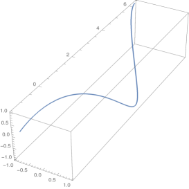
Figure 1. Circular Helix $:\left(\sin\frac{s}{\sqrt{2}},\frac{s}{\sqrt{2}},\cos\frac{s}{\sqrt{2}}\right).$

Example 3.5.

Suppose a curve $\varphi$ be parameterized as

(3.17) $$\varphi(s)=\left(\sin\frac{s}{\sqrt{2}},\frac{s}{\sqrt{2}},\cos\frac{s}{\sqrt{2}}\right).$$

The Frenet frame vectors $\{{\bf t,n,b}\}$ of (3.17) are given by

$${\bf t} = \left(\frac{1}{\sqrt{2}}\cos\frac{s}{\sqrt{2}},\frac{1}{\sqrt{2}},-\frac{1}{\sqrt{2}}\sin\frac{s}{\sqrt{2}}\right).$$

$${\bf n} = \left(-\sin\frac{s}{\sqrt{2}},0,-\cos\frac{s}{\sqrt{2}}\right).$$

$${\bf b} = \left(-\frac{1}{\sqrt{2}}\cos\frac{1}{\sqrt{2}},\frac{1}{\sqrt{2}},\frac{1}{\sqrt{2}}\sin\frac{1}{\sqrt{2}}s\right).$$

Also the curvature and torsion is given by

(3.18) $$\kappa(s)=\frac{1}{2},\quad\tau(s)=\frac{1}{2}.$$

Therefore the modified orthogonal frame vectors are given by

$$T(s) = {\bf t}=\left(\frac{1}{\sqrt{2}}\cos\frac{s}{\sqrt{2}},\frac{1}{\sqrt{2}},-\frac{1}{\sqrt{2}}\sin\frac{s}{\sqrt{2}}\right).$$

$$N(s) = \kappa{\bf n}=\left(-\frac{1}{2}\sin\frac{s}{\sqrt{2}},0,-\frac{1}{2}\cos\frac{s}{\sqrt{2}}\right).$$

$$B(s) = \kappa{\bf b}=\left(-\frac{1}{2\sqrt{2}}\cos\frac{s}{\sqrt{2}},\frac{1}{2\sqrt{2}},\frac{1}{2\sqrt{2}}\sin\frac{s}{\sqrt{2}}\right).$$

From the above frame vectors and (3.18), we see that $\varphi$ is arc length parameterized and a helix, respectively. Substituting the above quantities in (3.3), we see that equality in (3.2) is satisfied.

The higher derivative of $T(s)$ are given by

(3.22) $$\left\{\begin{array}[]{c}T^{\prime}(s)=\left(-\frac{1}{2}\sin\frac{s}{\sqrt{2}},0,-\frac{1}{2}\cos\frac{s}{\sqrt{2}}\right)\\ T^{\prime\prime}(s)=\left(-\frac{1}{2\sqrt{2}}\cos\frac{s}{\sqrt{2}},0,\frac{1}{2\sqrt{2}}\sin\frac{s}{\sqrt{2}}\right)\\ T^{\prime\prime\prime}(s)=\left(\frac{1}{4}\sin\frac{s}{\sqrt{2}},0,\frac{1}{4}\cos\frac{s}{\sqrt{2}}\right).\end{array}\right.$$

From (3.22), it is easy to verify (3.15).

Example 3.6.

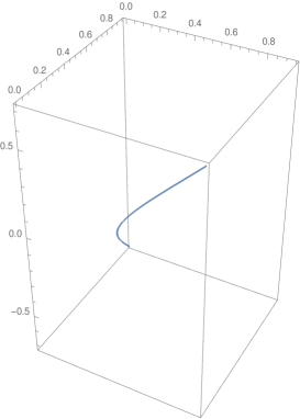
Figure 2. General Helix$:\left(\frac{\left(1+s\right)^{\frac{3}{2}}}{3},\frac{\left(1-s\right)^{\frac{3}{2}}}{3},\frac{s}{\sqrt{2}}\right).$

Let us consider a curve parameterized as

(3.23) $$\psi(s)=\left(\frac{\left(1+s\right)^{\frac{3}{2}}}{3},\frac{\left(1-s\right)^{\frac{3}{2}}}{3},\frac{s}{\sqrt{2}}\right),$$

where $-1<s<1$. The Frenet frame vectors $\{{\bf t,n,b}\}$ of (3.23) are found as:

$$\left\{\begin{array}[]{c}{\bf t}=\frac{1}{2}\left(\sqrt{1+s},-\sqrt{1-s},\sqrt{2}\right)\\ {\bf n}=\frac{1}{\sqrt{2}}\left(\sqrt{1-s},\sqrt{1+s},0\right)\\ {\bf b}={\bf t}\times{\bf n}=\frac{1}{2}\left(-\sqrt{1+s},\sqrt{1-s},\frac{\sqrt{2}}{2}\right)\end{array}\right.$$

and $\kappa=\tau=\frac{1}{\sqrt{8\left(1-s^{2}\right)}}.$

Therefore the modified orthogonal frame vectors are given by

$$T = {\bf t}=\left(\frac{\sqrt{1+s}}{2},-\frac{\sqrt{1-s}}{2},\frac{\sqrt{2}}{2}\right).$$

$$N = \kappa{\bf n}=\frac{1}{4}\left(\frac{1}{\sqrt{1+s}},\frac{1}{\sqrt{1-s}},0\right).$$

$$B = \kappa{\bf b}=\frac{1}{4\sqrt{2}}\left(-\frac{1}{\sqrt{1-s}},\frac{1}{\sqrt{1+s}},\frac{\sqrt{2}}{\sqrt{1-s^{2}}}\right).$$

Also, one can easily find

$$\dfrac{d\psi}{ds} = \mathrm{T}=\frac{1}{2}\allowbreak\left(\sqrt{1+s},-\sqrt{1-s},\sqrt{2}\right)$$

$$\dfrac{d^{2}\psi}{ds^{2}} = T^{\prime}=\frac{1}{4}\left(\frac{1}{\sqrt{1+s}},\frac{1}{\sqrt{1-s}},0\right)$$

$$\dfrac{d^{3}\psi}{ds^{3}} = T^{\prime\prime}=\frac{1}{8}\left(-\frac{1}{\left(1+s\right)^{\frac{3}{2}}},\frac{1}{\left(1-s\right)^{\frac{3}{2}}},0\right)$$

$$\dfrac{d^{4}\psi}{ds^{4}} = T^{\prime\prime\prime}=\frac{3}{16}\left(\frac{1}{\left(1+s\right)^{\frac{5}{2}}},\frac{1}{\left(1-s\right)^{\frac{5}{2}}},0\right)$$

Hence $\det(T^{\prime},T^{\prime\prime},T^{\prime\prime\prime})\$is zero. This verifies (3.15). Again substituting the required quantities in (3.3), equation (3.2) is a straightforward verification.

Theorem 3.7.

Let $\psi:I\rightarrow E^{3}$ be a unit speed curve in $E^{3}$ such that the curvature and torsion of the curve is a non-zero constant and non-constant, respectively. Then $\psi$ is a slant helix according to modified orthogonal frame if and only if the function

(3.25) $$\frac{\tau^{\prime}}{\left(\kappa^{2}+\tau^{2}\right)^{\frac{3}{2}}}$$

is constant.

Proof.

Let $\psi$ be the given unit speed curve in $E^{3}$. Let $U$ be the vector field such that the function $\left\langle N(s),U\right\rangle=c$ is constant. There exist smooth functions $a$ and $b$ such that

(3.26) $$U=a(s)T(s)+cN(s)+b(s)B(s),\ \ s\in I.$$

As $U$ is constant, a differentiation of (3.26) together (2.3) gives

(3.27) $$\left\{\begin{array}[]{c}a^{\prime}-c\kappa^{2}=0\\ a-b\tau\ \ =0\\ b^{\prime}+c\tau=0\end{array}\right.$$

From the second equation in (3.27), we get

(3.28) $$a=\tau b.$$

Moreover, since $U$ is a constant vector, we have

(3.29) $$\left\langle U,U\right\rangle=a^{2}+c^{2}\kappa^{2}+b\kappa^{2}=\textrm{constant}\text{.}$$

We point out that this constraint, together with the second and third equation of (3.27) is equivalent to the very system (3.27). Combining (3.27) and (3.29), let $m$ be the constant given by

$$b^{2}\left(\kappa^{2}+\tau^{2}\right)=\text{constant}-c^{2}\kappa^{2}=m^{2}.$$

This gives

$$b=\pm\frac{m}{\sqrt{\kappa^{2}+\tau^{2}}}.$$

The third equation in (3.27) yields

$$\frac{d}{ds}\left(\pm\frac{m}{\sqrt{\kappa^{2}+\tau^{2}}}\right)=c\tau$$

on $I$. This can be written as

$$\pm\frac{c}{m}=\frac{\tau^{{}^{\prime}}}{\left(\kappa^{2}+\tau^{2}\right)^{\frac{3}{2}}},\ \ \ \ \ \ \ \ \ \$$

which proves (3.25). Conversely, assume that the condition (3.25) is satisfied. In order to simplify the computations, we assume that the function in (3.25) is a constant, namely $c$ (the other case is analogous). Define

(3.30) $$U=\frac{m\tau}{\sqrt{\kappa^{2}+\tau^{2}}}T(s)+\frac{m}{\sqrt{\kappa^{2}+\tau^{2}}}B(s)+cN(s),\ \ s\in I.$$

A differentiation of (3.30) together with the modified orthogonal frame gives

$$U^{{}^{\prime}}=\dfrac{m\tau^{\prime}\kappa^{2}}{\left(\kappa^{2}+\tau^{2}\right)^{\frac{3}{2}}}T(s)-\dfrac{m\tau\tau^{\prime}}{\left(\kappa^{2}+\tau^{2}\right)^{\frac{3}{2}}}B(s)+\dfrac{m\tau}{\sqrt{\kappa^{2}+\tau^{2}}}N(s)$$

$$+\dfrac{m}{\sqrt{\kappa^{2}+\tau^{2}}}\left(-\tau N(s)\right)+\dfrac{m\tau^{\prime}}{\left(\kappa^{2}+\tau^{2}\right)^{3/2}}\left(-\kappa^{2}T(s)+\underbrace{\frac{\kappa^{\prime}}{\kappa}N}_{0}+\tau B(s)\right)=0$$

that is, $U$ is a constant vector. On the other hand,

$$\left\langle N(s),U\right\rangle=\left\langle N(s),\frac{m\tau}{\sqrt{\kappa^{2}+\tau^{2}}}T(s)+cN(s)+\frac{m}{\sqrt{\kappa^{2}+\tau^{2}}}B(s)\right\rangle=c.$$

This means that $\psi$ is a slant helix.

Remark 3.8.

For $\kappa=1$, we see that with respect to the modified orthogonal frame, the condition for slant helix in (3.25) is equal to the condition for slant helix with respect to Frenet-Serret frame in (1.1).

Example 3.9.

Salkowski [18] introduced a family of curves with constant curvature but non-constant torsion and called them as Salkowski curves. Later, Monterde [13] characterized Salkowski curves as the space curves with constant curvature and whose normal vector makes a constant angle with a fixed line. Thus, we can give Salkowski curves as striking example of slant helices.

∎

4. Bertrand curves with modified orthogonal frame

Definition 4.1.

Let $\varphi$ and $\psi$ be two curves with non-vanishing curvatures and torsions and $N_{\varphi}$ and $N_{\psi}$ are normals of $\varphi$ and $\psi$, respectively. If $N_{\varphi}$ and $N_{\psi}$ are parallel, then $\left(\varphi\ ,\psi\right)$ is called Bertrand pair [6].

From the definition of Bertrand pair $\left(\varphi(s)\ ,\psi(s^{\ast})\right)$, there is a functional relation $s^{\ast}=s^{\ast}(s)$ such that

$$\delta^{\ast}(s^{\ast}(s))=\delta(s).$$

Let $\left(\varphi\ ,\psi\right)$ be a Bertrand pair, we can write

(4.1) $$\psi(s)=\varphi(s)+\delta(s)N_{\varphi}(s).$$

Theorem 4.2.

The distance between the corresponding points of a Bertrand pair $\left(C_{\varphi},C_{\psi}\right)$ with respect to the modified orthogonal frame is constant.

Proof.

Let $C_{\varphi}$ and $C_{\psi}$ be given $\varphi(s)$ and $\psi(s)$, respectively. Using (4.1), we can write

$$\psi=\varphi+\delta N_{\varphi}.$$

Differentiating, and using modified orthogonal frame, we obtain

(4.2) $$\psi^{\prime}(s)=\left(1-\delta\kappa_{\varphi}^{2}\right)T_{\varphi}+\left(\delta^{\prime}+\frac{\delta\kappa_{\varphi}^{\prime}}{\kappa_{\varphi}}\right)N_{\varphi}+\delta\tau_{\varphi}B_{\varphi}.$$

Taking the inner product (4.2) with $N_{\varphi}$, and using $N_{\varphi}\parallel N_{\psi}$, we obtain

$$\left\langle N_{\varphi},\psi^{\prime}(s)\right\rangle=\delta^{\prime}+\frac{\delta\kappa_{\varphi}^{\prime}}{\kappa_{\varphi}}=0.$$

This implies

(4.3) $$-\frac{\delta^{\prime}}{\delta}=\frac{\kappa_{\varphi}^{\prime}}{\kappa_{\varphi}}.$$

Integrating (4.3), we get

(4.4) $$\delta(s)=\frac{c}{\kappa_{\varphi}(s)},$$

where $c$ a real number except zero, Therefore

$$\left\|\psi-\varphi(s)\right\|=\left\|\frac{c}{\kappa_{\varphi}(s)}N_{\varphi}(s)\right\|=\left|c\right|\left|\frac{1}{\kappa_{\varphi}}\right|\left|\kappa_{\varphi}\right|=\left|c\right|.$$

∎

Lemma 4.3.

The angle between tangent lines of a Bertran pair $(\varphi,\psi)$ is constant.

Proof.

Differentiaiting $\left\langle T_{\psi},T_{\varphi}\right\rangle$, we get

$$\frac{d}{ds}\left\langle T_{\psi},T_{\varphi}\right\rangle=\left\langle T_{\psi},N_{\varphi}\right\rangle+\left\langle T_{\psi},N_{\varphi}\right\rangle.$$

Since $\frac{N_{\psi}}{\kappa_{\psi}}=\pm\frac{N_{\varphi}}{\kappa_{\varphi}},$ $\left\langle N_{\psi},T_{\varphi}\right\rangle=0$ and $\left\langle N_{\varphi},T_{\psi}\right\rangle=0$ . Thus we get $\frac{d}{ds}\left\langle T_{\varphi},T_{\psi}\right\rangle=0$ and so $\left\langle T_{\varphi},T_{\psi}\right\rangle=$constant. ∎

Theorem 4.4.

A pair of curves $(C_{\varphi},C_{\psi})$ with $\tau_{\varphi}\neq 0$ is a Bertrand pair if and only if

(4.5) $$c\kappa_{\varphi}+ac\tau_{\varphi}=1,\text{ }$$

where $a=\cot\theta$ and $c=$constant.

Proof.

Suppose $(C_{\varphi}:\varphi,C_{\psi}:\psi)$ be a Bertrand pair with $\tau_{\varphi}\neq 0$. Let the modified orthogonal frames of $\varphi(s)$ and $\psi(s)$ are given by

$$\left\{T_{\varphi}={\bf t}_{\varphi},N_{\varphi}=\kappa_{\varphi}{\bf n}_{\varphi},B_{\varphi}=\kappa_{\varphi}{\bf b}_{\varphi}\right\},\left\{T_{\psi}={\bf t}_{\psi},N_{\psi}=\kappa_{\psi}{\bf n}_{\psi},B_{\psi}=\kappa_{\psi}{\bf b}_{\psi}\right\},$$

respectively. From Lemma 4.3, we know that the angle $\theta$ between $T_{\varphi}$ and $T_{\psi}$ is constant. Thus, we may write

(4.6) $$T_{\psi}=\cos\theta T_{\varphi}+\frac{\sin\theta}{\kappa_{\varphi}}B_{\varphi}.$$

Using (4.3) and (4.4) in (4.2), we get

(4.7) $$\psi^{\prime}(s)=\left(1-c\kappa_{\varphi}\right)T_{\varphi}+\frac{c\tau_{\varphi}}{\kappa_{\varphi}}B_{\varphi}.$$

From (4.6) and (4.7), we obtain

$$\frac{1-c\kappa_{\varphi}}{\cos\theta}=\frac{\frac{c\tau_{\varphi}}{\kappa_{\varphi}}}{\frac{\sin\theta}{\kappa_{\varphi}}}$$

or

(4.8) $$c\kappa_{\varphi}+ac\tau_{\varphi}=1.$$

Conversly, suppose $C_{\varphi}$ be a curve satisfying $c\kappa_{\varphi}+ac\tau_{\varphi}=1$ and $\tau_{\varphi}\neq 0$. Define another curve $C_{\psi}$ as:

$$\psi(s)=\varphi(s)+\delta(s)N_{\varphi}(s).$$

We shall prove that $C_{\varphi}$ and $C_{\psi}$ are Bertrand mates. From (4.7), we know

(4.9) $$\psi^{\prime}(s)=\left(1-c\kappa_{\varphi}\right)T_{\varphi}+\frac{c\tau_{\varphi}}{\kappa_{\varphi}}B_{\varphi}.$$

Using the given condition in (4.9), we obtain

$$\psi^{\prime}(s)=ac\tau_{\varphi}T_{\varphi}+\frac{c\tau_{\varphi}}{\kappa_{\varphi}}B_{\varphi}=c\left(aT_{\varphi}+\frac{B_{\varphi}}{\kappa_{\varphi}}\right)\tau_{\varphi}\text{.}$$

Hence the tangent vector to $C_{\psi}$ is given by

(4.10) $$T_{\psi}=\frac{\psi^{\prime}(s)}{\left\|\psi^{\prime}(s)\right\|}=\frac{c\tau_{\varphi}}{\left|c\tau_{\varphi}\right|}\frac{\left(aT_{\varphi}+\frac{B_{\varphi}}{\kappa_{\varphi}}\right)}{\sqrt{a^{2}+1}}=\pm\frac{aT_{\varphi}+\frac{B_{\varphi}}{\kappa_{\varphi}}}{\sqrt{a^{2}+1}};a=const.$$

Differentiation (4.10) with respect to $s^{\ast}$, we get

$$\frac{dT_{\psi}}{ds^{\ast}}=\pm\frac{1}{\sqrt{a^{2}+1}}\left\{aN_{\varphi}-\frac{\kappa_{\varphi}^{\prime}}{\kappa_{\varphi}^{2}}B_{\varphi}+\frac{1}{\kappa_{\varphi}}\left(-\tau_{\varphi}N_{\varphi}+\frac{\kappa_{\varphi}^{\prime}}{\kappa_{\varphi}}B_{\varphi}\right)\right\}\frac{ds}{ds^{\ast}}.$$

This implies that

$$N_{\psi}=\pm\frac{a-\frac{\tau_{\varphi}}{\kappa_{\varphi}}}{\sqrt{a^{2}+1}}\frac{ds}{ds^{\ast}}N_{\varphi}.$$

or

(4.11) $$\frac{N_{\psi}}{\kappa_{\psi}}=\pm\frac{a-\frac{\tau_{\varphi}}{\kappa_{\varphi}}}{\sqrt{a^{2}+1}}\frac{ds}{ds^{\ast}}\frac{\kappa_{\varphi}}{\kappa_{\psi}}\frac{N_{\varphi}}{\kappa_{\varphi}}.$$

Since $\frac{N_{\psi}}{\kappa_{\psi}}\textrm{ and }\pm\frac{N_{\varphi}}{\kappa_{\varphi}}$ are unit vectors, from (4.11), we have

$$\frac{ds^{\ast}}{ds}=\frac{\kappa_{\varphi}}{\kappa_{\psi}}\frac{a-\frac{\tau_{\varphi}}{\kappa_{\varphi}}}{\sqrt{a^{2}+1}}$$

and

$$\frac{N_{\psi}}{\kappa_{\psi}}=\pm\frac{N_{\varphi}}{\kappa_{\varphi}}.$$

This completes the proof. ∎

Theorem 4.5.

Let $(C_{\varphi},C_{\psi})\$be a Bertrand mate in Euclidean 3-space $E^{3}$ according to the modified orthogonal frame, then the following identities hold:

(4.14) $$\left\{\begin{array}[]{c}\kappa_{\varphi}=\frac{c\kappa_{\psi}+\sin^{2}\theta}{c\left(1+c\kappa_{\psi}\right)}\vspace{.2cm}\\ \tau_{\varphi}\tau_{\psi}=\left(\frac{\sin\theta}{c}\right)^{2}>0.\end{array}\right.$$

Proof.

From (4.6) and (4.7), we can write respectively,

(4.15) $$\left\{\begin{array}[]{c}\dfrac{1-c\kappa_{\varphi}}{\cos\theta}=\dfrac{ds^{\ast}}{ds}\Rightarrow\dfrac{ds^{\ast}}{ds}\cos\theta=1-c\kappa_{\varphi}\\ \dfrac{c\dfrac{\tau_{\varphi}}{\kappa_{\varphi}}}{\frac{\sin\theta}{\kappa_{\varphi}}}=\dfrac{ds^{\ast}}{ds}\Rightarrow\dfrac{ds^{\ast}}{ds}\sin\theta=c\tau_{\varphi}.\end{array}\right.$$

Interchanging the roles of $\varphi$ and $\psi$, thus $(\psi,\varphi)$ is also a Bertrand mate and in this case, $\delta$ and $\theta$ are replaced with $-\delta$ and $-\theta,$ respectively. Hence we can write as

(4.16) $$\left\{\begin{array}[]{c}\dfrac{ds}{ds^{\ast}}\cos\theta=1+c\kappa_{\psi}\\ \dfrac{ds}{ds^{\ast}}\sin\theta=c\tau_{\psi}.\end{array}\right.$$

By multiplying the first parts of (4.15) and (4.16), we get

$$\cos^{2}\theta=\left(1-c\kappa_{\varphi}\right)\left(1+c\kappa_{\psi}\right)$$

or

(4.17) $$\kappa_{\varphi}=\frac{c\kappa_{\psi}+\sin^{2}\theta}{c\left(1+c\kappa_{\psi}\right)}.\text{ }$$

Now multiplying the second parts of (4.15) and (4.16), we get

(4.18) $$\sin^{2}\theta=c^{2}\left(\tau_{\varphi}\tau_{\psi}\right).$$

From above equation, we see that

$$\tau_{\varphi}\tau_{\psi}>0.$$

∎

Example 4.6.

Let $\varphi$ be a curve parameterized by

(4.19) $$\varphi(s)=\left(\frac{1}{2\sqrt{2}}\sin 2s,\frac{1}{2\sqrt{2}}\cos 2s,\frac{s}{\sqrt{2}}\right).$$

The modified orthogonal frame vectors for (4.19) are given by

(4.20) $$T_{\varphi} = \left(\frac{1}{\sqrt{2}}\cos 2s,-\frac{1}{\sqrt{2}}\sin 2s,\frac{1}{\sqrt{2}}\right).$$

(4.21) $$N_{\varphi} = \left(-\sqrt{2}\sin 2s,-\sqrt{2}\cos 2s,0\right).$$

(4.22) $$B_{\varphi} = \left(-2\sin 2s,-2\cos 2s,0\right).$$

From above, we see that $\varphi$ is parameterized by arc length. Also, the curvature and torsion is given by:

$$\kappa_{\varphi}=\sqrt{2},\quad\tau_{\varphi}=-\sqrt{2}.$$

Now for $c=\frac{1}{\sqrt{2}}$, with the help of (4.1), we can construct a curve $\psi$ parameterized as

(4.23) $$\psi(s)=\left(-\frac{1}{2\sqrt{2}}\sin 2s,-\frac{1}{2\sqrt{2}}\cos 2s,\frac{s}{\sqrt{2}}\right).$$

The modified orthogonal frame vectors of (4.23) are found as

(4.24) $$T_{\psi} = \left(-\frac{1}{\sqrt{2}}\cos 2s,\frac{1}{\sqrt{2}}\sin 2s,\frac{1}{\sqrt{2}}\right).$$

(4.25) $$N_{\psi} = \left(\sqrt{2}\sin 2s,\sqrt{2}\cos 2s,0\right).$$

(4.26) $$B_{\psi} = \left(-\cos 2s,\sin 2s,-1\right).$$

From (4.21) and (4.25), we see that $(\varphi,\psi)$ is a Bertrand pair. The curvature and the torsion of $\psi(s)$ are given by

$$\kappa_{\psi}=\sqrt{2},\quad\tau_{\psi}=-\sqrt{2}.$$

From (4.20) and (4.24), we have $\theta=\frac{\pi}{2}$. Hence (4.5) is straightforward. Again substituting the required quantities, the identities in (4.14) are direct verifications.

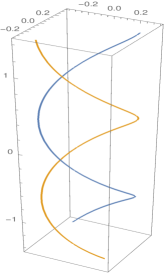
Figure 3. Bertrand pair $(\varphi,\psi)$

Theorem 4.7.

Suppose there exists a one-one relation between the points of the curves $C_{\varphi}$ and $C_{\psi}$, such that at the corresponding points $P_{\varphi}$ on $C_{\varphi}$ and $P_{\psi}$ on $C_{\psi}:$
(a) $\kappa_{\varphi}$ is constant.
(b) $\tau_{\psi}$ is constant.
(c) $T_{\varphi}$ is parallel to $T_{\psi}$,
then the curve $C$ generated by $P$ that divides the segment $P_{\varphi}P_{\psi}$ in ratio $h:1$ is a Bertrand curve.

Proof.

Let $\alpha(s),$ $\alpha_{\varphi}(s),$ $\alpha_{\psi}(s)$ be the coordinate vectors at the points $P$, $P_{\varphi}$, $P_{\psi}$ on the curves $C$, $C_{\varphi}$, $C_{\psi}$ respectively. Then from a convex combination of points $P_{\varphi}$ and $P_{\psi}$ , the equation of point $P$ is

(4.27) $$\alpha(s)=h\alpha_{\varphi}(s)+(1-h)\alpha_{\psi}(s),\,\,h\,\in R,h\,\in\left[0,1\right].\$$

Differentiating (4.27) with respect to $s$ and using the hypothesis, i.e., $T_{\varphi}=T_{\psi}\,,\,$we find

(4.28) $$\,\,\,Tds=hT_{\varphi}ds_{\varphi}+(1-h)T_{\psi}ds_{\psi}=\left[hds_{\varphi}+(1-h)ds_{\psi}\right]T_{\varphi}$$

(4.29) $$T=T_{\varphi}=T_{\psi}$$

(4.30) $$h\frac{ds_{\varphi}}{ds}+(1-h)\frac{ds_{\psi}}{ds}=1.$$

Similary, by differentiating (4.29), we obtain

(4.31) $$Nds=N_{\varphi}ds_{\varphi}=N_{\psi}ds_{\psi},\text{ }$$

(4.32) $$\kappa ds=\kappa_{\varphi}ds_{\varphi}=\kappa_{\psi}ds_{\psi},$$

and

(4.33) $$\frac{ds_{\varphi}}{ds}=\frac{\kappa}{\kappa_{\varphi}}.$$

(4.34) $$\frac{N}{\kappa}=\frac{N_{\varphi}}{\kappa_{\varphi}}=\frac{N_{\psi}}{\kappa_{\psi}}.$$

From the vector product of (4.29) and (4.34), we have

(4.35) $$\frac{B}{\kappa}=\frac{B_{\varphi}}{\kappa_{\varphi}}=\frac{B_{\psi}}{\kappa_{\psi}}.$$

Differentiating (4.35) and using (4.29),(4.34), we get

(4.36) $$\tau\frac{N}{\kappa}=\tau_{\psi}\frac{N_{\psi}}{\kappa_{\psi}}\frac{ds_{\psi}}{ds}$$

and

(4.37) $$\frac{ds_{\psi}}{ds}=\frac{\tau}{\tau_{\psi}}.$$

By inserting (4.33) and (4.37) in (4.30), we get

$$\left(\frac{h}{\kappa_{\varphi}}\right)\kappa+\left(\frac{1-h}{\tau_{\psi}}\right)\tau=1;\kappa_{\varphi}\neq 0,\tau_{\psi}\neq 0,$$

which is the desired result, since $h,\kappa_{\varphi},\tau_{\psi}$ are constant. ∎

Theorem 4.8.

If the condition (c) in Theorem 4.7 is modified so that at the corresponding points $P_{\varphi}$ and $\ P_{\psi}$ the binormals $B_{\varphi}$ and $B_{\psi}$ are parallel, then the curve $C$ is a Bertrand curve.

Proof.

Since $\dfrac{B_{\varphi}}{\kappa_{\varphi}}=\dfrac{B_{\psi}}{\kappa_{\psi}}$, similar as in (4.36) and (4.37), we obtain

(4.38) $$\frac{N_{\varphi}}{\kappa_{\varphi}}=\frac{\tau_{\psi}}{\tau_{\varphi}}\frac{ds_{\psi}}{ds_{\varphi}}\frac{N_{\psi}}{\kappa_{\psi}}.$$

and

(4.39) $$\frac{ds_{\psi}}{ds_{\varphi}}=\frac{\tau_{\varphi}}{\tau_{\psi}}.$$

Using (4.39), we can rewrite (4.38) as

$$\frac{N_{\varphi}}{\kappa_{\varphi}}=\frac{N_{\psi}}{\kappa_{\psi}}.$$

Thus, we have

$$T_{\varphi}=\dfrac{N_{\varphi}}{\kappa_{\varphi}}\times\dfrac{B_{\varphi}}{\kappa_{\varphi}}=\dfrac{1}{\kappa_{\varphi}^{2}}\left(\dfrac{\kappa_{\varphi}}{\kappa_{\psi}}N_{\psi}\times\dfrac{\kappa_{\varphi}}{\kappa_{\psi}}B_{\psi}\right)=\frac{N_{\psi}}{\kappa_{\psi}}\times\frac{B_{\psi}}{\kappa_{\psi}}=T_{\psi}.$$

Therefore $T_{\varphi}$ is parallel to $T_{\psi}$, so that by Theorem 4.7, $C$ is a Bertrand curve . ∎

Theorem 4.9.

If the condition (c) in Theorem 4.7 is modified so that at the corresponding points $P_{\varphi}$ and $\ P_{\psi}$ the tangent $T_{\varphi}$ at $P_{\varphi}$ is parallel to the binormal $B_{\psi}$ at $P_{\psi}$, then the curve $C$ is a Bertrand curve.

Proof.

Since $T_{\varphi}=\dfrac{B_{\psi}}{\kappa_{\psi}}$, it follow that

(4.40) $$N_{\varphi}=-\frac{\tau_{\psi}}{\kappa_{\psi}}\frac{ds_{\psi}}{ds_{\varphi}}N_{\psi}.\ \ \ \ \ \ \ \ \ \ \ \ \ \ \ \ \$$

Hence $N_{\varphi}$ is parallel to $N_{\psi}$ and since $\frac{N_{\varphi}}{\kappa_{\varphi}}$ and $\frac{N_{\psi}}{\kappa_{\psi}}$ are unit vectors,

(4.41) $$\frac{N_{\varphi}}{\kappa_{\varphi}}=\pm\frac{N_{\psi}}{\kappa_{\psi}}$$

From (4.40) and (4.41), we get

(4.42) $$\frac{ds_{\psi}}{ds_{\varphi}}=-\frac{\kappa_{\varphi}}{\tau_{\psi}}\ .$$

Moreover since

$$B_{\varphi}=T_{\varphi}\times N_{\varphi}=\dfrac{B_{\psi}}{\kappa_{\psi}}\times\frac{\kappa_{\varphi}}{\kappa_{\psi}}N_{\psi}=\frac{\kappa_{\varphi}}{\kappa_{\psi}^{2}}\left(B_{\psi}\times N_{\psi}\right)=\frac{\kappa_{\varphi}\kappa_{\psi}^{2}}{\kappa_{\psi}^{2}}\left(-T_{\psi}\right)=-\kappa_{\varphi}T_{\psi}\text{,}$$

we get

$$T_{\psi}=-\frac{B_{\varphi}}{\kappa_{\varphi}}.$$

Let  $R,$ $R_{\varphi},$ $R_{\psi}$ be the coordinate vectors at the points $P$, $P_{\varphi}$, $P_{\psi}$ on the curves $C$, $C_{\varphi}$, $C_{\psi}$ respectively. Then

(4.43) $$R=hR_{\varphi}+(1-h)R_{\psi}.$$

By differentiating (4.43) with respect to $s$ and by (4.42), we have

(4.44) $$T=\left[hT_{\varphi}-\frac{\kappa_{\varphi}}{\tau_{\psi}}(1-h)T_{\psi}\right]\frac{ds_{\varphi}}{ds}.$$

Taking the norm of (4.44), we obtain

(4.45) $$\frac{ds_{\varphi}}{ds}=\frac{\tau_{\psi}}{\sqrt{h^{2}\tau_{\psi}^{2}+\kappa_{\varphi}^{2}(1-h)^{2}}}.$$

Thus with the help of (4.45), we can rewrite (4.44) as

$$T=\left[\frac{h\tau_{\psi}}{\sqrt{h^{2}\tau_{\psi}^{2}+\kappa_{\varphi}^{2}(1-h)^{2}}}\right]T_{\varphi}+\left[\frac{-(1-h)\kappa_{\varphi}}{\sqrt{h^{2}\tau_{\psi}^{2}+\kappa_{\varphi}^{2}(1-h)^{2}}}\right]T_{\psi}$$

or

(4.46) $$\ T=h_{\varphi}T_{\varphi}+h_{\psi}T_{\psi}\ ,\ \$$

where

$$h\frac{ds_{\varphi}}{ds} = \frac{h\,\,\tau_{\psi}}{\sqrt{h^{2}\tau_{\psi}^{2}+\kappa_{\varphi}^{2}(1-h)^{2}}}=h_{\varphi},\,\,h_{\varphi}=\text{constant}$$

$$(1-h)\frac{ds_{\psi}}{ds} = -\,\frac{\,\left(1-h\right)\kappa_{\varphi}}{\sqrt{h^{2}\tau_{\psi}^{2}+\kappa_{\varphi}^{2}(1-h)^{2}}}=h_{\psi},\ h_{\psi}=\text{constant}$$

Differentiating (4.46), one can easily get

(4.47) $$\frac{N}{\kappa}=h_{\varphi}\frac{ds_{\varphi}}{ds}\frac{N_{\varphi}}{\kappa_{\varphi}}+h_{\psi}\frac{ds_{\psi}}{ds}\frac{N_{\psi}}{\kappa_{\psi}}.$$

Hence

(4.48) $$\frac{N}{\kappa}=\frac{N_{\varphi}}{\kappa_{\varphi}}=\frac{N_{\psi}}{\kappa_{\psi}}$$

and

(4.49) $$\kappa=\kappa_{\varphi}h_{\varphi}\frac{ds_{\varphi}}{ds}+\kappa_{\psi}h_{\psi}\frac{ds_{\psi}}{ds}.$$

Using (4.46) and (4.48), we can find

(4.50) $$\frac{B}{\kappa}=h_{\varphi}\frac{B_{\varphi}}{\kappa_{\varphi}}+h_{\psi}\frac{B_{\psi}}{\kappa_{\psi}}.$$

Differentiating (4.50), we have

(4.51) $$\tau\frac{N}{\kappa}=h_{\varphi}\tau_{\varphi}\frac{ds_{\varphi}}{ds}\frac{N_{\varphi}}{\kappa_{\varphi}}+h_{\psi}\tau_{\psi}\frac{ds_{\psi}}{ds}\frac{N_{\psi}}{\kappa_{\psi}}.$$

Hence

(4.52) $$\tau=\tau_{\varphi}h_{\varphi}\frac{ds_{\varphi}}{ds}+\tau_{\psi}h_{\psi}\frac{ds_{\psi}}{ds}.$$

Using (4.38) and (4.39), we have

$$-\frac{\kappa_{\varphi}}{\tau_{\psi}}=\frac{ds_{\psi}}{ds_{\varphi}}=\frac{\tau_{\varphi}}{\kappa_{\psi}}\text{ }$$

and

(4.53) $$\frac{\tau_{\varphi}}{\kappa_{\varphi}}=-\frac{\kappa_{\psi}}{\tau_{\psi}}.$$

Assume that

$$M_{\varphi}=h_{\varphi}\frac{ds_{\varphi}}{ds},\ M_{\psi}=h_{\psi}\frac{ds_{\psi}}{ds},$$

then by (4.49),(4.52) and (4.53), we have

$$\frac{\kappa}{\tau_{\psi}M_{\psi}}+\frac{\tau}{\kappa_{\varphi}M_{\varphi}} = \frac{\kappa_{\varphi}M_{\varphi}+\kappa_{\psi}M_{\psi}}{\tau_{\psi}M_{\psi}}+\frac{\tau_{\varphi}M_{\varphi}+\tau_{\psi}M_{\psi}}{\kappa_{\varphi}M_{\varphi}}$$

$$= \frac{\kappa_{\varphi}}{\tau_{\psi}}\frac{M_{\varphi}}{M_{\psi}}+\underset{0}{\underbrace{\left(\frac{\kappa_{\psi}}{\tau_{\psi}}+\frac{\tau_{\varphi}}{\kappa_{\varphi}}\right)}}+\frac{\tau_{\psi}}{\kappa_{\varphi}}\frac{M_{\psi}}{M_{\varphi}}$$

$$= \frac{\kappa_{\varphi}}{\tau_{\psi}}\frac{M_{\varphi}}{M_{\psi}}+\frac{\tau_{\psi}}{\kappa_{\varphi}}\frac{M_{\psi}}{M_{\varphi}}=\text{constant.}$$

Since $\frac{\kappa_{\varphi}}{\tau_{\psi}}$ and $\ \frac{M_{\varphi}}{M_{\psi}}=\frac{h}{1-h}\frac{ds_{\psi}}{ds_{\varphi}}=\frac{h}{1-h}\frac{\kappa_{\varphi}}{\tau_{\psi}}$ are constant and this is the intrinsic equation of a Bertrand curve. ∎

5. Acknowledgment

The authors would like to thank all the anonymous referees for their valuable comments and suggestions which helped to improve this paper.

References

- [1] A. T. Ali, R. Lopez, Slant helices in Minkowski space , J. Korean Math. Soc., 48, 159-167, 2011.
- [2] H. Balgetir, M. Bektas, J. Inoguchi, J, Null Bertrand Curves in Minkowski 3-space and their Characterizations, Note di Matematica 23(1),7-13, 2004.
- [3] M. Barros, General helices and a theorem of Lancret, Proc. Amer. Math. Soc. 125 (5), 1503-1509, 1997.
- [4] J.M. Bertrand, Mémoire sur la théorie des courbes á double courbure. J. Math. Pures. Appl. 15, 332-350, 1850.
- [5] J.F. Burke, Bertrand Curves Associated with a Pair of Curves, Mathematics Magazine, 34(1), 60-62, 1960.
- [6] M.Do Carmo, Differential Geometry of Curves and Surfaces, Prentice-Hall, New Jersey, 1976.
- [7] N. Ekmekci, On General Helices and Submanifolds of an Indefinite-Riemann Manifold, An. Ştiint. Univ. Al. I. Cuza Iaşi Mat. (N.S.), 46(2), 263-270, 2000.
- [8] K. Ilarslan, Characterizations of Spacelike General Helices in Lorentzian Manifolds, Kragujevac J. Math., 25, 209-218, 2003.
- [9] S. Izumiya and N. Takeuchi, New special curves and developable surfaces, Turkish J. Math. 28, 153-163, 2004.
- [10] L. Kula, N. Ekmekçi, Y. Yaylı, K. Ilarslan, Characterizations of slant helices in Euclidean 3-space. Turk. J. Math., 34, 261-273, 2010.
- [11] L. Kula, Y. Yaylı, On slant helix and its spherical indicatrix. Applied Mathematics and Computation. 169(1), 600-607, 2005.
- [12] H. Matsuda, S.H. Yorozu, Notes on Bertrand Curves, Yokohama Mathematical Journal, 50, 41-58, 2003.
- [13] J. Monterde, Salkowski curves revisted: A family of curves with constant curvature and non-constant torsion, Comput. Aided Geom. Design, 26, 271-278, 2009.
- [14] A.W. Nutbourne, R.R. Martin, Differential Geometry Applied to the Design of Curves and Surfaces, ellis Horwood, Chichester, UK, 1988.
- [15] A.O. Ogrenmis, H. Oztekin, M. Ergut, Bertrand Curves in Galilean Space and Their Characterizations, Kragujevac J. Math. 32, 139-147, 2009.
- [16] A.O. Ogrenmis, M. Ergut, M. Bektas, On The Helices in The Galilean Space , Iranian J. of Sci. & Tech., Transaction A, Vol. 31(A2), 177-181, 2007.
- [17] H.B. Oztekin, M. Bektas, Representation formulae for Bertrand curves in the Minkowski 3-space, Scientia Magna, 6(1), 89-96, 2010.
- [18] E. Salkowski, Zur transformation von raumkurven, Mathematische Annalen, 66(4), 517-557, 1909.
- [19] T. Sasai. The Fundamental Theorem of Analytic Space Curves and Apparent Singularities of Fuchsian Differential Equations. Tohoku Math Journ., 36, 17-24, 1984.
- [20] W.K. Schief, On the integrability of Bertrand curves and Razzaboni surfaces, J. Geom. Phys., 45, 130-150, 2003.
- [21] D.J. Struik, Lectures on Classical Differential Geometry, 2nd edn. (Addison Wesley, Dover), 1988.
- [22] B. van-Brunt and K. Grant, Potential application of Weingarten surfaces in CADG, Part I: Weingarten surfaces and surface shape investigation, Comput. Aided Geom. Design, 13, 569-582, 1996.
- [23] D.W. Yoon, General Helices of AW(k)-Type in the Lie Group, Journal of Applied Mathematics, Article ID 535123, 10 pages,doi:10.1155/2012/535123,Volume 2012.