The rest-frame optical sizes of massive galaxies with suppressed star formation at $z\sim 4$

Abstract

We present the rest-frame optical sizes of massive quiescent galaxies (QGs) at $z\sim 4$ measured at $K^{\prime}$-band with the Infrared Camera and Spectrograph (IRCS) and adaptive optics facility, AO188, on the Subaru telescope. Based on a deep multi-wavelength catalog in the Subaru XMM-Newton Deep Survey Field (SXDS), covering a wide wavelength range from the $u$-band to the IRAC $8.0\mu m$ over 0.7 deg², we evaluate photometric redshift to identify massive ($M_{\star}\sim 10^{11}\ M_{\odot}$) galaxies with suppressed star formation. These galaxies show a prominent Balmer break feature at $z\sim 4$, suggestive of an evolved stellar population. We then conduct follow-up $K^{\prime}$-band imaging with adaptive optics for the five brightest galaxies ($K_{AB,total}=22.5\sim 23.4$). Compared to lower redshift ones, QGs at $z\sim 4$ have smaller physical sizes of effective radii $r_{eff}=0.2$ to $1.7$ kpc. The mean size measured by stacking the four brightest objects, a more robust measurement, is $r_{eff}=0.5\rm\ kpc$. This is the first measurement of the rest-frame optical sizes of QGs at $z\sim 4$. We evaluate the robustness of our size measurements using simulations and find that our size estimates are reasonably accurate with an expected systematic bias of $\sim 0.2$ kpc. If we account for the stellar mass evolution, massive QGs at $z\sim 4$ are likely to evolve into the most massive galaxies today. We find their size evolution with cosmic time in a form of $\log(r_{e}/{\rm kpc})=-0.56+1.91\log(t/\rm Gyr)$. Their size growth is proportional to the square of stellar mass, indicating the size-stellar mass growth driven by minor dry mergers.

1 Introduction

There is mounting evidence for the presence of massive galaxies with suppressed star formation at $z>2$ (e.g., Daddi et al. 2005; van Dokkum et al. 2008). These galaxies are known to be remarkably compact and dense compared to local ones (e.g., Trujillo et al. 2006; Toft et al. 2007; van Dokkum et al. 2008; van der Wel et al. 2014; Kubo et al. 2017). The size evolution of these massive quiescent galaxies (QGs) can be parameterized as $r\propto(1+z)^{\beta}$ where $\beta\sim-1.5$ which is steeper than $\beta\sim-1$ of star forming galaxies (SFGs; e.g., van der Wel et al. 2014; Shibuya et al. 2015).

The remarkable compactness and early formation of massive QGs pose a challenge to the standard picture of galaxy formation in which galaxies grow hierarchically and become more massive with time. Gas rich major mergers (e.g., Hopkins et al. 2008; Wellons et al. 2015) and infall of giant clumps formed via disk instability (e.g., Elmegreen et al. 2008; Dekel et al. 2009) can trigger nuclear starburst and increase the central density in galaxies to form a compact remnant. Discoveries of compact starburst galaxies at $z>2$ may support these scenarios (Toft et al., 2014; Barro et al., 2014; Ikarashi et al., 2015; Barro et al., 2016; Ikarashi et al., 2017; Barro et al., 2017; Gómez-Guijarro et al., 2018). On the other hand, massive QGs at high redshift need several to ten times growth in size but less growth in stellar mass to evolve into giant elliptical galaxies today. Dry minor mergers (e.g., Bezanson et al. 2009; Naab et al. 2009), adiabatic expansion (Fan et al., 2008; van Dokkum et al., 2014) and size evolution of newly quenched galaxies with redshift (Carollo et al., 2013; Poggianti et al., 2013; Belli et al., 2015) have been proposed as the driver of this steep size growth.

Now massive QGs at $z\sim 4$ are found photometrically (Straatman et al., 2014) and confirmed spectroscopically ($z_{spec}=3.717$; Glazebrook et al. 2017; Schreiber et al. 2018). The Hubble Space Telescope (HST) has been the main workhorse in the field of galaxy morphologies at high redshift, but it can not probe the rest-frame optical wavelength regime of galaxies at $z>3$ due to its wavelength cutoff of $\sim 1.7~{}\mu m$. In this study, we select galaxies with a prominent Balmer break feature at $z\sim 4$ photometrically from the Subaru XMM-Newton Deep Survey (SXDF; Furusawa et al. 2008) and investigate their rest-frame optical morphologies by the deep $K^{\prime}$-band images obtained with the adaptive optics (AO) on the Subaru Telescope.

This paper is organized as follows: in Section 2 we describe our sample selection of massive galaxies with suppressed star formation, in Section 3 we describe the observation and data reduction procedure, in Section 4 we describe the size measurement method and possible errors, and in Section 5 we show the results. We discuss the stellar mass surface density and size-stellar mass evolution of them in Section 6. Throughout the paper, we adopt a $\Lambda$CDM cosmology with $H_{0}=70$ km s^-1 Mpc^-1, $\Omega_{\Lambda}=0.7$ and $\Omega_{m}=0.3$, and magnitudes are given in the AB system.

2 Sample construction

2.1 Multi-band Catalog

We base our analysis on a multi-band photometric catalog in the Subaru XMM-Newton Deep Field (SXDF; Furusawa et al. 2008). SXDF has deep optical imaging from Suprime-Cam of the Subaru Telescope in $BVRiz$-bands (Furusawa et al., 2008). The UKIRT Infrared Deep Sky Survey (UKIDSS; Lawrence et al. 2007) is centered on the same field and we use the Data Release 10 to complement the optical data. Furthermore, the $u$-band photometry from CFHT Megacam and Spitzer photometry from the Spitzer UKIDSS Ultra Deep Survey (SpUDS; Dunlop et al. 2007) are available, allowing us to cover the entire optical and IR wavelengths up to $24\mu m$ over a wide area. It is an excellent field to search for faint, rare objects at high redshifts.

We first register all the optical images to the WCS grid of the UKIDSS images. The seeing is different from band to band, and we apply a Gaussian kernel to homogenize the seeing to $\sim 0.82$ arcsec. We run SExtractor (Bertin & Arnouts, 1996) on the $K$-band image to detect sources. We then measure sources in the other optical and nearIR bands using the dual image mode. We perform photometry within a circular aperture of 2.0 arcsec in all the bands. Because we miss a fraction of total light in this aperture, we measure the Kron fluxes of objects in the $K$-band and estimate the aperture correction, assuming the Kron flux is the total flux (here after we refer to the Kron magnitude as the total magnitude). We apply the aperture correction to the 2.0 arcsec aperture photometry in all the bands so that our photometry is closer to total light while keeping the accurate colors.

Because of the relatively large PSF sizes of the Spitzer/IRAC images, objects are often blended with nearby objects, and we choose to perform the Spitzer photometry separately from the optical-nearIR bands. We use T-PHOT (Merlin et al., 2015) version 1.5.11 to fit 2d profiles of objects in the IRAC images taking the object blending into account using the $K$-band image as a prior. For objects detected in the $K$-band high-resolution image (HRI), small image cutouts of the same region are generated in order to model the IRAC low-resolution image (LRI). The cutouts are convolved with a kernel constructed from LRI and HRI, both of which are constructed from point sources selected in HRI, to homogenize the PSF.　 Then, the optimization process is performed by scaling the fluxes of the objects of the PSF-matched HRI to match the LRI using the $\chi^{2}$ minimization technique. We process the IRAC images in all channels from 3.6$\mu$m to 8.0$\mu$m in the same way, and we use the total magnitude of each object from the best-fit model flux.

In the final catalog, we have about $10^{5}$ objects over $\sim 0.7$ deg² with coverage in all the filters. Table LABEL:tab:depth summarizes the depth in each band.

Table 1: $5\sigma$ limiting magnitudes within 2 arcsec apertures for each filter.

filter	instrument	depth
$u$	Megacam	26.8
$B$	Suprime-Cam	27.6
$V$	Suprime-Cam	27.3
$R$	Suprime-Cam	27.1
$i$	Suprime-Cam	27.0
$z$	Suprime-Cam	26.0
$J$	WFCAM	25.2
$H$	WFCAM	24.6
$K$	WFCAM	25.0
ch1	IRAC	24.8
ch2	IRAC	24.3
ch3	IRAC	22.6
ch4	IRAC	22.5

2.2 Target Selection

We run a custom photometric redshift code (Tanaka, 2015) on the multi-band catalog. This is a template-fitting code and we use templates generated using the Bruzual & Charlot (2003) stellar population synthesis code. We adopt the following assumptions in the models: exponentially declining star formation history, solar metallicity, Calzetti et al. (1994) attenuation curve, and Chabrier (2003) initial mass function (IMF). As we know the SFR and attenuation of each template, we add emission lines due to star formation using the emission line intensity ratios by Inoue (2011) (see Tanaka 2015 for details). The code infers redshifts and physical properties of galaxies such as stellar mass in a self-consistent manner and the uncertainties on the physical properties quoted in the paper have been estimated by marginalizing over all the other parameters, including redshift. As we have a large number of filters spanning a wide wavelength range, the data has a strong constraining power on the overall SED shapes. We therefore choose to apply flat priors in the fitting. We have confirmed that our results do not signifiantly change if we apply the full priors. Using some of the publicly available spectroscopic redshifts (Bradshaw et al. 2013; McLure et al. 2013, Simpson et al. in prep), we achieve a normalized dispersion of $\sigma(\Delta z/(1+z))=0.029$ and an outlier rate of 4.8%, where the outliers are defined in the conventional way (i.e., those with $|\Delta z/(1+z)|>0.15$; Tanaka et al. 2017). However, the spectroscopic sample is heterogeneous and the numbers here should not be over-interpreted.

We exclude objects with unreliable photo-$z$’s using the reduced chi-squares, $\chi_{\nu}>4$. Poor chi-squares are often due to poor photometry (e.g., halos around bright stars and object blending). For the purpose of this paper, we do not need a complete sample of evolved galaxies at high redshift and this cut does not introduce any bias. We then select galaxies at $3.5<z_{phot}<4.5$. Fig. 1 shows star formation rate (SFR) against stellar mass of the $z\sim 4$ galaxies. Both SFR and stellar mass are from the SED fit. There is a clear sequence of SFGs and also a population of massive galaxies with suppressed star formation. These two populations can be separated very well at specific SFR (sSFR) of $10^{-9.5}\rm yr^{-1}$. To be conservative, we choose galaxies whose $1\sigma$ upper limit of their sSFR is lower than $10^{-9.5}\rm yr^{-1}$ as the targets for the near-IR follow-up imaging with AO. The red filled points in Fig. 1 satisfy this condition. We note that there is some ambiguity in the definition of QGs in the literature, but when we refer to QGs in what follows, we mean galaxies with suppressed star formation as defined in Fig. 1. The $UVJ$ diagram is often used to define QGs, but it is tuned at $z\lesssim 2$ (Labbé et al., 2005; Williams et al., 2009) and is not clear whether it can be applied to $z\sim 4$ galaxies. For this reason, we adopt the sSFR-based definition.

In addition to the sSFR constraint, further practical constraints come from the location of tip-tilt stars for the AO-assisted observation. Since we need tip-tilt stars $R=16.5$ or brighter (for NGS mode, $R<19$ for LGS mode) for AO188, the available targets are further limited. We have conducted the near-IR follow-up imaging with AO for five of the brightest QGs with suitable tip-tilt stars as shown by the stars in Fig. 1 (here after ID1-5). Fig. 2 shows their SEDs. All of them are located around $z_{phot}\sim 4$. As can be seen, all the objects show a prominent Balmer break, indicative of an evolved stellar population. ID1 and ID2 have a faint UV continuum and are consistent with passively evolving galaxies (SED-based SFR is consistent with zero). The others have a brighter UV continuum, but the break feature is still prominent. To further characterize our targets, we compare the mean SEDs of SFGs with that of QGs in Fig. 3. SFGs have a very blue UV continuum with a strong Lyman break. On the other hand, the SEDs of our targets are clearly distinct; they have a suppressed UV continuum with a clear Balmer break. This break cannot be due to dust extinction because it does not introduce a sudden break at 3650Å while keeping the continuum at longer wavelengths blue. This is due to abundant A-type stars in these galaxies. The observed targets are consistent with the mean SED shown by the red shades and that suggests that they are representative of the evolved population around that redshift.

We note that a part of our survey area is observed in the Fourstar Galaxy Evolution survey (ZFOURGE) (Straatman et al., 2016). Straatman et al. (2014) select QGs at $z\sim 4$ using the rest-frame $UVJ$ colors and photometric redshifts from ZFOURGE. We briefly compare our sample of QGs with those in Straatman et al. (2014). We find that the QGs identified in SXDF (UDS) in Straatman et al. (2014) all satisfy sSFR$<10^{-9.5}\rm yr^{-1}$ based on our catalog. On the other hand, two of our targets, ID3 and ID5 are in the ZFOURGE field. ID3 is also identified as a QG in ZFOURGE, whereas ID5 is not. The rest-frame color of ID5 is $U-V=0.95\pm 0.04$ and $V-J=0.86\pm 0.02$ (Straatman et al., 2016), slightly bluer than the color criterion for QGs adopted in Straatman et al. (2014), but their SED fit suggests sSFR $<10^{-9.5}\rm yr^{-1}$ at $z_{\rm phot}\approx 4$, satisfying our criterion of QGs. Overall, our QG selection is broadly compatible with that of Straatman et al. (2014). It is noteworthy that, most of QGs in their sample are fainter than $K>23$. Thanks to the wider area coverage, most of our targets are brighter and better suited for detailed structural studies.

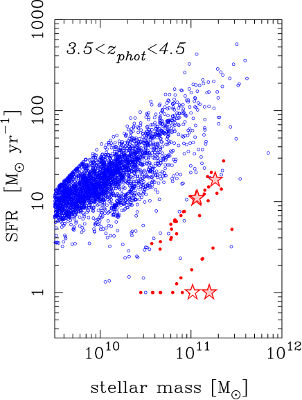
Figure 1: SFR v.s. stellar mass of galaxies at $z\sim 4$. The open circles are SFGs. The filled circles are QG candidates with a $1\sigma$ upper limit of the sSFR lower than $10^{-9.5}\rm\ yr^{-1}$. Objects with SFRs smaller than 1$\rm M_{\odot}\ yr^{-1}$ are shown at SFR=$1\rm M_{\odot}\ yr^{-1}$ only for illustrative purposes. The stars indicate the targets observed with IRCS+AO188 (see §3). The open star is ID3, the target also classified as quiescent by Straatman et al. (2014).

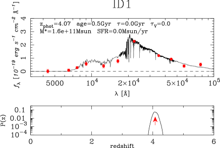
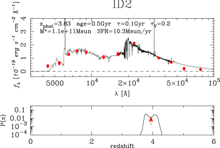
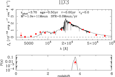
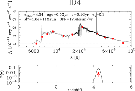
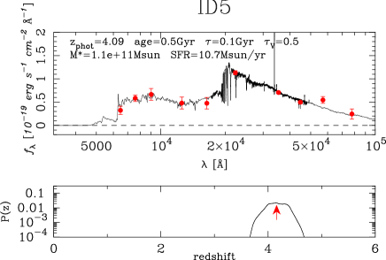
Figure 2: Top: The SEDs of our targets, ID1 to ID5. The spectrum is the best-fitting template spectrum and the points are the observed photometry. Some of the relevant quantities such as age and star formation timescale of the template are also indicated. Bottom: Redshift probability distribution function. The arrow shows the median redshift.

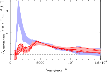
Figure 3: Rest-frame mean SEDs of SFGs (blue) and QGs (red) normalized in the $V$-band. The shaded areas encompass the 68 percentile of the distribution. The objects that we observed are shown as the solid lines. They show the prominent Balmer break.

3 Observation and data reduction

We observed the five targets selected in §2 with IRCS (Tokunaga et al., 1998; Kobayashi et al., 2000)+AO188 (Hayano et al., 2008, 2010) on the Subaru Telescope on the 25th and 26th of September 2016. We used the $K^{\prime}$ filter with the 52 mas pixel scale. The observing conditions were fair; the sky was clear on both nights with reasonably good seeing ($\sim 0.2$ arcsec with AO), though it fluctuated occasionally. We observed both in NGS and LGS modes due to occasional poor seeing and satellite crossings. We reject the worst $\sim 10$% of the bad seeing frames. After rejecting these bad PSF frames, the variation of PSF sizes of the frames on each target is less than 0.05 arcsec.

We reduced the data using the IRAF data reduction tasks following the data reduction manual for the IRCS. We first mask bad pixels and then apply the flat, which were constructed from dithered science exposures with objects masked out. The sky background is the median value in the whole area of each frame, $\sim 54$ arcsec on a side. We estimate the telescope offset between the pointing from the relative positions of bright stars within the field of view. Finally, we combine the frames with 3 sigma clipping.

Magnitude zero-points are calibrated by using the $K$-band images of UKIDSS. We estimate $K-K^{\prime}$ (i.e., WFCAM - IRCS) color as a function of $J-K$ color using the stellar library from Pickles (1998). We set the zero points of the IRCS-AO $K^{\prime}$-band images by matching the fluxes of bright ($K<21$) but not saturated stars with those measured on the UKIDSS $K$-band images after applying the $K-K^{\prime}$ color term. The $K-K^{\prime}$ colors of the stars used as the standard stars here range from $-0.12$ to $-0.10$. Since observing conditions were stable during the nights, we use the average of magnitude zero-points of each night, $25.41$ for 25th Sep (ID2 & 3) and $25.43$ for 26th Sep (ID1,4 & 5).

We summarize the details of the coadd images in Table 2. The total exposure time of each target ranges from 18 to 54 minutes. The FWHM PSF sizes measured on the PSF reference stars range from $0.15$ to $0.23$ arcsec.

Table 2: Summary of observations

ID	R.A.	Dec	EXPTIME	ZEROPOINT	depth	separation	FWHM PSF
	(h:m:s)	(d:m:s)	(min)	(mag)	(mag)	(arcsec)	(arcsec)
1	02:19:01.511	-05:18:29.07	33	$25.43$	24.7	72(33)	0.17
2	02:17:59.073	-05:09:39.89	18	$25.43$	24.6	53(34)	0.21
3	02:17:22.781	-05:17:33.34	35	$25.41$	24.9	48(16)	0.15
4	02:17:19.833	-04:43:34.75	43	$25.43$	25.0	41(38)	0.23
5	02:16:58.232	-05:08:35.21	54	$25.41$	25.0	37(13)	0.19

4 Size measurement

4.1 Flux completeness

We first examine the flux completeness of our targets on the IRCS-AO $K^{\prime}$-band images by comparing the flux measured on the IRCS-AO $K^{\prime}$-band and UKIDSS $K$-band images. The S/N on our $K^{\prime}$-band images are lower than that on the UKIDSS $K$-band images. Then if our targets have morphologies dominated by low-surface brightness components, large fraction of their fluxes detectable on the UKIDSS $K$-band images may go below the detection limit on our IRCS-AO $K^{\prime}$-band images. Also, the AO-corrected PSF tends to have an extended wing, which also introduces a diffuse component in the observed profiles. These effects can result in underestimated sizes and fluxes.

We compare the $K^{\prime}$-band total magnitudes measured on our IRCS-AO $K^{\prime}$-band ($K^{\prime}_{total,IRCS-AO}$) with the UKIDSS $K$-band magnitudes corrected of the $K-K^{\prime}$ color term using the best-fit SED model ($K^{\prime}_{total,synth}$) in order to evaluate the missing flux (Fig. 4 and Table 3). Overall, we tend to underestimate the fluxes in the IRCS-AO images as expected. For ID4 and ID5, we underestimate only by 10% and the missing light probably does not affect our size measurements significantly. However, we miss $25-50$% of the light for the other targets. Though a care is needed when interpreting individual galaxies, the stacked galaxy (open circle, see §4.4) does not show a significant amount of missing flux, suggesting that its size can be robustly measured. We make an attempt to estimate the effects of the missing light on the size measurements in Section 4.3, where we actually reproduce the amount of the missing fluxes with a simulation and evaluate the limitation from PSF.

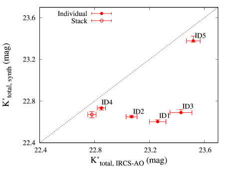
Figure 4: Synthetic $K^{\prime}$-band magnitude ($K^{\prime}_{total,synth}$) plotted against IRCS $K^{\prime}$-band magnitude ($K^{\prime}_{total,IRCS-AO}$) of our targets. The red filled circles show the individual objects. The red open circle shows the stack of ID$1$ to ID$4$.

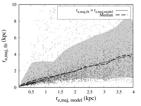
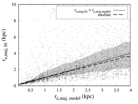
Figure 5: Top: Sizes measured by GALFIT ($r_{e,maj,fit}$) as a function of input size ($r_{e,maj,model}$) in our simulation for ID1. The solid line shows $r_{e,maj,model}=r_{e,maj,fit}$. The dashed curve and gray shaded regions show the median and 1$\sigma$ range of the $r_{e,maj,fit}$ at the given $r_{e,maj,model}$. Bottom: Similar to the top panel but for the stacked galaxy.

Table 3: Properties of the observed objects

ID	$z_{\rm phot}$	$K_{tot}$	$K^{\prime}_{tot,synth}\tablenotemark{b}$	$K^{\prime}_{tot,observed}$	$r_{e,maj}$	$M_{\star}$
		(mag)	(mag)	(mag)	(kpc)	($10^{11}~{}M_{\odot}$)
1	4.07	$22.47\pm 0.05$	$22.60^{+0.05}_{-0.05}$	$23.26\pm 0.06$	$0.92\pm 0.31$	1.58
2	3.83	$22.54\pm 0.05$	$22.69^{+0.06}_{-0.05}$	$23.43\pm 0.08$	$0.22\pm 0.21$	1.09
3	3.70	$22.55\pm 0.05$	$22.65^{+0.05}_{-0.05}$	$23.07\pm 0.04$	$0.63\pm 0.18$	1.04
4	4.24	$22.61\pm 0.05$	$22.73^{+0.05}_{-0.05}$	$22.85\pm 0.03$	$0.50\pm 0.21$	1.83
5	4.09	$23.35\pm 0.09$	$23.38^{+0.10}_{-0.04}$	$23.52\pm 0.05$	$1.70\pm 0.71$	1.13
STACK	…	$22.54\pm 0.03$	$22.67^{+0.03}_{-0.03}$	$22.78\pm 0.03$	$0.52\pm 0.18$	1.38

Table 4: GALFIT fittings of ID5 with the IRCS-AO $K^{\prime}$ and WFC3 $H$-band images

Band	mag	$r_{e,maj}$	$n$
	(mag)	(kpc)
$K^{\prime}$	$23.52\pm 0.05$	$1.70\pm 0.71$	$0.79_{0.5}^{2.99}$
$H$	$24.84\pm 0.02$	$1.19\pm 0.03$	$0.73\pm 0.03$

4.2 GALFIT fitting

The sizes of our targets are measured by fitting Sérsic profiles (Sersic, 1968) to their $K^{\prime}$-band images using GALFIT (Peng et al., 2002, 2010). GALFIT fits two-dimensional analytical functions convolved with a PSF to an observed galaxy image. Here we use a scale of $6.951$ kpc/arcsec in physical at $z=4$ for all the targets. We use the nearest star in the field of view or a star taken before and after the science exposures as the PSF reference star. We at first fit the Sérsic models in ranges of effective radius $r_{e}=0.2-12$ kpc and Sérsic index $n=0.5-10$. The fits are performed using an image cutout of 3.0 arcsec on a side for each object. The background values are estimated in an annulus between $2.9$ to $3.0$ arcsec from each object before Sérsic model fittings. As an initial guess, we use total magnitudes measured by SExtractor (Bertin & Arnouts, 1996), $r_{e}=1$ kpc and $n=1.4$. The results are not sensitive to this initial guess. In order to compare our results with van der Wel et al. (2014), who measured galaxies sizes out to $z\sim 3$, we here use the effective radius along the semi-major axis ($r_{e,maj}$).

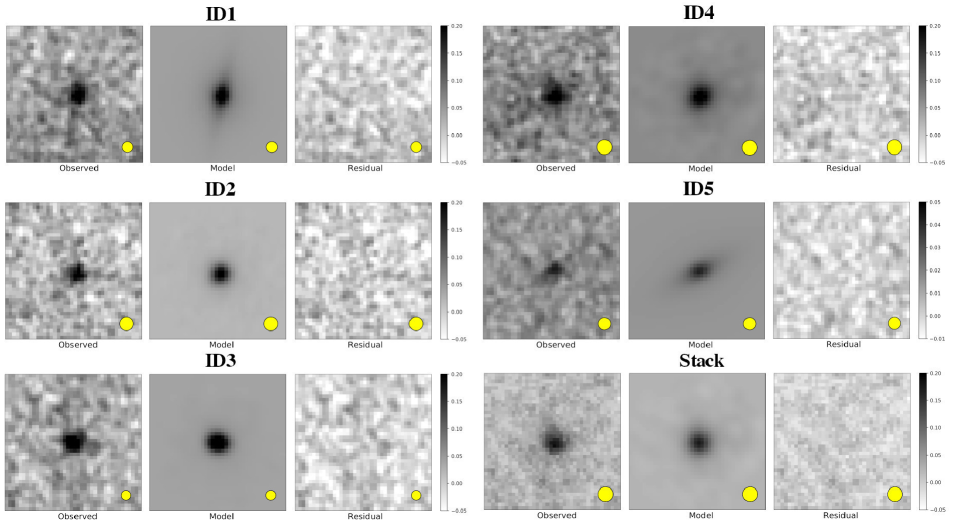
Figure 6: The observed images and GALFIT result for ID1 to ID5 and stacked galaxy. The observed images, best-fit Sérsic models, and residuals are shown from left to right. The sizes of the images are $2.1$ arcsec $\times$ $2.1$ arcsec. The yellow filled circles show the FWHM of the PSF size on each image.

4.3 GALFIT fitting errors

In Kubo et al. (2017), the morphologies of galaxies at $z\approx 3$ were studied by using the deeper $K^{\prime}$-band image taken with the same instrument with us and discussed the errors for GALFIT fittings on those images. We here discuss the possible errors in our size measurements following that work.

Let us start with the limitation by PSF. We are now studying the targets which can be hardly resolved even with our high resolution images. We should note that our results can be just an upper limit since the reduced $\chi^{2}$ values of Sérsic model fitting only marginally ($\Delta\chi^{2}\sim 0.01$) improves from that with PSF model fitting. In addition, the fits with models of different Sérsic indices $n=0.5\sim 5$ are equally good. Then we adopt the median of $r_{e,maj}$ of GALFIT fitting with $n=0.5,1,2,3,4~{}\&~{}5$ as the best-fit values.

In addition, there can be errors originated in a little PSF inconsistency. We ideally need to evaluate the PSF at the positions of the targets, but that is in practice difficult. We use a single PSF reference star either within the field of view or taken before/after the science exposures. Even though the target and PSF reference stars are taken in a same frame, as shown in Table 2, the distance between the tip-tilt star and the target, and that between the tip-tilt star and the PSF reference star are not the same. In case of our targets, we expect the PSF difference of $\lesssim 0.03$ arcsec according to the performance of AO188. However since the size of galaxies at $z\sim 4$ is very small, this may not be negligible. The separation between the PSF reference star and the tip-tilt star is always smaller than the separation between the target and the tip-tile star, i.e., the PSF we use in the fits is likely smaller than the real PSF at the object position. This leads us to over-estimate the size. Thus, our estimates are likely conservative. Kubo et al. (2017) reported that, this level of PSF inconsistency does not affect the measured sizes but on the other hand, it significantly affects the measured Sérsic indices, which we do not discuss in this paper.

Next, we test the accuracy of the GALFIT measurement by generating mock galaxy images following Kubo et al. (2017). We investigate the typical fitting errors by inserting artificial objects on the sky of the observed image, measuring the sizes of them and comparing the input and output structural parameters. We here use the coadd image of ID1 as the representative case of our sample. We generate artificial sources over a range of parameters; $K^{\prime}=22.6$ ($\approx K^{\prime}_{tot,synth}$ of ID1), $r_{e,maj}<4$ kpc, Sérsic indices $n=0-8$, and various axis ratios and position angles. They are convolved with the PSF reference star for ID1 and added to the sky of ID1 image. By repeating this simulation, we find that the median and standard deviation of the measured total magnitude are $23.0\pm 0.6$ in case $r_{e,maj,model}=0.5\sim 2$ kpc, which is consistent with the observed $K^{\prime}$-band total magnitude of ID1. In other words, the simulation reproduces the missing flux in the observation, suggesting that our simulation is reasonably realistic. We show the $r_{e,maj}$ of the mock galaxies ($r_{e,maj,model}$) v.s. those measured on them with GALFIT ($r_{e,maj,fit}$) in Fig. 5. Naively, we expect that small ($\lesssim 1$ kpc) objects are overestimated the sizes from the input sizes due to the limited resolution while large objects are underestimated since their outer profiles are buried in noise. We can see this tendency weakly. The standard deviation of Sérsic indices is $\sigma(n)=2.3$ (plot not shown). This again suggests that the Sérsic indices are hardly constrained with our data. Though we input various axis ratios, the measured axis ratios tend to be lower than 0.4, more asymmetric models are favored as the best-fit models. This may be caused by asymmetric distribution of noisy pixels around the source, since this tendency is soften at the depth of the stacked image. The best-fit models of ID1 and ID5 in Fig. 6 look elongated however it is not clear they are real signatures.

Finally, we compare the $r_{e,maj}$ measured with HST/WFC3 $H$-band image and our $K^{\prime}$-band images. Among our sample, only ID5 is within the Cosmic Assembly Near-IR Deep Extragalactic Legacy Survey (CANDELS; Grogin et al. 2011; Koekemoer et al. 2011). We summarize the comparison in Table. 4. They should not necessarily be the same as our result due to the wavelength difference but are a good comparison. The size estimates on these images are broadly consistent with each other, but our size estimate is slightly larger as expected from the simulation above. This may also imply that they show no strong rest-frame UV to optical color gradient due to age and/or metallicity gradient of the stellar population as well as attenuation by dust. The stellar population of these galaxies may be relatively simple. On the other hand, uncertainty in Sérsic indices is large for $K^{\prime}$, which is again consistent with the above indications.

Taken all the tests together, there is a small bias in our size measurements for individual objects in the sense that we tend to over-estimate the sizes by $\sim 30$ %. We do not account for this bias just to be conservative. Our estimates can thus be considered as reasonable upper limits.

4.4 Stacking analysis

We stack our targets to gain S/N and measure their average size. We exclude ID5 from the stacking because it is relatively fainter than the others. We smoothed the single exposure images of ID1 to ID4 to a common seeing of $0.23$ arcsec (that of ID4) by convolving with a Gaussian and then performed median stacking of them. The total $K^{\prime}$-band magnitude measured on the stacked image shows only a small amount of missing flux (10%, Fig. 4).

We repeat the same GALFIT simulation using the stacked image and PSF reference star for ID4 (Fig. 5, bottom). Similar to the individual galaxies, the reduced $\chi^{2}$ values of Sérsic model fitting only marginally improves from that with the PSF model fitting. The $r_{e,maj}$ errors are reduced greatly from the simulation for ID1. The bias in the size measurement marginally changes depending on the PSF adopted. This gives us a confidence on the measured sizes of QGs on our stacked image.

5 Results

The results of GALFIT fitting are shown in Fig. 6 and summarized in Table 3. The $r_{e,maj}$ of our targets range from $0.2-1.7$ kpc with the median and standard deviation being 0.6 kpc and 0.6 kpc, respectively. Our results indicate that massive QGs at $z\sim 4$ are indeed compact. As discussed above, the individual size estimates may suffer from the flux incompleteness (we are missing diffuse light), but we obtain a consistent result for the stacked galaxy; the $r_{e,maj}$ measured on the stack is $0.52\pm 0.18$ kpc, providing further support for the compact sizes. We also note that the possible systematic errors from the PSF inconsistency are not included in our size estimate errors, however, as we mentioned above, it may not affect them significantly.

Figure 7 shows the stellar mass v.s. $r_{e,maj}$ diagram of the QGs at $z\sim 4$. For comparison, we plot the size-stellar mass relation of QGs at $z=2.75$ measured at rest-frame optical (van der Wel et al., 2014) and at $z\sim 3.7$ measured at rest-frame UV (Straatman et al. (2015) using the catalog in Straatman et al. (2014) described above). Both studies select QGs with the photometric redshifts and $UVJ$ colors, and measure the size on HST/WFC3 $H$-band images from CANDELS. The QGs at $z\sim 4$ are below the size-stellar mass relation of QGs at $z=2.75$, suggesting that they have the physical sizes smaller than lower redshift ones. The size measured on the stack shown with the open square confirms this trend. The QGs at $z\sim 3.7$ have a somewhat large dispersion in size, but our targets have consistent sizes with some of their smallest objects. There are a few objects with a large size of $r_{e,maj}\sim 4$ kpc among QGs at $z\sim 3.7$ which are more consistent with the typical sizes of SFGs at $z=2.75$ (van der Wel et al., 2014). This might indicate the contamination of SFGs in their $UVJ$-selected QGs.

In Fig. 8, we show the rest-frame optical size-redshift relation of galaxies with $10^{11}~{}M_{\odot}\leq M_{\star}\leq 10^{11.5}~{}M_{\odot}$. The $r_{e,maj}$ at $z=0$, $0.75\leq z\leq 2.75$ and $z\sim 3.7$ are the median sizes of QGs with $10^{11}~{}M_{\odot}\leq M_{\star}\leq 10^{11.5}~{}M_{\odot}$ from Guo et al. (2009), van der Wel et al. (2014) and Straatman et al. (2015), respectively. The $z=3.1$ point is from Kubo et al. (2017) who measured the size of a QG with $M_{\star}\approx 2\times 10^{11}~{}M_{\odot}$ in a protocluster at the $K^{\prime}$-band using IRCS/AO188. Our stacked galaxy is shown as the open square. We extend the size-redshift relation of QGs out to $z\sim 4$ for the first time. The figure shows that the sizes of massive QGs continuously decreases with redshift up to $z=4$, an order of magnitude size evolution between $z=4$ and 0. This is a surprisingly strong evolution. Note that the size-stellar mass relation in van der Wel et al. (2014) show an upturn at $z=2.75$. This could be caused by the contamination of SFGs. In their $UVJ$ color diagram, the dispersions of color sequences of QGs and SFGs increase with redshift due to the observational errors and maybe the change of the SEDs of galaxies. Then it is expected that contaminants in galaxies selected as QGs increase with redshift. Straatman et al. (2015) also uses rest-frame $UVJ$ color selection but since they did not use the sample near the border of selection criterion, such contaminants may be reduced in their sample.

The size-redshift relation is often parameterized in a form $r_{e}/{\rm kpc}=A(1+z)^{\beta}$. van der Wel et al. (2014) find $A=11.2_{-2.1}^{+2.6}$ and $\beta=-1.32\pm 0.21$ for QGs with $10^{11}~{}M_{\odot}\leq M_{\star}\leq 10^{11.5}~{}M_{\odot}$ (dashed line in Fig. 8). Adding the results at $z>3$ and fitting at $0.75\leq z\leq 4$, we find $A=18.8\pm 3.0$ and $\beta=-1.9\pm 0.2$ (solid line), though it is hard to fit the whole redshift range with this form. Our results support a stronger size evolution of QGs compared to SFGs with $\beta\sim-1$ (e.g., van der Wel et al. 2014; Shibuya et al. 2015; Straatman et al. 2015) up to $z=4$.

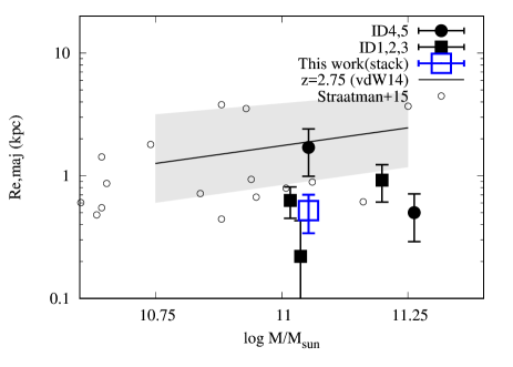
Figure 7: Stellar mass v.s. $r_{e,maj}$. The filled squares, filled circles and blue open square shows ID1-3, ID4-5 and the stack of ID 1-4, respectively. The solid line and the shaded area show the size-stellar mass relation for QGs at $z=2.75$ in van der Wel et al. (2014). The open circles show QGs at $z\sim 3.7$ measured the sizes at rest-frame UV in Straatman et al. (2015).

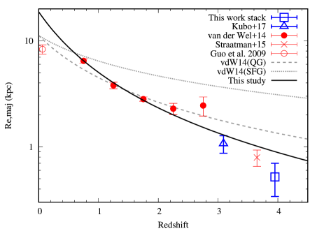
Figure 8: Size evolution of QGs with the stellar mass $10^{11}~{}M_{\odot}\leq M_{\star}\leq 10^{11.5}~{}M_{\odot}$ at up to $z=4$. The blue open square shows the stack of QGs at $z\sim 4$ in this study. The red open circle, filled circles and cross show the median $r_{e,maj}$ of QGs at $z=0$ from Guo et al. (2009), at $0.75\leq z\leq 2.75$ from van der Wel et al. (2014) and $z\sim 3.7$ from Straatman et al. (2015), respectively. The error bar of Guo et al. (2009) shows the $\sim 0.1$ dex difference between Shen et al. (2003) and Guo et al. (2009). The blue open triangle shows the QG with $M_{\star}\approx 2\times 10^{11}~{}M_{\odot}$ at $z=3.1$ in Kubo et al. (2017). The black solid curve shows $r_{e,maj}=A(1+z)^{\beta}$ fit in this study. The gray dashed and dotted lines show those for QGs and SFGs in van der Wel et al. (2014), respectively.

6 Discussion

In this study, we measure the size of massive QGs at $z\sim 4$ in the rest-frame optical wavelength for the first time based on the AO-assisted imaging using a ground-based telescope. There are a few possible uncertainties in our results.

One is contamination of AGNs which could make galaxies look compact. However, as shown in Fig. 2, the overall SEDs of our targets are dominated by evolved stellar populations as indicated by the strong Balmer break, which suggests that the continuum is dominated by stars. Thus, the AGN contamination, if any, is unlikely to significantly alter our results. Our targets are not detected in X-ray (Ueda et al., 2008) or MIR (Dunlop et al., 2007). Although only very active AGNs are detectable at the depth of the data at $z\sim 4$, this adds further support for no significant AGN contamination.

There is another question of the quiescence of our targets. Although the SED fits indicate that these galaxies are not actively forming stars, their quiescence should be further confirmed by other means. Gobat et al. (2017) detected significant far-IR fluxes from $BzK$ and $UVJ$-selected QGs, suggesting that the optical-nearIR selection does not always give a clean sample of QGs. Multi-wavelength follow-up observations of our targets are essential to fully confirm their quiescence. Efforts in this direction are underway.

Although we should further address these possible uncertainties in the future, it is interesting to discuss the origin and evolution of these extremely compact massive QGs at $z\sim 4$. In this section, we first discuss the extremely high stellar mass surface density of them and then focus on their size evolution on the evolving stellar mass track.

6.1 Extremely high stellar mass surface density

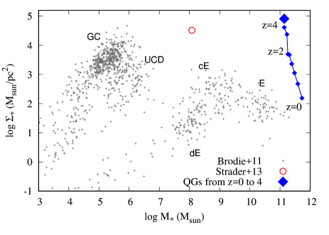
Figure 9: Surface stellar mass densities within effective radii v.s. stellar mass. The large blue diamond shows massive QGs at $z=4$. We also show its evolution track found in §6.2. The crosses show dispersion-supported systems in local Universe from Brodie et al. (2011) (GC=globular cluster; cE=compact elliptical; E=early-type galaxy; dE=dwarf elliptical). The red open circle shows the densest UCD reported in Strader et al. (2013).

It has been know that massive QGs at high redshift have extremely high stellar mass surface densities (e.g., van Dokkum et al. 2008). We compare the mean stellar mass surface densities within the effective radii of massive QGs at $z=4$ and dispersion-supported stellar systems in the local Universe (Brodie et al., 2011) in Fig. 9. Brodie et al. (2011) is originally given in $V$-band luminosity. We convert the $V$-band luminosity into stellar mass adopting $M_{\star}/L_{V}=3$ which is in case of a simple stellar population model with the age of $\sim 10$ Gyr adopting Chabrier (2003) IMF. Note that $M_{\star}/L_{V}$ can depend on the object type. We also show the densest ultra compact dwarf (UCD) reported in Strader et al. (2013) using its stellar mass from Seth et al. (2014).

It is interesting that high-z QGs and Globular clusters (GCs), consisting of the oldest stars of the Milky Way and thought to form at high redshifts, both have extremely high stellar mass surface densities, even though their typical mass differ by several orders of magnitude. Johnson et al. (2017) and Vanzella et al. (2017) find very low mass ($M_{\star}=$ a few $10^{6}~{}M_{\odot}$) extremely dense galaxies at $z=2-6$ with strong lensing. Though they are more massive than GCs, they imply that such ultra dense objects are commonly formed at high redshift. Given the high density and high gas fraction in the early Universe, we naturally expect that gas rich major mergers are one of the channels to form such extremely compact objects. In addition, cosmological numerical simulations predict that high-z galaxies are fed by streams of smooth gas and merging clumps from the cosmic web, and then they are settled into violent disc instabilities and end up with dense objects from dissipative compaction of gas and subsequent starburst (Dekel & Burkert, 2014; Zolotov et al., 2015).

We remark that at $z>4$, dusty SFGs (DSFGs) display very compact far-IR emitting regions that locate the ongoing starburst and establish a good proxy for the subsequent stellar remnant (e.g., Ikarashi et al. 2015; Oteo et al. 2017; Gómez-Guijarro et al. 2018). In a sample of six DSFGs at $z\sim 4.5$ with evidence of minor mergers, Gómez-Guijarro et al. (2018) measured a median stellar mass of $\log(M_{\star}/M_{\odot})=10.49\pm 0.32$ and far-IR sizes of $r_{e}=0.70\pm 0.29$ kpc. They expect the starburst to be completed in $\sim 50$ Myr, faster than the anticipated timescale for the observed mergers of $\sim 500$ Myr. Massive QGs at $z\sim 4$ studied here may have stopped star formation earlier ($z>5$) than these DSFGs, however, they present the capability of quickly building up and quenching of massive stellar cores at such high redshift. Further detailed studies of DSFGs with ALMA are awaited.

We finally quote Hopkins et al. (2010) which reports that the maximum stellar surface densities of GCs and high-z compact QGs are at the global stellar mass surface density limit regardless of their masses and propose that it is limited by feedback from young massive stars when star formation reaches the Eddington limit. Their results also imply that the densest objects are formed in the extreme situation which may be only achievable in the early Universe.

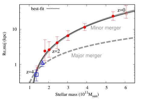
Figure 10: Size-stellar mass growth from massive QGs at $z=4$ taking the stellar mass evolution into account based on Marchesini et al. (2014). The $r_{e,maj}$ at each point are that extrapolated from van der Wel et al. (2014) (red filled circles), median and the 25-75% interval of the $r_{e,maj}$ of galaxies with $M_{\star}=10^{11.8}~{}M_{\odot}$ at $z=0$ from Guo et al. (2009) (red open circle), and observed values (others). The black dotted curve shows the best-fit curve. The gray solid and dashed curves show the toy models of size-stellar mass growth in cases of minor mergers ($r_{e,maj}\propto M_{\star}^{2}$) and major mergers ($r_{e,maj}\propto M_{\star}$), respectively.

6.2 Size evolution on the evolving stellar mass track

The size-redshift relation of massive QGs in Fig. 8 is measured at a fixed stellar mass. Galaxies grow with time and evolving cumulative number density determined in the semi-empirical approach using abundance matching has been used to find the progenitors of particular descendants (e.g., Behroozi et al. 2013). Marchesini et al. (2014) tracks the progenitors of ultra-massive galaxies today ($M_{\star}\approx 10^{11.8}~{}M_{\odot}$) by this method and find their stellar mass evolution as a function of redshift, $\log(M_{\star}/M_{\odot})=A+Bz+Cz^{2}$ where $A=11.801\pm 0.038$, $B=-0.304\pm 0.054$ and $C=0.039\pm 0.014$. This relation is based on the observations at $z<3$ but if we extrapolate it to $z\sim 4$, we find that massive QGs at $z\sim 4$ in this study are on this evolutionary track, i.e., they plausibly evolve into ultra-massive galaxies today.

Taking the stellar mass evolution into account using the stellar mass-redshift relation in Marchesini et al. (2014), we show the size-stellar mass evolution from massive QGs at $z=4$ in Fig. 10. The $r_{e,maj}$ are median and the 25-75% interval of the $r_{e,maj}$ of galaxies with $M_{\star}=10^{11.8}~{}M_{\odot}$ from Guo et al. (2009) at $z=0$, and extrapolated from the size-stellar mass relation at each redshift in van der Wel et al. (2014) at $0.25\leq z\leq 2.75$. The $r_{e,maj}$ at $z>3$ are the observed values since their stellar masses are on the stellar mass-redshift relation of Marchesini et al. (2014). The point at $z=3.1$ (Kubo et al., 2017) is not included in the fit, this is shown just for a reference. The top and bottom panels of Fig. 11 show the size evolution as functions of redshift and cosmic time, respectively. The size-redshift relation is fitted in a form of $r_{e,maj}/{\rm kpc}=A\times(1+z)^{B}$ where $A=44.1\pm 6.1$ and $B=-2.6\pm 0.2$ or $r_{e,maj}/{\rm kpc}=A\times B^{-(1+z)}$ where $A=69.7\pm 7.7$ and $B=2.7\pm 0.1$. If we fit the size-time relation in a form of $\log(r_{e,maj}/{\rm kpc})=A+B\log(t/\rm Gyr)$, we obtain $A=-0.56\pm 0.07$ and $B=1.91\pm 0.09$. We find that they grow in size by a factor $\sim 10$ in the first few Gyr and finally acquire the size $\sim 30$ times larger than that of a massive QG at $z=4$ by $z=0$. They have also evolved significantly in the stellar mass surface density (Fig. 9).

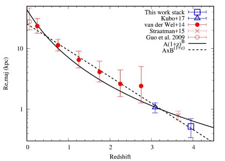
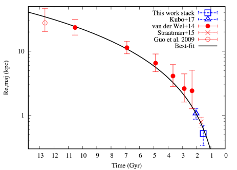
Figure 11: Top: Size-redshift relation of massive QGs taking the stellar mass evolution into account. The data points are the same as those in Fig. 10. The black solid curve and dashed line show the best-fit curves in forms of $r_{e,maj}/{\rm kpc}=A\times(1+z)^{B}$ and $r_{e,maj}/{\rm kpc}=A\times B^{-(1+z)}$, respectively. Bottom: Similar to the top panel but scaled in cosmic time and the black solid curve shows the best-fit curve in a form of $\log(r_{e,maj}/{\rm kpc})=A+B\log(t/\rm Gyr)$.

In order to constrain physical processes driving this rapid evolution, we compare the size-stellar mass growth to the two toy models shown in Fig. 10. We show size-stellar mass growth models via minor mergers (gray solid curve) and major mergers (gray dashed curve), which follow $r\propto M^{2}$ and $r\propto M$, respectively (Bezanson et al., 2009; Naab et al., 2009). The observed size-stellar mass growth closely follows that of minor mergers: it is fitted in a form $r_{e,maj}/{\rm kpc}=A\times(M_{\star}/10^{11}~{}M_{\odot})^{B}+C$ where $A=1.0\pm 0.4$, $B=1.9\pm 0.2$ and $C=-1.3\pm 0.6$ (black dotted curve). Similarly, van Dokkum et al. (2010) evaluates the size-stellar mass evolution of massive galaxies with $M_{\star}\approx 10^{11.45}~{}M_{\odot}$ at $z=0$ taking the stellar mass evolution into account by constant number density method. Although the samples and methods are different, they report $r_{e}\propto M^{2.08}$ evolution, similar to our result. Our result also agree with the prediction of the stellar mass and size growth of massive-end QGs with $M_{\star}\approx 10^{11.8}~{}M_{\odot}$ in Genel et al. (2018) based on the IllustrisTNG simulation. Taking all these results together, we conclude that the evolution of massive-end galaxies from $z=4$ is likely to be driven by minor mergers.

Note that lower mass galaxies may not necessarily follow the size growth found in this study. The mass dependent evolution has been predicted in cosmological numerical simulations. E.g., more moderate size growth of lower mass galaxies is predicted in Genel et al. (2018). The continual addition of massive galaxies to the quiescent population, so called progenitor bias may also contribute to the observed size growth (e.g., Carollo et al. 2013; Poggianti et al. 2013) though it alone may not be sufficient (Belli et al., 2015). Several studies reported that the observed merger rate is not capable for the size growth of high-z compact ellipticals (Williams et al., 2011; Newman et al., 2012; Man et al., 2016) but on the other hand, in situ star formation in satellites before mergers can push up the size-growth amount via minor mergers (Morishita & Ichikawa, 2016). It can also happen that the environment of the most massive galaxies is special. Massive compact elliptical at $z=3.09$ cited from Kubo et al. (2017) is in a dense group of massive galaxies capable for the ten times size growth at least. Further studies of not only compact massive quiescent galaxies themselves but also their environment are needed to understand what physical processes govern the size-stellar mass growth.

7 Conclusion

We have measured the rest-frame optical sizes of massive galaxies with suppressed star formation at $z\sim 4$ with IRCS and AO188 on the Subaru telescope. Although our measurements on individual galaxies are noisy, the more robust size measurements on the stacked object reveals that they have smaller physical sizes compared to lower redshift ones. This is the first measurement of the rest-frame optical sizes of QGs at $z\sim 4$. Their mean stellar mass surface density is similar to those of GCs, the densest objects of the Universe, although their masses differ by several orders of magnitude. This implies that the origin of the densest galaxies are due to the high density and high gas fraction in the early Universe. If we take the stellar mass evolution into account, they plausibly evolve into the most massive galaxies today and their stellar mass-size evolution is consistent with a scenario in which minor dry mergers drive the size growth.

We have shown that massive QGs at $z\sim 4$ are compact, but we have pushed the ability of current facilities close to the limit. Deeper and higher resolution imaging at $>2~{}\mu$m with AO on ground based large(r) telescopes and James Webb Space Telescope (JWST) are needed to make a leap from here.

References

- Barro et al. (2014) Barro, G., Faber, S. M., Pérez-González, P. G., et al. 2014, ApJ, 791, 52
- Barro et al. (2016) Barro, G., Kriek, M., Pérez-González, P. G., et al. 2016, ApJ, 827, L32
- Barro et al. (2017) Barro, G., Faber, S. M., Koo, D. C., et al. 2017, ApJ, 840, 47
- Behroozi et al. (2013) Behroozi, P. S., Marchesini, D., Wechsler, R. H., et al. 2013, ApJ, 777, L10
- Belli et al. (2015) Belli, S., Newman, A. B., & Ellis, R. S. 2015, ApJ, 799, 206
- Bertin & Arnouts (1996) Bertin, E., & Arnouts, S. 1996, A&AS, 117, 393
- Bezanson et al. (2009) Bezanson, R., van Dokkum, P. G., Tal, T., et al. 2009, ApJ, 697, 1290
- Bradshaw et al. (2013) Bradshaw, E. J., Almaini, O., Hartley, W. G., et al. 2013, MNRAS, 433, 194
- Brodie et al. (2011) Brodie, J. P., Romanowsky, A. J., Strader, J., & Forbes, D. A. 2011, AJ, 142, 199
- Bruzual & Charlot (2003) Bruzual, G., & Charlot, S. 2003, MNRAS, 344, 1000
- Calzetti et al. (1994) Calzetti, D., Kinney, A. L., & Storchi-Bergmann, T. 1994, ApJ, 429, 582
- Carollo et al. (2013) Carollo, C. M., Bschorr, T. J., Renzini, A., et al. 2013, ApJ, 773, 112
- Chabrier (2003) Chabrier, G. 2003, PASP, 115, 763
- Daddi et al. (2005) Daddi, E., Renzini, A., Pirzkal, N., et al. 2005, ApJ, 626, 680
- Dekel & Burkert (2014) Dekel, A., & Burkert, A. 2014, MNRAS, 438, 1870
- Dekel et al. (2009) Dekel, A., Sari, R., & Ceverino, D. 2009, ApJ, 703, 785
- Dunlop et al. (2007) Dunlop, J., Akiyama, M., Alexander, D., et al. 2007, Spitzer Proposal,
- Elmegreen et al. (2008) Elmegreen, B. G., Bournaud, F., & Elmegreen, D. M. 2008, ApJ, 688, 67-77
- Fan et al. (2008) Fan, L., Lapi, A., De Zotti, G., & Danese, L. 2008, ApJ, 689, L101
- Furusawa et al. (2008) Furusawa, H., Kosugi, G., Akiyama, M., et al. 2008, ApJS, 176, 1-18
- Genel et al. (2018) Genel, S., Nelson, D., Pillepich, A., et al. 2018, MNRAS, 474, 3976
- Glazebrook et al. (2017) Glazebrook, K., Schreiber, C., Labbé, I., et al. 2017, Nature, 544, 71
- Gobat et al. (2017) Gobat, R., Daddi, E., Magdis, G., et al. 2017, arXiv:1703.02207
- Gómez-Guijarro et al. (2018) Gómez-Guijarro, C., Toft, S., Karim, A., et al. 2018, ApJ, 856, 121
- Grogin et al. (2011) Grogin, N. A., Kocevski, D. D., Faber, S. M., et al. 2011, ApJS, 197, 35
- Guo et al. (2009) Guo, Y., McIntosh, D. H., Mo, H. J., et al. 2009, MNRAS, 398, 1129
- Hayano et al. (2008) Hayano, Y., Takami, H., Guyon, O., et al. 2008, Proc. SPIE, 7015, 701510
- Hayano et al. (2010) Hayano, Y., Takami, H., Oya, S., et al. 2010, Proc. SPIE, 7736, 77360N
- Hopkins et al. (2008) Hopkins, P. F., Hernquist, L., Cox, T. J., & Kereš, D. 2008, ApJS, 175, 356-389
- Hopkins et al. (2010) Hopkins, P. F., Murray, N., Quataert, E., & Thompson, T. A. 2010, MNRAS, 401, L19
- Ikarashi et al. (2015) Ikarashi, S., Ivison, R. J., Caputi, K. I., et al. 2015, ApJ, 810, 133
- Ikarashi et al. (2017) Ikarashi, S., Caputi, K. I., Ohta, K., et al. 2017, ApJ, 849, L36
- Inoue (2011) Inoue, A. K. 2011, MNRAS, 415, 2920
- Johnson et al. (2017) Johnson, T. L., Sharon, K., Gladders, M. D., et al. 2017, ApJ, 843, 78
- Kauffmann et al. (2003) Kauffmann, G., Heckman, T. M., Tremonti, C., et al. 2003, MNRAS, 346, 1055
- Kobayashi et al. (2000) Kobayashi, N., Tokunaga, A. T., Terada, H., et al. 2000, Proc. SPIE, 4008, 1056
- Koekemoer et al. (2011) Koekemoer, A. M., Faber, S. M., Ferguson, H. C., et al. 2011, ApJS, 197, 36
- Kubo et al. (2017) Kubo, M., Yamada, T., Ichikawa, T., et al. 2017, MNRAS, 469, 2235
- Labbé et al. (2005) Labbé, I., Huang, J., Franx, M., et al. 2005, ApJ, 624, L81
- Lawrence et al. (2007) Lawrence, A., Warren, S. J., Almaini, O., et al. 2007, MNRAS, 379, 1599
- Man et al. (2016) Man, A. W. S., Zirm, A. W., & Toft, S. 2016, ApJ, 830, 89
- Marchesini et al. (2014) Marchesini, D., Muzzin, A., Stefanon, M., et al. 2014, ApJ, 794, 65
- McLure et al. (2013) McLure, R. J., Pearce, H. J., Dunlop, J. S., et al. 2013, MNRAS, 428, 1088
- Merlin et al. (2015) Merlin, E., Fontana, A., Ferguson, H. C., et al. 2016, A&AS, 582, 15
- Morishita & Ichikawa (2016) Morishita, T., & Ichikawa, T. 2016, ApJ, 816, 87
- Naab et al. (2009) Naab, T., Johansson, P. H., & Ostriker, J. P. 2009, ApJ, 699, L178
- Newman et al. (2012) Newman, A. B., Ellis, R. S., Bundy, K., & Treu, T. 2012, ApJ, 746, 162
- Oteo et al. (2017) Oteo, I., Ivison, R. J., Negrello, M., et al. 2017, arXiv:1709.04191
- Peng et al. (2010) Peng, C. Y., Ho, L. C., Impey, C. D., & Rix, H.-W. 2010, AJ, 139, 2097
- Peng et al. (2002) Peng, C. Y., Ho, L. C., Impey, C. D., & Rix, H.-W. 2002, AJ, 124, 266
- Pickles (1998) Pickles, A. J. 1998, PASP, 110, 863
- Poggianti et al. (2013) Poggianti, B. M., Moretti, A., Calvi, R., et al. 2013, ApJ, 777, 125
- Schreiber et al. (2018) Schreiber, C., Labbé, I., Glazebrook, K., et al. 2018, A&A, 611, A22
- Sersic (1968) Sersic, J. L. 1968, Cordoba, Argentina: Observatorio Astronomico, 1968,
- Seth et al. (2014) Seth, A. C., van den Bosch, R., Mieske, S., et al. 2014, Nature, 513, 398
- Shen et al. (2003) Shen, S., Mo, H. J., White, S. D. M., et al. 2003, MNRAS, 343, 978
- Shibuya et al. (2015) Shibuya, T., Ouchi, M., & Harikane, Y. 2015, ApJS, 219, 15
- Shibuya et al. (2016) Shibuya, T., Ouchi, M., Kubo, M., & Harikane, Y. 2016, ApJ, 821, 72
- Simpson et al. (2017) Simpson, J. M., Smail, I., Wang, W.-H., et al. 2017, ApJ, 844, L10
- Strader et al. (2013) Strader, J., Seth, A. C., Forbes, D. A., et al. 2013, ApJ, 775, L6
- Straatman et al. (2014) Straatman, C. M. S., Labbé, I., Spitler, L. R., et al. 2014, ApJ, 783, L14
- Straatman et al. (2015) Straatman, C. M. S., Labbé, I., Spitler, L. R., et al. 2015, ApJ, 808, L29
- Straatman et al. (2016) Straatman, C. M. S., Spitler, L. R., Quadri, R. F., et al. 2016, ApJ, 830, 51
- Tadaki et al. (2015) Tadaki, K.-i., Kohno, K., Kodama, T., et al. 2015, ApJ, 811, L3
- Tanaka (2015) Tanaka, M. 2015, ApJ, 801, 20
- Tanaka et al. (2017) Tanaka, M., Coupon, J., Hsieh, B.-C., et al. 2017, arXiv:1704.05988
- Toft et al. (2007) Toft, S., van Dokkum, P., Franx, M., et al. 2007, ApJ, 671, 285
- Toft et al. (2009) Toft, S., Franx, M., van Dokkum, P., et al. 2009, ApJ, 705, 255
- Toft et al. (2014) Toft, S., Smolčić, V., Magnelli, B., et al. 2014, ApJ, 782, 68
- Tokunaga et al. (1998) Tokunaga, A. T., Kobayashi, N., Bell, J., et al. 1998, Proc. SPIE, 3354, 512
- Trujillo et al. (2006) Trujillo, I., Feulner, G., Goranova, Y., et al. 2006, MNRAS, 373, L36
- Ueda et al. (2008) Ueda, Y., Watson, M. G., Stewart, I. M., et al. 2008, ApJS, 179, 124-141
- Vanzella et al. (2017) Vanzella, E., Calura, F., Meneghetti, M., et al. 2017, MNRAS, 467, 4304
- van der Wel et al. (2014) van der Wel, A., Franx, M., van Dokkum, P. G., et al. 2014, ApJ, 788, 28
- van Dokkum et al. (2008) van Dokkum, P. G., Franx, M., Kriek, M., et al. 2008, ApJ, 677, L5
- van Dokkum et al. (2010) van Dokkum, P. G., Whitaker, K. E., Brammer, G., et al. 2010, ApJ, 709, 1018
- van Dokkum et al. (2014) van Dokkum, P. G., Bezanson, R., van der Wel, A., et al. 2014, ApJ, 791, 45
- Wellons et al. (2015) Wellons, S., Torrey, P., Ma, C.-P., et al. 2015, MNRAS, 449, 361
- Williams et al. (2009) Williams, R. J., Quadri, R. F., Franx, M., van Dokkum, P., & Labbé, I. 2009, ApJ, 691, 1879
- Williams et al. (2011) Williams, R. J., Quadri, R. F., & Franx, M. 2011, ApJ, 738, L25
- Zolotov et al. (2015) Zolotov, A., Dekel, A., Mandelker, N., et al. 2015, MNRAS, 450, 2327