nIFTy galaxy cluster simulations VI: the dynamical imprint of substructure on gaseous cluster outskirts.

Abstract

Galaxy cluster outskirts mark the transition region from the mildly non-linear cosmic web to the highly non-linear, virialised, cluster interior. It is in this transition region that the intra-cluster medium (ICM) begins to influence the properties of accreting galaxies and groups, as ram pressure impacts a galaxy’s cold gas content and subsequent star formation rate. Conversely, the thermodynamical properties of the ICM in this transition region should also feel the influence of accreting substructure (i.e. galaxies and groups), whose passage can drive shocks. In this paper, we use a suite of cosmological hydrodynamical zoom simulations of a single galaxy cluster, drawn from the nIFTy comparison project, to study how the dynamics of substructure accreted from the cosmic web influences the thermodynamical properties of the ICM in the cluster’s outskirts. We demonstrate how features evident in radial profiles of the ICM (e.g. gas density and temperature) can be linked to strong shocks, transient and short-lived in nature, driven by the passage of substructure. The range of astrophysical codes and galaxy formation models in our comparison are broadly consistent in their predictions (e.g. agreeing when and where shocks occur, but differing in how strong shocks will be); this is as we would expect of a process driven by large-scale gravitational dynamics and strong, inefficently radiating, shocks. This suggests that mapping such shock structures in the ICM in a cluster’s outskirts (via e.g. radio synchrotron emission) could provide a complementary measure of its recent merger and accretion history.

1 Introduction

Galaxy clusters are the most massive virialised objects in the Universe, and are widely used as a powerful testbed for our theories of dark matter, dark energy, and galaxy formation and evolution, as well as cosmological parameter estimation (e.g., Kravtsov & Borgani, 2012; Mantz et al., 2014, 2016; Sartoris et al., 2016). Furthermore, they are striking signposts of the cosmic web, anchoring the large-scale network of filaments, sheets, and voids (e.g., Vazza et al., 2011; Durret et al., 2016; Martizzi, et al., 2019).

The imprint of this cosmic web can be inferred from the spatial and kinematical distribution of cluster galaxies (e.g., Knebe et al., 2004; Bailin & Steinmetz, 2005; Pimbblet, 2005; Hao et al., 2011; Song & Lee, 2012; Tempel et al., 2015). However, its influence should also be evident in the presence of accretion-driven shocks in the intra-cluster medium (ICM), especially at large cluster-centric radius (e.g., Tozzi et al., 2000; Ryu et al., 2003; Vazza et al., 2011). Such shocks arise naturally from cosmological accretion of gas onto the cluster from the warm ($T\lesssim 10^{4}-10^{6}\,{\rm K}$) diffuse inter-galactic medium (IGM) that resides in its lower density environs (see, e.g., Davé et al. 2001, and more recently Cui, et al. 2018 and Martizzi, et al. 2019). This gas will be accelerated gravitationally to peculiar velocities of order $\sim\!1000\,{\rm km}\,{\rm s}^{-1}$ during infall, which will produce strong shocks (e.g., Zinger et al., 2018) that give rise to various forms of non-thermal emission, ranging from high energy X-rays and $\gamma$-rays (e.g., Keshet et al., 2003, 2004; Zandanel et al., 2014), to radio continuum emission in the form of synchrotron radiation as electrons spiral along magnetic fields (Hoeft et al., 2008; Vazza, Brunetti, & Gheller, 2009).

Both observations and simulations show trends between a cluster’s merging and mass accretion history - which, observationally, are inferred from estimates of its dynamical state - and properties of its ICM, such as gas ellipticity (e.g., Chen et al., 2019), turbulent motions (e.g., Nagai et al., 2013; Avestruz, Nagai & Lau, 2016; Lau et al., 2017; Shi, Nagai & Lau, 2018), and the presence of density and pressure inhomogeneities (e.g., Nagai & Lau, 2011; Zhuravleva et al., 2013; Roncarelli et al., 2013; Lau et al., 2015; Tchernin, et al., 2016). This is of particular interest because these trends contribute to biases in cluster mass estimates (e.g. Zhuravleva et al., 2013); for example, gas turbulence and accelerations undermine assumptions of hydro-static equilibrium, which can underestimate a cluster’s true mass by between $\sim 5$ and 20 per cent (e.g., Nelson et al., 2014), while inhomogeneities drive clumping factors that boost estimates of the X-ray emissivity (e.g. Planelles, et al., 2017; Ghirardini, et al., 2018), which can be up to 40 per cent in the cluster outskirts, leading to cluster masses being underestimated by up to $\sim 30$ per cent (e.g., Rasia et al., 2014).

However, examining how substructure impacts properties of the ICM is of more general, astrophysical, interest. Examining the nature and origin of these trends between a cluster’s assembly history, its dynamical state, and evidence of inhomogeneities in its ICM, can help to clarify our understanding of how different physical processes can shape the ICM. For example, what are the relative contributions to turbulence of, for example, AGN jets and outflows compared to infalling substructures, and how does this change with position within the cluster and its dynamical age? Developing understanding in this way can provide theoretical insights into potentially new and powerful observable signatures and tests of cluster assembly.

Previous theoretical studies have investigated how merging and accretion influence the thermodynamical structure of the ICM (e.g., Avestruz, Nagai & Lau, 2016) using a statistical approach to infer the likely contribution of substructure (such as, e.g., using the density distribution in radial bins to decompose the ICM into smooth and clumpy components; cf. Zhuravleva et al., 2013), and comparing to the degree to which a cluster is considered dynamically relaxed (e.g. Zhuravleva et al., 2013; Rasia et al., 2014; Ota, Nagai & Lau, 2018; Zinger et al., 2018) or by quantifying its assembly history by measuring mass growth over time (e.g. Nelson et al., 2014; Lau et al., 2015). In this study, we take a complementary approach; we look in detail at how the passage of substructures through the ICM, tracked from infall from the cosmic web, influence its thermodynamical properties, as inferred from radial profiles of density, temperature, and radial velocity. In particular, we focus our analysis on ICM properties in the cluster outskirts, between $0.3\,R_{200}$ and $\sim(2-3)\,R_{200}$. It is here that we expect the signature of mergers and accretion to be most pronounced (see, e.g., Lau et al., 2015) - we reason that infalling substructures are likely to drive shocks into their surroundings when they are at their most gas-rich, subsequent to their accretion onto the cluster from the cosmic web - and we expect the effects of feedback to be secondary.

We base our analysis on a suite of cosmological zoom simulations of a single massive galaxy cluster, run with a range of state-of-the-art astrophysical codes - spanning mesh- and particle-based hydrodynamics solvers, as well as galaxy formation prescriptions - as part of the nIFTy galaxy cluster comparison project (see Sembolini et al., 2016a, and subsequent papers). Previous papers in this series (e.g., Sembolini et al., 2016a; Cui et al., 2016; Sembolini et al., 2016b) have demonstrated that there are significant differences between code predictions in the inner parts of clusters, reflecting both the choice of hydrodynamics solver and the adopted prescription for galaxy formation. This allows us to assess if ICM properties in the outskirts are similarly affected. If shocks driven by infalling substructures are driving turbulence and inhomogeneities in density and pressure, then we might expect systematic differences in the strength and duration of shocks because of the choice of hydrodynamics solver - as has been suggested by the work of Rasia et al. (2014) - but broad agreement in the timing and locations of shocks because substructure orbits will be governed by the large-scale gravitational field.

The structure of this paper is as follows. In §2, we describe briefly the simulations we have used, including how they were set up and their bulk properties at $z$=0. In §3, we present our main results – connecting features evident in the radial profiles of ICM properties (gas density, temperature, and kinematics) with substructure in § 3.1; exploring how the dynamics of substructure is imprinted on the ICM in § 3.2; and demonstrating the influence of the cosmic web in § 3.3. Finally, we summarise our results in §4.

2 The Data

2.1 The simulations

Our analysis focuses on cosmological hydrodynamical zoom simulations of a single galaxy cluster – “Cluster 19” from the MUSIC suite (Sembolini et al., 2013; Biffi et al., 2014; Sembolini et al., 2014) and identified originally in the MultiDark $2048^{3}$ particle parent cosmological $N$-body simulation (Prada et al., 2012). The adopted cosmology assumes total matter, baryon, and dark energy density parameters $(\Omega_{\rm m},\Omega_{\rm b},\Omega_{\Lambda})$=(0.27,0.0469,0.73); a power spectrum normalisation of $\sigma_{8}$=0.82; a primordial spectral index of $n$=0.95; and a dimensionless Hubble parameter of $h$=0.7, all in accord with the WMAP7+BAO+SNI dataset of Komatsu et al. (2011).

Initial conditions for all of the MUSIC clusters were generated using the approach of Klypin et al. (2001), which can be summarised as follows;

1. All particles within a sphere of radius $6h^{-1}{\rm Mpc}$ at $z$=0 centred on the cluster in the parent MultiDark simulation are found in the low-resolution $256^{3}$ particle version of the parent.

2. These particles are mapped back to the parent’s initial conditions to identify the Lagrangian region from which they originated, from which a mask is created.

3. The initial conditions of the parent simulation are re-generated on a finer mesh of size $4096^{3}$, a factor of 8 increase in mass resolution relative to the parent simulation.

4. The mask is then applied to the $4096^{3}$ particle dataset, such that particles within the masked region are retained and those outside of the mask are binned to produce coarser mass resolution tidal particles, equivalent to the low-resolution $256^{3}$ version of the parent.

The result is a set of initial conditions in which particles in the high resolution patch have a mass resolution a factor of 8 higher than in the parent run, corresponding to dark matter and gas particle masses of m${}_{\rm DM}=9.01\times 10^{8}h^{-1}{\rm M}_{\odot}$ and m${}_{\rm gas}=1.9\times 10^{8}h^{-1}{\rm M}_{\odot}$ respectively.

We used a selection of astrophysical codes - Arepo, G2-X, G3-MUSIC, G3-OWLS, and G3-X - and their associated galaxy formation models (non-radiative and full physics) in this paper; in the cases of Arepo and G3-MUSIC, we included two variants of their galaxy formation models, with (Arepo-IL) and without AGN feedback - (Arepo-SH, G3-MUSIC-SH, and G3-MUSIC-PS). Key features are presented in the Appendix, and we refer the interested reader to Sembolini et al. (2016b) for more details. We use only codes that have used the same aligned parameters (see the Table 4 in Sembolini et al., 2016a) to re-simulate the selected cluster; these govern the accuracy of the gravity solvers, and by requiring alignment we ensure that cluster features that are driven by gravity - for example, large-scale filamentary structure, orientation, timing of merger and accretion events - should be consistent between runs. This allows us to focus differences between results that are driven by either the hydrodynamics solver or the adopted galaxy formation prescription.

2.2 Structure finding

We have used the phase-space structure-finder VELOCIraptor (Elahi et al., 2019) to identify the main cluster and its substructure. VELOCIraptor identifies particle groups using a 3 dimensional friends-of-friends (FOF) algorithm and then refines each 3D-FOF group using a FOF algorithm applied to the full 6 dimensional phase-space. This 6D-FOF group catalogue is cleaned to correct for sets of halos that are combined artificially into a more massive system, arising from spurious bridges of particles between halos that occur during the early stages of mergers; this is done using the velocity dispersions of the 3D-FOF groups. Each 6D-FOF halo is then decomposed into a smooth background and its substructures by applying the phase-space FOF algorithm recursively, locating sets of particles that are dynamically distinct from the background. This approach is capable of finding both subhaloes and streams associated with tidally disrupted systems (Elahi et al., 2013).

Table 1: Cluster Properties at $z$=0. Here we give (1) the virial mass, ${M}_{200}$, as defined in the text; (2) $R_{200}$, the corresponding virial radius; (3) $f_{\rm g}$, the fraction of ${\rm M}_{200}$ in gas; (4) the centre-of-mass offset $\Delta R=(\vec{R}_{\rm cen}-\vec{R}_{\rm cm})/R_{200}$; and (5,6) $\sigma_{\rm 3D}^{\rm d}$, and $\sigma_{\rm 3D}^{\rm g}$, the 3D velocity dispersions of all the dark matter and gas particles within ${\rm R}_{200}$.

$M_{200}$	$R_{200}$	$f_{\rm g}$	$\Delta R$	$\sigma_{\rm 3D}^{\rm d,g}$
[$h^{-1}{\rm M}_{\odot}$]	[$h^{-1}{\rm Mpc}$]			[km/s]
$1.107\times 10^{15}$	1.682	0.1629	0.04	1960 / 950

Cluster 19 has been studied extensively as part of the nIFTy galaxy cluster comparison project (cf. Sembolini et al., 2016a, and subsequent papers), and its $z$=0 properties in the fiducial G3-MUSIC Full Physics run are given in Table 1. We follow the standard convention of defining cluster mass as $M_{200}$, the mass enclosed within a spherical region of radius $R_{200}$ encompassing an overdensity of 200 times the critical density $\rho_{\rm crit}$ at the given redshift $z$, i.e.

$$M_{200}=\frac{4\pi}{3}200\rho_{\rm crit}R_{200}^{3}.$$ (1)

Following previous studies (e.g., Thomas et al., 1998; Power et al., 2012), we use the centre-of-mass offset to quantify the cluster’s dynamical state,

$$\Delta R=(\vec{R}_{\rm cen}-\vec{R}_{\rm cm})/R_{200},$$ (2)

where $\vec{R}_{\rm cm}$ is the centre of mass of material within $R_{200}$ and $\vec{R}_{\rm cen}$ corresponds approximately to the centre of the densest substructure within $R_{200}$ as calculated via the iterative method of Power et al. (2003). The measured value of $\Delta R$=0.04 indicates that the cluster is relatively dynamically relaxed, which is consistent with a visual impression of the cluster (see below).

2.3 Visual Impression

In Figure 1, we show projected gas density (upper panels) and temperature maps (lower panel) for the G3-MUSIC run at $z$=0. On the left, we show results for the fiducial non-radiative run, while on the right, we show one of its full physics counterparts. Positions are plotted relative to $\vec{R}_{\rm cen}$ and normalised by $R_{200}$, both evaluated for the particular run; we project from within a cube of side $7\,R_{200}$, or equivalently out to a radius of $3.25\,R_{200}$. The projected density maps were calcuated using the py-sphviewer package (Benitez-Llambay, 2015), which computes smoothing lengths on a per particle basis and so naturally adapts to regions of local density, allowing fine structure to be discerned. For projected temperature maps, we use matplotlib’s hexbin with a fine grid of $1536^{2}$.

Because the simulations were run with aligned parameters, we find excellent agreement between the runs on intermediate-to-large scales; the structure of the filamentary network, as traced by the gas, in which the cluster is embedded is in very good agreement, and there is excellent correspondence between the positions of the more massive substructures (cf. Sembolini et al., 2016a). The differences we see within the core of the cluster have been studied previously (cf. Cui et al., 2016), and are driven by hydrodynamical shocks and the physics of galaxy formation (i.e. cooling and feedback).

In contrast, we see clear differences between the runs on small-scales. In the projected gas density maps, we see more high-density small-scale structure in the full physics run than in the galaxy formation run throughout the volume, as we would expect in the presence of radiative cooling. However, in the projected temperature maps, we see more sharply defined features in the non-radiative run - for example, the ridge extending from upper-left to lower-right in the cluster core, as well as several cool, dense knots with $R_{200}$ - than in the full physics run. We shall return to these observations in the next section.

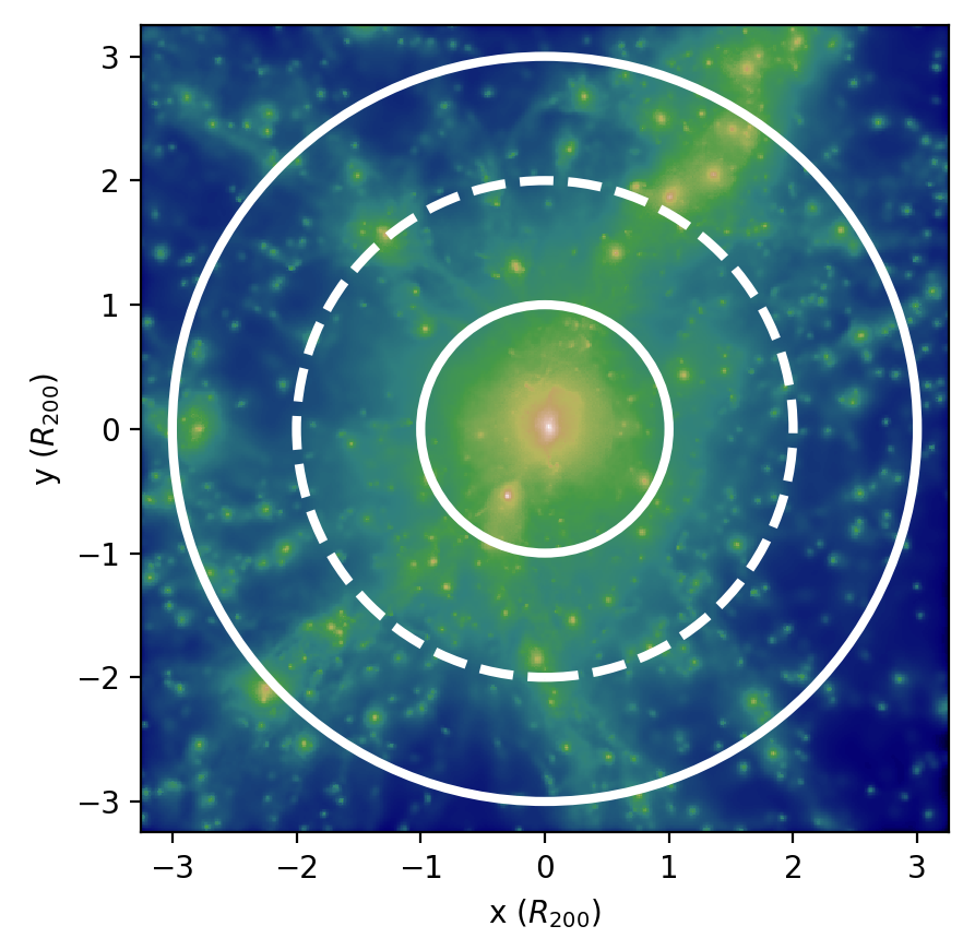
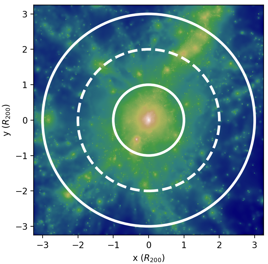
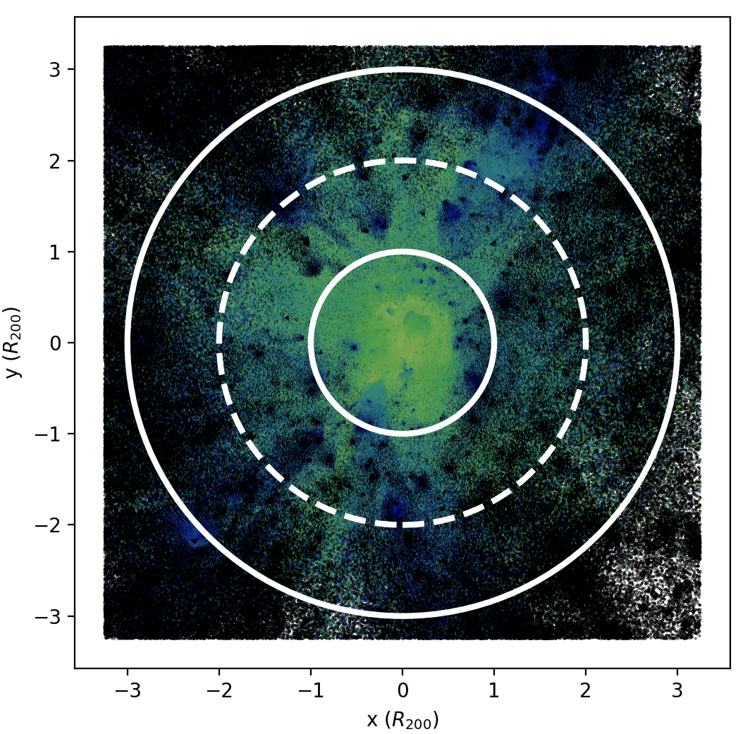
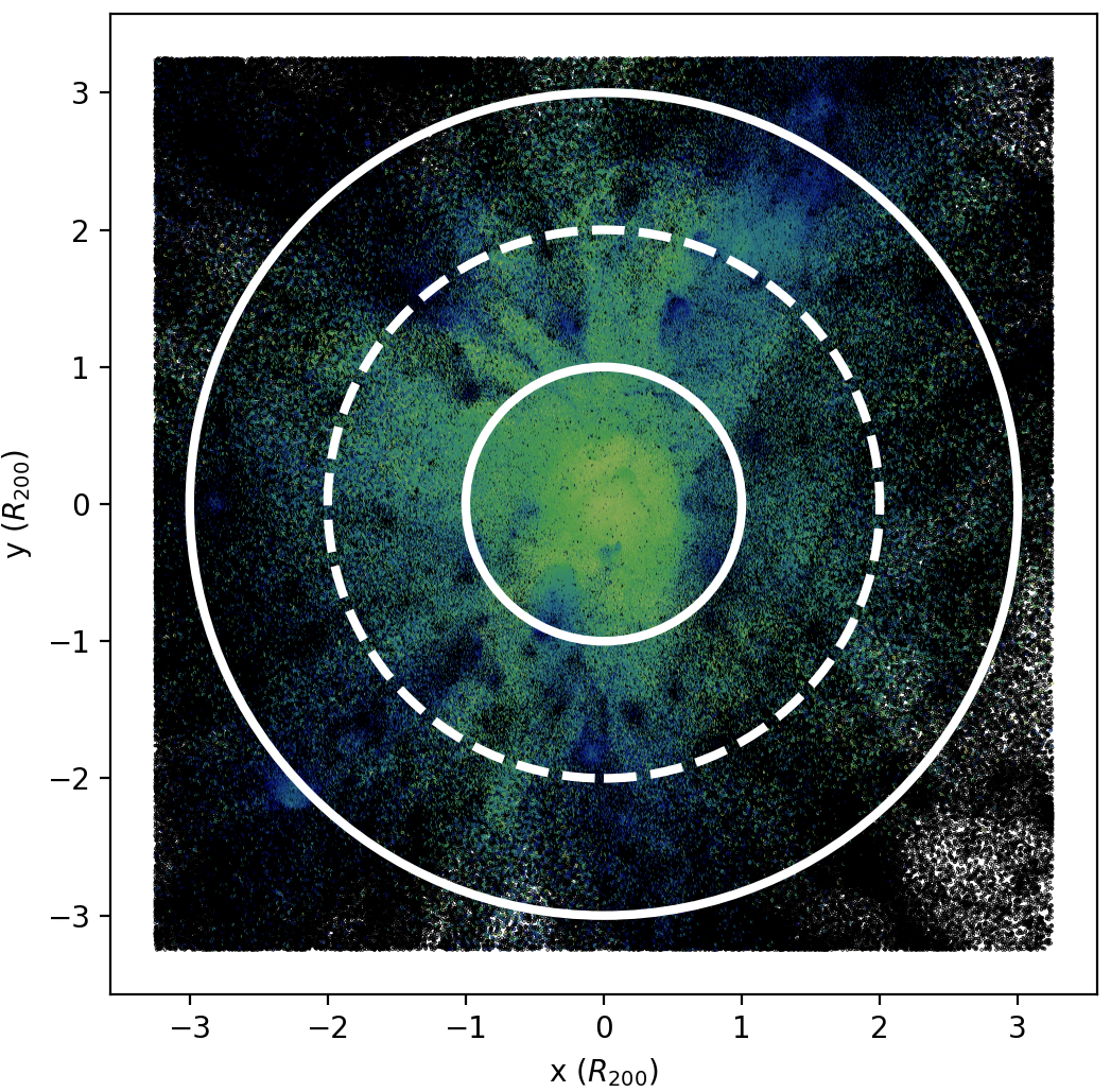
Figure 1: A visual impression of Cluster 19 and its local environment. Here we show projected gas densities (upper panels) and temperatures (lower panels) in the fiducial non-radiative and full physics G3-MUSIC runs at $z$=0. Inner solid/dashed/outer solid circles indicate 1/2/3 times $R_{200}$. In plotting maps of projected gas densities with py-sphviewer (Benitez-Llambay, 2015), smoothing lengths are estimated on a per particle basis before projection, allowing for fine detail in gas density to be discrened; temperature maps are constructed using the matplotlib hexbin function.

3 Results

We now investigate the thermodynamical properties of the ICM in the outskirts of the cluster at $z$=0. In particular, we focus on radial profiles of gas density, temperature, and radial velocity in the regime $0.3\leq R/R_{\rm 200}\lesssim 3$, and investigate in detail the relationship between structures evident in these profiles, which we interpret as arising from shocks, and the orbital motions of substructures (§ 3.2) and accretion from the cosmic web (§ 3.3). Because we have a range of astrophysical codes and galaxy formation prescriptions, we can estimate the degree of variation that arises. Our reference simulation is the non-radiative G3-MUSIC run, and residuals (when shown) are with respect to this run. All figures include data from both non-radiative and full physics simulations, unless otherwise stated.

3.1 Radial profiles of ICM gas properties

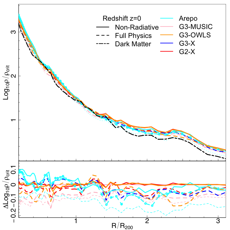
Figure 2: Spherically averaged gas density profiles at $z$=0. In the upper panel, we show the spherically averaged gas density profiles measured in the non-radiative runs (solid curves) and full physics runs (dashed curves). Here radii are normalised to the value of $R_{200}$ in the G3-MUSIC non-radiative run; densities are in units of $\rho_{\rm crit}$ at $z$=0, 2.7755$\times 10^{11}\,h^{2}\,{\rm M}_{\odot}\,{\rm Mpc}^{-3}$. For reference, we show the heavy dotted-dashed curve is the dark matter density profile (as found in the dark matter only G3-MUSIC reference run) scaled by the cosmic baryon density, $\Omega_{\rm bar}$/$\Omega_{\rm m}$. In the lower panel, we show the residuals of each of these profiles with respect to our G3-MUSIC non-radiative reference run. Note that there are two sets of Arepo and G3-MUSIC full physics runs - the Arepo-IL run with AGN (heavy dashed curves with filled circles), the Arepo-SH run with stellar feedback but without AGN (light dashed curves), and the G3-MUSIC-SH and G3-MUSIC-PS runs (heavy and light dashed curves) with stellar feedback and without AGN.

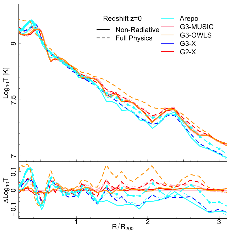
Figure 3: Spherically averaged gas temperature profiles at $z$=0. In the upper panel, we show the spherically averaged gas density profiles measured in the non-radiative runs (solid curves) and full physics runs (dashed curves). Radii are again normalised to $R_{200}$. In the lower panel, we show the residuals of each of these profiles with respect to the G3-MUSIC non-radiative run. We follow the same convention as in Figure 2 to distinguish between the different full physics Arepo and G3-MUSIC runs.

We begin our analysis by considering spherically averaged gas density and temperature profiles measured in the non-radiative (solid curves) and full physics (long dashed curves) simulations in our sample. Here we estimate the gas density at radius $R$ measured with respect to $\vec{R}_{\rm cen}$ as the total gas mass (i.e. summation over gas particle masses) within a spherical shell, divided by the volume of the shell; gas temperature is deduced from the average, mass-weighted, specific internal energy of particles in the shell, multiplied by $3\mu\,m_{p}/2\,k_{\rm B}$, where $\mu$ is the mean molecular weight, $m_{p}$ is the proton mass, $k_{\rm B}$ is the Boltzmann constant, and we have assumed an adiabatic index of $\gamma=5/3$.

We show these spherically averaged profiles in Figures 2 (density) and 3 (temperature). All radii are normalised to $R_{200}$, the value in the fiducial G3-MUSIC non-radiative run; densities are expressed in units of $\rho_{\rm crit}$, the critical density at $z$=0; and temperatures are expressed in units of Kelvin. Lower panels show residuals with respect to the fiducial. Note that there are two curves for the Arepo and G3-MUSIC full physics runs, corresponding to the two sets of galaxy formation models provided - Arepo-IL (heavy dashed curve with filled circles) which has been run with AGN feedback, while the Arepo-SH (light dashed curve), G3-MUSIC-SH (heavy dashed curve), and G3-MUSIC-PS (light dashed curve) runs have been run without AGN feedback (see Appendix for more details). For reference, in Figure 2, we overlay the density profile of the dark matter only version of the cluster (dotted-dashed curve), scaled by the universal baryon fraction, $\Omega_{\rm bar}$/$\Omega_{\rm m}$.

We find general agreement in the amplitudes and shapes of these spherically averaged profiles measured in the different sets of runs, with differences no greater than 0.1 dex ($\sim$25 per cent) over the radial range we consider, as indicated by the residuals. The magnitude of the variations is substantially smaller than seen for the central parts of the same cluster (see Figs. 8 and 9 in Sembolini et al., 2016b). There are small enhancements in the spherically averaged gas density - for example, at $\sim\!2\,R_{200}$ and $\sim\!0.7\,R_{200}$ - and they are broadly consistent with the dark matter density profile scaled by the universal baryon fraction, which provides a good approximation to both the amplitude and shape of the gas density profiles, which is consistent with the findings of earlier hydrodynamical simulations (e.g., Lewis et al., 2000; Pearce et al., 2000) and the assumptions of analytical modeling (e.g., Makino et al., 1998; Komatsu & Seljak, 2001).

Enhancements in temperature are more pronounced. Within $R_{200}$, there is notieceable bump at $\sim 0.5-0.6R_{200}$, although its precise location and shape varies between runs. We find that the non-radiative runs produce temperature inhomogeneities that are more sharply pronounced than in their full physics counterparts, which is consistent with our observations in § 2.3. Although we expect that cooling in the full physics runs should exacerbate existing inhomogeneities in temperature, the net effect is to remove lower entropy, colder, denser, gas from the diffuse phase, and weaken rather than enhance temperature inhomogeneities. We note also that the variety of feedback processes that are active within a galaxy cluster - for example, AGN and cosmic rays - will tend to smooth out temperature inhomogeneities (e.g. Planelles, et al., 2017).

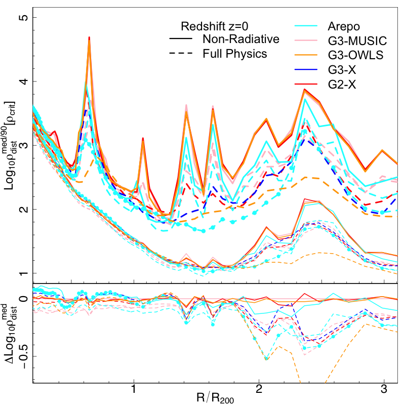
Figure 4: Radial profiles of median and $90^{\rm th}$ percentile gas density ($\rho_{\rm dist}^{\rm med}$, lower curves; and $\rho_{\rm dist}^{90}$, upper curves) at $z$=0, deduced from the distribution of gas densities within the spherical shells used in Figure 2. As before, we show results for non-radiative and full physics runs (solid and dashed curves respectively), and radii are normalised to $R_{200}$. In the lower panel, for clarity, we focus on the residuals of each of the median profiles with respect to the G3-MUSIC non-radiative run. Note that we distinguish between the two sets of full physics Arepo and G3-MUSIC runs as in Figure 2.

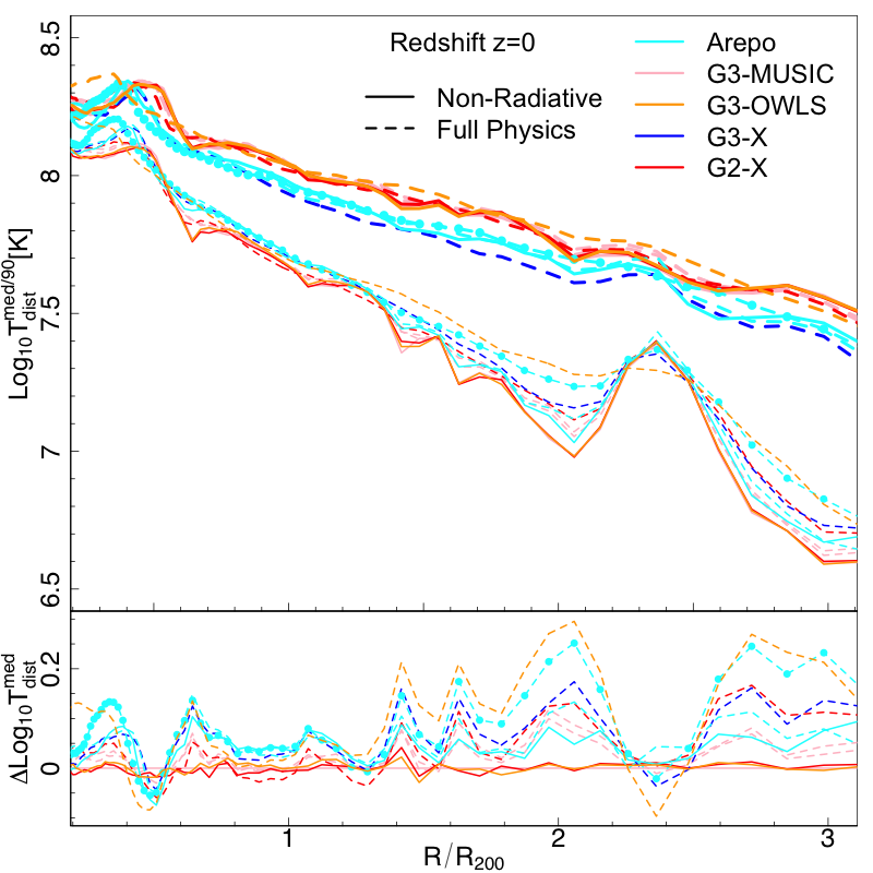
Figure 5: Radial profiles of median and $90^{\rm th}$ percentile gas temperature ($T_{\rm dist}^{\rm med}$, lower curves; and $T_{\rm dist}^{90}$, upper curves) at $z$=0, deduced from the distribution of internal energies within the spherical shells used in Figure 2. As in Figure 4, we consider only the residuals of the median profiles with respect to the G3-MUSIC non-radiative run, and we distinguish between the two sets of full physics Arepo and G3-MUSIC using the same convention.

An instructive alternative to spherically averaging profiles is to consider measures of the distribution of values within each spherical shell, as explored in Zhuravleva et al. (2013) and subsequent papers. In Figure 4, we show how the median (lower curves) and $90^{\rm th}$ percentile values (upper curves) of gas density, $\rho_{\rm dist}^{\rm med}$ and $\rho_{\rm dist}^{90}$, vary with radius. Here the gas density is the intrinsic value (for a particle or cell) tracked in the simulation. We find that the median profile ($\rho_{\rm dist}^{\rm med}$) and the corresponding spherically averaged profile in Figure 2 are in very good agreement within $R_{200}$, at the $5-10\%$ level.

The enhancement in $\rho_{\rm dist}^{\rm med}$ apparent at $R\simeq 2\,R_{200}$ is consistent across codes and galaxy formation models, but its magnitude differs between non-radiative and full physics runs by $\sim 30$ per cent. We associate this with substructure infalling along the cosmic web, evident in the upper right quadrants of the upper panels in Figure 1. At $R\leq R_{200}$, pronounced enhancements are apparent in $\rho_{\rm dist}^{90}$; the locations of these peaks are broadly consistent between codes and galaxy formation models, albeit with significant scatter in magnitude. We find the stronger enhancements in the non-radiative runs (for the reasons already discussed), but the larger scatter (by a factor of $\sim 10$ in the enhancement at $\sim 0.6\,R_{200}$) in the full physics runs. As noted by Zhuravleva et al. (2013) and e.g. Avestruz, Nagai & Lau (2016), these are naturally interpreted as signatures of substructure.

Figure 5 shows that the density enhancement in Figure 4 at $R\simeq 2\,R_{200}$ has a corresponding temperature enhancement, which is most easily discernible in the median profile ($T_{\rm dist}^{\rm med}$, lower curves) and is most sharply defined in the non-radiative runs (again, for the reasons already discussed). The enhancement evident in the spherically averaged temperature profile at $\sim 0.5-0.6R_{200}$ is also apparent in $T_{\rm dist}^{\rm med}$ and $90^{th}$ percentile temperatures profile ($T_{\rm dist}^{90}$, upper curves), while smaller features are evident at the locations of the density enhancements in Figure 4. The sharpness of these features varies systematically between non-radiative runs, which are in very good agreement with each other, and the full physics runs, which tend to produce less sharply defined features than in the non-radiative runs.

We have used snapshots finely spaced over the redshift range $z$=0.5 to $z$=0 to verify that the temperature enhancements within $R_{200}$ evident in these radial profiles occur frequently during the cluster’s assembly. This strengthens our assetion that they are transient features whose position moves to smaller radii over a dynamical time, consistent with the motions of substructures whose passage shocks the ICM. In contrast, the feature at $\sim(2-3)\,R_{200}$ identified at $z$=0 varies in amplitude but has remained at approximately $\sim(2-3)\,R_{200}$ since $z$=0.5, which we argue is associated with gas inflow and substructure motion in the cosmic web (see, e.g., Burns et al., 2010).

We note that Avestruz, Nagai & Lau (2016) considered the mean mass-weighted temperature of the ICM at larger radius (defined relative to $R_{500}$, the radius enclosing a mean density of 500 times critical density) of an ensemble average of clusters and found that the presence of substructure tended to reduce it compared to the temperature when substructure was excluded, as a result of the cooler gas associated with substructures bringing down the average temperature. This is consistent with our results - we consider the temperature distribution of all gas within the shell, and so the $90^{\rm th}$ percentiles will include the contributions of shocked gas, some of which can be associated with the $90^{\rm th}$ percentiles in density. We have verified that excluding overdense gas leads to an increase in the mass weighted average temperature within shells, albeit our result is noisier than that of Avestruz, Nagai & Lau (2016).

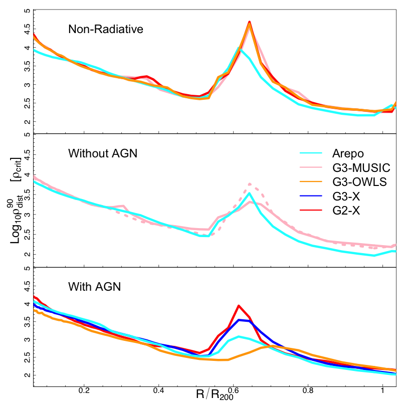
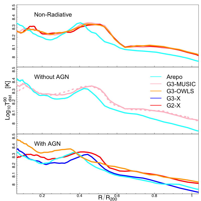
Figure 6: Radial profiles of the $90^{\rm th}$ percentile gas density (top panels) and temperature (bottom panels), computed as in Figures 4 and  5. We distinguish between non-radiative runs (upper panel) and full physics runs “Without AGN” and “With AGN” (middle and lower panels, respectively). As before, there are two full physics G3-MUSIC runs without AGN - G3-MUSIC-SH and G3-MUSIC-PS - which we distinguish by heavy and light dashed curves, while there while there is one Arepo full physics run with AGN and one without.

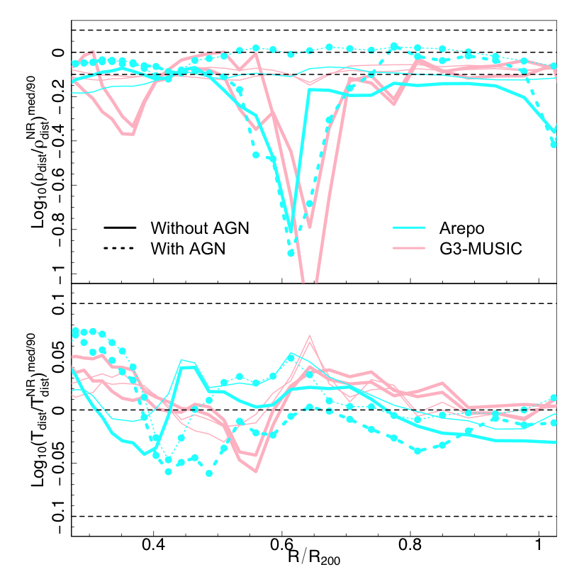
Figure 7: Comparison of density and temperature profiles in the Arepo and G3-MUSIC simulations, for which we have multiple full physics models, as in Figures 4 and  5. These profiles are scaled by the density and temperature profiles in the corresponding non-radiative runs. Light (heavy) curves are based on the medians ($90^{\rm th}$ percentiles), while we distinguish between runs “Without AGN” (the two G3-MUSIC runs and one of the Arepo runs) and “With AGN” (the other Arepo run) by using solid and dashed curves; for emphasis, we also overlay filled circles on the “With AGN” curves. Horizontal dashed lines delineate $\pm 25\%$.

How might different physical processes modelled in the simulations impact radial density and temperature profiles? In Figure 6, we investigate how these profiles are influenced by the physical processes modelled in the simulation, focusing on the $90^{\rm th}$ percentile values of the density and temperature distributions within spherical shells where we expect differences between the simulations to be most marked. Here we group the simulations into (1) non-radiative runs, and full physics runs (2) with, and (3) without AGN. Note that we zoom in on the radial range $0.1\leq R/R_{200}\leq 1$ to assess the extent to which the physics of galaxy formation - particularly AGN feedback - might affect the ICM outside of where the central cluster galaxy resides.

(1) Non-radiative Case: We see a sharply peaked density enhancement at $\sim 0.6R_{200}$, evident in all but one of the runs, which is most pronounced in the non-radiative runs. There is excellent agreement between the classic SPH codes (G3-MUSIC, G2-X, and G3-OWLS) - unsurprising, given that they are variants of GADGET2/3 (Springel, 2005) with the same gravity solver and the treatment of SPH - while Arepo underpredicts the magnitude of the density enhancement in comparison, but otherwise tracks the predictions of the classic SPH codes. Similarly, there is excellent consistency between the temperature profiles predicted by the classic SPH codes, which show an enhancement at $\sim 0.5R_{200}$, whereas Arepo underpredicts the temperature across most of the radial range, while the enhancement is offset to $\sim 0.4R_{200}$. Note that the Arepo density and temperature profiles begin to peel away from their classic SPH counterparts at $\sim 0.1R_{200}$, as we expect because of the difference in hydrodynamics solvers (e.g. Sembolini et al., 2016a).

(2) Full Physics without AGN Case: The trends evident in the non-radiative runs are also apparent in the full physics runs without AGN - Arepo-SH, G3-MUSIC-SH, and G3-MUSIC-PS. The amplitude of the density enhancement at $\sim 0.6R_{200}$ is reduced relative to in the non-radiative runs, and we see from the G3-MUSIC that the assumed stellar feedback model has an impact.

(3) Full Physics with AGN Case: The amplitude of the density enhancement at $\sim 0.6R_{200}$ shows considerable variation between the different full physics runs that implement AGN feedback, with the two classic SPH codes G2-X and G3-OWLS bracketing the range of variation - the enhancement is peaked in G2-X, whereas it is effectively smoothed away in G3-OWLS. A similar range of variation is evident in the temperature profiles, with the amplitude, sharpness, and, in particular, the location of the peak of the temperature enhancement at $\sim 0.5R_{200}$; for example, the enhancement in the G3-OWLS run peaks at $\sim 0.35R_{200}$, compared to $\sim 0.45R_{200}$ in the G2-X and G3-X runs. Interestingly, the classic SPH runs predict systematically higher temperatures across most of the radial range when compared to the modern SPH run with G3-X and Arepo.

These observations show that the physical processes modelled in a simulation can influence the ICM density and temperature radial profiles at larger radii, but the most significant differences are associated with the density and temperature enhancement associated with substructure. Where we see systematic differences - for example, in the temperature profiles in the “With AGN” runs - these can be attributed to expected differences between classic SPH on the one hand, and modern SPH and Arepo on the other.

To isolate the particular effect of feedback on the ICM density and temperature radial profiles, in Figure 7 we look at the profiles in the Arepo-SH and Arepo-IL runs, which are run without and with AGN feedback, and in the G3-MUSIC-SH and G3-MUSIC-PS, which are run without AGN feedback but utilise two different stellar feedback models (cf. Springel & Hernquist, 2003; Piontek & Steinmetz, 2011). We show logarithmic differences with respect to the non-radiative counterparts, and plot medians (light curves) and $90^{\rm th}$ percentiles (heavy curves) in the radial range $0.3\leq R/R_{200}\leq 1$; models with AGN are indicated by dotted curves overlaid with filled circles. The light dashed horizontal lines indicate $\pm 25\%$ with respect to the non-radiative run. As we would expect, the logarithmic difference is dominated by the density enhancement at $\sim 0.6R_{200}$; logarithmic differences in the temperature profiles are small ($\lesssim 0.05$ dex), while the corresponding differences in density are predominantly $\lesssim 0.1$ dex, although these increase where we see enhancements that we associated with substructure.

In Figure 8, we shift focus to the radial velocity profile of gas within the cluster, reasoning that features in the temperature profile are a response to gravitational and hydrodynamical influences; namely, shocks. Here we show the variation of spherically averaged radial velocity of gas with radius, with radii normalised to $R_{200}$ while radial velocities are in units of km/s; $v_{\rm rad}\!<\!0\,(>\!0)$ implies inflow (outflow). For a system in hydrodynamic equilibrium, we would expect $\langle v_{\rm rad}\rangle\simeq 0$, but instead we see a pronounced dip to $\sim-500\,{\rm km}{\rm s}^{-1}$ at $\sim 0.7\,R_{200}$, before a sharp rise to $\sim 400\,{\rm km}{\rm s}^{-1}$ peaking at $\sim 0.5\,R_{200}$. There is appreciable variation between the runs, but the trend is systematic.

Interestingly, we see a feature in the dark matter radial velocity (heavy dotted-dashed curve), similar to the feature evident in the gas radial velocity, albeit smaller in amplitude and displaced outwards in radius. At radii $R\gtrsim r_{200}$, we see substantial differences between runs of $\sim\!200$ km/s. It is noteworthy that the unstructured mesh code, Arepo, and the modern SPH code, G3-X, predict systematically more negative radial velocities than the other codes, which are based on classic SPH, which are in broad agreement with one another. Strikingly, the dark matter radial velocity profile more negative than the gas radial velocity profiles by $\sim 200-400$ km/s, but there are common features across the various profiles (for example, the bump at $\sim\!2\!R_{200}$).

In Figure 9, we provide an estimate for the strength of the shocks in the cluster gas by calculating the spherically averaged Mach number of gas as a function of cluster-centric distance. There are several approaches that we could take to estimating where and when shocks occur, which include tracking spatially localised jumps in temperature and/or velocity (e.g. Vazza, Brunetti, & Gheller, 2009), which are relatively straightforward in mesh-based codes where there are well-defined boundaries between cells; or tracking jumps in entropy or internal energy over time (Keshet et al., 2003), which is particularly straightforward in particle-based codes. However, we follow Mohapatra & Sharma (2019) and use the root-mean-square (rms) Mach number,

$$M_{\rm rms}=\frac{\sqrt{\langle{v^{2}}\rangle}}{c_{s}},$$ (3)

where $\langle{v^{2}}\rangle$ is the rms velocity computed for all gas elements (particles or cells) within a spherical shell, and $c_{s}$ is the sound speed, which we compute directly from the internal energies.

As we would expect, the locations of features in the spherically averaged temperature and radial profiles correlate with features in the rms Mach number radial profile. The magnitude of $M_{\rm rms}$ is larger in the moving-mesh Arepo runs - both the non-radiative and full physics variants - and in the modern SPH G3-X run, compared to the classic SPH runs, in the regime of stronger shocks, where $M_{\rm rms}\gtrsim 2$ and $R\gtrsim{1.5}R_{200}$, by between 10% and 25%. The trend is for the average rms Mach number to increase with cluster-centric distance, with values of $M_{\rm rms}\lesssim{1}$ within $0.5\,R_{200}$ and $M_{\rm rms}\lesssim{1.8}$ within $R_{200}$, rising to $M_{\rm rms}\lesssim{3-4}$ at $3\,R_{200}$. Note, however, that these numbers are indicative - if, instead, we measure median ($90^{\rm th}$ percentiles) values of $\langle{v^{2}}\rangle$ within each shell, we find $M_{\rm rms}\lesssim{2}(3)$ within $R_{200}$ and $M_{\rm rms}\lesssim{5}(50)$ at $3\,R_{200}$. Nevertheless, the values are broadly consistent with reported values in the literature. For example, Vazza, Brunetti, & Gheller (2009) note that “internal shocks” within the virialised region of a cluster tend to have Mach numbers of $M\lesssim 3$, with occasional spikes as a result of mergers, while “external shocks” tend to be much stronger and larger ($M\gg{10}$), arising from accretion onto filaments and sheets (see also Miniati, et al., 2001).

We have demonstrated that enhancements in gas density and temperature profiles within $R_{200}$, as well as features in gas and dark matter radial velocity profiles, plausibly correspond to substructures evident in projected gas density and temperature maps (Figure 1). We now investigate how substructure gives rise to the features in detail.

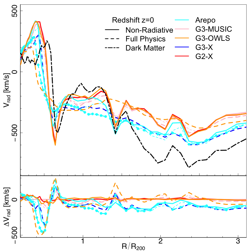
Figure 8: Spherically averaged radial velocity profiles at $z$=0. In the upper panel, we show the spherically averaged radial velocity profiles measured in the non-radiative runs (solid curves) and full physics runs (dashed curves). Velocities are expressed in units of km/s, while we normalise radii by $R_{200}$ as before. For reference, we show by the heavy dotted-dashed curve the dark matter radial velocity profile as found in the G3-MUSIC non-radiative run. In the lower panel, we show the residuals of each of these profiles with respect to the G3-MUSIC non-radiative run again.

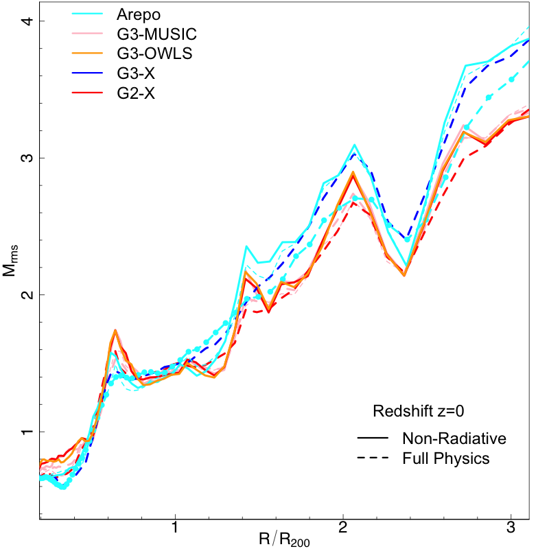
Figure 9: Spherically averaged radial profiles of the root-mean-square Mach number, $M_{\rm rms}$, at $z$=0. As before, we show results from the non-radiative runs (solid curves) and full physics runs (dashed curves), and radii are normalised by $R_{200}$ as before.

3.2 The impact of substructure dynamics on the ICM

So far we have identified the imprint of substructure on the radial profiles of the ICM gas density, temperature, and radial velocity; we now shift our focus to the substructure population and investigate how its dynamical effects impact the ICM.

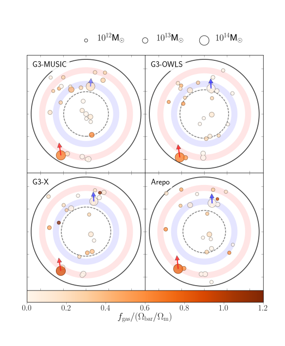
Figure 10: Projected spatial distribution of haloes within $1.25R_{200}$ of the cluster. We include only those haloes with masses $\geq 10^{12}h^{-1}{\rm M}_{\odot}$. Symbol size and colour scale with mass and gas fraction, with lighter hues indicating gas paucity and dark hues indicating gas richness. The virial radius $R_{200}$ is represented by the solid circle, the radius at which the underlying cluster halo circular velocity profile reaches its maximum by the dashed circle, while the shaded regions indicate the inner and outer boundaries of the temperature and radial velocity profile features.

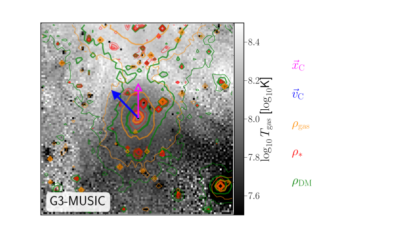
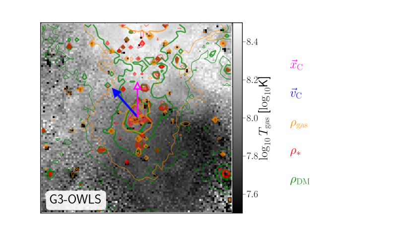
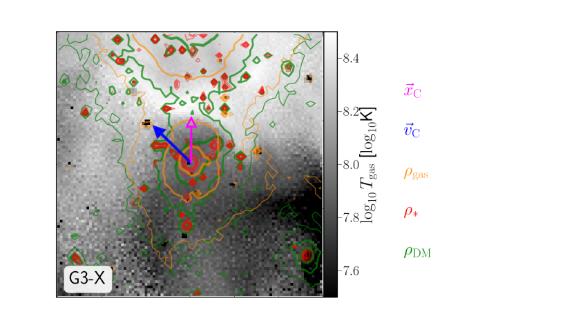
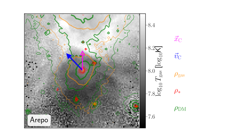
Figure 11: Infalling group shock in a subset of the full physics runs; from top right to bottom left, G3-MUSIC, G3-OWLS, G3-X, and Arepo. Here we zoom in on a region $2.1h^{-1}{\rm Mpc}$ wide and $1.1h^{-1}{\rm Mpc}$ thick, centred on and in the orbital plane of the galaxy group that generates the shock that gives rise to the feature in the temperature profile at $0.9R_{200}$. We show the mean logarithmic temperature distribution along the line of sight in this slab in grayscale, where each pixel is $20$ kpc in size. We show also contour maps of the average dark matter density in green; the average gas density in orange; and the average stellar density in red. The galaxy group’s direction of motion relative to the cluster’s centre-of-mass is shown by a blue arrow, while the direction towards the cluster centre is shown by by a magenta arrow.

In Figure 10 we show the projected spatial distribution of haloes of mass $M_{\rm 200}\geq 10^{12}h^{-1}{\rm M}_{\odot}$ and within $1.25R_{\rm 200}$ of the cluster’s centre in the full-physics simulations. Symbol size is proportional to halo mass, while symbol colour indicates gas fraction. The solid outermost circle represents the cluster’s radius $R_{\rm 200}$, while the dashed circle indicates the position of the peak of the circular velocity profile. The shaded regions mark the outer and inner bounds of the features identified in the spherically averaged temperature and radial velocity profiles (cf. Figures 3 and 8).

The most striking feature of Figure 10 is the presence of two distinct massive substructures whose radial distances coincide with features in the gas radial velocity profile. As a case study, we investigate these substructures in more detail. Their trajectories are consistent with the trends we see in the radial velocity profiles - the outer, gas-rich substructure is infalling with a velocity $\sim-1700$ km/s, whereas the inner, gas-poor substructure is moving outwards with a velocity $\sim 1500$ km/s - although their velocities are much higher than the spherically averaged velocities at these radii, and supersonic. Their velocity vectors are relatively well aligned, with an angle between them of $\sim$$20^{\circ}$, and their direction of motion aligns with the orientation of the large-scale filaments within which the cluster is embedded (see further discussion in § 3.3).

These results are consistent with non-radiative and dark matter only versions of these simulations, which we check by cross-matching halos identified in the full physics run with those in the non-radiative and dark matter only runs, and confirm excellent agreement between the spatial and kinematic distributions. Differences that we note in the dark matter only run – that the counterpart to the outgoing halo is at a slightly larger cluster-centric distance than in the full physics and non-radiative runs – can be readily understood as a consequence of the change in bound mass arising from the stripping of its gas content.

In Figure 11, we make explicit how the infalling substructure, highlighted in Figure 10, impacts the ICM. Recall that this infalling substructure is gas-rich ($f_{g}\sim(0.7-0.9)\Omega_{b}/\Omega_{m}$), and it has a large radial velocity ($\sim$-1700km/s) relative to the cluster; this velocity is significantly larger than the motions of cluster particles in the same region – for dark matter, $\left\langle v_{r}\right\rangle\sim-150$ km/s with dispersions of $\sim 1000$ km/s; for gas $\left\langle v_{r}\right\rangle\sim-250$ km/s, with dispersions of $\sim 600$ km/s. We plot the projected gas distribution, weighted by temperature, in a region $2.1h^{-1}{\rm Mpc}$ wide and $1.1h^{-1}{\rm Mpc}$ thick, centred on and in the orbital plane of the substructure. Contours indicate dark matter, gas, and stellar density associated with the substructure, while arrows show the direction to the cluster centre ($\vec{x}_{\rm C}$) and the direction of motion of the substructure relative to the cluster centre ($\vec{v}_{\rm C}$).

Figure 11 shows that the infalling substructure driving a shock into the ICM - there is evidence for shocked gas in advance of the substructure and trailing gas in its wake in all of the runs. The temperature enhancement associated with the shock is more pronounced in the direction of the cluster centre, towards which the density gradient is higher, than in the direction of motion.

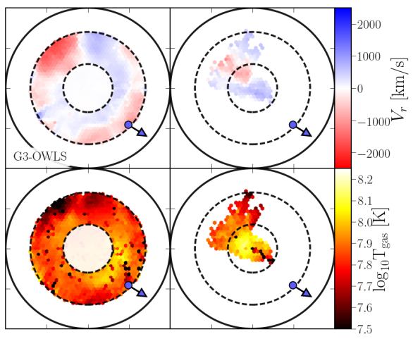
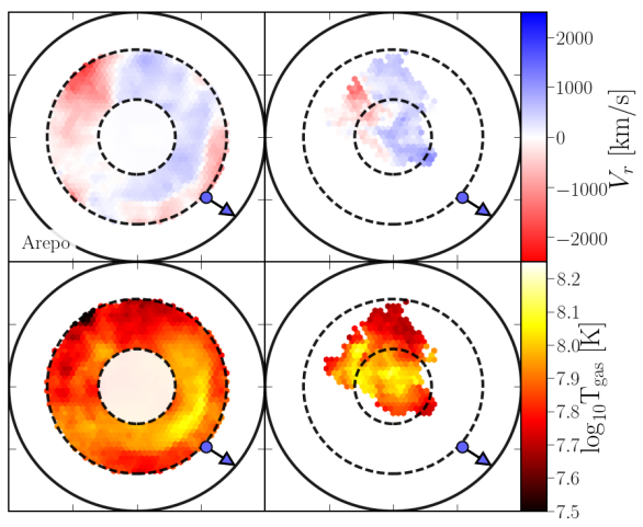
Figure 12: Gas properties around the inner shock in the G3-OWLS and Arepo full physics runs (upper and lower panels, respectively). We show, in projection, the mean radial velocity (upper panels) and temperature (lower panels) of gas in a shell around the shock feature (left panels) and the gas stripped from the outward going substructure (right panels) in the Arepo full physics run. We show also the position of the outward moving substructure and its direction of motion, with the point and arrow colour coded according to its radial velocity. The outer solid circle is at $R_{200}$, while the inner/outer dashed circles are at $0.4/0.8R_{200}$ and encompass the inner shock. For clarity, we do not include gas interior to the shell in projection.

That a fast-moving, infalling, gas-rich substructure might generate a shock in the ICM is not surprising; but what is the influence of the gas-poor substructure moving outwards? At $z$=0, it is moving with a radial velocity of $\sim$1500 km/s; however, its position and velocity do not correspond to the inner feature seen in the temperature and radial velocity profiles – its radial velocity is too high, and it is at too great a clustercentric radius. By tracking its orbit to earlier times, we can say that it had a mass on infall of $\sim 6\times 10^{13}$ M_⊙ and it was gas-rich. At its pericentric passage of $\sim 0.15\,R_{200}$, it deposited a gas mass of $\sim 8\times 10^{12}$ M_⊙ in $\sim 50$ Myrs as it moved at speeds of $\sim 2750$ km/s, and led to its baryon fraction plummeting from $\gtrsim 0.5\Omega_{b}/\Omega_{m}$ to $\ll\Omega_{b}/\Omega_{m}$. It is this stripping event and the gas associated with it that produces the shock at $\sim(0.5-0.6)R_{200}$.

To illustrate these observations, in Figure 12 we show the projected radial velocities and temperatures (upper and lower panels respectively) of gas in the vicinity of the inner temperature enhancement (left panels), and gas stripped from the outward moving substructure (right panels). To show the generality of our results and the consistency between code behaviour, we consider two representative cases - G3-OWLS at the top, and Arepo at the bottom. Inspection of the left panels makes clear an arc of shock heated gas, both trailing the outwardly moving substructure and colliding with infalling gas; the right panels reveal that the shocked cluster gas is propelled outwards by the cold, dense, fast moving gas stripped from the outwardly moving cluster. The fastest outwardly moving portion of this stripped gas is spatially coincident with the inner edge of the shock, pushing material in front of it, and it is this outwardly moving wake that shock heats when it encounters infalling gas.

3.3 The role of the cosmic web

A consistent feature of the results in § 3.1 is the presence of an enhancement in gas density and temperature at $\sim(2-3)\,R_{200}$. In contrast to the transient enhancements with $R_{200}$, this feature is long-lived and we have argued that it is likely associated with gas accretion from the cosmic web. We have also demonstrated that the massive substructures whose passage through the ICM drives shocks have been accreted onto the cluster from a preferential direction, which we interpreted as a signature for infall along filaments.

We use DisPerSe (cf. Sousbie, 2011) to characterise filamentary structure in the vicinity of the cluster. DisPerSe computes a discrete density field from a Delaunay tessellation of particles and identifies filaments as ridges connecting maxima through saddle points in the underlying density field. The result is a “skeleton” of the density field, consisting of a fully connected network of segments, which can be smoothed (by pairwise averaging of neighbouring segments) to focus on a given spatial scale. Here we compute the skeleton using both dark matter and gas in cubes of size 4 and 20 $h^{-1}$ Mpc on a side, centered on the location of the maximum density of the cluster.

Figure 13 gives a visual impression of the cosmic web in which the cluster is embedded. Solid red lines show a $3h^{-1}{\rm Mpc}$ wide slice of the network of filaments with a persistence threshold $c$=0.01 in a $20\,h^{-1}{\rm Mpc}$ cube smoothed onto a $128^{3}$ mesh, consecutively trimmed of arcs with robustness smaller than the mean plus 1 standard deviation and smoothed over a $3h^{-1}{\rm Mpc}$ spatial scale. While these results are calculated for the gas, we note that we recover a very similar skeleton on large scales using the dark matter density. Dashed circles indicate the locations of the features in the radial velocity profiles, while the solid circles correspond to the gas-poor outwardly moving substructure (lower in $x$-$y$, left in $y$-$z$) and gas-rich infalling substructure respectively.

The result is visually striking - Figure 13 makes clear how the trajectories of both substructures can be traced to larger-scale filaments, while also highlighting the connection between the enhancements in gas densty and temperature, as well as the spherically averaged negative radial velocity, at $\sim(2-3)\,R_{\rm 200}$, to the merging of several smaller filaments along the direction of the most robust one. This explains why the location of this feature should be long-lived, albeit varying in magnitude, whereas the shocks associated with infalling substructures within $R_{200}$ should be short-lived and dynamic.

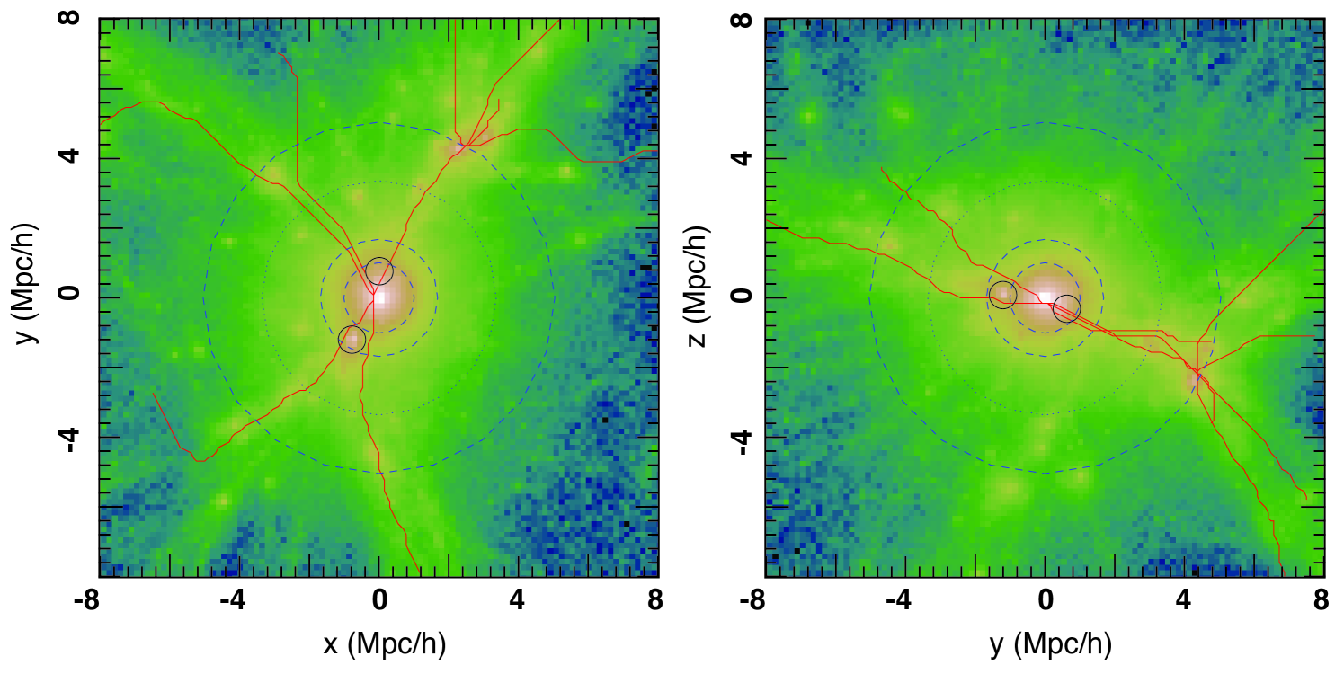
Figure 13: Large-scale cosmic web connectivity in G3-OWLS. Projected gas density centred on the cluster within a $3\,R_{\rm 200}$ thick slice in the $x$-$y$ (left panel) and $y$-$z$ (right panel) planes, colour-coded by the logarithm of the density. As described in the text, the solid red lines show the network of filaments recovered by DisPerSe (cf. Sousbie, 2011) while the dashed circles indicate the locations of features evident in the spherically averaged radial velocity profiles, and solid circles correspond to the two massive substructures investigated in the previous subsection.

4 Summary

We have used a suite of cosmological hydrodynamical zoom simulations of a single galaxy cluster, run with a range of astrophysical codes and galaxy formation models as part of the nIFTy comparison project (see Sembolini et al., 2016a, b), to study how the thermodynamical properties of the intra-cluster medium (ICM) in a galaxy cluster’s outskirts ($0.3\leq R/R_{200}\lesssim 3$) at $z$=0 are influenced by the accretion of substructure from the cosmic web. Using the radial profiles of gas density, temperature, and radial velocity, we highlighted the presence of enhancements in gas density and temperature, which we noted are associated with shocks (as measured by the Mach number) and which are commonly interepreted as signatures of the passage of substructure (see, e.g., Zhuravleva et al., 2013; Lau et al., 2017). We showed how such features within $R_{200}$ can be linked to substructure evident in projected gas density and temperature maps, and can be connected to the passage of substructures through the ICM.

In particular, we looked in detail at two massive substructures - one gas-rich substructure infalling on a preferentially radial orbit with a relative speed of $-1700$km/s, producing the clear signature of a shock in the direction of its motion; the other gas-poor substructure, moving outwards with a velocity of $1500$km/s, and gravitationally influencing gas in its vicinity. By constructing the cosmic web in the vicinity of the cluster, we established that the cluster accretes from two dominant filaments, but that a network of filaments combine at $\sim(2-3)\,R_{200}$ to give rise to density and temperature enhancements, associated with the infall of gas and dark matter along the cosmic web. Because the trajectories followed by the substructures that give rise to the shocks within $R_{200}$ are fixed by the filaments from which they were accreted, this suggests a way to reconstruct the infall time and direction of massive substructures from observational data (e.g. radio sychrotron measurements of termination shocks associated with the infalling galaxy substructures Brown & Rudnick, 2011).

We note general qualitative agreement between the selection of astrophysical codes and galaxy formation models (non-radiative and full physics) used in this paper in terms of their recovery of spherically averaged cluster gas profiles, at the level of $\sim 25\%$ or 0.1 dex between runs. Over the radial range $0.3\,R_{200}\leq R\lesssim R_{200}$, we find broad agreement between predictions for the locations of enhancements in gas density and temperature, and when and where shocks occur, but differences between predictions for the sizes of enhancements and how strong shocks - as gauged by the root-mean-square Mach number, $M_{\rm rms}$ - should be, most notably between full physics runs. This is as we would expect. Both gas and substructure accretion onto the cluster will be driven by the large-scale gravitational field, which dictates when and where, and we expect excellent agreement between the codes because of our requirement that they are aligned (cf. Sembolini et al., 2016a), whereas shock strength will be driven by a number of factors, including resolution and choice of hydro solver, and so we expect greater variation between codes.

Although we have considered only a single galaxy cluster, albeit multiple realisations with different codes and galaxy formation models, our results imply that the dynamical effects of accreting substructure on ICM properties will need to be accounted for when making accurate predictions for next generation surveys, such as e.g. the Square Kilometre Array in the radio continuum, tracing synchrotron emission (e.g., Giovannini et al., 2015; Vazza et al., 2015), and eRosita (e.g., Merloni et al., 2012), X-Ray Imaging and Spectroscopy Mission (XRISM) (e.g., Tashiro et al., 2018), and ATHENA (e.g., Nandra et al., 2013) in X-ray. Conversely, these surveys can open up a new view of the merger and accretion histories of clusters.

In summary, we have investigated in detail how the passage of massive substructures influence the ICM at large cluster-centric radius and shown how it connects to features in radial ICM profiles, which previously have been quantified in a statistical sense (e.g., Zhuravleva et al., 2013; Rasia et al., 2014; Nelson et al., 2014; Lau et al., 2015; Ota, Nagai & Lau, 2018; Zinger et al., 2018). Our case study of the two massive substructures shows that the manner in which such systems drive shocks into the ICM is not uniform; in one case, we have the classical picture of a gas-rich, infalling, substructure driving a shock, while in the other, it is stripped gas, which was once associated a now gas-poor, outgoing, substructure, is driving a shock. Finally, we have verified that the predictions of different astrophysical codes and galaxy formation models are in broad agreement, predicting spherically averaged radial properties of the ICM that agree at the 25% (0.1 dex) level.

Appendix A Simulation codes

Arepo

(Puchwein)

The basic Arepo code (cf. Springel, 2010) utilises a TreePM gravity solver and a finite-volume Godunov scheme on an unstructured moving Voronoi mesh to solve the equations of hydrodynamics. Two galaxy formation prescriptions are used in the full physics runs; the first (Arepo-IL) is used in the Illustris Simulation, includes AGN feeding and feedback, and is described in Vogelsberger et al. (2013, 2014). The second (Arepo-SH) uses the standard Springel & Hernquist (2003) scheme, without AGN, and matches that used in G3-MUSIC.

G2-X

(Kay)

G2-X is built on the public version of GADGET2 (Springel, 2005), using the standard cubic spline kernel with 50 neighbours. The adopted galaxy formation prescription is descrived in detail in Pike et al. (2014), but it can summarised as follows; radiative cooling follows the Thomas & Couchman (1992) prescription; stars form following Schaye & Dalla Vecchia (2008) at a rate fixed by the Schmidt-Kennicutt relation (Kennicutt, 1998), and produce feedback using a prompt thermal Type II supernova model; and the modelling of AGN feeding and feedback is based on Booth & Schaye (2009).

G3-MUSIC

(Yepes)

G3-MUSIC is built on GADGET3, which derives from the public version of the GADGET2 code of Springel (2005), with improvements in time-stepping and domain decomposition. It employs the entropy-conserving formulation of SPH described in Springel & Hernquist (2002), with a spline kernel (Monaghan & Lattanzio, 1985) and artificial viscosity as modelled in Monaghan (1997). It uses two models - the standard Springel & Hernquist (2003) scheme (G3-MUSIC-SH) and the Piontek & Steinmetz (2011) scheme (G3-MUSIC-PS) - neither of which include AGN, in the full physics runs.

G3-OWLS

(McCarthy, Schaye)

G3-OWLS is built on GADGET3 and employs the standard entropy-conserving SPH scheme of Springel & Hernquist (2002) with a cubic spline kernel of 48 neighbours. The galaxy formation prescription used in the full physics run is presented in extensive detail in Schaye & Dalla Vecchia (2008), Dalla Vecchia & Schaye (2008), Wiersma et al. (2009a), Booth & Schaye (2009), Wiersma et al. (2009b), Schaye et al. (2010), and encompasses modelling of radiative cooling, star formation, stellar evolution, stellar feedback, and AGN feeding.

G3-X

(Murante, Borgani, Beck)

G3-X is built on GADGET3 and developed by (Beck et al., 2016) to include a Wendland $C^{4}$ kernel with 200 neighbours (cf. Dehnen & Aly, 2012), artificial conductivity to promote fluid mixing following Price (2008) and Tricco & Price (2013), but with an additional limiter for gravitationally induced pressure gradients. The full physics run adopts the cooling prescription of Wiersma et al. (2009a); heating via a uniform UV background as in Haardt & Madau (2001); star formation and chemical evolution as in Tornatore et al. (2007); stellar feedback in the form of supernovae as in Springel & Hernquist (2003); and AGN feedback as in Steinborn et al. (2015).

References

- Avestruz, Nagai & Lau (2016) Avestruz C., Nagai D., Lau E. T., 2016, ApJ, 833, 227
- Bailin & Steinmetz (2005) Bailin, J., & Steinmetz, M. 2005, ApJ, 627, 647
- Beck et al. (2016) Beck, A. M., Murante, G., Arth, A., et al. 2016, MNRAS, 455, 2110
- Benitez-Llambay (2015) Benitez-Llambay, A., 2015, py-sphviewer: Py-SPHViewer v1.0.0, Zenodo 10.5281/zenodo.21703
- Biffi et al. (2014) Biffi, V., Sembolini, F., De Petris, M., et al. 2014, MNRAS, 439, 588
- Booth & Schaye (2009) Booth C. M., Schaye J., 2009, MNRAS, 398, 53
- Brown & Rudnick (2011) Brown, S., & Rudnick, L. 2011, MNRAS, 412, 2
- Burns et al. (2010) Burns, J. O., Skillman, S. W., & O’Shea, B. W. 2010, ApJ, 721, 1105
- Chen et al. (2019) Chen H., Avestruz C., Kravtsov A. V., Lau E. T., Nagai D., 2019, arXiv e-prints, arXiv:1903.08662
- Cui et al. (2016) Cui, W., Power, C., Knebe, A., et al. 2016, MNRAS, 458, 4052
- Cui, et al. (2018) Cui W., et al., 2018, MNRAS, 473, 68
- Dalla Vecchia & Schaye (2008) Dalla Vecchia C., Schaye J., 2008, MNRAS, 387, 1431
- Davé et al. (2001) Davé R., et al., 2001, ApJ, 552, 473
- Dehnen & Aly (2012) Dehnen, W., & Aly, H. 2012, MNRAS, 425, 1068
- Durret et al. (2016) Durret, F., Márquez, I., Acebrón, A., et al. 2016, A&A, 588, A69
- Elahi, Thacker, & Widrow (2011) Elahi P. J., Thacker R. J., Widrow L. M., 2011, MNRAS, 418, 320
- Elahi et al. (2013) Elahi P. J., et al., 2013, MNRAS, 433, 1537
- Elahi et al. (2019) Elahi, P. J., et al. 2019, eprint arXiv:1902.01010
- Ghirardini, et al. (2018) Ghirardini V., et al., 2018, A&A, 614, A7
- Giovannini et al. (2015) Giovannini G., et al., 2015, Proceedings of Advancing Astrophysics with the Square Kilometre Array (AASKA14). 9 -13 June, 2014. Giardini Naxos, Italy
- Haardt & Madau (2001) Haardt, F., & Madau, P. 2001, Clusters of Galaxies and the High Redshift Universe Observed in X-rays,
- Hao et al. (2011) Hao J., Kubo J. M., Feldmann R., Annis J., Johnston D. E., Lin H., McKay T. A., 2011, ApJ, 740, 39
- Hoeft et al. (2008) Hoeft, M., Brüggen, M., Yepes, G., Gottlöber, S., & Schwope, A. 2008, MNRAS, 391, 1511
- Kennicutt (1998) Kennicutt, R. C., Jr. 1998, ApJ, 498, 541
- Keshet et al. (2003) Keshet, U., Waxman, E., Loeb, A., Springel, V., & Hernquist, L. 2003, ApJ, 585, 128
- Keshet et al. (2004) Keshet, U., Waxman, E., & Loeb, A. 2004, ApJ, 617, 281
- Klypin et al. (2001) Klypin, A., Kravtsov, A. V., Bullock, J. S., & Primack, J. R. 2001, ApJ, 554, 903
- Knebe et al. (2004) Knebe, A., Gill, S. P. D., Gibson, B. K., et al. 2004, ApJ, 603, 7
- Komatsu & Seljak (2001) Komatsu, E., & Seljak, U. 2001, MNRAS, 327, 1353
- Komatsu et al. (2011) Komatsu, E., Smith, K. M., Dunkley, J., et al. 2011, ApJS, 192, 18
- Kravtsov & Borgani (2012) Kravtsov A. V., Borgani S., 2012, ARA&A, 50, 353
- Lau et al. (2015) Lau E. T., Nagai D., Avestruz C., Nelson K., Vikhlinin A., 2015, ApJ, 806, 68
- Lau et al. (2017) Lau E. T., Gaspari M., Nagai D., Coppi P., 2017, ApJ, 849, 54
- Lewis et al. (2000) Lewis G. F., Babul A., Katz N., Quinn T., Hernquist L., Weinberg D. H., 2000, ApJ, 536, 623
- Makino et al. (1998) Makino, N., Sasaki, S., & Suto, Y. 1998, ApJ, 497, 555
- Mantz et al. (2014) Mantz, A. B., Allen, S. W., Morris, R. G., et al. 2014, MNRAS, 440, 2077
- Mantz et al. (2016) Mantz A. B., Allen S. W., Morris R. G., Schmidt R. W., 2016, MNRAS, 456, 4020
- Martizzi, et al. (2019) Martizzi D., et al., 2019, MNRAS, 486, 3766
- Merloni et al. (2012) Merloni, A., Predehl, P., Becker, W., et al. 2012, arXiv:1209.3114
- Miniati, et al. (2001) Miniati F., Jones T. W., Kang H., Ryu D., 2001, ApJ, 562, 233
- Mohapatra & Sharma (2019) Mohapatra R., Sharma P., 2019, MNRAS, 484, 4881
- Monaghan & Lattanzio (1985) Monaghan, J. J., & Lattanzio, J. C. 1985, A&A, 149, 135
- Monaghan (1997) Monaghan, J. J. 1997, Journal of Computational Physics, 136, 298
- Nagai & Lau (2011) Nagai, Daisuke; Lau, Erwin T., 2011, ApJ, 731, L10
- Nagai et al. (2013) Nagai D., Lau E. T., Avestruz C., Nelson K., Rudd D. H., 2013, ApJ, 777, 137
- Nandra et al. (2013) Nandra, K., Barret, D., Barcons, X., et al. 2013, arXiv:1306.2307
- Nelson et al. (2014) Nelson K., Lau E. T., Nagai D., Rudd D. H., Yu L., 2014, ApJ, 782, 107
- Ota, Nagai & Lau (2018) Ota N., Nagai D., Lau E. T., 2018, PASJ, 70, 51
- Pearce et al. (2000) Pearce F. R., Thomas P. A., Couchman H. M. P., Edge A. C., 2000, MNRAS, 317, 1029
- Pike et al. (2014) Pike, S. R., Kay, S. T., Newton, R. D. A., Thomas, P. A., & Jenkins, A. 2014, MNRAS, 445, 1774
- Pimbblet (2005) Pimbblet K. A., 2005, MNRAS, 358, 256
- Piontek & Steinmetz (2011) Piontek F., Steinmetz M., 2011, MNRAS, 410, 2625
- Planelles, et al. (2017) Planelles S., et al., 2017, MNRAS, 467, 3827
- Power et al. (2003) Power, C., Navarro, J. F., Jenkins, A., et al. 2003, MNRAS, 338, 14
- Power et al. (2012) Power, C., Knebe, A., & Knollmann, S. R. 2012, MNRAS, 419, 1576
- Power et al. (2014) Power, C., Read, J. I., & Hobbs, A. 2014, MNRAS, 440, 3243
- Prada et al. (2012) Prada, F., Klypin, A. A., Cuesta, A. J., Betancort-Rijo, J. E., & Primack, J. 2012, MNRAS, 423, 3018
- Price (2008) Price, D. J. 2008, Journal of Computational Physics, 227, 10040
- Rasia et al. (2014) Rasia E., et al., 2014, ApJ, 791, 96
- Roncarelli et al. (2013) Roncarelli, M.; Ettori, S.; Borgani, S.; Dolag, K.; Fabjan, D.; Moscardini, L.; 2013, MNRAS, 432, 3030
- Ryu et al. (2003) Ryu, D., Kang, H., Hallman, E., & Jones, T. W. 2003, ApJ, 593, 599
- Sartoris et al. (2016) Sartoris, B., Biviano, A., Fedeli, C., et al. 2016, MNRAS, 459, 1764
- Schaye & Dalla Vecchia (2008) Schaye J., Dalla Vecchia C., 2008, MNRAS, 383, 1210
- Schaye et al. (2010) Schaye J., et al., 2010, MNRAS, 402, 1536
- Sembolini et al. (2013) Sembolini, F., Yepes, G., De Petris, M., et al. 2013, MNRAS, 429, 323
- Sembolini et al. (2014) Sembolini, F., De Petris, M., Yepes, G., et al. 2014, MNRAS, 440, 3520
- Sembolini et al. (2016a) Sembolini, F., Yepes, G., Pearce, F. R., et al. 2016a, MNRAS, 457, 4063
- Sembolini et al. (2016b) Sembolini F., et al., 2016, MNRAS, 459, 2973
- Shi, Nagai & Lau (2018) Shi X., Nagai D., Lau E. T., 2018, MNRAS, 481, 1075
- Song & Lee (2012) Song H., Lee J., 2012, ApJ, 748, 98
- Sousbie (2011) Sousbie, T. 2011, MNRAS, 414, 350
- Springel & Hernquist (2002) Springel V., Hernquist L., 2002, MNRAS, 333, 649
- Springel & Hernquist (2003) Springel, V., & Hernquist, L. 2003, MNRAS, 339, 289
- Springel (2005) Springel V., 2005, MNRAS, 364, 1105
- Springel (2010) Springel, V. 2010, MNRAS, 401, 791
- Steinborn et al. (2015) Steinborn, L. K., Dolag, K., Hirschmann, M., Prieto, M. A., & Remus, R.-S. 2015, MNRAS, 448, 1504
- Tashiro et al. (2018) Tashiro, M., Maejima, H., Toda, K., et al. 2018, Society of Photo-Optical Instrumentation Engineers (SPIE) Conference Series, 10699, 1069922
- Tchernin, et al. (2016) Tchernin C., et al., 2016, A&A, 595, A42
- Tempel et al. (2015) Tempel E., Guo Q., Kipper R., Libeskind N. I., 2015, MNRAS, 450, 2727
- Thomas & Couchman (1992) Thomas P. A., Couchman H. M. P., 1992, MNRAS, 257, 11
- Thomas et al. (1998) Thomas, P. A., Colberg, J. M., Couchman, H. M. P., et al. 1998, MNRAS, 296, 1061
- Tornatore et al. (2007) Tornatore, L., Borgani, S., Dolag, K., & Matteucci, F. 2007, MNRAS, 382, 1050
- Tozzi et al. (2000) Tozzi, P., Scharf, C., & Norman, C. 2000, ApJ, 542, 106
- Tricco & Price (2013) Tricco, T. S., & Price, D. J. 2013, MNRAS, 436, 2810
- Vazza, Brunetti, & Gheller (2009) Vazza F., Brunetti G., Gheller C., 2009, MNRAS, 395, 1333
- Vazza et al. (2011) Vazza, F., Dolag, K., Ryu, D., et al. 2011, MNRAS, 418, 960
- Vazza et al. (2015) Vazza F., Ferrari C., Bonafede A., Brüggen M., Gheller C., Braun R., Brown S., 2015, Proceedings of Advancing Astrophysics with the Square Kilometre Array (AASKA14). 9 -13 June, 2014. Giardini Naxos, Italy
- Vogelsberger et al. (2013) Vogelsberger M., Genel S., Sijacki D., Torrey P., Springel V., Hernquist L., 2013, MNRAS, 436, 3031
- Vogelsberger et al. (2014) Vogelsberger, M., Genel, S., Springel, V., et al. 2014, MNRAS, 444, 1518
- Wiersma et al. (2009a) Wiersma, R. P. C., Schaye, J., & Smith, B. D. 2009a, MNRAS, 393, 99
- Wiersma et al. (2009b) Wiersma R. P. C., Schaye J., Theuns T., Dalla Vecchia C., Tornatore L., 2009b, MNRAS, 399, 574
- Zandanel et al. (2014) Zandanel, F., Pfrommer, C., & Prada, F. 2014, MNRAS, 438, 116
- Zhuravleva et al. (2013) Zhuravleva I., Churazov E., Kravtsov A., Lau E. T., Nagai D., Sunyaev R., 2013, MNRAS, 428, 3274
- Zinger et al. (2018) Zinger E., Dekel A., Birnboim Y., Nagai D., Lau E., Kravtsov A. V., 2018, MNRAS, 476, 56