Pion condensation and QCD phase diagram at finite isospin density

Abstract:

We use the Polyakov-loop extended two-flavor quark-meson model as a low-energy effective model for QCD to study 1) the possibility of inhomogeneous chiral condensates and its competition with a homogeneous pion condensate in the $\mu$–$\mu_{I}$ plane at $T=0$ and 2) the phase diagram in the $\mu_{I}$–$T$ plane. In the $\mu$–$\mu_{I}$ plane, we find that an inhomogeneous chiral condensate only exists for pion masses lower that 37.1 MeV and does not coexist with a homogeneous pion condensate. In the $\mu_{I}$–$T$ plane, we find that the phase transition to a Bose-condensed phase is of second order for all values of $\mu_{I}$ and we find that there is no pion condensation for temperatures larger than approximately 187 MeV. The chiral critical line joins the critical line for pion condensation at a point, whose position depends on the Polyakov-loop potential and the sigma mass. For larger values of $\mu_{I}$ these curves are on top of each other. The deconfinement line enters smoothly the phase with the broken $O(2)$ symmetry. We compare our results with recent lattice simulations and find overall good agreement.

Fig. 1 shows the (conjectured) QCD phase diagram in the $\mu$-$T$ plane. I say conjectured, because only a few exact results exist. For example, at asympotically high temperatures, we know due to asymptotic freedom that there is a weakly interacting quark-gluon plasma. Likewise, at asymptotically large densities, we have the color-flavor-locked phase. This is a color-superconducting phase, whose existence is guaranteed by an attractive channel via one-gluon exchange. A severe problem that arises as one tries to map out the phase diagram, is that one cannot use lattice simulations at large baryon chemical potentials due to the sign problem. One must therefore resort to models. The model dependence has been indicated by a question mark in the figure. Two popular models are the Nambu-Jona-Lasinio (NJL) and the quark-meson (QM) models, often extended by coupling it to the Polyakov loop in order to account for confinement.

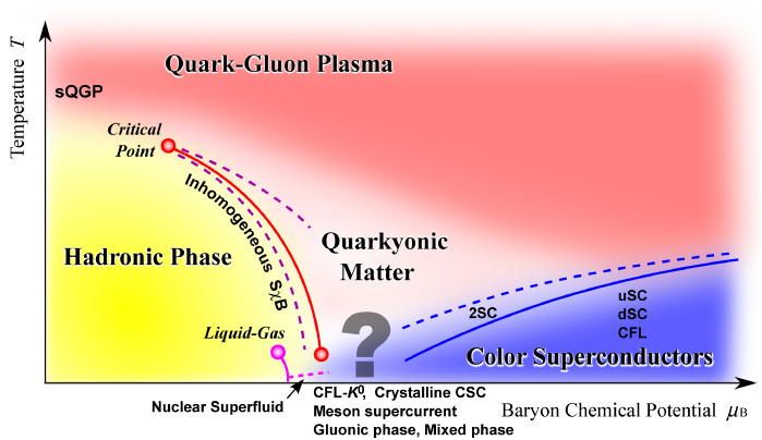
Figure 1: QCD phase diagram in the $\mu$-$T$ plane. Figure is taken from Ref. [1].

We can add more external parameters or axes to Fig. 1 to construct a multidimensional space. For example, instead of having a common quark chemical potential for all flavors, we can introduce a chemical potential $\mu_{f}$ for each of them. For $n_{f}=2$, we can therefore either use $\mu_{u}$ and $\mu_{d}$ or equivalently use baryon and isospin chemical potentials $\mu_{B}$ and $\mu_{I}$. The relations between the two sets of chemical potentials are $\mu_{u}=\mu+\mu_{I}$ and $\mu_{d}=\mu-\mu_{I}$ where $\mu={1\over 3}\mu_{B}$ is the quark chemical potential. A nonzero value of $\mu_{I}$ introduces an imbalance between the $u$ and the $d$-quarks, which gives rise to Bose-Einstein condensation of pions if it is large enough.

The phase diagram in the $\mu_{I}$-$T$ plane was conjectured in 2001 by Son and Stephanov [4], and a possible scenario is shown in Fig. 2. In the lower left corner, there is a hadronic phase. As one cranks up the temperatue, there is a deconfinement transition to a quark-gluon plasma phase. This transition is indicated by the dashed red line. Along the $\mu_{I}$-axis, one enters a Bose-condensed phase of pions. This phase breaks an $O(2)$ symmetry associated with the conservation of the third component of isospin. At $T=0$, the onset of charged pion condesation is exactly at $\mu_{I}={1\over 2}m_{\pi}$.  For larger values yet of $\mu_{I}$, there is a crossover transition to a BCS state.  In this phase, there is a condensate of weakly bound Cooper pairs, rather than a condensate of tightly bound charged pions. The blue line indicates the transition to a Bose-condensed phase (blue region) or a BCS state (green region).

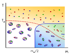
Figure 2: Phase diagram in the $\mu_{I}$-$T$ plane. Figure is taken from [11].

In this talk, I would like to discuss certain aspects of the QCD phase diagram, namely that of pion condensation at finite isospin density [2, 3]. Specifically, I want to address the following

1. Phase diagram in the $\mu$-$\mu_{I}$ plane at $T=0$. Inhomogeneous phases and competition with an inhomogeneous pion condensate

2. Phase diagram in the $\mu_{I}$-$T$ plane. Pion condensation, BEC-BCS transition, chiral and deconfinement transitions.

1 Quark-meson model

In order to map out the phase diagrams, we employ the quark-meson model as an effective low-energy model of QCD. The Minkowski Lagrangian including $\mu_{u}$ and $\mu_{d}$ reads

$${\cal L} = {1\over 2}\left[(\partial_{\mu}\sigma)(\partial^{\mu}\sigma)+(\partial_{\mu}\pi_{3})(\partial^{\mu}\pi_{3})\right]+(\partial_{\mu}+2i\mu_{I}\delta_{\mu}^{0})\pi^{+}(\partial^{\mu}-2i\mu_{I}\delta_{0}^{\mu})\pi^{-}-{1\over 2}m^{2}(\sigma^{2}+\pi_{3}^{2}$$ (1)

$$+2\pi^{+}\pi^{-})-{\lambda\over 24}(\sigma^{2}+\pi_{3}^{2}+2\pi^{+}\pi^{-})^{2}+h\sigma+\bar{\psi}\left[i/\!\!\!\!\partial+\mu_{f}\gamma^{0}-g(\sigma+i\gamma^{5}{\bm{\tau}}\cdot{\bm{\pi}})\right]\psi\;.$$

We will in the following allow for an inhomogeneous chiral condensate, several different ansätze have been discussed in the literature, for example a chiral-density wave (CDW) and a chiral soliton lattice.We choose the simplest ansatz, namely that of a CDW,

$$\sigma=\phi_{0}\cos(qz)\;,\hskip 14.22636pt\pi_{1}=\pi_{0}\;,\hskip 14.22636pt\pi_{2}=0\;,\hskip 14.22636pt\pi_{3}=\phi_{0}\sin(qz)\;,$$

where $\phi_{0}$ is the magnitude of the chiral condesate, $q$ is a wavevector, and $\pi_{0}$ is a homogeneous pion condensate. Below we will express the effective potential using the variables $\Delta=g\phi_{0}$ and $\rho=g\pi_{0}$.

There are two technical details I would like to briefly mention, namely that of parameter fixing and regulator artefacts. In mean-field calculations it is common to determine the parameters of the Lagrangian at tree level. However, this is inconsistent. One must determine the parameters to the same accuracy as one is calculating the effective potential. We are calculating the effective potential to one loop in the large-$N_{c}$ limit, which means that we integrate over the fermions, but treat the mesons at tree level. Consequently, we must determine the parameters in Eq. (1) in the same approximation. If one determines the parameters at tree level and the effective potential in the one-loop large-$N_{c}$ approximation, the onset of BEC will not be at $\mu_{I}={1\over 2}m_{\pi}$, in fact in some case there are substantial deviations from this exact result. This point has been ignored in most calculations to date. Secondly, in calculations using the NJL model, one is typically using a hard momentum cutoff. In cases with inhomogeneous phases, this leads to an asymmetry in the states included due to the sign of $q$ in the different quark dispersion relations. This leads to a $q$-dependent effective potential even in the limit $\Delta\rightarrow 0$. This is inconsistent and one must typically subtract a $q$-dependent term to remedy this. In the present calculations in the QM model, we are using dimensional regularization. We have explicitly checked that the effective potential is consistent, i.e. it is independent of the wavevector $q$ in the limit $\Delta\rightarrow 0$.

Let us return to the QM Lagrangian (1). The quark energies are

$$E_{u}^{\pm} = E(\pm q,-\mu_{I})\;,\hskip 14.22636ptE_{d}^{\pm}=E(\pm q,\mu_{I})\;,\hskip 14.22636ptE_{\bar{u}}^{\pm}=E(\pm q,\mu_{I})\;,\hskip 14.22636ptE_{\bar{d}}^{\pm}=E(\pm q,-\mu_{I})\;,$$

where

$$E(q,\mu_{I}) = \left[\left(\sqrt{p_{\perp}^{2}+\left(\sqrt{p_{\parallel}^{2}+\Delta^{2}}+{q\over 2}\right)^{2}}+{\mu_{I}}\right)^{2}+\rho^{2}\right]^{1\over 2}\;.$$ (2)

Note in particular that the quark energies depend on the isospin chemical potential. After regularization and renormalization, the zero-temperature part of the effective potential can be expressed in terms of the physical meson masses and the pion-decay constant as 

$$V_{\rm 1-loop} = {1\over 2}f_{\pi}^{2}q^{2}\left\{1-\dfrac{4m_{q}^{2}N_{c}}{(4\pi)^{2}f_{\pi}^{2}}\left[\log\mbox{$\Delta^{2}+\rho^{2}\over m_{q}^{2}$}+F(m_{\pi}^{2})+m_{\pi}^{2}F^{\prime}(m_{\pi}^{2})\right]\right\}{\Delta^{2}\over m_{q}^{2}}$$ (3)

$$+\dfrac{3}{4}m_{\pi}^{2}f_{\pi}^{2}\left\{1-\dfrac{4m_{q}^{2}N_{c}}{(4\pi)^{2}f_{\pi}^{2}}m_{\pi}^{2}F^{\prime}(m_{\pi}^{2})\right\}\dfrac{\Delta^{2}+\rho^{2}}{m_{q}^{2}}$$

$$-\dfrac{1}{4}m_{\sigma}^{2}f_{\pi}^{2}\left\{1+\dfrac{4m_{q}^{2}N_{c}}{(4\pi)^{2}f_{\pi}^{2}}\left[\left(1-\mbox{$4m_{q}^{2}\over m_{\sigma}^{2}$}\right)F(m_{\sigma}^{2})+\dfrac{4m_{q}^{2}}{m_{\sigma}^{2}}-F(m_{\pi}^{2})-m_{\pi}^{2}F^{\prime}(m_{\pi}^{2})\right]\right\}\dfrac{\Delta^{2}+\rho^{2}}{m_{q}^{2}}$$

$$-2\mu_{I}^{2}f_{\pi}^{2}\left\{1-\dfrac{4m_{q}^{2}N_{c}}{(4\pi)^{2}f_{\pi}^{2}}\left[\log\mbox{$\Delta^{2}+\rho^{2}\over m_{q}^{2}$}+F(m_{\pi}^{2})+m_{\pi}^{2}F^{\prime}(m_{\pi}^{2})\right]\right\}{\rho^{2}\over m_{q}^{2}}$$

$$+\dfrac{1}{8}m_{\sigma}^{2}f_{\pi}^{2}\Bigg{\{}1-\dfrac{4m_{q}^{2}N_{c}}{(4\pi)^{2}f_{\pi}^{2}}\Bigg{[}\dfrac{4m_{q}^{2}}{m_{\sigma}^{2}}\left(\log\mbox{$\Delta^{2}+\rho^{2}\over m_{q}^{2}$}-\mbox{$3\over 2$}\right)-\left(1-\mbox{$4m_{q}^{2}\over m_{\sigma}^{2}$}\right)F(m_{\sigma}^{2})$$

$$+F(m_{\pi}^{2})+m_{\pi}^{2}F^{\prime}(m_{\pi}^{2})\Bigg{]}\Bigg{\}}\dfrac{(\Delta^{2}+\rho^{2})^{2}}{m_{q}^{4}}-\dfrac{1}{8}m_{\pi}^{2}f_{\pi}^{2}\left[1-\dfrac{4m_{q}^{2}N_{c}}{(4\pi)^{2}f_{\pi}^{2}}m_{\pi}^{2}F^{\prime}(m_{\pi}^{2})\right]\dfrac{(\Delta^{2}+\rho^{2})^{2}}{m_{q}^{4}}$$

$$-m_{\pi}^{2}f_{\pi}^{2}\left[1-\dfrac{4m_{q}^{2}N_{c}}{(4\pi)^{2}f_{\pi}^{2}}m_{\pi}^{2}F^{\prime}(m_{\pi}^{2})\right]\dfrac{\Delta}{m_{q}}\delta_{q,0}+V_{\rm fin}\;,$$

where $V_{\rm fin}$ is a finite term that must be evaluated numerically. The linear term is responsible for explicit chiral symmetry breaking. It only contributes when $q=0$, i.e. in the homogeneous case; for nonzero $q$ this term averages to zero over a sufficiently large spatial volume of the system. The finite-temperature part of the one-loop effective potential is

$$V_{T} = -2N_{c}T\int_{p}\bigg{\{}\log\Big{[}1+e^{-\beta(E_{u}-\mu)}\Big{]}+\log\Big{[}1+e^{-\beta(E_{\bar{u}}+\mu)}\Big{]}\bigg{\}}+{u\leftrightarrow d}\;.$$ (4)

2 Coupling to the Polyakov loop

The Wilson line which wraps all the way around in imaginary time is defined as

$$L({\bf x}) = {\cal P}\exp\left[i\int_{0}^{\beta}d\tau A_{4}({\bf x},\tau)\right]\;,$$ (5)

where ${\cal P}$ is time ordering. The Wilson line is not gauge invariant, but taking the trace of it gives a gauge-invariant object, namely the Polyakov loop ${\rm Tr}\,L$. The Polyakov loop is, however, not invariant under the socalled center symmetry of the (pure glue) QCD Lagrangian, but transforms as ${\rm Tr}\,L\rightarrow e^{i{n\over N_{c}}}{\rm Tr}\,L$, where $n=0,1,2...N_{c}-1$ and $e^{i{n\over N_{c}}}$ is one of the $N_{c}$ roots of unity. A nonzero expectation value of the Polyakov loop therefore signals the breaking of the center symmetry. The expectation value of the correlator of Polyakov loop and its conjugate is related to the free energy of a quark and an antiquark. Employing cluster decomposition, the expectation value of the Polyakov loop itself is related to the free energy of a single quark; A vanishing value of ${\rm Tr}\,L$ corresponds to an infinite free energy of a single quark and a vanishing value of ${\rm Tr}\,L^{\dagger}$ corresponds to an infinite free energy of an antiquark, and therefore signals confinement. If we denote by $\Phi$ the expectation value of ${\rm Tr}\,L$ and $\bar{\Phi}$ of ${\rm Tr}\,L^{\dagger}$, the medium contribution reads

$$V_{T} = -2T\int{d^{3}p\over(2\pi)^{3}}\bigg{\{}{\rm Tr}\log\Big{[}1+3(\Phi+\bar{\Phi}e^{-\beta(E_{u}-\mu)})e^{-\beta(E_{u}-\mu)}+e^{-3\beta(E_{u}-\mu)}\Big{]}$$ (6)

$$+{\rm Tr}\log\Big{[}1+3(\bar{\Phi}+\Phi e^{-\beta(E_{\bar{u}}+\mu)})e^{-\beta(E_{\bar{u}}+\mu)}+e^{-3\beta(E_{\bar{u}}+\mu)}\Big{]}\bigg{\}}+{u\leftrightarrow d}\;.$$

We note that the symmetry between $\Phi$ and $\bar{\Phi}$ implies $\Phi=\bar{\Phi}$. The expression for $V_{T}$ is also manifestly real, reflecting that there is no sign problem at finite $\mu_{I}$ and zero $\mu_{B}$. Finally, for $\Phi=\bar{\Phi}=1$, we recover the standard expression for the fermionic contribution (4) for $N_{c}=3$.

We also need to introduce a potential ${\cal U}$ from the glue sector. The terms are constructed from $\Phi$ and $\bar{\Phi}$ such that it satisfies the symmetries. There are several such potentials on the market. We choose the following logarithmic potential [5]

$${{\cal U}\over{T^{4}}} = -{1\over 2}a\Phi\bar{\Phi}+b\log\left[1-6\Phi\bar{\Phi}+4(\Phi^{3}+\bar{\Phi}^{3})-3(\Phi\bar{\Phi})^{2}\right]\;,$$ (7)

with $a=3.51-2.47\left({T_{0}\over T}\right)+15.2\left({T_{0}\over T}\right)^{2}$ and $b=-1.75\left({T_{0}\over T}\right)^{3}$ . The parameters are determined such that the potential reproduces the pressure for pure-glue QCD as calculated on the lattice for temperatures around the critical temperature. Since the critical temperature depends on the number of flavors $n_{f}$ and $\mu_{I}$, one can refine the potential by making $T_{0}$ dependent on these parameters, $T_{0}(N_{f},\mu_{I})=T_{\tau}e^{-1/(\alpha_{0}b(\mu_{I}))}$ with $b(\mu_{I})={1\over 6\pi}(11N_{c}-2N_{f})-b_{\mu_{I}}{\mu_{I}^{2}\over T_{\tau}^{2}}$ and $T_{\tau}=1.77\;\text{GeV}$ and $\alpha_{0}=0.304$ are determined such that the transition temperature for pure glue at $\mu_{I}=0$ is $T_{0}=270$ MeV [6]. In the numerical work, we use $m_{\pi}=140$ MeV, $m_{\sigma}=500$ MeV, $\Delta=300$ MeV, and $f_{\pi}=93$ MeV.

3 Phase diagram in the $\mu$-$\mu_{I}$ plane

We first discuss the results for the phase diagram in the $\mu$-$\mu_{I}$ plane at $T=0$ in the chiral limit, which is shown in the left panel of Fig. 3. Dashed lines indicate first-order transitions while solid lines indicate second-order transitions. The black dot indicates the endpoint of the first-order line. The vacuum phase is part of the $\mu$-axis (recall that in the chiral limit, the onset of pion condensation is at $\mu_{I}=0$), ranging from $\mu=0$ to $\mu=300$ MeV. In this phase all the thermodynamic functions are independent of the quark chemical potentials. In the region to the left of the blue line, there is a nonzero pion condensate which is independent of $\mu$. In the wedge-like shaped region between the blue and green lines, there is a phase with a $\mu$-dependent pion condensate and a vanishing chiral condensate. In this phase the isospin and quark densities are nonzero. In the region between the green and red lines, we have an inhomogeneous phase with a nonzero wavevector $q$. In this phase, the pion condensate is zero; thus there is no coexistence of an inhomogeneous chiral condensate and a homogeneous pion condensate. Finally, the region to the right of red, blue, and green line segments is the symmetric phase, where $\Delta=\rho=q=0$. The blue dot marks the Lifshitz point where the homogeneous, inhomogeneous and chi- rally symmetric phases connect. In the right panel of Fig. 3, we show the pion condensate $\rho$ (green line), the magnitude of the chiral condensate $\Delta$ (blue line), and the wavevector $q$ (red line) as functions of $\mu$ for fixed $\mu_{I}=5$ MeV. This corresponds to a horizontal line in the phase diagram.

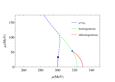
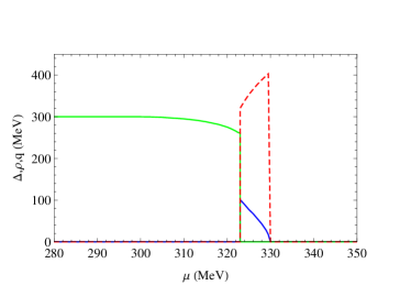
Figure 3: Phase diagram in the chiral limit (left) and $\rho$, $\Delta$, and $q$ as functions of $\mu$ for $\mu_{I}=5$ MeV (right). See main text for details.

In the left panel of Fig. 4, we show the window of inhomogeneous chiral condensate for $\mu_{I}=0$, i.e. on the $\mu$-axis as a function of the pion mass. The inhomogeneous phase ceases to exist for pion masses larger than $37.1$ MeV and so is not present at the physical point This is contrast to the QM study in Ref. [7] where an inhomogeneous phase is found at the physical point. However, in that paper the parameters were determined at tree level, which may explain the difference with the results presented here. The question of inhomogeneous phases in QCD was also addressed by Buballa at this meeting using the NJL model, in particular discussing the role of the quark masses [8]. Performing a Ginzburg-Landau analysis, they find an inhomogeneous phase which shrinks with increasing quark mass, but survives at the physical point.

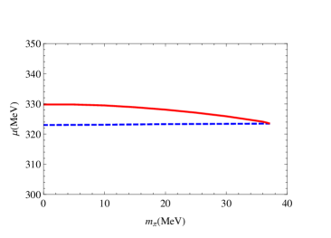
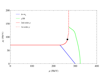
Figure 4: Window of inhomogeneous phase as a function of the pion mass for $\mu_{I}=0$ (left) and the homogeneous phase diagram at the physical point (right).

In the right panel of Fig. 4, we show the phase diagram at the physical point. The thermodynamic observables are independent of $\mu$ and $\mu_{I}$ in the region bounded by the $\mu_{I}$ and $\mu$ axes, and the straight lines given by $\mu+\mu_{I}=gf_{\pi}=m_{q}$ (blue line) and $\mu_{I}=\mu_{i}^{c}={1\over 2}m_{\pi}$ (red line). We therefore refer to this as the vacuum phase. The red line shows the phase boundary between a phase with $\rho=0$ and a pion-condensed phase. The transition is second order when the red line is solid and first order when it is dashed. The solid dot indicates the position of the critical end point where the first-order line ends, and is located at $(\mu,\mu_{I})=(264,91)$ MeV. The green line indicates the boundary between a chirally broken phase and a phase where chiral symmetry is approximately restored. This line is defined by the inflection point of the chiral condensate in the $\mu$-direction. The region bounded by the three lines is a phase with chiral symmetry breaking but no pion condensate. The effective potential depends on $\mu$ and $\mu_{I}$ and therefore the quark and isospin densities are nonzero.

4 Phase diagram in the $\mu_{I}$-$T$ plane

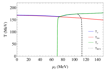
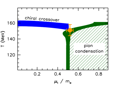
Figure 5: Phase diagram in the $\mu_{I}$-$T$ plane from the PQM model (left) and from the lattice simulations of Refs. [9, 10, 11].

In the left panel of Fig. 5, we show the phase diagram in the $\mu_{I}$-$T$ diagram resulting from our PQM model calculation. The green line indicates the transition to a pion-condensed phase, where the $O(2)$-symmetry associated with the conservation of the third component of the isospin is broken. This transition is second order everywhere. At $T=0$ this transition takes place at $\mu_{I}={1\over 2}m_{\pi}$ by construction. The chiral transition line is in blue, while the transition line for the deconfinement transition is in red. In the noncondensed phase, these coincide. When these lines meet the BEC line, they depart and the former coincides the BEC line. The transition line for deconfinement penetrates into condensed phase. Finally, the dashed line indicates the BEC-BCS crossover defined by the condition $\Delta>\mu_{I}$, i.e. when the dispersion relations for the $u$-quark and $\bar{d}$-quark no longer have their minima at $p=0$, but rather at $p=\sqrt{\Delta^{2}-\mu_{I}^{2}}$. In the right panel of Fig. 5, we see the lattice results of Refs. [9, 10, 11]. The blue band indicates the chiral crossover. Within the uncertainty it coincides with the deconfinement transition. The green band indicates the second-order transition to a Bose-Einstein condensed state. The three transition meet at the yellow point. Their simulations also indicate that the deconfinement transition temperature decreases and the transition line smoothly penetrates into the pion-condensed phase.

5 Summary

I would like to finish this talk by highlighting our main results and the comparison with lattice results from Refs. [9, 10, 11].

1. Rich phase diagrams. Inhomogeneous chiral condensate excluded for $m_{\pi}>37.1$ MeV.

2. No inhomogeneous chiral condensate coexists with a homogeneous pion condensate.

3. Good agreement between lattice simulations and model calculations:

   1. Second-order transition to a BEC state, which is in the $O(2)$ universality class. At $T=0$, onset of pion condensation at exactly $\mu_{I}^{c}={1\over 2}m_{\pi}$.

   2. BEC and chiral transition lines merge at large $\mu_{I}$.

   3. The deconfinement transition smoothly penetrates into the BEC phase.

References

- [1] K. Fukushima and T. Hatsuda, Rept. Prog. Phys. 74,014001 (2011).
- [2] J. O. Andersen and P. Kneschke, Phys. Rev. D 97, 076005 (2018).
- [3] P. Adhikari, Jens O. Andersen, and P. Kneschke, e-Print: arXiv:1805.08599.
- [4] D. T. Son and M. Stephanov, Phys. Rev. Lett. 88, 202302 (2002).
- [5] S. Roessner, C. Ratti and W. Weise, Phys. Rev. D 75, 034007 (2007).
- [6] B.-J. Schaefer, J. M. Pawlowski, and J. Wambach, Phys. Rev. D 76, 074023 (2007).
- [7] D. Nickel, Phys. Rev. D 80, 074025 (2009).
- [8] M. Buballa, these proceedings; M. Buballa and S, Carignano e-Print: arXiv:1809.10066.
- [9] B. B. Brandt and G. Endrődi, PoS LATTICE 2016, 039 (2016).
- [10] B. B. Brandt, G. Endrődi, and S. Schmalzbauer, EPJ Web Conf. 175, 07020 (2018).
- [11] B. B. Brandt, G. Endrődi, and S. Schmalzbauer, Phys. Rev. D 97, 054514 (2018).
- [12] K. Kamikado, N. Strodthoff, L. von Smekal, and J. Wambach, Phys. Lett. B 718, 1044 (2013).