PLL and Costas loop based carrier recovery circuits for 4QAM: non-linear analysis and simulation

Abstract

Design of stable carrier recovery circuits are used in many applications: wireless digital communication, optical communication, microwave devices and other applications. Quadrature Phase-Shift Keying (QPSK, 4-QAM) is used as modulation technique in many of these applications, since QPSK provides double the data rate of classic Binary PSK (BPSK) modulation. Analysis of Costas loop is a hard task because of its non-linearity. In this work we consider two well-known modifications of 4QAM Costas loop circuits and discuss a new circuit proposed by J. Ladvanszky. MATLAB Simulink models of the circuits are provided and the noise analysis is performed.

1 Introduction

Nowadays phase-locked loop based circuits are widely used in various intelligent systems for synchronization and communication [1, 2, 3]. Phase-shift keying (PSK) is a digital modulation process which conveys data by changing (modulating) the phase of a reference signal (the carrier wave). The modulation occurs by varying the phase of sine and cosine inputs at a precise time. It is widely used for wireless networks (WiFi), radio-frequency identification (RFID), and Bluetooth communication. First widely adopted circuit for demodulation of Binary PSK signals (BPSK) was invented by famous engineer John P. Costas [4]. Later it was adopted for more efficient modulation technique — quadrature phase-shift keying (also called QPSK, 4-PSK and 4-QAM) [5, 6]. With four phases, QPSK can encode two bits per symbol, while BPSK can encode only one bit per symbol. More sophisticated modulation techniques (8-QAM, 16-QAM and higher) require transmission with high signal-to-noise ratio. One of the main characteristics of Costas loops is the lock-in range (introduced in [7],[8, p.70]). Here we follow the rigorous mathematical definition of lock-in range for PLL-based circuits suggested in [9, 10, 5].

In this work we study various models of QPSK Costas loop including a new model based on the folding operation (corresponding consideration of BPSK Costas loop can be found, e.g. in [11, 12, 13, 5, 14]). Often only linear analysis and straight-forward circuit simulation is used to study lock-in range, which may lead to misleading conclusions. In this work non-linear mathematical models for each circuits are developed and the lock-in ranges for these models are computed. Finally, we compare noise characteristics of considered circuits (see, e.g. [15]).

1.1 Classical QPSK Costas loop

Consider the classical QPSK Costas loop operation (see Fig. 1).

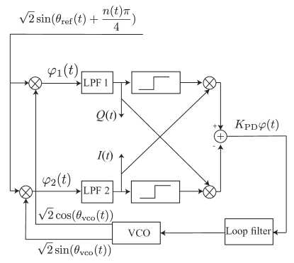
Figure 1: QPSK Costas loop operation.

It is convenient to consider input QPSK signal in the following form

$$\sqrt{2}\sin(\theta_{\rm ref}(t)+\tfrac{n(t)\pi}{4}),\quad\theta_{\rm ref}(t)=\omega_{\rm ref}t,\ \ n(t)\in\{1,3,5,7\}.$$

Here $\dot{\theta}_{\rm ref}(t)=\omega_{\rm ref}$ denotes carrier frequency and $n(t)$ corresponds to digital data (two bits per symbol). The input signal is multiplied by inphase and quadrature phase VCO outputs $\sqrt{2}\cos(\theta_{\rm vco}(t))$ and $\sqrt{2}\sin(\theta_{\rm vco}(t))$, with $\theta_{\rm vco}(t)$ being the phase of VCO. The resulting signals are

$$\varphi_{1}(t)=2\cos(\theta_{\rm vco}(t))\sin(\theta_{\rm ref}(t)+\tfrac{n(t)\pi}{4})=$$

$$=\sin(\theta_{\rm ref}(t)+\tfrac{n(t)\pi}{4}-\theta_{\rm vco}(t))+$$

$$\qquad+\sin(\theta_{\rm ref}(t)+\tfrac{n(t)\pi}{4}+\theta_{\rm vco}(t)),$$

$$\varphi_{2}(t)=2\sin(\theta_{\rm vco}(t))\sin(\theta_{\rm ref}(t)+\tfrac{n(t)\pi}{4})=$$

$$=\cos(\theta_{\rm ref}(t)+\tfrac{n(t)\pi}{4}-\theta_{\rm vco}(t))-$$

$$\qquad-\cos(\theta_{\rm ref}(t)+\tfrac{n(t)\pi}{4}+\theta_{\rm vco}(t))$$

Here, from an engineering point of view, the high-frequency terms $\cos(\theta_{\rm ref}(t)+\theta_{\rm vco}(t)+\tfrac{n(t)\pi}{4})$ and $\sin(\theta_{\rm ref}(t)+\theta_{\rm vco}(t)+\tfrac{n(t)\pi}{4})$ are removed by low-pass filters LPF 1 and LPF 2. Thus, the signals $Q(t)$ and $I(t)$ on the upper and lower branches can be approximated as

$$Q(t)\approx\sin(\theta_{e}(t)+\tfrac{n(t)\pi}{4}),$$ (1)

$$I(t)\approx\cos(\theta_{e}(t)+\tfrac{n(t)\pi}{4}),$$

$$\theta_{e}(t)=\theta_{\rm ref}(t)-\theta_{\rm vco}(t).$$

Signals $I(t)$ and $Q(t)$ are used for demodulation, i.e. decoding $n(t)$. In the case of complete synchronization of VCO to the carrier, i.e. $\theta_{e}(t)=0$, one can determine $n(t)$ from signs of $I(t)$ and $Q(t)$ using the following table:

	$I>0$	$I<0$
$Q>0$	$n=1$	$n=3$
$Q<0$	$n=7$	$n=5$

After the filtration, both signals $\varphi_{1}(t)$ and $\varphi_{2}(t)$ pass through the limiters. Then the outputs of the limiters $\mbox{sign\,}\big{(}Q(t)\big{)}$ and $\mbox{sign\,}\big{(}I(t)\big{)}$ are multiplied by $I(t)$ and $Q(t)$. Using (1) we get (see, e.g. [5])

$$K_{\rm PD}\varphi(t)=I(t)\mbox{sign\,}\big{(}Q(t)\big{)}-Q(t)\mbox{sign\,}\big{(}I(t)\big{)}$$ (2)

$$=\cos(\theta_{e}(t)+\tfrac{n(t)\pi}{4})\mbox{sign\,}(\sin(\theta_{e}(t)+\tfrac{n(t)\pi}{4}))-$$

$$-\sin(\theta_{e}(t)+\tfrac{n(t)\pi}{4})\mbox{sign\,}(\cos(\theta_{e}(t)+\tfrac{n(t)\pi}{4}))$$

$$=\,K_{\rm PD}\varphi(\theta_{e}(t))\,=\,\left\{\begin{array}[]{ll}-\frac{1}{\sqrt{2}}\sin(\theta_{e}(t)),&-\frac{\pi}{4}<\theta_{e}(t)<\frac{\pi}{4},\\ \frac{1}{\sqrt{2}}\cos(\theta_{e}(t)),&\frac{\pi}{4}<\theta_{e}(t)<\frac{3\pi}{4},\\ \frac{1}{\sqrt{2}}\sin(\theta_{e}(t)),&\frac{3\pi}{4}<\theta_{e}(t)<\frac{5\pi}{4},\\ -\frac{1}{\sqrt{2}}\cos(\theta_{e}(t)),&\frac{5\pi}{4}<\theta_{e}(t)<-\frac{\pi}{4}.\\ \end{array}\right.$$

Here $K_{\rm PD}=\frac{1}{2}$, $\varphi(\theta_{e}(t))$ is a piecewise-smooth $\frac{\pi}{2}$—periodic function (see Fig. 2) with unit amplitude.

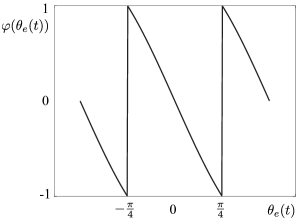
Figure 2: Phase detector characteristic of QPSK Costas loop $\varphi(\theta_{e})$.

The periodicity of function $\varphi(\theta_{e})$ makes the loop filter input $\varphi(t)$ insensitive to change of the data signal $n(t)$. The resulting signal $\varphi(t)$ after the filtration by the loop filter forms the control signal $g(t)$ for the VCO.

The relation between the input $\varphi(t)$ and the output $g(t)$ of the Loop filter has the form

$$\frac{dx}{dt}=Ax+bK_{\rm PD}\varphi(t),\ g(t)=c^{*}x+hK_{\rm PD}\varphi(t).$$ (3)

Here $A$ is a constant matrix, vector $x(t)$ is a filter state, $b,c$ are constant vectors. Corresponding transfer function takes the form

$$H(s)=-c^{*}(A-sI)^{-1}b+h.$$ (4)

The control signal $g(t)$ is used to adjust VCO frequency to the frequency of input carrier signal

$$\dot{\theta}_{\rm vco}(t)=\omega_{\rm vco}(t)=\omega_{\rm vco}^{\text{free}}+K_{\rm vco}g(t).$$ (5)

Here $\omega_{\rm vco}^{\text{free}}$ is free-running frequency of VCO and $K_{\rm vco}$ is VCO gain.

For the constant frequency of input carrier

$$\dot{\theta}_{\rm ref}(t)=\omega_{\rm ref}(t)\equiv\omega_{\rm ref},$$ (6)

equations (2)-(5) give the following mathematical model of Costas loop

$$\frac{dx}{dt}=Ax+bK_{\rm PD}\varphi(\theta_{e}),$$ (7)

$$\dot{\theta}_{e}=\omega_{\rm ref}-\omega_{\rm vco}^{\rm free}-K_{\rm vco}\Big{(}c^{*}x+hK_{\rm PD}\varphi(\theta_{e})\Big{)}.$$

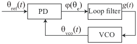
Figure 3: Classical mathematical model of QPSK Costas loop.

Non-linear mathematical model (7) and corresponding Fig. 3 is called the signal’s phase space model [10]. Engineers use this model for the approximate analysis of the circuit (see, e.g. [6]). Using the above signal’s phase space model, further we estimate the lock-in ranges for the considered QPSK circuits.

1.2 Fourth-power Costas loop

Consider variation of QPSK Costas loop shown in Fig. 4 (see, e.g. [19, 20], and for optical implementations [21]).

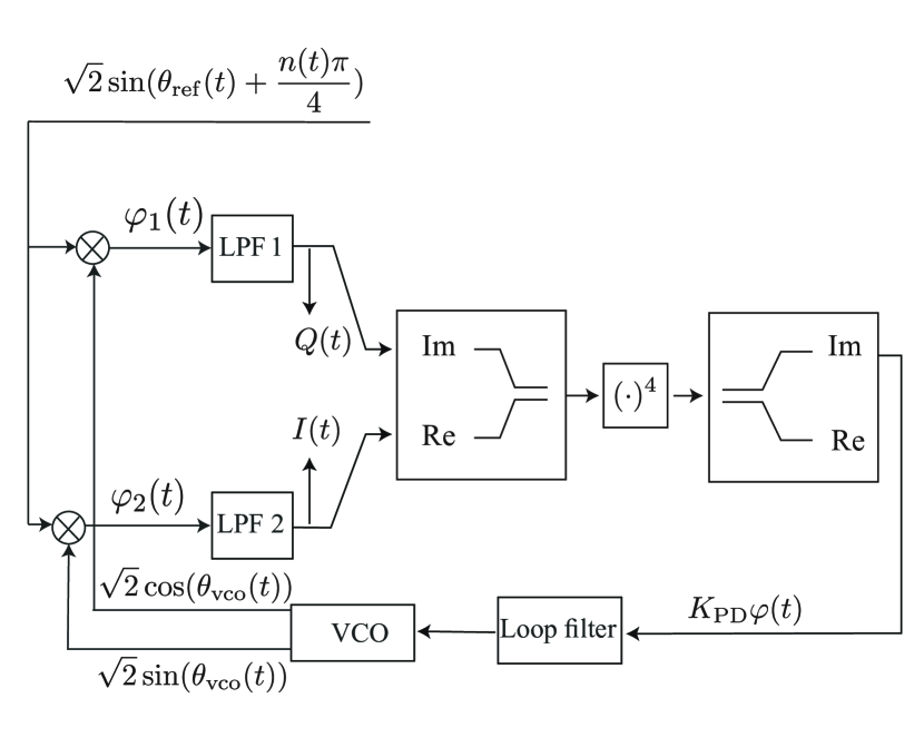
Figure 4: QPSK Costas loop with $(\cdot)^{4}$ block.

Similar to classic QPSK Costas loop (Fig. 1), input QPSK signal is multiplied by two outputs of VCO on each branch and outputs of multipliers filtered by corresponding low-pass filters. Then signals from two branches ($I(t)$ and $Q(t)$) are combined by Re Im block to complex signal, which is raised to the fourth power, and resulting signal is connected to input of VCO. Using apporximation (1), input of the loop filter can be approximated as follows

$$\varphi(\theta_{e}(t))=\text{Re}(\left(I(t)+jQ(t)\right)^{4}\approx-\sin(4\theta_{e}(t))$$ (8)

Here phase detector characteristic $\varphi(\theta_{e})=-\sin(4\theta_{e})$ is of unit amplitude. Therefore we get the following equation

$$\dot{x}=Ax-b\sin(4\theta_{e}),$$ (9)

$$\dot{\theta}_{e}=\omega_{e}^{\rm free}-K_{\rm vco}c^{*}x+K_{\rm vco}h\sin(4\theta_{e}).$$

1.3 Folding QPSK Costas loop

Now lets consider QPSK Costas loop proposed by János Ladvánszky [22] (see Fig. 5).

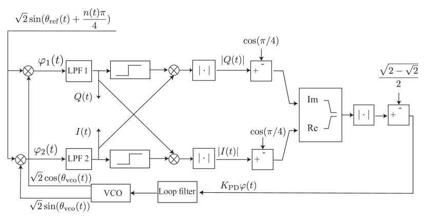
Figure 5: QPSK Costas loop with folding block.

Here input signal, VCO output, multipliers and filters (LPF 1, LPF 2, Loop filter) are the same as for classic QPSK Costas loop. As mentioned before, here we assume that low-pass filters completely eliminate the high-frequency oscillations. Using the assumption of low-pass filtration, this scheme can be simplified, see Fig. 6).

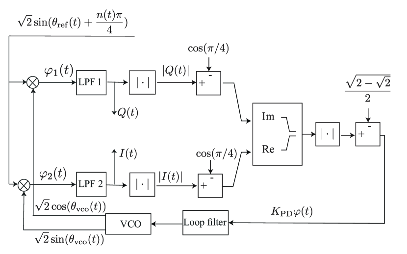
Figure 6: Simplified QPSK Costas loop with folding block.

These two block-schemes are equivalent because blocks which take absolute values have the same outputs:

$$|\sin(\theta_{e}(t)+\frac{n(t)\pi}{4})\mbox{sign\,}\cos(\theta_{e}(t)+\frac{n(t)\pi}{4})|=$$ (10)

$$=|\sin(\theta_{e}(t)+\frac{n(t)\pi}{4})|=|Q(t)|,$$

$$|\cos(\theta_{e}(t)+\frac{n(t)\pi}{4})\mbox{sign\,}\sin(\theta_{e}(t)+\frac{n(t)\pi}{4})|=$$

$$=|\cos(\theta_{e}(t)+\frac{n(t)\pi}{4})|=|I(t)|,$$

These signals are shifted by $-\cos(\frac{\pi}{4})$ and combined by Re Im block to complex signal

$$|\cos(\theta_{e}(t)+\tfrac{\pi}{4})|-\cos(\tfrac{\pi}{4})+j(|\sin(\theta_{e}(t)+\tfrac{\pi}{4})|-\sin(\tfrac{\pi}{4})).$$ (11)

Then absolute value of complex signal is centered, and after filtration by Loop filter used as control signal for VCO:

$$K_{\rm PD}\varphi(\theta_{e}(t))=\big{|}|\cos(\theta_{e}(t)+\tfrac{\pi}{4})|-\cos(\tfrac{\pi}{4})+$$ (12)

$$+j(|\sin(\theta_{e}(t)+\tfrac{\pi}{4})|-\sin(\tfrac{\pi}{4}))\big{|}-\frac{\sqrt{2-\sqrt{2}}}{2}=$$

$$\sqrt{2-\sqrt{2}(|\sin(\theta_{e}(t)+\tfrac{\pi}{4})|+|\cos(\theta_{e}(t)+\tfrac{\pi}{4})|)}-\frac{\sqrt{2-\sqrt{2}}}{2}.$$

Here amplitude of (12) is $K_{\rm pd}=\frac{\sqrt{2-\sqrt{2}}}{2}$ and $\varphi(\theta_{e})$ is normalized phase detector characteristic with unit amplitude.

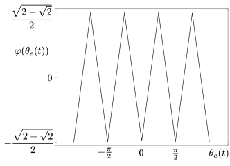
Figure 7: Phase detector characteristic for the folding QPSK Costas loop

Note, that the folding version can work for higher order constellations as well, however, the 4th power version can work only for 4QAM.

2 Hold-in and lock-in ranges

Since block-scheme on Fig. 3 and corresponding equations (7) describe classical analog PLL, it is possible to apply the same analysis to QPSK Costas loops. For proportionally-integrating loop filter the hold-in and pull-in ranges are infinite [10]. The lock-in range can be recalculated from the lock-in range for the PLL with corresponding phase detector characteristics.

Since PLL system (7) is $2\pi$-periodic (while for QPSK Costas it is $\frac{\pi}{2}$-periodic), in order to transfer results to QPSK Costas loops it is necessary to consider change of variables $\tilde{\theta}_{e}=4\theta_{e}$, $\tilde{\omega}_{e}=\frac{\omega_{\rm ref}-\omega_{\rm vco}^{\rm free}}{4}$, $\tilde{v}_{e}(\tilde{\theta}_{e})=\varphi(\theta_{e})$. After the change of variables we get

$$\frac{dx}{dt}=Ax-b\tilde{v}(\tilde{\theta}_{e}),$$ (13)

$$\dot{\tilde{\theta_{e}}}=4\omega_{\rm ref}-4\omega_{\rm vco}^{\rm free}-4K_{\rm vco}\Big{(}c^{*}x-h\tilde{v}(\tilde{\theta}_{e})\Big{)}.$$

For sinusoidal characteristics (in the case of 4th power QPSK and two-phase Costas suggested by Roland Best [5]) $\varphi(\theta_{e})=-\sin(4\theta_{e})$ equations (13) take the following form

$$\frac{dx}{dt}=Ax-b\sin(\tilde{\theta}_{e}),$$ (14)

$$\dot{\tilde{\theta_{e}}}=4\omega_{\rm ref}-4\omega_{\rm vco}^{\rm free}-4K_{\rm vco}\Big{(}c^{*}x-h\sin(\tilde{\theta}_{e})\Big{)}.$$

Lock-in range for PLL-based circuits which are described by (14) is computed numerically and given in [23]. For classical loop the phase-detector characteristic is almost sawtooth (maximum deviation is less than $0.05$, see Fig. 8).

Figure 8: Normalized PD characteristic of the classic QPSK Costas loop and sawtooth characteristic

For folding loop PD characteristics is almost triangular (maximum deviation is less than $0.03$, see Fig. 9).

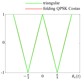
Figure 9: Normalized PD characteristic of folding QPSK Costas and triangular characteristic

Therefore we can use estimates of the lock-in range of classic PLL with corresponding PD characteristics [10, 24, 25].

2.1 Classical QPSK Costas

$$\omega_{l}=2\frac{a\sqrt{\pi}}{\tau_{2}}\hskip 2.84544pt\operatorname{exp}\left(\displaystyle\frac{a}{2d_{-}}\ln\left(\frac{d_{+}+d_{-}}{d_{+}-d_{-}}\right)\right);$$ (15)

$$\text{ where }a=\displaystyle\sqrt{\frac{4K_{\rm vco}\tau_{2}^{2}}{\tau_{1}}},\hskip 14.22636ptd_{-}=|a|,\hskip 14.22636ptd_{+}=\sqrt{a^{2}+4\pi}.$$

2.2 4th power QPSK Costas

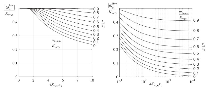
Figure 10: Lock-in range for 4th power QPSK Costas loop

2.3 Folding QPSK Costas

$$\textit{(i)}\text{ if }a^{2}-2\pi>0,$$

$$\quad\text{ then }\omega_{l}=2\frac{a\sqrt{\pi}}{\tau_{2}}\hskip 2.84544pt\operatorname{exp}\left(\frac{a}{2d_{-}}\ln\left(\frac{d_{+}+d_{-}}{d_{+}-d_{-}}\right)\right);$$

$$\textit{(ii)}\text{ if }a^{2}-2\pi=0,$$

$$\quad\text{ then }\omega_{l}=2\frac{a\sqrt{\pi}}{\tau_{2}}\hskip 2.84544pt\operatorname{exp}\left(\frac{a}{d_{+}}\right);$$

$$\textit{(iii)}\text{ if }a^{2}-2\pi<0,$$

$$\quad\text{ then }\omega_{l}=2\frac{a\sqrt{\pi}}{\tau_{2}}\operatorname{exp}\left(\frac{a}{d_{-}}\operatorname{arctg}\left(\displaystyle\frac{d_{-}}{d_{+}}\right)\right),$$

$$\text{ where }a=\sqrt{\frac{4K_{\rm vco}K_{\rm pd}\tau_{2}^{2}}{\tau_{1}}},$$

$$\qquad\quad d_{-}=\sqrt{\Big{|}a^{2}-2\pi\Big{|}},$$

$$\qquad\quad d_{+}=\sqrt{|a^{2}-4\pi|}.$$

3 Simulink implementations

Implementation of classical, 4th power and Folding QPSK Costas modifications are on Fig. 14, Fig. 14, and Fig. 15 (see [26]). Implementations of modulator and demodulator are on Fig 11 and Fig. 13 correspondingly. The symbol error rate analysis is presented on Fig. 17.

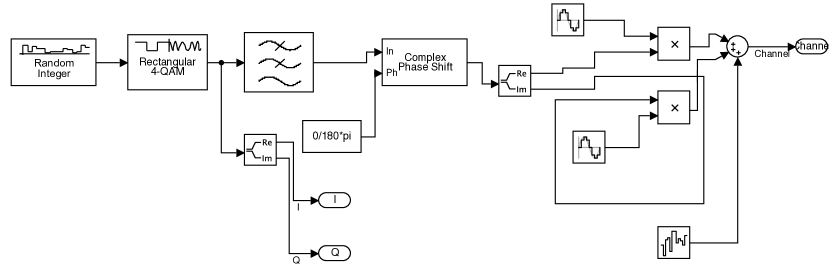
Figure 11: QPSK signal generator

QPSK Signal generator is composed of Simulink standard library. Random integer block generate digital data, which is then converted to QPSK signal by “Rectangular 4-QAM” block, and low-pass filtered by “Low-pass RF filter”. Low-pass filtered signal is then phase-shifted by $180$ degrees and multiplied by carrier (separately Re and Im parts of complex signal). Small noise is added to resulting signal (“Band-limited white noise” block).

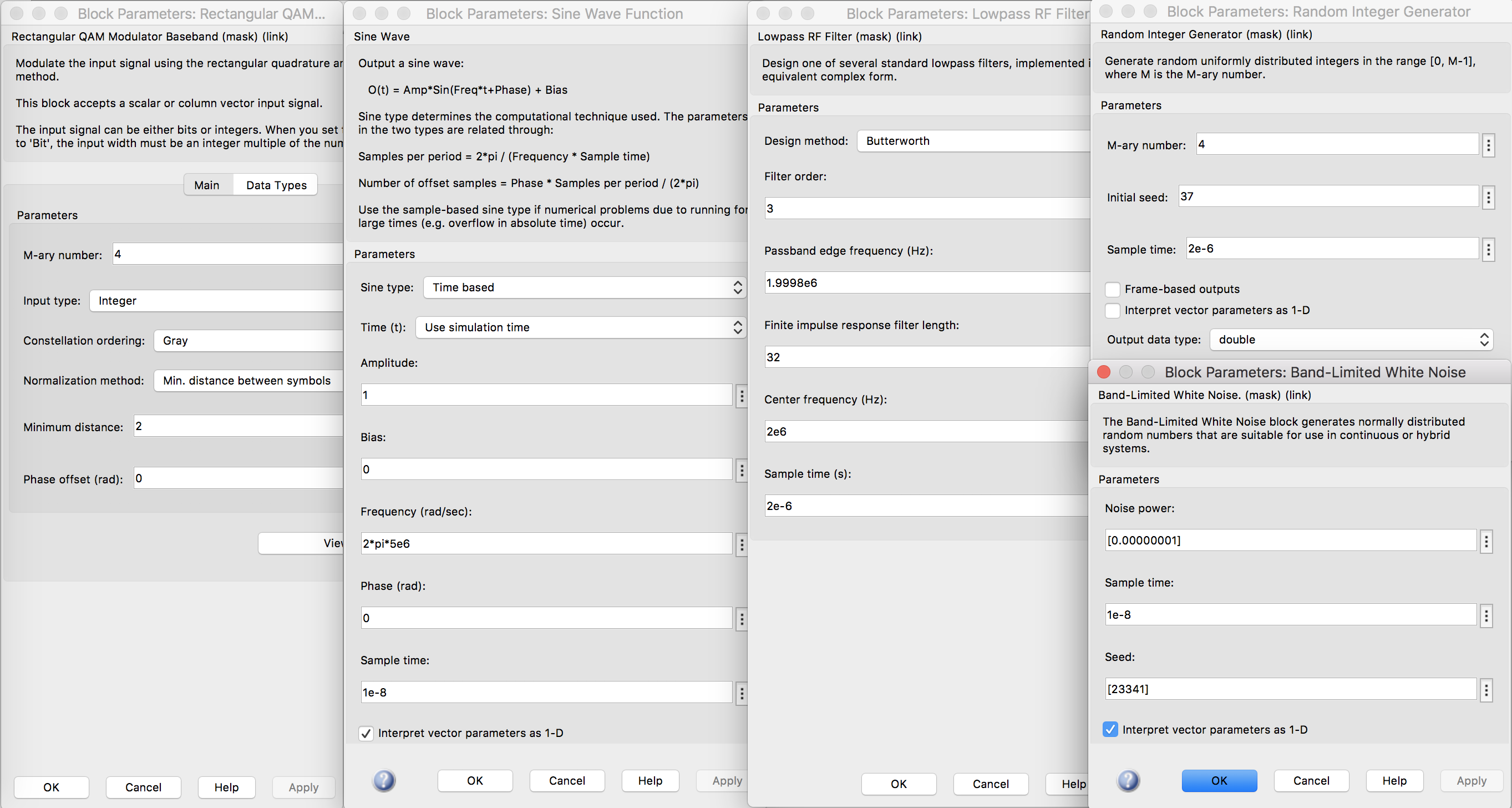
Figure 12: QPSK signal generator: parameters

Corresponding block-parameters are shown in Fig. 12.

Structure of signal demodulator is not the purpose of this study, therefore here we describe only some example without detailed description.

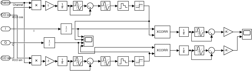
Figure 13: QPSK signal demodulator

Signal demodulator multiplies input QPSK signal by the $\sin$ and $\cos$ carriers, recovered by Costas loop. Resulting signal is flipped (gain block “$-1$”) and integrated ($\frac{1}{s}$ block). After that simple filter is used to obtain moments of switching between $0$ and $1$ (delay and difference blocks). Next, corresponding signals are converted to digital domain by “Zero-Order Hold” and “Sign” blocks. Finally, obtained digital signals are compared with original $I$ and $Q$ digital data signals (“XCORR” correlation block, digital filter, and gain blocks).

Consider now classic QPSK Costas loop (fig. 1) in Matlab Simulink in Fig. 14.

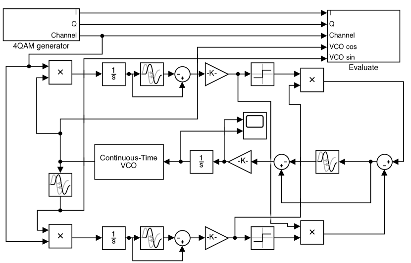
Figure 14: Classic QPSK Costas loop

Blocks “4QAM generator” and “Evaluate” are described above. Here VCO has single output, and 90 phase-shifter is realized by delay block. Multiplier block is self-explanatory. Low-pass filters consist of integration and delay blocks.

Consider 4th power variation of Costas loop in Matlab Simulink (Fig. 15).

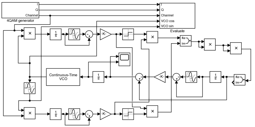
Figure 15: 4th power QPSK Costas loop

This model is constructed similar to classic QPSK Costas loop. The 4th power blocks are realized by two multipliers.

Finally, Matlab Simulink model for folding QPSK Costas loop is shown in Fig. 16.

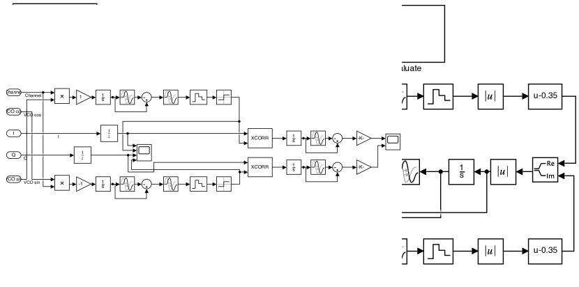
Figure 16: Folding QPSK Costas loop

Here $|\cdot|$ block is standard abs block with enabled zero-crossing detection and bias block centers its input.

4 Conclusions

For conclusion consider comparative graph of signal-to-noise analysis of all three Costas loops (see Fig. 17).

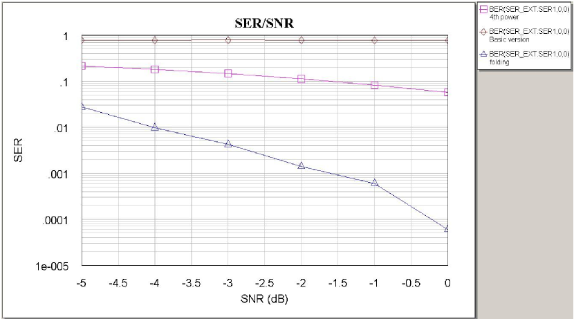
Figure 17: Symbol error rate (SER) comparison in NI AWR Design Environment

Three modifications of 4QAM(QPSK) Costas loops are considered. Simplified version of folding variant is presented for the first time. Hold-in, pull-in, and lock-in ranges for PI loop filters are computed. It is shown that the folding modification works better in the presence of noise. More sophisticated noise analysis is given in [27].

More rigorous mathematical models of the QPSK Costas loop circuits consist of 4th order non-linear differential equations and corresponding lock-in ranges can be estimated numerically similar to [10, 28].

References

- [1] Ahamed, S., Lawrence, V.: Design and Engineering of Intelligent Communication Systems. Springer (1997)
- [2] Meystel, A., Meystel, A., Albus, J.: Intelligent systems: architecture, design, and control. Wiley (2002)
- [3] Sarma, K., Sarma, M., Sarma, M.: Recent Trends in Intelligent and Emerging Systems. Springer India (2015)
- [4] Costas, J.P.: Receiver for communication system (1962). US Patent 3,047,659
- [5] Best, R., Kuznetsov, N., Leonov, G., Yuldashev, M., Yuldashev, R.: Tutorial on dynamic analysis of the Costas loop. Annual Reviews in Control 42, 27–49 (2016). 10.1016/j.arcontrol.2016.08.003
- [6] Best, R.E.: Costas Loops: Theory, Design, and Simulation. Springer International Publishing (2018)
- [7] Gardner, F.: Phaselock techniques. John Wiley & Sons, New York (1966)
- [8] Gardner, F.: Phaselock techniques, 2nd edn. John Wiley & Sons, New York (1979)
- [9] Kuznetsov, N., Leonov, G., Yuldashev, M., Yuldashev, R.: Rigorous mathematical definitions of the hold-in and pull-in ranges for phase-locked loops. IFAC-PapersOnLine 48(11), 710–713 (2015). 10.1016/j.ifacol.2015.09.272
- [10] Leonov, G., Kuznetsov, N., Yuldashev, M., Yuldashev, R.: Hold-in, pull-in, and lock-in ranges of PLL circuits: rigorous mathematical definitions and limitations of classical theory. IEEE Transactions on Circuits and Systems–I: Regular Papers 62(10), 2454–2464 (2015). 10.1109/TCSI.2015.2476295
- [11] Best, R., Kuznetsov, N., Leonov, G., Yuldashev, M., Yuldashev, R.: Simulation of analog Costas loop circuits. International Journal of Automation and Computing 11(6), 571–579 (2014). 10.1007/s11633-014-0846-x
- [12] Leonov, G., Kuznetsov, N., Yuldashev, M., Yuldashev, R.: Nonlinear dynamical model of Costas loop and an approach to the analysis of its stability in the large. Signal Processing 108, 124–135 (2015). 10.1016/j.sigpro.2014.08.033
- [13] Best, R., Kuznetsov, N., Kuznetsova, O., Leonov, G., Yuldashev, M., Yuldashev, R.: A short survey on nonlinear models of the classic Costas loop: rigorous derivation and limitations of the classic analysis. In: Proceedings of the American Control Conference, pp. 1296–1302. IEEE (2015). 10.1109/ACC.2015.7170912. art. num. 7170912
- [14] Ladvánszky, J.: A costas loop variant for large noise. Journal of Asian Scientific Research 8(3), 144–151 (2018)
- [15] Ladvánszky, J., Kovács, G.: Software based separation of amplitude and phase noises in time domain. In: Circuits and Systems (ISCAS), 2011 IEEE International Symposium on, pp. 769–772. IEEE (2011)
- [16] Piqueira, J., Monteiro, L.: Considering second-harmonic terms in the operation of the phase detector for second-order phase-locked loop. IEEE Transactions On Circuits And Systems-I 50(6), 805–809 (2003)
- [17] Leonov, G., Kuznetsov, N., Yuldashev, M., Yuldashev, R.: Analytical method for computation of phase-detector characteristic. IEEE Transactions on Circuits and Systems - II: Express Briefs 59(10), 633–647 (2012). 10.1109/TCSII.2012.2213362
- [18] Leonov, G., Kuznetsov, N., Yuldashev, M., Yuldashev, R.: Computation of the phase detector characteristic of a QPSK Costas loop. Doklady Mathematics 93(3), 348–353 (2016). 10.1134/S1064562416030236
- [19] Weber, C.L.: Candidate receivers for unbalanced qpsk. In: International Telemetering Conference Proceedings. International Foundation for Telemetering (1976)
- [20] Osborne, H.: A generalized “polarity-type” Costas loop for tracking MPSK signals. IEEE Transactions on Communications 30(10), 2289–2296 (1982)
- [21] Barry, J.R., Kahn, J.M.: Carrier synchronization for homodyne and heterodyne detection of optical quadriphase-shift keying. Journal of lightwave technology 10(12), 1939–1951 (1992)
- [22] Ladvánszky, J., Covács, B.: Methods and apparatus for signal demodulation. Patent application P74032. Ericsson inc. (2018)
- [23] Kuznetsov, N., Leonov, G., Yuldashev, M., Yuldashev, R.: Solution of the Gardner problem on the lock-in range of phase-locked loop. ArXiv e-prints (2017). 1705.05013
- [24] Aleksandrov, K., Kuznetsov, N., Leonov, G., Yuldashev, M., Yuldashev, R.: Lock-in range of PLL-based circuits with proportionally-integrating filter and sinusoidal phase detector characteristic. arXiv preprint arXiv:1603.08401 (2016)
- [25] Aleksandrov, K., Kuznetsov, N., Leonov, G., Yuldashev, M., Yuldashev, R.: Lock-in range of classical PLL with impulse signals and proportionally-integrating filter. arXiv preprint arXiv:1603.09363 (2016)
- [26] Ladvánszky, J.: A Costas loop variant for large noise (patent application) (2017)
- [27] Sidorkina, Y., Sizykh, V., Shakhtarin, B.I., Shevtsev, V.: Costas circuit under the action of additive harmonic interferences and wideband noise. Journal of Communications Technology and Electronics 61(7), 807–816 (2016)
- [28] Kuznetsov, N., Kuznetsova, O., Leonov, G., Yuldashev, M., Yuldashev, R.: A short survey on nonlinear models of QPSK Costas loop. IFAC-PapersOnLine 50(1), 6525 – 6533 (2017)