Differentially Private Contextual Linear Bandits

Abstract

We study the contextual linear bandit problem, a version of the standard stochastic multi-armed bandit (MAB) problem where a learner sequentially selects actions to maximize a reward which depends also on a user provided per-round context. Though the context is chosen arbitrarily or adversarially, the reward is assumed to be a stochastic function of a feature vector that encodes the context and selected action. Our goal is to devise private learners for the contextual linear bandit problem.

We first show that using the standard definition of differential privacy results in linear regret. So instead, we adopt the notion of joint differential privacy, where we assume that the action chosen on day $t$ is only revealed to user $t$ and thus needn’t be kept private that day, only on following days. We give a general scheme converting the classic linear-UCB algorithm into a joint differentially private algorithm using the tree-based algorithm [10, 18]. We then apply either Gaussian noise or Wishart noise to achieve joint-differentially private algorithms and bound the resulting algorithms’ regrets. In addition, we give the first lower bound on the additional regret any private algorithms for the MAB problem must incur.

1 Introduction

The well-known stochastic multi-armed bandit (MAB) is a sequential decision-making task in which a learner repeatedly chooses an action (or arm) and receives a noisy reward. The objective is to maximize cumulative reward by exploring the actions to discover optimal ones (having the best expected reward), balanced with exploiting them. The contextual bandit problem is an extension of the MAB problem, where the learner also receives a context in each round, and the expected reward depends on both the context and the selected action.

As a motivating example, consider online shopping: the user provides a context (composed of query words, past purchases, etc.), and the website responds with a suggested product and receives a reward if the user buys it. Ignoring the context and modeling the problem as a standard MAB (with an action for each possible product) suffers from the drawback of ignoring the variety of users’ preferences; whereas separately learning each user’s preferences doesn’t allow us to generalize between users. Therefore it is common to model the task as a contextual linear bandit problem: Based on the user-given context, each action is mapped to a feature vector; the reward probability is then assumed to depend on the same unknown linear function of the feature vector across all users.

The above example motivates the need for privacy in the contextual bandit setting: users’ past purchases and search queries are sensitive personal information, yet they strongly predict future purchases. In this work, we give upper and lower bounds for the problem of (joint) differentially private contextual linear bandits. Differential privacy is the de facto gold standard of privacy-preserving data analysis in both academia and industry, requiring that an algorithm’s output have very limited dependency on any single user interaction (one context and reward). However, as we later illustrate, adhering to the standard notion of differential privacy (under event-level continual observation) in the contextual bandit requires us to essentially ignore the context and thus incur linear regret. We therefore adopt the more relaxed notion of joint differential privacy [23] which, intuitively, allows us to present the $t$-th user with products corresponding to her preferences, while guaranteeing that all interactions with all users at times $t^{\prime}>t$ have very limited dependence on user $t$’s preferences. The guarantee of differential privacy under continuous observation assures us that even if all later users collude in an effort to learn user $t$’s context or preference, they still have very limited advantage over a random guess.

1.1 Problem Formulation

Stochastic Contextual Linear Bandits.

In the classic MAB, in every round $t$ a learner selects an action $a_{t}$ from a fixed set $\mathcal{A}$ and receives a reward $y_{t}$. In the (stationary) stochastic MAB, the reward is noisy with a fixed but unknown expectation $\mathds{E}[y_{t}\nonscript\>|\allowbreak\nonscript\>\mathopen{}a_{t}]$ that depends only on the selected action. In the stochastic contextual bandit problem, before each round the learner also receives a context $c_{t}\in\mathcal{C}$ — the expected reward $\mathds{E}[y_{t}\nonscript\>|\allowbreak\nonscript\>\mathopen{}c_{t},a_{t}]$ depends on both $c_{t}$ and $a_{t}$. It is common to assume that the context affects the reward in a linear way: map every context-action pair to a feature vector $\phi(c,a)\in\mathds{R}^{d}$ (where $\phi$ is an arbitrary but known function) and assume that $\mathds{E}[y_{t}\nonscript\>|\allowbreak\nonscript\>\mathopen{}c_{t},a_{t}]=\langle\bm{\theta}^{*},\phi(c_{t},a_{t})\rangle$. The vector $\bm{\theta}^{*}\in\mathds{R}^{d}$ is the key unknown parameter of the environment which the learner must discover to maximize reward. Alternatively, we say that on every round the learner is given a decision set $\mathcal{D}_{t}\coloneq\{\phi(c_{t},a)\nonscript\>|\allowbreak\nonscript\>\mathopen{}a\in\mathcal{A}\}$ of all the pre-computed feature vectors: choosing $\bm{x}_{t}\in\mathcal{D}_{t}$ effectively determines the action $a_{t}\in\mathcal{A}$. Thus, the contextual stochastic linear bandit framework consists of repeated rounds in which the learner (i) receives a decision set $\mathcal{D}_{t}\subset\mathds{R}^{d}$ (ii) chooses an action $\bm{x}_{t}\in\mathcal{D}_{t}$ (iii) receives a stochastic reward $y_{t}=\langle\bm{\theta}^{*},\bm{x}_{t}\rangle+\eta_{t}$. When all the $\mathcal{D}_{t}$ are identical and consist of the standard basis vectors, the problem reduces to standard MAB.

The learner’s objective is to maximize cumulative reward, which is equivalent to minimizing regret: the extra reward a learner would have received by always choosing the best available action. In other words, the regret characterizes the cost of having to learn the optimal action over just knowing it beforehand. For stochastic problems, we are usually interested in a related quantity called pseudo-regret, which is the extra expected reward that the learner could have earned if it had known $\bm{\theta}^{*}$ in advance. In our setting, the cumulative pseudo-regret after $n$ rounds is $\widehat{R}_{n}\coloneq\sum_{t=1}^{n}\max_{\bm{x}\in\mathcal{D}_{t}}\langle\bm{\theta}^{*},\bm{x}-\bm{x}_{t}\rangle$.

Joint Differential Privacy.

As discussed above, the context and reward may be considered private information about the users which we wish to keep private from all other users. We thus introduce the notion of jointly differentially private learners under continuous observation, a combination of two definitions [given in 23, 18]. First, we say two sequences $S=\langle(\mathcal{D}_{1},y_{1}),(\mathcal{D}_{2},y_{2}),\dotsc,(\mathcal{D}_{n},y_{n})\rangle$ and $S^{\prime}=\langle(\mathcal{D}^{\prime}_{1},y^{\prime}_{1}),\dotsc,(\mathcal{D}^{\prime}_{n},y^{\prime}_{n})\rangle$ are $t$-neighbors if for all $t^{\prime}\neq t$ it holds that $(\mathcal{D}_{t^{\prime}},y_{t^{\prime}})=(\mathcal{D}^{\prime}_{t^{\prime}},y^{\prime}_{t^{\prime}})$.

Definition 1.

A randomized algorithm $A$ for the contextual bandit problem is $(\varepsilon,\delta)$-jointly differentially private (JDP) under continual observation if for any $t$ and any pair of $t$-neighboring sequences $S$ and $S^{\prime}$, and any subset ${\cal S}_{>t}\subset\mathcal{D}_{t+1}\times\mathcal{D}_{t+2}\times\dotsb\times\mathcal{D}_{n}$ of sequence of actions ranging from day $t+1$ to the end of the sequence, it holds that $\mathds{P}\lparen A(S)\in\mathcal{S}_{>t}\rparen\leq e^{\varepsilon}\mathds{P}\lparen A(S^{\prime})\in\mathcal{S}^{\prime}_{>t}\rparen+\delta$.

The standard notion of differential privacy under continual observation would require that changing the context $c_{t}$ cannot have much effect on the probability of choosing action $a_{t}$ — even for round $t$ itself (not just for future rounds as with JDP). In our problem formulation, however, changing $c_{t}$ to $c_{t}^{\prime}$ may change the decision set $\mathcal{D}_{t}$ to a possibly disjoint $\mathcal{D}_{t}^{\prime}$, making that notion ill-defined. Therefore, when we discuss the impossibility of regret-minimization under standard differential privacy in Section 5, we revert back to a fixed action set $\mathcal{A}$ with an explicit per-round context $c_{t}$.

1.2 Our Contributions and Paper Organization

In this work, in addition to formulating the definition of JDP under continual observation, we also present a framework for implementing JDP algorithms for the contextual linear bandit problem. Not surprisingly, our framework combines a tree-based privacy algorithm [10, 18] with a linear upper confidence bound (LinUCB) algorithm [13]. For modularity, in Section 3 we analyze a family of linear UCB algorithms that use different regularizers in every round, under the premise that the regularizers are PSD with bounded singular values. Moreover, we repeat our analysis twice — first we obtain a general $\tilde{O}(\sqrt{n})$ upper bound on regret; then, for problem instances that maintain a $\Delta$ reward gap separating the optimal and sub-optimal actions, we obtain a $\mathrm{polylog}(n)/\Delta$ regret upper bound. Our leading application of course is privacy, though one could postulate other reasons where such changing regularizers would be useful (e.g., if parameter estimates turn out to be wrong and have to be updated). We then plug two particular regularizers into our scheme: the first is a privacy-preserving mechanism that uses additive Wishart noise [30] (which is always PSD); the second uses additive Gaussian noise [19] (shifted to make it PSD w.h.p. over all rounds). The main term in the two regret bounds obtained by both algorithms is $\tilde{O}(\sqrt{n}\cdot d^{3/4}/\sqrt{\varepsilon})$ (the bound itself depends on numerous parameters, a notation-list given in Section 2). Details of both techniques appear in Section 4. Experiments with a few variants of our algorithms are detailed in Appendix D of the supplementary material. In Section 5 we also give a lower bound for the $\varepsilon$-differentially private MAB problem. Whereas all previous work on the private MAB problem uses standard (non-private) bounds, we show that any private algorithm must incur an additional regret of $\Omega(k\log(n)/\varepsilon)$. While the result resembles the lower bound in the adversarial setting, the proof technique cannot rely on standard packing arguments [e.g. 20] since the input for the problem is stochastic rather than adversarial. Instead, we rely on a recent coupling argument [22] to prove any private algorithm must substantially explore suboptimal arms.

Future Directions.

The linear UCB algorithm we adapt in this work is a canonical approach to the linear bandit problem, using the principle of “optimism in the face of uncertainty.” However, recent work [24] shows that all such “optimistic” algorithms are sub-optimal, and instead proposes adapting to the decision set in a particular way by solving an intricate optimization problem. It remains an open question to devise a private version of this algorithm which interpolates between UCB and fine-tuning to the specific action set.

1.3 Related Work

MAB and the Contextual Bandit Problem.

The MAB dates to the seminal work of Robbins [28], with the UCB approach developed in a series of works [8, 4] culminating in [6]. Stochastic linear bandits were formally first introduced in [3], and [5] was the first paper to consider UCB-style algorithms. An algorithm that is based on a confidence ellipsoid is described by [13], with a variant based on ridge regression given in [12], or explore-then-commit variant in [29], and a variant related to a sparse setting appears in [2]. Abbasi-Yadkori et al. [1] gives an instance dependent bound for linear bandits, which we convert to the contextual setting.

Differential Privacy.

Differential privacy, first introduced by Dwork et al. [17, 16], is a rigorous mathematical notion of privacy that requires the probability of any observable output to change very little when any single datum changes. (We omit the formal definition, having already defined JDP.) Among its many elegant traits is the notion of group privacy: should $k$ datums change then the change in the probability of any event is still limited by (roughly) $k$ times the change when a single datum was changed. Differential privacy also composes: the combination of $k$ $(\varepsilon,\delta)$-differentially private algorithms is $\big{\lparen}O(k\varepsilon^{2}+2\sqrt{k\log(\nicefrac{{1}}{{\delta^{\prime}}})}),k\delta+\delta^{\prime}\big{\rparen}$-differentially private for any $\delta^{\prime}>0$ [14].

The notion of differential privacy under continual observation was first defined by Dwork et al. [18] using the tree-based algorithm [originally appearing in 10]. This algorithm maintains a binary tree whose $n$ leaves correspond to the $n$ entries in the input sequence. Each node in the tree maintains a noisy (privacy-preserving) sum of the input entries in its subtree — the cumulative sums of the inputs can thus be obtained by combining at most $\log(n)$ noisy sums. This algorithm is the key ingredient of a variety of works that deal with privacy in an online setting, including counts [18], online convex optimization [21], and regret minimization in both the adversarial [31, 34] and stochastic [26, 33] settings. We comment that Mishra and Thakurta [26] proposed an algorithm similar to our own for the contextual bandit setting, however (i) without maintaining PSD, (ii) without any analysis, only empirical evidence, and (iii) without presenting lower bounds. A partial utility analysis of this algorithm, in the reward-privacy model (where the context’s privacy is not guaranteed), appears in the recent work of Neel and Roth [27]. Further details about achieving differential privacy via additive noise and the tree-based algorithm appear in Appendix A of the supplementary material. The related problem of private linear regression has also been extensively studied in the offline setting [11, 7].

2 Preliminaries and Notation

We use $\bm{bold}$ letters to denote vectors and bold $\bm{CAPITALS}$ for matrices. Given a $d$-column matrix $\bm{M}$, its Gram matrix is the $(d\times d)$-matrix $\bm{M}^{\top}{\bm{M}}$. A symmetric matrix $\bm{M}$ is positive-semidefinite (PSD, denoted $\bm{M}\succeq 0$) if $\bm{x}^{\top}\bm{M}\bm{x}\geq 0$ for any vector $\bm{x}$. Any such $\bm{M}$ defines a norm on vectors, so we define $\|x\|_{M}^{2}=\bm{x}^{\top}\bm{M}\bm{x}$. We use $\bm{M}\succeq\bm{N}$ to mean $\bm{M}-\bm{N}\succeq 0$. The Gaussian distribution $\mathcal{N}(\mu,\sigma^{2})$ is defined by the density function ${(2\pi\sigma^{2})}^{\nicefrac{{-1}}{{2}}}\exp(\nicefrac{{-{(x-\mu)}^{2}}}{{2\sigma^{2}}})$. The squared $L_{2}$-norm of a $d$-dimensional vector whose coordinates are drawn i.i.d. from $\mathcal{N}(0,1)$ is given by the $\chi^{2}(d)$ distribution, which is tightly concentrated around $d$. Given two distributions $\mathds{P}$ and $\mathds{Q}$ we denote their total variation distance by $d_{\rm TV}(\mathds{P},\mathds{Q})=\max_{\text{event }E}|\mathds{P}\lparen E\rparen-{\mathds{Q}}(E)|$.

Notation.

Our bound depends on many parameters of the problem, specified below. Additional parameters (bounds) are specified in the assumptions stated below.

$n$

horizon, i.e. number of rounds

$s,t$

indices of rounds

$d$

dimensionality of action space

$\mathcal{D}_{t}$

$\subset\mathds{R}^{d}$; decision set at round $t$

$\bm{x}_{t}$

$\in\mathcal{D}_{t}$; action at round $t$

$y_{t}$

$\in\mathds{R}$; reward at round $t$

$\bm{\theta}^{*}$

$\in\mathds{R}^{d}$; unknown parameter vector

$m$

$\coloneq\lceil\log_{2}(n)+1\rceil$

$\bm{X}_{<t}$

$\in\mathds{R}^{(t-1)\times d}$, with $\bm{X}_{<t,s}=\bm{x}_{s}^{\top}$ for $s<t$

$\bm{G}_{t}$

Gram matrix of the actions: $\bm{X}_{<t}^{\top}{\bm{X}_{<t}}$

$\bm{H}_{t}$

regularizer at round $t$

$\bm{y}_{<t}$

vector of rewards up to round $t-1$

$\bm{u}_{t}$

action-reward product: $\bm{X}_{<t}^{\top}\bm{y}_{<t}$

$\bm{h}_{t}$

perturbation of $\bm{u}_{t}$

3 Linear UCB with Changing Regularizers

In this section we introduce and analyze a variation of the well-studied LinUCB algorithm, an application of the Upper Confidence Bound (UCB) idea to stochastic linear bandits [13, 29, 1]. At every round $t$, LinUCB constructs a confidence set $\mathcal{E}_{t}$ that contains the unknown parameter vector $\bm{\theta}^{*}$ with high probability. It then computes an upper confidence bound on the reward of each action in the decision set $\mathcal{D}_{t}$, and “optimistically” chooses the action with the highest UCB: $\bm{x}_{t}\leftarrow\operatorname*{arg\,max}_{\bm{x}\in\mathcal{D}_{t}}\mathrm{UCB}_{t}(\bm{x})$, where $\mathrm{UCB}_{t}(\bm{x})\coloneq\max_{\bm{\theta}\in\mathcal{E}_{t}}\langle\bm{\theta},\bm{x}\rangle$. We assume the rewards are linear with added subgaussian noise (i.e., $y_{s}=\langle\bm{\theta}^{*},\bm{x}_{s}\rangle+\eta_{s}$ for $s<t$), so it is natural to center the confidence set $\mathcal{E}_{t}$ on the (regularized) linear regression estimate:

$$\hat{\bm{\theta}}_{t} \coloneq\operatorname*{arg\,min}_{\hat{\bm{\theta}}\in\mathds{R}^{d}}\|\bm{X}_{<t}\hat{\bm{\theta}}-\bm{y}_{<t}\|^{2}+\|\hat{\bm{\theta}}\|_{\bm{H}_{t}}^{2}=(\bm{G}_{t}+\bm{H}_{t})^{-1}\bm{X}_{<t}^{\top}\bm{y}_{<t}. \text{where }\bm{G}_{t}\coloneq\bm{X}_{<t}^{\top}{\bm{X}_{<t}}$$

The matrix $\bm{V}_{t}\coloneq\bm{G}_{t}+\bm{H}_{t}\in\mathds{R}^{d\times d}$ is a regularized version of the Gram matrix $\bm{G}_{t}$. Whenever the learner chooses an action vector $\bm{x}\in\mathcal{D}_{t}$, the corresponding reward gives it some information about the projection of $\bm{\theta}^{*}$ onto $\bm{x}$. In other words, the estimate $\hat{\bm{\theta}}$ is probably closer to $\bm{\theta}^{*}$ along the directions where many actions have been taken. This motivates the use of ellipsoidal confidence sets that are smaller in such directions, inversely corresponding to the eigenvalues of $\bm{G}_{t}$ (or $\bm{V}_{t}$). The ellipsoid is uniformly scaled by $\beta_{t}$ to achieve the desired confidence level, as prescribed by Proposition 4.

$$\mathcal{E}_{t} \coloneq\{\bm{\theta}\in\mathds{R}^{d}\nonscript\>|\allowbreak\nonscript\>\mathopen{}\|\bm{\theta}-\hat{\bm{\theta}}_{t}\|_{\bm{V}_{t}}\leq\beta_{t}\}, \text{for which }\mathrm{UCB}_{t}(\bm{x}) =\langle\hat{\bm{\theta}},\bm{x}\rangle+\beta_{t}\|\bm{x}\|_{\bm{V}_{t}^{-1}}.$$ (1)

Just as the changing regularizer $\bm{H}_{t}$ perturbs the Gram matrix $\bm{G}_{t}$, our algorithm allows for the vector $\bm{u}_{t}\coloneq\bm{X}_{<t}^{\top}\bm{y}_{<t}$ to be perturbed by $\bm{h}_{t}$ to get $\tilde{\bm{u}}_{t}\coloneq\bm{u}_{t}+\bm{h}_{t}$. The estimate $\hat{\bm{\theta}}_{t}$ is replaced by $\tilde{\bm{\theta}}_{t}\coloneq\bm{V}_{t}^{-1}\tilde{\bm{u}}_{t}$.

Algorithm 1 Linear UCB with Changing Perturbations

Initialize: $\bm{G}_{1}\leftarrow\bm{0}_{d\times d}$, $u_{1}\leftarrow\bm{0}_{d}$.

for each round $t=1,2,\dotsc,n$ do

      Receive $\mathcal{D}_{t}\leftarrow{}$ decision set ${}\subset\mathds{R}^{d}$.

      Receive regularized $\bm{V}_{t}\leftarrow\bm{G}_{t}+\bm{H}_{t}$ and perturbed $\tilde{\bm{u}}_{t}\leftarrow\bm{u}_{t}+\bm{h}_{t}$

      Compute regressor $\tilde{\bm{\theta}}_{t}\leftarrow\bm{V}_{t}^{-1}\tilde{\bm{u}}_{t}$

      Compute confidence-set bound $\beta_{t}$ based on Proposition 4.

      Pick action $\bm{x}_{t}\leftarrow\operatorname*{arg\,max}_{\bm{x}\in\mathcal{D}_{t}}\langle\tilde{\bm{\theta}}_{t},\bm{x}\rangle+\beta_{t}\|\bm{x}\|_{\bm{V}_{t}^{-1}}$.

      Observe $y_{t}\leftarrow{}$ reward for action $\bm{x}_{t}$

      Update: $\bm{G}_{t+1}\leftarrow\bm{G}_{t}+\bm{x}_{t}\bm{x}_{t}^{\top},\quad\bm{u}_{t+1}\leftarrow\bm{u}_{t}+\bm{x}_{t}y_{t}$

end for

Our analysis relies on the following assumptions about the environment and algorithm:

Assumptions (Algorithm 1).

For all rounds $t=1,\dotsc,n$ and actions $\bm{x}\in\mathcal{D}_{t}$:

1. Bounded action set: $\|\bm{x}\|\leq L$.

2. Bounded mean reward: $|\langle\bm{\theta}^{*},\bm{x}\rangle|\leq B$ with $B\geq 1$.

3. Bounded target parameter: $\|\bm{\theta}^{*}\|\leq S$.

4. All regularizers are PSD $\bm{H}_{t}\succeq 0$.

5. $y_{t}=\langle\bm{\theta}^{*},\bm{x}_{t}\rangle+\eta_{t}$ where $\eta_{t}$ is $\sigma^{2}$-conditionally subgaussian on previous actions and rewards, i.e.: $\mathds{E}[\exp(\lambda\eta_{t})\nonscript\>|\allowbreak\nonscript\>\mathopen{}\bm{x}_{1},y_{1},\dotsc,\bm{x}_{t-1},y_{t-1},\bm{x}_{t}]\leq\exp(\lambda^{2}\sigma^{2}/2)$, for all $\lambda\in\mathds{R}$.

6. Strongest bound on both the action and the reward: $\|\bm{x}_{t}\|^{2}+y_{t}^{2}\leq\tilde{L}^{2}$ for all rounds $t$. In particular, if $\|\bm{x}_{t}\|\leq L$ (Item 1) and the rewards are bounded: $|y_{t}|\leq\tilde{B}$ (not just their means as in Item 2), we can set $\tilde{L}^{2}=L^{2}+\tilde{B}^{2}$.

Items 1 and 2 aren’t required to have good pseudo-regret bounds, they merely simplify the bounds on the confidence set (see Proposition 4 and Section 3.1). Item 6 is not required at all for now, it is only used for joint differential privacy in Section 4.

To fully describe Algorithm 1 we need to specify how to compute the confidence-set bounds ${(\beta_{t})}_{t}$. On the one hand, these bounds have to be accurate — the confidence set $\mathcal{E}_{t}$ should contain the unknown $\bm{\theta}^{*}$; on the other hand, the larger they are, the larger the regret bounds we obtain. In other words, the $\beta_{t}$ should be as small as possible subject to being accurate.

Definition 2 (Accurate ${(\beta_{t})}_{t}$).

A sequence ${(\beta_{t})}_{t=1}^{n}$ is $(\alpha,n)$-accurate for ${(\bm{H}_{t})}_{t=1}^{n}$ and ${(\bm{h}_{t})}_{t=1}^{n}$ if, with probability at least $1-\alpha$, it satisfies $\|\bm{\theta}^{*}-\tilde{\bm{\theta}}_{t}\|_{\bm{V}_{t}}\leq\beta_{t}$ for all rounds $t=1,\dotsc,n$ simultaneously.

We now argue that three parameters are the key to establishing accurate confidence-set bounds ${(\beta_{t})}_{t=1}^{n}$ — taking into account the noise in the setting and the noise added by a changing $\bm{H}_{t}$ and $\bm{h}_{t}$.

Definition 3 (Accurate $\rho_{\min}$, $\rho_{\max}$, and $\gamma$).

The bounds $0<\rho_{\min}\leq\rho_{\max}$ and $\gamma$ are $(\alpha/2n)$-accurate for ${(\bm{H}_{t})}_{t=1}^{n}$ and ${(\bm{h}_{t})}_{t=1}^{n}$ if for each round $t$:

$$\|\bm{H}_{t}\| \leq\rho_{\max}, \|\bm{H}_{t}^{-1}\| \leq 1/\rho_{\min}, \|\bm{h}_{t}\|_{\bm{H}_{t}^{-1}} \leq\gamma; \text{with probability at least }1-\alpha/2n.$$

Proposition 4 (Calculating $\beta_{t}$).

Suppose Items 3, 4 and 5 hold and let $\rho_{\min}$, $\rho_{\max}$, and $\gamma$ be $(\alpha/2n)$-accurate for some $\alpha\in(0,1)$ and horizon $n$. Then ${(\beta_{t})}_{t=1}^{n}$ is $(\alpha,n)$-accurate where

$$\beta_{t} \coloneq\sigma\sqrt{2\log(2/\alpha)+\log(\operatorname{det}\bm{V}_{t})-d\log(\rho_{\min})}+S\sqrt{\rho_{\max}}+\gamma$$

$$\leq\sigma\sqrt{2\log({2}/{\alpha})+d\log\Big{\lparen}\tfrac{\rho_{\max}}{\rho_{\min}}+\tfrac{tL^{2}}{d\rho_{\min}}\Big{\rparen}}+S\sqrt{\rho_{\max}}+\gamma.$$ (if Item 1 also holds)

3.1 Regret Bounds

We now present bounds on the maximum regret of Algorithm 1. However, due to space constraints, we defer an extensive discussion of the proof techniques used and the significance of the results to Appendix B in the supplementary material. The proofs are based on those of Abbasi-Yadkori et al. [1], who analyzed LinUCB with constant regularizers. On one hand, our changes are mostly technical; however, it turns out that various parts of the proof diverge and now depend on $\rho_{\max}$ and $\rho_{\min}$; tracing them all is somewhat involved. It is an interesting question to establish similar bounds using known results only as a black box; we were not able to accomplish this.

Theorem 5 (Regret of Algorithm 1).

Suppose Items 1, 2, 3, 4 and 5 hold and the $\beta_{t}$ are as given by Proposition 4. Then with probability at least $1-\alpha$ the pseudo-regret of Algorithm 1 is bounded by

$$\widehat{R}_{n} \leq B\sqrt{8n}\bigg{[}\sigma\left\lparen 2\log(\tfrac{2}{\alpha})+d\log\left\lparen\tfrac{\rho_{\max}}{\rho_{\min}}+\tfrac{nL^{2}}{d\rho_{\min}}\right\rparen\right\rparen+(S\sqrt{\rho_{\max}}+\gamma)\sqrt{d\log\left\lparen 1+\tfrac{nL^{2}}{d\rho_{\min}}\right\rparen}\bigg{]}$$ (2)

Theorem 6 (Gap-Dependent Regret of Algorithm 1).

Suppose Items 1, 2, 3, 4 and 5 hold and the $\beta_{t}$ are as given by Proposition 4. If the optimal actions in every decision set $\mathcal{D}_{t}$ are separated from the sub-optimal actions by a reward gap of at least $\Delta$, then with probability at least $1-\alpha$ the pseudo-regret of Algorithm 1 satisfies

$$\widehat{R}_{n} \leq\frac{8B}{\Delta}\bigg{[}\sigma\left\lparen 2\log(\tfrac{2}{\alpha})+d\log\left\lparen\tfrac{\rho_{\max}}{\rho_{\min}}+\tfrac{nL^{2}}{d\rho_{\min}}\right\rparen\right\rparen+(S\sqrt{\rho_{\max}}+\gamma)\sqrt{d\log\left\lparen 1+\tfrac{nL^{2}}{d\rho_{\min}}\right\rparen}\bigg{]}^{2}$$ (3)

4 Linear UCB with Joint Differential Privacy

Notice that Algorithm 1 uses its history of actions and rewards up to round $t$ only via the confidence set $\mathcal{E}_{t}$, which is to say via $\bm{V}_{t}$ and $\tilde{\bm{u}}_{t}$, which are perturbations of the Gram matrix $\bm{G}_{t}$ and the vector $\bm{u}_{t}\coloneq\bm{X}_{<t}^{\top}\bm{y}_{<t}$, respectively; these also determine $\beta_{t}$. By recording this history with differential privacy, we obtain a Linear UCB algorithm that is jointly differentially private (Definition 1) because it simply post-processes $\bm{G}_{t}$ and $\bm{u}_{t}$.

Claim 7 (see Dwork and Roth [15, Proposition 2.1]).

If the sequence ${(\bm{V}_{t},\tilde{\bm{u}}_{t})}_{t=1}^{n-1}$ is $(\varepsilon,\delta)$-differentially private with respect to ${(\bm{x}_{t},y_{t})}_{t=1}^{n-1}$, then Algorithm 1 is $(\varepsilon,\delta)$-jointly differentially private.

Remark 1.

Algorithm 1 is only jointly differentially private even though the history maintains full differential privacy — its action choice depends not only on the past contexts $c_{s}$ ($s<t$, via the differentially private $\bm{X}_{<t}$) but also on the current context $c_{t}$ via the decision set $\mathcal{D}_{t}$. This use of $c_{t}$ is not differentially private, as it is revealed by the algorithm’s chosen $\bm{x}_{t}$.

Rather than applying the tree-based algorithm separately to $\bm{G}_{t}$ and $\bm{u}_{t}$, we aggregate both into the single matrix $\bm{M}_{t}\in\mathds{R}^{(d+1)\times(d+1)}$, which we now construct. Define $\bm{A}\coloneq\begin{bmatrix}\bm{X}_{1:n}&\bm{y}_{1:n}\end{bmatrix}\in\mathds{R}^{n\times(d+1)}$, with $\bm{A}_{t}$ holding the top $t-1$ rows of $\bm{A}$ (and $\bm{A}_{1}=\bm{0}_{1\times(d+1)}$). Now let $\bm{M}_{t}\coloneq\bm{A}_{t}^{\top}{\bm{A}_{t}}$ — then the top-left $d\times d$ sub-matrix of $\bm{M}_{t}$ is the Gram matrix $\bm{G}_{t}$ and the first $d$ entries of its last column are $\bm{u}_{t}$. Furthermore, since $M_{t+1}=M_{t}+\begin{bmatrix}\bm{x}_{t}^{\top}&y_{t}\end{bmatrix}^{\top}{\begin{bmatrix}\bm{x}_{t}^{\top}&y_{t}\end{bmatrix}}$, the tree-based algorithm for private cumulative sums can be used to maintain a private estimation of $\bm{M}_{t}$ using additive noise, releasing $\bm{M}_{t}+\bm{N}_{t}$. The top-left $d\times d$ sub-matrix of $\bm{N}_{t}$ becomes $\bm{H}_{t}$ and the first $d$ entries of its last column become $\bm{h}_{t}$. Lastly, to have a private estimation of $\bm{M}_{t}$, Item 6 must hold.

Below we present two techniques for maintaining (and updating) the private estimations of $\bm{M}_{t}$. As mentioned in Section 1.3, the key component of our technique is the tree-based algorithm, allowing us to estimate $\bm{M}_{t}$ using at most $m\coloneq 1+\lceil\log_{2}n\rceil$ noisy counters. In order for the entire tree-based algorithm to be $(\varepsilon,\delta)$-differentially private, we add noise to each node in the tree so that each noisy count on its own preserves $(\nicefrac{{\varepsilon}}{{\sqrt{8m\ln(\nicefrac{{2}}{{\delta}})}}},\nicefrac{{\delta}}{{2m}})$-differential privacy. Thus in each day, the noise $\bm{N}_{t}$ that we add to $\bm{M}_{t}$ comes from the sum of at most $m$ such counters.

4.1 Differential Privacy via Wishart Noise

First, we instantiate the tree-based algorithm with noise from a suitably chosen Wishart distribution $\mathcal{W}_{d+1}(\bm{V},k)$, which is the result of sampling $k$ independent $(d+1)$-dimensional Gaussians from $\mathcal{N}(\bm{0}_{d+1},\bm{V})$ and computing their Gram matrix.

Theorem 8 (Theorem 4.1 [30]).

Fix positive $\varepsilon_{0}$ and $\delta_{0}$. If the $L_{2}$-norm of each row in the input is bounded by $\tilde{L}$ then releasing the input’s Gram matrix with added noise sampled from $\mathcal{W}_{d+1}(\tilde{L}^{2}\bm{I},k_{0})$ is $(\varepsilon_{0},\delta_{0})$-differentially private, provided $k_{0}\geq d+1+28\varepsilon_{0}^{-2}\ln(\nicefrac{{4}}{{\delta_{0}}})$.

Applying this guarantee to our setting, where each count needs to preserve $(\nicefrac{{\varepsilon}}{{\sqrt{8m\ln(\nicefrac{{2}}{{\delta}})}}},\nicefrac{{\delta}}{{2m}})$-differential privacy, it suffices to sample a matrix from $\mathcal{W}_{d+1}(\tilde{L}\bm{I},k)$ with $k\coloneq d+1+\lceil 224m\varepsilon^{-2}\ln(\nicefrac{{8m}}{{\delta}})\ln(\nicefrac{{2}}{{\delta}})\rceil$. Moreover, the sum of $m$ independent samples from the Wishart distribution is a noise matrix $\bm{N}_{t}\sim\mathcal{W}_{d+1}(\tilde{L}^{2}\bm{I},mk)$. Furthermore, consider the regularizers $\bm{H}_{t}$ and $\bm{h}_{t}$ derived from $\bm{N}_{t}$ (the top-left submatrix and the right-most subcolumn resp.) — $\bm{H}_{t}$ has distribution $\mathcal{W}_{d}(\tilde{L}^{2}\bm{I},mk)$, and each entry of $\bm{h}_{t}$ is the dot-product of two multivariate Gaussians. Knowing their distribution, we can infer the accurate bounds required for our regret bounds. Furthermore, since the Wishart noise has eigenvalues that are fairly large, we consider a post-processing of the noise matrix — shifting it by $-c\bm{I}$ with

$$c\coloneq\tilde{L}^{2}\big{\lparen}\sqrt{mk}-\sqrt{d}-\sqrt{2\ln(8n/\alpha)}\big{\rparen}^{2}-4\tilde{L}^{2}\sqrt{mk}\big{\lparen}\sqrt{d}+\sqrt{2\ln(8n/\alpha)}\big{\rparen}$$ (4)

making the bounds we require smaller than without the shift. The derivations are deferred to Appendix C of the supplementary material.

Proposition 9.

Fix any $\alpha>0$. If for each $t$ the $\bm{H}_{t}$ and $\bm{h}_{t}$ are generated by the tree-based algorithm with Wishart noise $\mathcal{W}_{d+1}(\tilde{L}^{2}\bm{I},k)$, then the following are $(\alpha/2n)$-accurate bounds:

$$\rho_{\min} =\tilde{L}^{2}\big{\lparen}\sqrt{mk}-\sqrt{d}-\sqrt{2\ln(8n/\alpha)}\big{\rparen}^{2},$$

$$\rho_{\max} =\tilde{L}^{2}\big{\lparen}\sqrt{mk}+\sqrt{d}+\sqrt{2\ln(8n/\alpha)}\big{\rparen}^{2},$$

$$\gamma =\tilde{L}\big{\lparen}\sqrt{d}+\sqrt{2\ln(2n/\alpha)}\big{\rparen}.$$

Moreover, if we use the shifted regularizer $\bm{H}_{t}^{\prime}\coloneq\bm{H}_{t}-c\bm{I}$ with $c$ as given in Eq. 4, then the following are $(\alpha/2n)$-accurate bounds:

$$\rho_{\min}^{\prime} =4\tilde{L}^{2}\sqrt{mk}\big{\lparen}\sqrt{d}+\sqrt{2\ln(8n/\alpha)}\big{\rparen},$$

$$\rho_{\max}^{\prime} =8\tilde{L}^{2}\sqrt{mk}\big{\lparen}\sqrt{d}+\sqrt{2\ln(8n/\alpha)}\big{\rparen},$$

$$\gamma^{\prime} =\tilde{L}\sqrt{\sqrt{mk}\big{\lparen}\sqrt{d}+\sqrt{2\ln(2n/\alpha)}\big{\rparen}}.$$

Plugging these into Theorems 5 and 6 gives us the following upper bounds on pseudo-regret.

Corollary 10.

Algorithm 1 with $\bm{H}_{t}$ and $\bm{h}_{t}$ generated by the tree-based mechanism with each node adding noise independently from $\mathcal{W}_{d+1}((L^{2}+\tilde{B}^{2})\bm{I},k)$ and then subtracting $c\bm{I}$ using Eq. 4, we get a pseudo-regret bound of

$$O\left\lparen B\sqrt{n}\bigg{[}\sigma\left\lparen\log\big{\lparen}\nicefrac{{1}}{{\alpha}}\big{\rparen}+d\log\left\lparen n\right\rparen\right\rparen+S\tilde{L}\sqrt{d}{\log(n)}^{3/4}(d^{1/4}+\varepsilon^{-1/2}{\log(\nicefrac{{1}}{{\delta}})}^{1/4})(d^{1/4}+{\log(\nicefrac{{n}}{{\alpha}})}^{1/4})\bigg{]}\right\rparen$$

in general, and a gap-dependent pseudo-regret bound of

$$O\left\lparen\tfrac{B}{\Delta}\bigg{[}\sigma\left\lparen\log\big{\lparen}\nicefrac{{1}}{{\alpha}}\big{\rparen}+d\log\left\lparen n\right\rparen\right\rparen+S\tilde{L}\sqrt{d}{\log(n)}^{3/4}(d^{1/4}+\varepsilon^{-1/2}{\log(\nicefrac{{1}}{{\delta}})}^{1/4})(d^{1/4}+{\log(\nicefrac{{n}}{{\alpha}})}^{1/4})\bigg{]}^{2}\right\rparen$$

4.2 Differential Privacy via Additive Gaussian Noise

Our second alternative is to instantiate the tree-based algorithm with symmetric Gaussian noise: sample $\bm{Z}^{\prime}\in\mathds{R}^{(d+1)\times(d+1)}$ with each $\bm{Z}_{i,j}^{\prime}\sim\mathcal{N}(0,\sigma_{\rm noise}^{2})$ i.i.d. and symmetrize to get $\bm{Z}=(\bm{Z}^{\prime}+\bm{Z}^{\prime\top})/\sqrt{2}$. Recall that each datum has a bounded $L_{2}$-norm of $\tilde{L}$, hence a change to a single datum may alter the Frobenius norm of $\bm{M}_{t}$ by $\tilde{L}^{2}$. It follows that in order to make sure each node in the tree-based algorithm preserves $(\nicefrac{{\varepsilon}}{{\sqrt{8m\ln(\nicefrac{{2}}{{\delta}})}}},\nicefrac{{\delta}}{{2}})$-differential privacy, the variance in each coordinate must be $\sigma_{\rm noise}^{2}=16m\tilde{L}^{4}{\ln(\nicefrac{{4}}{{\delta}})}^{2}/\varepsilon^{2}$. When all entries on $\bm{Z}$ are sampled from $\mathcal{N}(0,1)$, known concentration results [32] on the top singular value of $\bm{Z}$ give that $\mathds{P}[\|\bm{Z}\|>(4\sqrt{d+1}+2\ln(\nicefrac{{2n}}{{\alpha}}))]<\nicefrac{{\alpha}}{{2n}}$. Note however that in each day $t$ the noise $\bm{N}_{t}$ is the sum of $\leq m$ such matrices, thus the variance of each coordinate is $m\sigma_{\rm noise}^{2}$. The top-left $(d\times d)$-submatrix of $\bm{N}_{t}$ has operator norm of at most

$$\Upsilon \coloneq\sigma_{\rm noise}\sqrt{2m}\big{\lparen}4\sqrt{d}+2\ln(2n/\alpha)\big{\rparen}=\sqrt{32}m\tilde{L}^{2}\ln(4/\delta)\big{\lparen}4\sqrt{d}+2\ln(2n/\alpha)\big{\rparen}/\varepsilon.$$

However, it is important to note that the result of adding Gaussian noise may not preserve the PSD property of the noisy Gram matrix. To that end, we ought to shift $\bm{N}_{t}$ by some $c\bm{I}$ in order to make sure that we maintain strictly positive eigenvalues throughout the execution of the algorithm. Since the bounds in Theorems 5 and 6 mainly depend on $\sqrt{\rho_{\max}}+\gamma$, we choose the shift-magnitude to be $2\Upsilon\bm{I}$. This makes $\rho_{\max}=3\Upsilon$ and $\rho_{\min}=\Upsilon$ and as a result $\|\bm{h}_{t}\|_{\bm{H}_{t}^{-1}}\leq\sqrt{\Upsilon^{-1}}\|\bm{h}_{t}\|$, which we can bound using standard concentration bounds on the $\chi^{2}$-distribution (see 17). This culminates in the following bounds.

Proposition 11.

Fix any $\alpha>0$. Given that for each $t$ the regularizers $\bm{H}_{t},\bm{h}_{t}$ are taken by applying the tree-based algorithm with symmetrized shifted Gaussian noise whose entries are sampled i.i.d. from $\mathcal{N}(0,\sigma_{\rm noise}^{2})$, then the following $\rho_{\min}$, $\rho_{\max}$, and $\gamma$ are $(\alpha/2n)$-accurate bounds:

$$\rho_{\min}=\Upsilon,\quad\rho_{\max}=3\Upsilon,\quad\gamma=\sigma_{\rm noise}\sqrt{\Upsilon^{-1}m}\big{\lparen}\sqrt{d}+\sqrt{2\ln(\nicefrac{{2n}}{{\alpha}})}\big{\rparen}\leq\sqrt{{m\tilde{L}^{2}\big{\lparen}\sqrt{d}+2\ln(2n/\alpha)\big{\rparen}}/\big{\lparen}\sqrt{2}\varepsilon\big{\rparen}}$$

Note how this choice of shift indeed makes both $\rho_{\max}$ and $\gamma^{2}$ roughly on the order of $O(\Upsilon)$.

The end result is that for each day $t$, $\bm{h}_{t}$ is given by summing at most $m$ $d$-dimensional vectors whose entries are sampled i.i.d. from $\mathcal{N}(0,\sigma_{\rm noise}^{2})$; the symmetrization doesn’t change the distribution of each coordinate. The matrix $\bm{H}_{t}$ is given by (i) summing at most $m$ matrices whose entries are sampled i.i.d. from $\mathcal{N}(0,\sigma_{\rm noise}^{2})$ (ii) symmetrizing the result as shown above (iii) adding $2\Upsilon\bm{I}$. This leads to a bound on the regret of Algorithm 1 with the tree-based algorithm using Gaussian noise.

Corollary 12.

Applying Algorithm 1 where the regularizers $\bm{H}_{t}$ and $\bm{h}_{t}$ are derived by applying the tree-based algorithm where each node holds a symmetrized matrix whose entries are sampled i.i.d. from $\mathcal{N}(0,\sigma_{\rm noise}^{2})$ and adding $2\Upsilon\bm{I}$, we get a regret bound of

$$O\left\lparen B\sqrt{n}\left\lparen\sigma(d\log(n)+\log(\nicefrac{{1}}{{\alpha}}))+S\tilde{L}\log(n)\sqrt{{d(\sqrt{d}+\ln(\nicefrac{{n}}{{\alpha}}))\ln(\nicefrac{{1}}{{\delta}})}/{\varepsilon}}\right\rparen\right\rparen$$

in general, and a gap-dependent pseudo-regret bound of

$$O\left\lparen\tfrac{B}{\Delta}\left\lparen\sigma(d\log(n)+\log(\nicefrac{{1}}{{\alpha}}))+S\tilde{L}\log(n)\sqrt{{d(\sqrt{d}+\ln(\nicefrac{{n}}{{\alpha}}))\ln(\nicefrac{{1}}{{\delta}})}/{\varepsilon}}\right\rparen^{2}\right\rparen$$

5 Lower Bounds

In this section, we present lower bounds for two versions of the problem we deal with in this work. The first, and probably the more obvious of the two, deals with the impossibility of obtaining sub-linear regret for the contextual bandit problem with the standard notion of differential privacy (under continual observation). Here, we assume user $t$ provides a context $c_{t}$ which actually determines the mapping of the arms into feature vectors: $\phi(c_{t},a)\in\mathds{R}^{d}$. The sequence of choice thus made by the learner is $a_{1},\dotsc,a_{n}\in\mathcal{A}^{n}$ which we aim to keep private. The next claim, whose proof is deferred to Appendix C in the supplementary material, shows that this is impossible without effectively losing any reasonable notion of utility.

Claim 13.

For any $\varepsilon<\ln(2)$ and $\delta<0.25$, any $(\varepsilon,\delta)$-differentially private algorithm $A$ for the contextual bandit problem must incur pseudo-regret of $\Omega(n)$.

The second lower bound we show is more challenging. We show that any $\varepsilon$-differentially private algorithm for the classic MAB problem must incur an additional pseudo-regret of $\Omega(k\log(n)/\epsilon)$ on top of the standard (non-private) regret bounds. We consider an instance of the MAB where the leading arm is $a^{1}$, the rewards are drawn from a distribution over $\{-1,1\}$, and the gap between the means of arm $a^{1}$ and arm $a\neq a^{1}$ is $\Delta_{a}$. Simple calculation shows that for such distributions, the total-variation distance between two distributions whose means are $\mu$ and $\mu-\Delta$ is $\Delta/2$. Fix $\Delta_{2},\Delta_{3},\dotsc,\Delta_{k}$ as some small constants, and we now argue the following.

Claim 14.

Let $A$ be any $\varepsilon$-differentially private algorithm for the MAB problems with $k$ arms whose expected regret is at most $n^{3/4}$. Fix any arm $a\neq a^{1}$, whose difference between it and the optimal arm $a^{1}$ is $\Delta_{a}$. Then, for sufficiently large $n$s, $A$ pulls arm $a$ at least $\nicefrac{{\log(n)}}{{100\varepsilon\Delta_{a}}}$ many times w.p. $\geq\nicefrac{{1}}{{2}}$.

We comment that the bound $n^{3/4}$ was chosen arbitrarily, and we only require a regret upper bound of $n^{1-c}$ for some $c>0$. Of course, we could have used standard assumptions, where the regret is asymptotically smaller than any polynomial; or discuss algorithms of regret $\tilde{O}(\sqrt{n})$ (best minimax regret). Aiming to separate the standard lower-bounds on regret from the private bounds, we decided to use $n^{3/4}$. As an immediate corollary we obtain the following private regret bound:

Corollary 15.

The expected pseudo-regret of any $\varepsilon$-differentially private algorithm for the MAB is $\Omega(k\log(n)/\varepsilon)$. Combined with the non-private bound of $\Omega\big{\lparen}\sum_{a\neq a^{1}}\nicefrac{{\log(n)}}{{\Delta_{a}}}\big{\rparen}$ we get that the private regret bound is the $\max$ of the two terms, i.e.: $\Omega\big{\lparen}\nicefrac{{k\log(n)}}{{\varepsilon}}+\sum_{a\neq a^{1}}\nicefrac{{\log(n)}}{{\Delta_{a}}}\big{\rparen}$.

Proof.

Based on 14, the expected pseudo-regret is at least $\sum\limits_{a\neq a^{1}}\tfrac{\Delta_{a}\log(n)}{200\varepsilon\Delta_{a}}=\tfrac{(k-1)\log(n)}{200\varepsilon}$. ∎

Proof of 14.

Fix arm $a$. Let $\bar{P}$ be the vector of the $k$-probability distributions associated with the $k$ arms. Denote $E$ as the event that arm $a$ is pulled $<\nicefrac{{\log(n)}}{{100\varepsilon\Delta_{a}}}:=t_{a}$ many times. Our goal is to show that $\mathds{P}_{A;~{}{\rm rewards}\sim\bar{P}}[E]<\nicefrac{{1}}{{2}}$.

To that end, we postulate a different distribution for the rewards of arm $a$ — a new distribution whose mean is greater by $\Delta_{a}$ than the mean reward of arm $a^{1}$. The total-variation distance between the given distribution and the postulated distribution is $\Delta_{a}$. Denote $\bar{Q}$ as the vector of distributions of arm-rewards (where only $P_{a}\neq Q_{a}$). We now argue that should the rewards be drawn from $\bar{Q}$, then the event $E$ is very unlikely: $\mathds{P}_{A;~{}{\rm rewards}\sim\bar{Q}}[E]\leq 2n^{-1/4}/\Delta_{a}$. Indeed, the argument is based on a standard Markov-like argument: the expected pseudo-regret of $A$ is at most $n^{3/4}$, yet it is at least $\mathds{P}_{A;~{}{\rm rewards}\sim\bar{Q}}[E]\cdot(n-t_{a})\Delta_{a}\geq(n\Delta_{a}/2)\mathds{P}_{A;~{}{\rm rewards}\sim\bar{Q}}[E]$, for sufficiently large $n$.

We now apply a beautiful result of Karwa and Vadhan [22, Lemma 6.1], stating that the “effective” group privacy between the case where the $n$ datums of the inputs are drawn i.i.d. from either distribution $P$ or from distribution $Q$ is proportional to $\varepsilon n\cdot d_{\rm TV}(P,Q)$. In our case, the key point is that we only consider this change under the event $E$, thus the number of samples we need to redraw from the distribution $P_{a}$ rather than $Q_{a}$ is strictly smaller than $t_{a}$, and the elegant coupling argument of [22] reduces it to $6\Delta_{a}\cdot t_{a}$. To better illustrate the argument, consider the coupling argument of [22] as an oracle $\mathcal{O}$. The oracle generates a collection of precisely $t_{a}$ pairs of points, the left ones are i.i.d. samples from $P_{a}$ and the right ones are i.i.d. samples from $Q_{a}$, and, in expectation, in $(1-\Delta_{a})$ fraction of the pairs the right- and the left-samples are identical. Whenever the learner $A$ pulls arm $a$ it makes an oracle call to $\mathcal{O}$, and depending on the environment (whether the distribution of rewards is $\bar{P}$ or $\bar{Q}$) $\mathcal{O}$ provides either a fresh left-sample or a right-sample. Moreover, suppose there exists a counter $\mathcal{C}$ that stands between $A$ and $\mathcal{O}$, and in case $\mathcal{O}$ runs out of examples then $\mathcal{C}$ routes $A$’s oracle calls to a different oracle. Now, Karwa and Vadhan [22, Lemma 6.1] assures that the probability of the event “$\mathcal{C}$ never re-routes the requests” happens with similar probability under $P$ or under $Q$, different only up to a multiplicative factor of $\exp(\epsilon\Delta_{a}t_{a})$. And seeing as the event “$\mathcal{C}$ never re-routes the requests” is quite unlikely when $\mathcal{O}$ only provides right-samples (from $\bar{Q}$), it is also fairly unlikely when $\mathcal{O}$ only provides left-samples (from $\bar{P}$).

Formally, we conclude the proof by applying the result of [22] to infer that $\mathds{P}_{A;~{}{\rm rewards}\sim\bar{P}}[E]\leq\exp(6\varepsilon\Delta_{a}t_{a})\mathds{P}_{A;~{}{\rm rewards}\sim\bar{Q}}[E]\leq\exp(0.06\log(n))\cdot\tfrac{2}{\Delta_{a}}n^{-1/4}=n^{-0.19}\tfrac{2}{\Delta_{a}}\leq\nicefrac{{1}}{{2}}$ for sufficiently large $n$s, proving the required claim. ∎

Acknowledgements

We gratefully acknowledge the Natural Sciences and Engineering Research Council of Canada (NSERC) for supporting R.S. with the Alexander Graham Bell Canada Graduate Scholarship and O.S. with grant #2017–06701. R.S. was also supported by Alberta Innovates and O.S. is also an unpaid collaborator on NSF grant #1565387.

Supplementary Material

Appendix A Additional Background Information

A.1 Differential Privacy

In the offline setting, a dataset $D$ is a $n$-tuple of elements from some universe $\mathcal{U}$. Two datasets are called neighbors if they differ just on a single element. An algorithm $A$ is said to be $(\varepsilon,\delta)$-differentially private if for any pair of neighboring datasets $D$ and $D^{\prime}$ and any subset of possible outputs $\mathcal{S}$ we have that $\mathds{P}[A(D)\in\mathcal{S}]\leq e^{\varepsilon}\mathds{P}[A(D^{\prime})\in\mathcal{S}]+\delta$. A common technique [16] for approximating the value of a query $f$ on dataset $D$ is to first find its $L_{2}$-sensitivity, $GS_{2}:=\max_{D,D^{\prime}\text{\ neighboring}}\|f(D)-f(D^{\prime})\|_{2}$, and then add Gaussian noise of $0$-mean and variance $\tfrac{2GS_{2}^{2}\ln(\nicefrac{{2}}{{\delta}})}{\varepsilon^{2}}$.

A.2 The Tree-Based Mechanism

Assume for simplicity that $n=2^{i}$ for some positive integer $i$. Let $T$ be a complete binary tree with its leaf nodes being $l_{1},\dotsc,l_{n}$. Each internal node $x\in T$ stores the sum of all the leaf nodes in the tree rooted at $x$. First notice that one can compute any partial sum $\sum_{j=1}^{i}l_{i}$ using at most $m:=\lceil\log(n)+1\rceil$ nodes of $T$. Second, notice that for any two neighbor- ing data sequences $D$ and $D^{\prime}$ the partial sums stored at no more than $m$ nodes in $T$ are different. Thus, if the count in each node preserves $(\varepsilon_{0},\delta_{0})$-differential privacy, using the advanced composition of [14] we get that the entire algorithm is $\left(O(m\varepsilon_{0}^{2}+\varepsilon_{0}\sqrt{2m\ln(\nicefrac{{1}}{{\delta^{\prime}}})}),m\delta_{0}+\delta^{\prime}\right)$-differentially private. Alternatively, to make sure the entire tree is $(\varepsilon,\delta)$-differentially private, it suffices to set $\varepsilon_{0}=\varepsilon/\sqrt{8m\ln(\nicefrac{{2}}{{\delta}})}$ and $\delta_{0}=\tfrac{\delta}{2m}$ (with $\delta^{\prime}=\nicefrac{{\delta}}{{2}}$).

A.3 Useful Facts.

In this work, we repeatedly apply the following facts about PSD matrices, the Gaussian distribution, the $\chi^{2}$-distribution and the Wishart-distribution.

Claim 16 (36, Theorem 7.8).

If $\bm{A}\succeq\bm{B}\succeq 0$, then

1. $\operatorname{rank}(\bm{A})\geq\operatorname{rank}(\bm{B})$

2. $\operatorname{det}\bm{A}\geq\operatorname{det}\bm{B}$

3. $\bm{B}^{-1}\succeq\bm{A}^{-1}$ if $\bm{A}$ and $\bm{B}$ are nonsingular.

Claim 17 (Corollary to Lemma 1, 25, p. 1325).

If $U\sim\chi^{2}(d)$ and $\alpha\in(0,1)$,

$$\mathds{P}\bigg{\lparen}U\geq d+2\sqrt{d\ln\tfrac{1}{\alpha}}+2\ln\tfrac{1}{\alpha}\bigg{\rparen} \leq\alpha, \mathds{P}\bigg{\lparen}U\leq d-2\sqrt{d\ln\tfrac{1}{\alpha}}\bigg{\rparen} \leq\alpha.$$

Claim 18 (Adaptation of 35, Corollary 5.35).

Let $\bm{A}$ be an $n\times d$ matrix whose entries are independent standard normal variables. Then for every $\alpha\in(0,1)$, with probability at least $1-\alpha$ it holds that

$$\sigma_{\min}(\bm{A}),\sigma_{\max}(\bm{A}) \in\sqrt{n}\pm(\sqrt{d}+\sqrt{2\ln(2/\alpha)})$$

with $\sigma_{\min}(\bm{A})$ and $\sigma_{\max}(\bm{A})$ denoting the smallest- and largest singular values of $\bm{A}$ resp.

Claim 19 (30, Lemma A.3).

Fix $\alpha\in(0,1/e)$ and let $\bm{W}\sim\mathcal{W}_{d}(\bm{V},k)$ with $\sqrt{m}>\sqrt{d}+\sqrt{2\ln(2/\alpha)}$. Then, denoting the $j$-t largest eigenvalue of $\bm{W}$ as $\sigma_{j}(\bm{W})$, with probability at least $1-\alpha$ it holds that for every $j=1,2,\dotsc,d$:

$$\sigma_{j}(\bm{W}) \in\left\lparen\sqrt{m}\pm\Big{\lparen}\sqrt{d}+\sqrt{2\ln(2/\alpha)}\Big{\rparen}\right\rparen^{2}\sigma_{j}(\bm{V}).$$

Claim 20.

For any matrix $\bm{H}\succeq\rho\bm{I}\succ\bm{0}$, vector $\bm{v}$, and constant $c\geq 0$ satisfying $\bm{H}-c\bm{I}\succ 0$,

$$\|\bm{v}\|_{(\bm{H}-c\bm{I})^{-1}} \leq\|\bm{v}\|_{\bm{H}^{-1}}\sqrt{\frac{\rho}{\rho-c}}.$$

Proof.

Since $\bm{0}\prec\rho\bm{I}\preceq\bm{H}$, an application of 16 gives

$$c\bm{I} \preceq(c/\rho)\bm{H} \text{multiplying by }c/\rho\geq 0$$

$$\bm{H}-c\bm{I} \succeq\bm{H}-(c/\rho)\bm{H}=\left\lparen\frac{\rho-c}{\rho}\right\rparen\bm{H}$$

$$(\bm{H}-c\bm{I})^{-1} \preceq\left\lparen\frac{\rho}{\rho-c}\right\rparen\bm{H}^{-1}.$$

The result follows from the definition of $\|\bm{v}\|_{\bm{H}^{-1}}$. ∎

Appendix B Discussion and Proofs from Section 3

The proofs in this section are based on those of Abbasi-Yadkori et al. [1], who analyze the LinUCB algorithm with a constant regularizer. The main difference from that work is that, in our case, quantities involving the regularizer must be bounded above or below (as appropriate) by the constants $\rho_{\max}$ and $\rho_{\min}$, respectively. We will make extensive use of 16, which shows that for any two matrices $\bm{0}\preceq\bm{V}\preceq\bm{U}$, we have $\operatorname{det}\bm{V}\leq\operatorname{det}\bm{U}$ and $\bm{V}^{-1}\succeq\bm{U}^{-1}$. We start by proving the following proposition about the sizes of the confidence ellipsoids, which illustrates this general idea.

See 4

Proof.

By definition, $\tilde{\bm{\theta}}_{t}=\bm{V}_{t}^{-1}\tilde{\bm{u}}_{t}$, $\tilde{\bm{u}}_{t}=\bm{u}_{t}+\bm{h}_{t}$, and $\bm{u}_{t}=\bm{X}_{<t}^{\top}\bm{y}_{<t}$, so that

$$\bm{\theta}^{*}-\tilde{\bm{\theta}}_{t} =\bm{\theta}^{*}-\bm{V}_{t}^{-1}(\bm{X}_{<t}^{\top}\bm{y}_{<t}+\bm{h}_{t})$$

$$=\bm{\theta}^{*}-\bm{V}_{t}^{-1}(\bm{X}_{<t}^{\top}{\bm{X}_{<t}}\bm{\theta}^{*}+\bm{X}_{<t}^{\top}\bm{\eta}_{t-1}+\bm{h}_{t}) \text{since }\bm{y}_{<t}=\bm{X}_{<t}\bm{\theta}^{*}+\bm{\eta}_{t-1}$$

$$=\bm{\theta}^{*}-\bm{V}_{t}^{-1}(\bm{V}_{t}\bm{\theta}^{*}-\bm{H}_{t}\bm{\theta}^{*}+\bm{z}_{t}+\bm{h}_{t}) \text{defining }\bm{z}_{t}\coloneq\bm{X}_{<t}^{\top}\bm{\eta}_{t-1}$$

$$=\bm{V}_{t}^{-1}(\bm{H}_{t}\bm{\theta}^{*}-\bm{z}_{t}-\bm{h}_{t})$$

Multiplying both sides by $$\bm{V}_{t}^{1/2}$$ gives

$$\bm{V}_{t}^{1/2}(\bm{\theta}^{*}-\tilde{\bm{\theta}}_{t}) =\bm{V}_{t}^{-1/2}(\bm{H}_{t}\bm{\theta}^{*}-\bm{z}_{t}-\bm{h}_{t})$$

$$\|\bm{\theta}^{*}-\tilde{\bm{\theta}}_{t}\|_{\bm{V}_{t}} =\|\bm{H}_{t}\bm{\theta}^{*}-\bm{z}_{t}-\bm{h}_{t}\|_{\bm{V}_{t}^{-1}} \|\mathinner{\,{\cdot}\,}\|$$ applying to both sides

$$\leq\|\bm{H}_{t}\bm{\theta}^{*}\|_{\bm{V}_{t}^{-1}}+\|z_{t}\|_{\bm{V}_{t}^{-1}}+\|\bm{h}_{t}\|_{\bm{V}_{t}^{-1}}$$ triangle inequality

$$\leq\|\bm{z}_{t}\|_{\bm{V}_{t}^{-1}}+\|\bm{H}_{t}\bm{\theta}^{*}\|_{\bm{H}_{t}^{-1}}+\|\bm{h}_{t}\|_{\bm{H}_{t}^{-1}} \text{by \lx@cref{creftype~refnum}{claim:psd-matrix-props} since }\bm{V}_{t}\succeq\bm{H}_{t}$$

$$=\|\bm{z}_{t}\|_{(\bm{G}_{t}+\rho_{\min}\bm{I})^{-1}}+\|\bm{\theta}^{*}\|_{\bm{H}_{t}}+\|\bm{h}_{t}\|_{\bm{H}_{t}^{-1}}, \text{since }\bm{V}_{t}\succeq\bm{G}_{t}+\rho_{\min}\bm{I}.$$

We use a union bound over all $n$ rounds to bound $\|\bm{\theta}^{*}\|_{\bm{H}_{t}}\leq\sqrt{\|\bm{H}_{t}\|}\|\bm{\theta}^{*}\|\leq S\sqrt{\rho_{\max}}$ and $\|\bm{h}_{t}\|_{\bm{H}_{t}^{-1}}\leq\gamma$ with probability at least $1-\alpha/2$. Finally, by the “self-normalized bound for vector-valued martingales” of Abbasi-Yadkori et al. [1, Theorem 1], with probability $1-\alpha/2$ for all rounds simultaneously

$$\|\bm{z}_{t}\|_{(\bm{G}_{t}+\rho_{\min}\bm{I})^{-1}} \leq\sigma\sqrt{2\log\frac{2}{\alpha}+\log\frac{\operatorname{det}(\bm{G}_{t}+\rho_{\min}\bm{I})}{\operatorname{det}\rho_{\min}\bm{I}}}\leq\sigma\sqrt{2\log\frac{2}{\alpha}+\log\operatorname{det}\bm{V}_{t}-d\log\rho_{\min}}.$$

It only remains to show the upper-bound on each $\beta_{t}$. By 16, we have $\operatorname{det}\bm{V}_{t}=\operatorname{det}(\bm{G}_{t}+\bm{H}_{t})\leq\operatorname{det}(\bm{G}_{t}+\rho_{\max}\bm{I})$ and

$$\log\operatorname{det}\bm{V}_{t} \leq\log\operatorname{det}(\bm{G}_{t}+\rho_{\max}\bm{I})\leq d\log(\rho_{\max}+tL^{2}/d).$$

using the trace-determinant inequality as in the proof of Lemma 22. All the $\beta_{t}$ are therefore bounded by the constants

$$\bar{\beta}_{t} \coloneq\sigma\sqrt{2\log\frac{2}{\alpha}+d\log\left\lparen\frac{\rho_{\max}}{\rho_{\min}}+\frac{tL^{2}}{d\rho_{\min}}\right\rparen}+S\sqrt{\rho_{\max}}+\gamma.\qed$$

We now take our first steps towards a regret bound by giving a “generic” version that depends only on LinUCB taking “optimistic” actions, the sizes of the confidence sets, and the rewards being bounded. We rely upon the upper bound for each $\beta_{t}$ shown in the previous proposition. We use the Cauchy-Schwarz inequality to bound the sum of per-round regrets $r_{t}$ by $\sum r_{t}^{2}$; this results in the leading $O(\sqrt{n})$ factor in the regret bound. Our gap-dependent analysis later avoids this, but has other trade-offs.

Lemma 21 (Generic LinUCB Regret).

Suppose Items 2 and 4 hold (i.e. $|\langle\bm{\theta}^{*},\bm{x}\rangle|\leq B$ and all $\bm{H}_{t}\succeq 0$) and $\bar{\beta}_{n}\geq\max\{\beta_{1},\dotsc,\beta_{n},1\}$; also assume that $B=1$. If all the confidence sets $\mathcal{E}_{t}$ contain $\bm{\theta}^{*}$ (i.e., $\|\bm{\theta}^{*}-\tilde{\bm{\theta}}_{t}\|_{\bm{V}_{t}}\leq\beta_{t}$), then the pseudo-regret of Algorithm 1 is bounded by

$$\widehat{R}_{n} \leq\bar{\beta}_{n}\sqrt{4n\sum_{t=1}^{n}\min\{1,\|\bm{x}_{t}\|_{\bm{V}_{t}^{-1}}^{2}\}}.$$

Remark 2 (On the quantity $B$ appearing in Item 2).

For the following proofs, we assume (as in this lemma) that Item 2 holds with $B=1$. Eventually, however, our regret bounds end up with a factor $B$; we now explain how. First note that $B$ is trivially at most $LS$ by Cauchy-Schwarz: $|\langle\bm{\theta}^{*},\bm{x}_{t}\rangle|\leq\|\bm{\theta}^{*}\|\|\bm{x}_{t}\|\leq LS$. The case where $B<1$ yet is some constant is trivial: clearly we can take $B=1$ without violating the assumption. The case where $B=o(1)$ is actually quite intricate and somewhat “unnatural”: while a-priori we know the mean-reward can be as large as $LS$, it is in fact much smaller. This means we have to scale down actions, and shrink the entire problem by a sub-constant; and as a result the noise $\sigma$ is actually now far larger (it is like $\sigma/B$ in the original setting). While this can be a mere technicality in general, since our leading application is privacy this also means that the bounds on the actual reward we use in Section 4 needs to be scaled by a very large factor. Thus, allowing for ridiculously small $B$ turns into an unnecessary nuisance, and we simply assume that our upper-bound $B$ is not tiny — namely, we assume $B\geq 1$.

It remains to deal with the situation where $B>1$. In this case, we can pre-process the rewards to the algorithm, scaling them down by a factor of $B$. If we also scale down all the actions $\bm{x}\in\mathcal{D}_{t}$, then the rest of the assumptions remain inviolate and the regret bound for $B=1$ applies. However, this bounds the regret in the scaled problem: in the original problem the rewards and hence regret must be scaled up by a factor of $B$. Note that by only scaling the $\mathcal{D}_{t}$, we are not modifying any quantities used in the actual algorithm, just the regret bound; this would not be true if we scaled $\bm{\theta}^{*}$ (whose maximum norm appears in the $\beta_{t}$), which is the other possibility to maintain the linearity of rewards.

Indeed, in the scaled-down problem the regret is somewhat lower than the bound because both $L$ and $\sigma$ can be scaled down by $B$ (the noise variance scales proportionally to the reward). For simplicity, however, we refrain from replacing $L$ and $\sigma$ in the upper bound with $L/B$ and $\sigma/B$, respectively.

Proof of Lemma 21.

At every round $t$, Algorithm 1 selects an “optimistic” action $\bm{x}_{t}$ satisfying

$$(\bm{x}_{t},\bar{\bm{\theta}}_{t}) \in\operatorname*{arg\,max}_{(\bm{x},\bm{\theta})\in\mathcal{D}_{t}\times\mathcal{E}_{t}}\langle\bm{\theta},\bm{x}\rangle.$$ (5)

Let $\bm{x}_{t}^{*}\in\operatorname*{arg\,max}_{\bm{x}\in\mathcal{D}_{t}}\langle\bm{\theta}^{*},\bm{x}\rangle$ be an optimal action and $r_{t}=\langle\bm{\theta}^{*},\bm{x}_{t}^{*}-\bm{x}_{t}\rangle$ be the immediate pseudo-regret suffered for round $t$:

$$r_{t} =\langle\bm{\theta}^{*},\bm{x}_{t}^{*}\rangle-\langle\bm{\theta}^{*},\bm{x}_{t}\rangle$$

$$\leq\langle\bar{\bm{\theta}}_{t},\bm{x}_{t}\rangle-\langle\bm{\theta}^{*},\bm{x}_{t}\rangle \text{from~{}\eqref{eq:optimistic-action} since }(\bm{x}_{t}^{*},\bm{\theta}^{*})\in\mathcal{D}_{t}\times\mathcal{E}_{t}$$

$$=\langle\bar{\bm{\theta}}_{t}-\bm{\theta}^{*},\bm{x}_{t}\rangle$$

$$=\langle\bm{V}_{t}^{1/2}(\bar{\bm{\theta}}_{t}-\bm{\theta}^{*}),\bm{V}_{t}^{-1/2}\bm{x}_{t}\rangle \text{since }\bm{V}_{t}\succeq\bm{H}_{t}\succeq 0$$

$$\leq\|\bar{\bm{\theta}}_{t}-\bm{\theta}^{*}\|_{\bm{V}_{t}}\|\bm{x}_{t}\|_{\bm{V}_{t}^{-1}}$$ by Cauchy-Schwarz

$$\leq\big{\lparen}\|\bar{\bm{\theta}}_{t}-\tilde{\bm{\theta}}_{t}\|_{\bm{V}_{t}}+\|\bm{\theta}^{*}-\tilde{\bm{\theta}}_{t}\|_{\bm{V}_{t}}\big{\rparen}\|\bm{x}_{t}\|_{\bm{V}_{t}^{-1}}$$ by the triangle inequality

$$\leq 2\beta_{t}\|\bm{x}_{t}\|_{\bm{V}_{t}^{-1}} \text{since }\bar{\bm{\theta}}_{t},\bm{\theta}^{*}\in\mathcal{E}_{t}$$

$$\leq 2\bar{\beta}_{n}\|\bm{x}_{t}\|_{\bm{V}_{t}^{-1}} \text{since }\bar{\beta}_{n}\geq\beta_{t}.$$

From our assumptions that the mean absolute reward is at most $1$ and $\bar{\beta}_{n}\geq 1$, we also get that $r_{t}\leq 2\leq 2\bar{\beta}_{n}$. Putting these together,

$$r_{t} \leq 2\bar{\beta}_{n}\min\{1,\|\bm{x}_{t}\|_{\bm{V}_{t}^{-1}}\}$$ (6)

Now we apply the Cauchy-Schwarz inequality, since $\widehat{R}_{n}=\langle\bm{1}_{n},\bm{r}/n\rangle$, where $\bm{1}_{n}$ is the all-ones vector and $\bm{r}$ is the vector of per-round regrets:

$$\widehat{R}_{n}^{2} =n^{2}\Big{\lparen}\sum_{t=1}^{n}\frac{r_{t}}{n}\Big{\rparen}^{2}\leq n^{2}\sum_{t=1}^{n}\frac{r_{t}^{2}}{n}=n\sum_{t=1}^{n}{r_{t}}^{2}\leq 4n\bar{\beta}_{n}^{2}\sum_{t=1}^{n}\min\{1,\|\bm{x}_{t}\|_{\bm{V}_{t}^{-1}}^{2}\}.$$

Taking square roots completes the proof. ∎

The following technical lemma relates the quantity from the previous result to the volume (i.e. determinant) of the $\bm{V}_{n}$ matrix. We will see shortly that the $\bm{U}_{t}$ are all lower bounds on the $\bm{V}_{t}$.

Lemma 22 (Elliptical Potential).

Let $\bm{x}_{1},\dotsc,\bm{x}_{n}\in\mathds{R}^{d}$ be vectors with each $\|\bm{x}_{t}\|\leq L$. Given a positive definite matrix $U_{1}\in\mathds{R}^{d\times d}$, define $U_{t+1}\coloneq U_{t}+\bm{x}_{t}\bm{x}_{t}^{\top}$ for all $t$. Then

$$\sum_{t=1}^{n}\min\{1,\|\bm{x}_{t}\|_{U_{t}^{-1}}^{2}\} \leq 2\log\frac{\operatorname{det}U_{n+1}}{\operatorname{det}U_{1}}\leq 2d\log\frac{\operatorname{tr}U_{1}+nL^{2}}{d\operatorname{det}^{1/d}U_{1}}.$$

Proof.

We use the fact that $\min\{1,u\}\leq 2\log(1+u)$ for any $u\geq 0$:

$$\sum_{t=1}^{n}\min\{1,\|\bm{x}_{t}\|_{U_{t}^{-1}}^{2}\} \leq 2\sum_{t=1}^{n}\log(1+\|\bm{x}_{t}\|_{U_{t}^{-1}}^{2}).$$

We will show that this last summation is $2\log(\operatorname{det}U_{n+1}/\operatorname{det}U_{n})$. For all $t$, we have

$$U_{t+1} =U_{t}+\bm{x}_{t}\bm{x}_{t}^{\top}=U_{t}^{1/2}\big{\lparen}I+U_{t}^{-1/2}\bm{x}_{t}\bm{x}_{t}^{\top}U_{t}^{-1/2}\big{\rparen}U_{t}^{1/2}$$

$$\operatorname{det}U_{t+1} =\operatorname{det}U_{t}\operatorname{det}\big{\lparen}I+U_{t}^{-1/2}\bm{x}_{t}\bm{x}_{t}^{\top}U_{t}^{-1/2}\big{\rparen}.$$

Consider the eigenvectors of the matrix $I+\bm{y}\bm{y}^{\top}$ for an arbitrary vector $\bm{y}\in\mathds{R}^{d}$. We know that $\bm{y}$ itself is an eigenvector with eigenvalue $1+\|\bm{y}\|^{2}$:

$$(I+\bm{y}\bm{y}^{\top})\bm{y} =\bm{y}+\bm{y}\langle\bm{y},\bm{y}\rangle=(1+\|\bm{y}\|^{2})\bm{y}.$$

Moreover, since $I+\bm{y}\bm{y}^{\top}$ is symmetric, every other eigenvector $\bm{u}$ is orthogonal to $\bm{y}$, so that

$$(I+\bm{y}\bm{y}^{\top})\bm{u} =\bm{u}+\bm{u}\langle\bm{y},\bm{u}\rangle=\bm{u}.$$

Therefore the only eigenvalues of $I+\bm{y}\bm{y}^{\top}$ are $1+\|\bm{y}\|^{2}$ (with eigenvector $\bm{y}$) and 1. In our case $\bm{y}=U_{t}^{-1/2}\bm{x}_{t}$ and $\|\bm{y}\|^{2}=\bm{x}_{t}^{\top}U_{t}^{-1}\bm{x}_{t}=\|\bm{x}_{t}\|_{U_{t}^{-1}}^{2}$, so we get our first inequality:

$$\operatorname{det}U_{n+1} =\operatorname{det}U_{1}\prod_{t=1}^{n}(1+\|\bm{x}_{t}\|_{U_{t}^{-1}}^{2})$$

$$2\log\frac{\operatorname{det}U_{n+1}}{\operatorname{det}U_{1}} =2\sum_{t=1}^{n}\log(1+\|\bm{x}_{t}\|_{U_{t}^{-1}}^{2}).$$

To get the second inequality, we apply the arithmetic-geometric mean inequality to the eigenvalues $\lambda_{i}$ of $U_{n}$:

$$\operatorname{det}U_{n} =\prod_{i=1}^{d}\lambda_{i}\leq\Big{\lparen}\frac{1}{d}\sum_{i=1}^{d}\lambda_{i}\Big{\rparen}^{d}=\lparen(1/d)\operatorname{tr}U_{n}\rparen^{d}\leq\lparen(\operatorname{tr}U_{1}+nL^{2})/d\rparen^{d}$$

$$2\log\frac{\operatorname{det}U_{n}}{\operatorname{det}U_{1}} \leq 2d\log\frac{\operatorname{tr}U_{1}+nL^{2}}{d\operatorname{det}^{1/d}U_{1}}\qed$$

We are finally in a position to prove the main regret theorem. The proof is straightforward and essentially comes down to plugging in our preceding results.

See 5

Proof.

We restrict ourselves to the event that all the confidence ellipsoids contain $\bm{\theta}^{*}$ and all $\rho_{\min}\bm{I}\preceq\bm{H}_{t}\preceq\rho_{\max}\bm{I}$. Proposition 4 assures us that this happens with probability at least $1-\alpha$, and furthermore gives us the bound $\beta_{t}\leq\bar{\beta}_{n}$:

$$\bar{\beta}_{n} \coloneq\sigma\sqrt{2\log\frac{2}{\alpha}+d\log\left\lparen\frac{\rho_{\max}}{\rho_{\min}}+\frac{nL^{2}}{d\rho_{\min}}\right\rparen}+S\sqrt{\rho_{\max}}+\gamma.$$

Next, we have $\|\bm{x}_{t}\|_{\bm{V}_{t}^{-1}}\leq\|\bm{x}_{t}\|_{(\bm{G}_{t}+\rho_{\min}\bm{I})^{-1}}$, which applied to the result of Lemma 21 gives, using Lemma 22

$$\widehat{R}_{n} \leq\bar{\beta}_{n}\sqrt{8dn\log\left\lparen 1+\frac{nL^{2}}{d\rho_{\min}}\right\rparen}$$

$$\leq\sqrt{8n}\left[\sigma\left\lparen 2\log\frac{2}{\alpha}+d\log\left\lparen\frac{\rho_{\max}}{\rho_{\min}}+\frac{nL^{2}}{d\rho_{\min}}\right\rparen\right\rparen+(S\sqrt{\rho_{\max}}+\gamma)\sqrt{d\log\left\lparen 1+\frac{nL^{2}}{d\rho_{\min}}\right\rparen}\right].$$

The argument outlined in Remark 2 preceding the proof of Lemma 21 tells us how to reintroduce the missing factor of $B$ in this regret bound. ∎

The proof of the gap-dependent regret bound diverges from the previous proof in only one major way: the gap is used to bound each $r_{t}$ by $r_{t}^{2}/\Delta$. Then the sum of $r_{t}^{2}$ is bounded as before; this avoids the $\sqrt{n}$ factor introduced by the use of the Cauchy-Schwarz inequality.

See 6

Proof.

Because of the gap assumption, for every round $t$ if the per-round pseudo-regret $r_{t}\neq 0$ then $r_{t}\geq\Delta$. We use this fact to decompose the regret in a different way than we did in Lemma 21. The rest of the proof is similar to that of Theorem 5. As before, see Remark 2 preceding the proof of Lemma 21 to introduce the missing $B$ factor.

$$\widehat{R}_{n} =\sum_{t\in B_{n}}r_{t}\leq\sum_{t\in B_{n}}\frac{r_{t}^{2}}{\Delta}$$

$$\leq\frac{4}{\Delta}\bar{\beta}_{n}^{2}\sum_{t\in B_{n}}\min\{1,\|\bm{x}_{t}\|_{\bm{V}_{t}^{-1}}^{2}\}$$ from (6)

$$\leq\frac{8}{\Delta}\bar{\beta}_{n}^{2}d\log\left\lparen 1+\frac{nL^{2}}{d\rho_{\min}}\right\rparen$$

$$\leq\frac{8}{\Delta}\left[\sigma\left\lparen 2\log\frac{2}{\alpha}+d\log\left\lparen\frac{\rho_{\max}}{\rho_{\min}}+\frac{nL^{2}}{d\rho_{\min}}\right\rparen\right\rparen+(S\sqrt{\rho_{\max}}+\gamma)\sqrt{d\log\left\lparen 1+\frac{nL^{2}}{d\rho_{\min}}\right\rparen}\right]^{2}$$

B.1 Regret Bounds Open Problem

The first conclusion from these regret bounds is that allowing changing regularizers does not incur significant additional regret, as long as they are bounded both above and below. Broadly speaking, these bounds for contextual linear bandits match those for standard MAB algorithms in terms of their dependence on $n$ and $\Delta$ — just like with UCB, for example, the minimax bound is $O(\sqrt{n})$ and the gap-dependent bound is $O(\log(n)/\Delta)$. However, the dependence on $d$ (which corresponds to the number of arms for the MAB) is much worse, with $O(d)$ in the minimax case and $O(d^{2})$ in the gap-dependent case.

It is an interesting open question whether the $O(d^{2})$ dependence on $d$ is necessary to achieve $O(\log n)$ gap-dependent regret bounds. As we were unable to prove a lower bound of $\Omega(d^{2})$, we resorted to empirically checking the performance of the (non-private) LinUCB on such $\Delta$-gap instances; the results can be found in Section D.1.

Appendix C Privacy Proofs

We now provide the missing privacy proofs from the main body of the paper. First, we give the omitted proof from Section 4.1.

See 9

Proof.

Seeing as $\bm{H}_{t}\sim\mathcal{W}_{d}(\tilde{L}^{2}\bm{I},mk)$, straight-forward bounds on the eigenvalues of the Wishart distribution (e.g. [30], Lemma A.3) give that w.p. $\geq 1-\alpha/2n$ all of the eigenvalues of $\bm{H}_{t}$ lie in the interval $\tilde{L}^{2}\big{\lparen}\sqrt{mk}\pm\big{\lparen}\sqrt{d}+\sqrt{2\ln(8n/\alpha)}\big{\rparen}\big{\rparen}^{2}$. To bound $\|\bm{h}_{t}\|_{\bm{H}_{t}^{-1}}$ we draw back to the definition of the Wishart distribution as the Gram matrix of samples from a multivariate Gaussian $\mathcal{N}(\bm{0},\tilde{L}^{2}\bm{I})$. Denote this matrix of Gaussians as $[\bm{Z};\bm{z}]$ where $\bm{Z}\in\mathds{R}^{mk\times d}$ and $\bm{z}\in\mathds{R}^{mk}$, and we have that $\bm{H}_{t}=\bm{Z}^{\top}\bm{Z}$ and $\bm{h}_{t}=\bm{Z}^{\top}\bm{z}$, thus $\|\bm{h}_{t}\|_{\bm{H}_{t}^{-1}}=\sqrt{\bm{z}^{\top}\bm{Z}(\bm{Z}^{\top}{\bm{Z}})^{-1}\bm{Z}^{\top}\bm{z}}$. The matrix $\bm{Z}(\bm{Z}^{\top}{\bm{Z}})^{-1}\bm{Z}^{\top}$ is a projection matrix onto a $d$-dimensional space, and projecting the spherical Gaussian $\bm{z}$ onto this subspace results in a $d$-dimensional spherical Gaussian. Using concentration bounds on the $\chi^{2}$-distribution (17) we have that w.p. $\geq 1-\alpha/2n$ it holds that $\|\bm{h}_{t}\|_{\bm{H}_{t}^{-1}}\leq\gamma\coloneq\tilde{L}\big{\lparen}\sqrt{d}+\sqrt{2\ln(2n/\alpha)}\big{\rparen}$.

It is straightforward to modify these bounds for the shifted regularizer matrix $\bm{H}_{t}^{\prime}\coloneq\bm{H}_{t}-c\bm{I}$; the minimum and maximum eigenvalues are bounded as $\rho_{\min}^{\prime}=\rho_{\min}-c$ and $\rho_{\max}^{\prime}=\rho_{\max}-c$, respectively. The value of $c$ in Eq. 4 is chosen so that $\rho_{\min}^{\prime}=\rho_{\min}-c=\rho_{\max}-\rho_{\min}=4\tilde{L}^{2}\sqrt{mk}(\sqrt{d}+\sqrt{2\ln(\nicefrac{{8n}}{{\alpha}})})$. It follows that $\rho_{\max}^{\prime}=\rho_{\max}-c=\rho_{\min}^{\prime}+\rho_{\max}-\rho_{\min}=2\rho_{\min}^{\prime}$. Finally, 20 gives

$$\|\bm{h}_{t}\|_{\bm{H}_{t}^{\prime-1}} \leq\|\bm{h}_{t}\|_{\bm{H}_{t}^{-1}}\sqrt{\rho_{\min}/\rho_{\min}^{\prime}}\leq\gamma\sqrt{\rho_{\min}/\rho_{\min}^{\prime}}$$

$$=\tilde{L}\big{\lparen}\sqrt{d}+\sqrt{2\ln(2n/\alpha)}\big{\rparen}\sqrt{\frac{\tilde{L}^{2}\big{\lparen}\sqrt{mk}-\sqrt{d}-\sqrt{2\ln(8n/\alpha)}\big{\rparen}^{2}}{4\tilde{L}^{2}\sqrt{mk}\big{\lparen}\sqrt{d}+\sqrt{2\ln(8n/\alpha)}\big{\rparen}}}$$

$$\leq\tilde{L}\frac{\big{\lparen}\sqrt{mk}-\sqrt{d}-\sqrt{2\ln(8n/\alpha)}\big{\rparen}\sqrt{\sqrt{d}+\sqrt{2\ln(2n/\alpha)}}}{4(mk)^{1/4}}$$

$$\leq\tilde{L}\sqrt{\sqrt{mk}\big{\lparen}\sqrt{d}+\sqrt{2\ln(2n/\alpha)}\big{\rparen}}\eqcolon\gamma^{\prime}\qed$$

Theorem 23 (30, Theorem 4.1).

Fix $\varepsilon\in(0,1)$ and $\delta\in(0,1/e)$. Let $A\in\mathds{R}^{n\times p}$ be a matrix whose rows have $l_{2}$-norm bounded by $\tilde{L}$. Let $W$ be a matrix sampled from the $d$-dimensional Wishart distribution with $k$ degrees of freedom using the scale matrix $\tilde{L}^{2}\bm{I}{p}$ (i.e. $W\sim\mathcal{W}_{p}(\tilde{L}^{2}\bm{I}{p},k)$) for $k\geq p+\big{\lfloor}\frac{14}{\varepsilon^{2}}\cdot 2\log(4/\delta)\big{\rfloor}$. Then outputting $A^{\top}{A}+N$ is $(\varepsilon,\delta)$-differentially private with respect to changing a single row of $A$.

We now give the proof of the lower bound of any private algorithm under the standard notion of differential privacy under continual observation, as discussed in Section 5. First, of course, we need to define this notion. Formally, two sequences $S=\langle(c_{1},y_{1}),\dotsc,(c_{n},y_{n})\rangle$ and $S^{\prime}=\langle(c^{\prime}_{1},y^{\prime}_{1}),\dotsc,(c^{\prime}_{n},y^{\prime}_{n})\rangle$ are called neighbors if there exists a single $t$ such that for any $t^{\prime}\neq t$ we have $(c_{t^{\prime}},y_{t^{\prime}})=(c^{\prime}_{t^{\prime}},y^{\prime}_{t^{\prime}})$; and an algorithm $A$ is $(\varepsilon,\delta)$-differentially private if for any two neighboring sequences $S$ and $S^{\prime}$ and any subsets of sequences of actions ${\cal S}\subset\mathcal{A}^{n}$ it holds that $\mathds{P}[A(S)\in\mathcal{S}]\leq e^{\varepsilon}\mathds{P}[A(S^{\prime})\in\mathcal{S}]+\delta$. We now prove the following.

See 13

Proof.

We consider a setting with two arms $\mathcal{A}=\{a^{1},a^{2}\}$ and two possible contexts: $c^{1}$ which maps $a^{1}\mapsto\bm{\theta}^{*}$ and $a^{2}\mapsto-\bm{\theta}^{*}$; and $c^{2}$ which flips the mapping. Assuming $\|\bm{\theta}^{*}\|=1$ it is evident we incur a pseudo-regret of $2$ when pulling arm $a^{1}$ is under context $c^{2}$ or pulling arm $a^{2}$ under $c^{1}$. Fix a day $t$ and a history of previous inputs and arm pulls $H_{t-1}$. Consider a pair of neighboring sequences that agree on the history $H_{t-1}$ and differ just on day $t$ — in $S$ the context $c_{t}=c^{1}$ whereas in $S^{\prime}$ it is set as $c_{t}=c^{2}$. Denote $\mathcal{S}$ as the subset of action sequences that are fixed on the first $t-1$ days according to $H_{t-1}$, have the $t$-th action be $a^{1}$ and on days $>t$ may have any action. Thus, applying the guarantee of differential privacy w.r.t to $\mathcal{S}$ we get that $\mathds{P}[a_{t}=a^{1}|~{}S]=\mathds{P}[A(S)\in\mathcal{S}]\leq e^{\varepsilon}\mathds{P}[a_{t}=a^{1}|~{}S^{\prime}]+\delta$. Consider an adversary that sets the context of day $t$ to be either $c^{1}$ or $c^{2}$ uniformly at random and independently of other days. The pseudo-regret incurred on day $t$ is thus: $2\cdot\tfrac{1}{2}\left(\mathds{P}[a_{t}=a^{2}|~{}S]+\mathds{P}[a_{t}=a^{1}|~{}S^{\prime}]\right)\geq(1-\mathds{P}[a_{t}=a^{1}|~{}S])+e^{-\varepsilon}(\mathds{P}[a_{t}=a^{1}|~{}S]-\delta)=1+(e^{-\varepsilon}-1)\mathds{P}[a_{t}=a^{2}|~{}S]-\delta>1-1\cdot\tfrac{1}{2}-\tfrac{1}{4}=\tfrac{1}{4}$. As the above applies to any day $t$, the algorithm’s pseudo-regret is $\geq\tfrac{n}{4}$ against such random adversary. ∎

Appendix D Experiments

We performed some experiments with synthetic data to characterize the performance of the algorithms in this paper.

Setting.

We first describe the common setting used for all the experiments: Given a dimension $d$, we first select $\bm{\theta}^{*}$ to be a random unit vector in $\mathds{R}^{d}$ (distributed uniformly on the hyper-sphere, so that $S=1$). Then we construct decision sets of size $K$ ($K=d^{2}$ in our experiments), consisting of one optimal action and $K-1$ suboptimal actions, all of unit length (so $L=1$). The optimal action is chosen uniformly at random from the $(d-2)$-dimensional set $\{\bm{x}\in\mathds{R}^{d}\nonscript\>|\allowbreak\nonscript\>\mathopen{}\|\bm{x}\|=1,\langle\bm{x},\bm{\theta}^{*}\rangle=0.75\}$. The suboptimal actions are chosen independently and uniformly at random from the $(d-1)$-dimensional set $\{\bm{x}\in\mathds{R}^{d}\nonscript\>|\allowbreak\nonscript\>\mathopen{}\|\bm{x}\|=1,\langle\bm{x},\bm{\theta}^{*}\rangle\in[-0.75,0.65]\}$. This results in a suboptimality gap of $\Delta=0.1$, since the optimal arm has mean reward $0.75$ and the suboptimal arms have mean rewards in the $[-0.75,0.65]$ interval. To simulate the contextual bandit setting, a new decision set is sampled before each round.

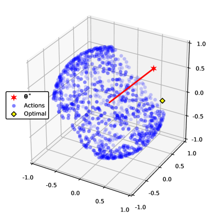
Figure 1: An example decision set in $\mathds{R}^{3}$ with $K=1000$ actions.

The rewards are either $-1$ or $+1$, with probabilities chosen so that $\mathds{E}[y_{t}]=\langle\bm{x}_{t},\bm{\theta}^{*}\rangle$. Therefore $\tilde{B}=1$ and, being bounded in the $[-1,1]$ interval, the reward distribution is subgaussian with $\sigma^{2}=1$.

The experiments below measure the expected regret in each case; the confidence parameter is $\alpha=1/n$, which is the usual choice when one wishes to minimize expected regret.

D.1 The Dependency of the Pseudo-Regret on the Dimension for Gap Instances

The first experiment was aimed at the open question of Section B.1, namely whether the gap-dependent regret is $\Omega(d^{2})$ in the dimension of the problem. Thus privacy wasn’t a concern in this particular setting; rather, our goal was to determine the performance of our general recipe algorithm in a contextual setting with a clear-cut gap. We measured the pseudo-regret of the non-private LinUCB algorithm as a function of the dimension over $n=10^{5}$ rounds with the regularizer $\rho=\bm{I}_{d\times d}$ and $K=d^{2}$ arms. The values of $d$ were logarithmically spaced in the interval $[4,64]$. The results of the experiment are plotted in Fig. 2. The two sub-experiments differ only in the reward noise distribution used. In the first, the reward noise is truly a Gaussian with $\sigma^{2}=1$, whereas in the second the reward is $\pm 1$ as described above (subgaussian with $\sigma^{2}=1$). In the latter case, the actual variance in the reward depends on its expectation, and is somewhat lower than 1. This is perhaps why the regret is somewhat lower than with gaussian reward noise.

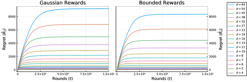
Figure 2: Experiment 1 — Regret over time for varying dimensions.

Figure 3 shows the same results with total accumulated regret plotted against dimension using a log–log scale. The best-fit line on this plot has a slope of roughly 2, clearly pointing to a super-linear dependency on $d$. We conjecture that, in general, the dependency on $d$ is indeed quadratic.

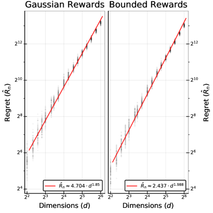
Figure 3: Experiment 1 — Regret vs. dimension with log–log axes and best-fit line.

D.2 Empirical Performance of the Privacy-Preserving Algorithms over Time

This experiment compares the expected regret of the various algorithm variants presented in this paper. The two major privacy-preserving algorithms are based on Wishart noise (Section 4.1) and Gaussian noise (Section 4.2); both were run with privacy parameters $\varepsilon=1.0$ and $\delta=0.1$ over a horizon of $n=5\times 10^{7}$ rounds and dimension $d=5$ and $K=d^{2}=25$. The results are shown in Fig. 4; the curves are truncated after $2\times 10^{7}$ rounds because they are essentially flat after this point.

The sub-figures of Fig. 4 show two settings that differ in the sub-optimality gap $\Delta$ between the rewards of the optimal and sub-optimal arms. In the left sub-figure, the algorithms are run in a setting without a structured gap ($\Delta=0$), where we have not forced all arms to be strictly separated from the optimal arm by a large reward gap. Here, all sub-optimal arms are distributed uniformly on the set $\{\bm{x}\in\mathds{R}^{d}\nonscript\>|\allowbreak\nonscript\>\mathopen{}\|\bm{x}\|=1,\langle\bm{x},\bm{\theta}^{*}\rangle\in[-0.75,0.75]\}$ (and not from $[-0.75,0.65]$ as in the previous experiment). Note that while we cannot guarantee that in all rounds there exists a gap between the optimal and sub-optimal arms, it is still true that in expectation we should observe a gap of $\Theta(\nicefrac{{1}}{{K}})$ between the optimal arm and the second-best arm (and as $K=25$ this expected gap is, still, a constant in comparison to $n$). In the right sub-figure, however, the sub-optimal arms are indeed separated by a gap of $\Delta=0.1$ from the optimal arms; their rewards lie in the interval $[-0.75,0.65]$ as in the previous experiment. In both cases there is always an optimal arm with reward $0.75$.

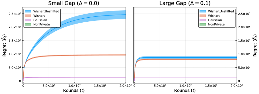
Figure 4: Experiment 2 — Regret over time, with and without forced sub-optimality gaps.

The figures show the following algorithm variants:

• The NonPrivate algorithm is LinUCB with regularizer $\rho=1.0$. Its regret is too small to be distinguished from the x-axis in this plot.

• The Gaussian variant is described in Section 4.2.

• The Wishart variant is described in Section 4.1 with the shift given in Eq. 4.

• The WishartUnshifted variant is that of Section 4.1 but with no shift.

Results.

It is apparent that, at least for this setting, the Gaussian noise algorithm outperforms Wishart noise. This shows that while the asymptotic performance of the two algorithms is fairly close, the constants in the Gaussian version of the algorithm are far better than the ones in the Wishart-noise based algorithm.

Furthermore, the performance of the WishartUnshifted variant changes significantly between the two cases — it has the worst regret in the no-gap setting ($\Delta=0$) but, surprisingly, it is statistically indistinguishable from the shifted Wishart variant in the large gap instance ($\Delta=0.1$). We investigate this relationship between the sub-optimality gap and shifted regularizers in the next experiment.

D.3 Empirical Performance of Shifted Regularizers for Different Suboptimality Gaps

In both the Wishart and Gaussian variants of our algorithm, we use a shifted regularization matrix $\bm{H}_{t}\pm c\bm{I}$, choosing the shift parameter $c$ to approximately optimize our regret bound in each case. This optimal shift parameter turns out not to depend on the sub-optimality gap $\Delta$ of the problem instance. The previous experiment showed, however, that in practice the relative performance of the shifted and unshifted Wishart variants changes drastically depending on the gap. In this experiment, we investigate the impact of varying the shift parameter for the Wishart and Gaussian mechanisms under different sub-optimality gaps $\Delta$.

All the parameters are the same as the previous experiment — the only difference is the shift parameter; the results are shown in Fig. 5. The two sub-figures show the performance of the Wishart and Gaussian variants, respectively. The x-axis is a logarithmic scale indicating $\rho_{\min}$, the high-probability lower bound on the minimum eigenvalue of the shifted regularizer matrix. $\rho_{\min}$ serves as a good proxy for the shift parameter because changing one has the effect of shifting the other by the same amount; it has the added benefit of being meaningfully comparable amongst the different algorithm variants. The vertical dotted lines indicate the $\rho_{\min}$ values corresponding to the algorithms from Sections 4.1 and 4.2 for the Wishart and Gaussian variants, respectively; these are also the algorithms examined in the previous experiment. The Gaussian mechanism does not have an unshifted variant.

Results.

Tuning the shift parameter appears to significantly affect the performance only for problem instances with relatively small or zero sub-optimality gaps. In the large-gap settings, on the other hand, having too much regularization does not seem to increase regret appreciably. The small-gap settings are exactly those in which exploration is crucial, so we conjecture that large regularizers inhibit exploration and thereby incur increased regret.

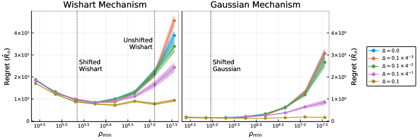
Figure 5: Experiment 3 — Varying shift parameters with different sub-optimality gaps.

References

• Abbasi-Yadkori et al. [2011] Yasin Abbasi-Yadkori, Dávid Pál, and Csaba Szepesvári. Improved algorithms for linear stochastic bandits. In J. Shawe-Taylor, R. S. Zemel, P. L. Bartlett, F. Pereira, and K. Q. Weinberger, editors, Advances in Neural Information Processing Systems, volume 24, pages 2312–2320. Curran Associates, Inc., 2011.
• Abbasi-Yadkori et al. [2012] Yasin Abbasi-Yadkori, Dávid Pál, and Csaba Szepesvári. Online-to-confidence-set conversions and application to sparse stochastic bandits. In AISTATS, pages 1–9, 2012.
• Abe et al. [2003] Naoki Abe, Alan W. Biermann, and Philip M. Long. Reinforcement learning with immediate rewards and linear hypotheses. Algorithmica, 37(4):263–293, 2003.
• Agrawal [1995] Rajeev Agrawal. Sample mean based index policies with O(log n) regret for the multi-armed bandit problem., volume 27, pages 1054–1078. Applied Probability Trust, 1995.
• Auer [2003] Peter Auer. Using confidence bounds for exploitation-exploration trade-offs. JMLR, 3:397–422, 2003.
• Auer et al. [2002] Peter Auer, Nicolò Cesa-Bianchi, and Paul Fischer. Finite-time analysis of the multiarmed bandit problem. JMLR, 47(2-3):235–256, 2002.
• Bassily et al. [2014] Raef Bassily, Adam Smith, and Abhradeep Thakurta. Private empirical risk minimization: Efficient algorithms and tight error bounds. In Proceedings of the 2014 IEEE 55th Annual Symposium on Foundations of Computer Science, FOCS ’14, pages 464–473, Washington, DC, USA, 2014. IEEE Computer Society. ISBN 978-1-4799-6517-5. doi: 10.1109/FOCS.2014.56.
• Berry and Fristedt [1985] Donald A Berry and Bert Fristedt. Bandit problems: sequential allocation of experiments. London ; New York : Chapman and Hall, 1985.
• Bun and Steinke [2016] Mark Bun and Thomas Steinke. Concentrated differential privacy: Simplifications, extensions, and lower bounds. In Theory of Cryptography, Lecture Notes in Computer Science, pages 635–658. Springer, Berlin, Heidelberg, November 2016. ISBN 978-3-662-53640-7 978-3-662-53641-4. doi: 10.1007/978-3-662-53641-4_24.
• Chan et al. [2010] T.-H. Hubert Chan, Elaine Shi, and Dawn Song. Private and continual release of statistics. In Automata, Languages and Programming, Lecture Notes in Computer Science, pages 405–417. Springer, Berlin, Heidelberg, July 2010. ISBN 978-3-642-14161-4 978-3-642-14162-1. doi: 10.1007/978-3-642-14162-1_34.
• Chaudhuri et al. [2011] Kamalika Chaudhuri, Claire Monteleoni, and Anand D. Sarwate. Differentially private empirical risk minimization. J. Mach. Learn. Res., 12:1069–1109, July 2011. ISSN 1532-4435.
• Chu et al. [2011] Wei Chu, Lihong Li, Lev Reyzin, and Robert E. Schapire. Contextual bandits with linear payoff functions. In AISTATS, volume 15 of JMLR Proceedings, pages 208–214, 2011.
• Dani et al. [2008] Varsha Dani, Thomas Hayes, and Sham Kakade. Stochastic linear optimization under bandit feedback. In 21st Annual Conference on Learning Theory, pages 355–366, January 2008.
• Dwork et al. [2010a] C. Dwork, G. N. Rothblum, and S. Vadhan. Boosting and differential privacy. In 2010 IEEE 51st Annual Symposium on Foundations of Computer Science, pages 51–60, October 2010a. doi: 10.1109/FOCS.2010.12.
• Dwork and Roth [2014] Cynthia Dwork and Aaron Roth. The algorithmic foundations of differential privacy. Foundations and Trends® in Theoretical Computer Science, 9(3–4):211–407, August 2014. ISSN 1551-305X, 1551-3068. doi: 10.1561/0400000042.
• Dwork et al. [2006a] Cynthia Dwork, Krishnaram Kenthapadi, Frank McSherry, Ilya Mironov, and Moni Naor. Our data, ourselves: Privacy via distributed noise generation. In Advances in Cryptology - EUROCRYPT 2006, Lecture Notes in Computer Science, pages 486–503. Springer, Berlin, Heidelberg, May 2006a. ISBN 978-3-540-34546-6 978-3-540-34547-3. doi: 10.1007/11761679_29.
• Dwork et al. [2006b] Cynthia Dwork, Frank McSherry, Kobbi Nissim, and Adam Smith. Calibrating noise to sensitivity in private data analysis. In Theory of Cryptography, Lecture Notes in Computer Science, pages 265–284. Springer, Berlin, Heidelberg, March 2006b. ISBN 978-3-540-32731-8 978-3-540-32732-5. doi: 10.1007/11681878_14.
• Dwork et al. [2010b] Cynthia Dwork, Moni Naor, Toniann Pitassi, and Guy N. Rothblum. Differential privacy under continual observation. In Proceedings of the Forty-Second ACM Symposium on Theory of Computing, STOC ’10, pages 715–724, New York, NY, USA, 2010b. ACM. ISBN 978-1-4503-0050-6. doi: 10.1145/1806689.1806787.
• Dwork et al. [2014] Cynthia Dwork, Kunal Talwar, Abhradeep Thakurta, and Li Zhang. Analyze Gauss: Optimal bounds for privacy-preserving principal component analysis. In Proceedings of the Forty-Sixth Annual ACM Symposium on Theory of Computing, STOC ’14, pages 11–20, New York, NY, USA, 2014. ACM. ISBN 978-1-4503-2710-7. doi: 10.1145/2591796.2591883.
• Hardt and Talwar [2010] Moritz Hardt and Kunal Talwar. On the geometry of differential privacy. In Proceedings of the Forty-Second ACM Symposium on Theory of Computing, STOC ’10, pages 705–714, New York, NY, USA, 2010. ACM. ISBN 978-1-4503-0050-6. doi: 10.1145/1806689.1806786.
• Jain et al. [2012] Prateek Jain, Pravesh Kothari, and Abhradeep Thakurta. Differentially private online learning. In Conference on Learning Theory, pages 24.1–24.34, June 2012.
• Karwa and Vadhan [2017] Vishesh Karwa and Salil Vadhan. Finite sample differentially private confidence intervals. arXiv:1711.03908 [cs, math, stat], November 2017.
• Kearns et al. [2014] Michael Kearns, Mallesh Pai, Aaron Roth, and Jonathan Ullman. Mechanism design in large games: Incentives and privacy. pages 403–410. ACM Press, 2014. ISBN 978-1-4503-2698-8. doi: 10.1145/2554797.2554834.
• Lattimore and Szepesvári [2017] Tor Lattimore and Csaba Szepesvári. The end of optimism? an asymptotic analysis of finite-armed linear bandits. In AISTATS, pages 728–737, 2017.
• Laurent and Massart [2000] B. Laurent and P. Massart. Adaptive estimation of a quadratic functional by model selection. The Annals of Statistics, 28(5):1302–1338, October 2000. ISSN 0090-5364, 2168-8966. doi: 10.1214/aos/1015957395.
• Mishra and Thakurta [2015] Nikita Mishra and Abhradeep Thakurta. (Nearly) optimal differentially private stochastic multi-arm bandits. In Proceedings of the Thirty-First Conference on Uncertainty in Artificial Intelligence, UAI’15, pages 592–601, Arlington, Virginia, United States, 2015. AUAI Press. ISBN 978-0-9966431-0-8.
• Neel and Roth [2018] Seth Neel and Aaron Roth. Mitigating bias in adaptive data gathering via differential privacy. In ICML, pages 3717–3726, 2018.
• Robbins [1952] Herbert Robbins. Some aspects of the sequential design of experiments. Bull. Amer. Math. Soc., 58(5):527–535, 09 1952.
• Rusmevichientong and Tsitsiklis [2010] Paat Rusmevichientong and John N. Tsitsiklis. Linearly parameterized bandits. Mathematics of Operations Research, 35(2):395–411, April 2010. ISSN 0364-765X. doi: 10.1287/moor.1100.0446.
• Sheffet [2015] Or Sheffet. Private approximations of the 2nd-moment matrix using existing techniques in linear regression. arXiv:1507.00056 [cs], June 2015.
• Smith and Thakurta [2013] Adam Smith and Abhradeep Thakurta. (Nearly) optimal algorithms for private online learning in full-information and bandit settings. In C. J. C. Burges, L. Bottou, M. Welling, Z. Ghahramani, and K. Q. Weinberger, editors, Advances in Neural Information Processing Systems 26, pages 2733–2741. Curran Associates, Inc., 2013.
• Tao [2012] Terence Tao. Topics in Random Matrix Theory, volume 132. American Mathematical Society Providence, RI, 2012.
• Tossou and Dimitrakakis [2016] Aristide C. Y. Tossou and Christos Dimitrakakis. Algorithms for differentially private multi-armed bandits. In Thirtieth AAAI Conference on Artificial Intelligence, March 2016.
• Tossou and Dimitrakakis [2017] Aristide C. Y. Tossou and Christos Dimitrakakis. Achieving privacy in the adversarial multi-armed bandit. arXiv:1701.04222 [cs], January 2017.
• Vershynin [2010] Roman Vershynin. Introduction to the non-asymptotic analysis of random matrices. arXiv:1011.3027 [cs, math], November 2010.
• Zhang [2011] Fuzhen Zhang. Matrix Theory: Basic Results and Techniques. Universitext. Springer, New York, 2nd edition, 2011. ISBN 978-1-4614-1098-0.