Structural nested mean models with irregularly spaced longitudinal observations

Abstract

Structural Nested Mean Models (SNMMs) are useful for causal inference of treatment effects in longitudinal observational studies. Most existing works assume that the data are collected at pre-fixed time points for all subjects, which, however, is restrictive in practice. To deal with irregularly spaced observations, we assume a class of continuous-time SNMMs and a martingale condition of no unmeasured confounding (NUC) to identify the causal parameters. We develop the first semiparametric efficiency theory and locally efficient estimators for continuous-time SNMMs. This task is non-trivial due to the restrictions from the NUC assumption imposed on the SNMM parameter. In the presence of dependent censoring, we propose an inverse probability of censoring weighting estimator, which achieves a multiple robustness feature in that it is unbiased if either the model for the treatment process or the potential outcome mean function is correctly specified, regardless whether the censoring model is correctly specified. The new framework allows us to conduct causal analysis respecting the underlying continuous-time nature of the data processes. We estimate the effect of time to initiate highly active antiretroviral therapy on the CD4 count at year 2 from the observational Acute Infection and Early Disease Research Program database.

Keywords: Causality; Counting process; Discretization; Multiple robustness; Martingale.

1 Introduction

1.1 Causal inference methods with time-varying confounding

The gold standard to draw causal inference of treatment effects is designing randomized experiments. However, randomized experiments are not always feasible due to practical constraints or ethical issues. Moreover, randomized experiments often have restrictive inclusion and exclusion criteria for patient enrollment, which limits the experiment results to be generalized to a larger real-world patient population. In these cases, observational studies are useful. In observational studies, confounding by indication poses a unique challenge to drawing valid causal inference of treatment effects. For example, sicker patients are more likely to take the active treatment, whereas healthier patients are more likely to take the control treatment. Consequently, it is not fair to compare the outcome from the treated group and the control group directly. Moreover, in longitudinal observational studies, confounding is likely to be time-dependent, in the sense that time-varying prognostic factors of the outcome affect the treatment assignment at each time, and thereby distort the association between treatment and outcome over time. In these cases, the traditional regression methods are biased even adjusting for the time-varying confounders (Robins et al., 1992, Hernán et al., 2000, 2005, Robins and Hernán, 2009, Orellana et al., 2010).

1.2 A motivating application

HAART (highly active antiretroviral therapy) is the standard of care as initial treatment for HIV. Our interest is motivated by the observational AIEDRP (Acute Infection and Early Disease Research Program) Core 01 study. This study established a cohort of HIV infected patients who have chosen to defer therapy but agree to be followed by this study. Deferring therapy may have an increased risk of permanent immune system damage but also a decreased risk of developing drug resistance. We aim to determine the effect of time to initiate HAART on disease progression for those patients who were diagnosed during acute or early HIV infection.

The outcome variable $Y$ is the CD4 count measured by the end of year $2$, for which lower counts indicate worse immunological function and disease progression. The inter-quantile range of the observed outcome in the AIEDRP database is from $443$ cells/mm³ to $794$ cells/mm³. In this database, $45\%$ of patients dropped out of the study before year 2, rendering $969$ patients with complete observations. Treatment initiation can only occur at follow-up visits and be determined by the discretion of physicians. By protocol, follow-up visits occur at weeks 2, 4, and 12, and then every 12 weeks thereafter, through week 96. However, as shown in Figure 1, both the number and the timings of visits differ from one patient to the next. Among all patients, $36\%$ of patients did not initiate the treatment before year 2. The observed time to treatment initiation ranges continuously from $12$ days to $282$ days. The covariates include age at infection, gender, race, injection drug ever/never, and measured CD4 count and log viral load at follow-up visits.

To answer the question of interest using the AIEDRP database, two major concerns arise: first, the association between the treatment and outcome processes, i.e., time-varying confounding, that would obscure the causal effect of time to treatment initiation on the CD4 outcome at year 2; second, the observations are irregularly spaced.

1.3 Structural nested mean models

Structural Nested Models (SNMs; Robins et al., 1992, Robins, 1994) have been proposed to overcome the challenges for causal inference with time-varying confounding. We focus on a class of SNMs for continuous outcomes, namely, structural nested mean models (SNMMs). We discuss the extension to accommodate the binary outcome and the survival outcome in Section 7. Most existing works on SNMMs assume discrete-time data generating processes and require all subjects to be followed at the same pre-fixed time points, such as months. The literature of discrete-time SNMMs is fruitful; see, e.g., Robins (1998b), Robins et al. (2000), Almirall et al. (2010), Chakraborty and Moodie (2013), Lok and DeGruttola (2012), Lok and Griner (2014), Yang and Lok (2016, 2018). However, as in the AIEDRP database, observational data are often collected by user-initiated visits to clinics, hospitals and pharmacies, and data are more likely to be measured at irregularly spaced time points, which are not necessarily the same for all subjects. Such data sources are now commonplace, such as electronic health records, claims databases, disease data registries, and so on (Chatterjee et al., 2016).

The existing causal framework does not directly apply in such situations, requiring some (possibly arbitrary) discretization of the timeline (Neugebauer et al., 2010). Such data pre-processing is quite standard and routine to practitioners, but leads to many unresolved problems: the treatment process depends transparently on the discretization, and therefore the interpretation of SNMMs depends on the definition of time interval (Robins, 1998a). Moreover, after discretization, the data may need to be recreated at certain time points. Consider monthly data for example. If a subject had multiple visits within the same month, a common strategy is to take the average of the multiple measures as the observation for a given variable at that month. If a subject had no visit for a given month, one may need to impute the missing observation. Because of such distortions, the resulting data may not satisfy the standard causal consistency or no unmeasured confounding (NUC) assumptions. Consequently, model parameters may not have a causal interpretation.

With irregularly spaced observations, it is more reasonable to assume that the data are generated from continuous-time processes. The work for causal models in continuous-time processes is somewhat sparse; exceptions include, e.g., Robins (1998a), Lok et al. (2004), Lok (2008), Zhang et al. (2011), Lok (2017). Extending the existing causal models with discrete-time processes to continuous-time processes is not trivial. An important challenge lies in time-dependent selection bias or confounding; e.g., in a health-related study, sicker patients may visit the doctor more frequently and are more likely to initiate the treatment. To overcome this challenge, following Lok (2008), we treat the observed treatment assignment process as a counting process $N_{T}(t)$ and assume a martingale condition of NUC on $N_{T}(t)$ to identify the SNMM parameters. Specifically, the NUC assumption entails that the jumping rate of $N_{T}(t)$ at $t$ does not depend on future potential outcomes, given the past treatment and covariate history up to $t$. A practical implication is that the covariate set should be rich enough to include all predictors of outcome and treatment, so that we can distinguish the treatment effect and the confounding effect. This assumption was also adopted in Zhang et al. (2011) and Yang et al. (2018) to the settings where the effect of a treatment varies in continuous time. Lok (2017) provided a strategy of constructing unbiased estimating equations exploiting the relationship between the mimicking potential outcome process and the treatment process, which leads to a large class of estimators. While this strategy provides unbiased estimators, there is no guidance on how to choose an efficient estimator, and a naive choice can lead to inaccurate estimation.

1.4 Semiparametric efficiency theory for continuous-time SNMMs

We establish the new semiparametric efficiency theory for continuous-time SNMMs with irregularly spaced observations. Toward this end, we follow the geometric approach of Bickel et al. (1993) for the semiparametric model by characterizing the nuisance tangent space, its orthogonal complementary space, and lastly the semiparametric efficiency score for the SNMM parameter.

In our problem, the SNMM and the NUC assumption constitute the semiparametric model for the data. Given the close relationship of causal inference and missing data theory, it is worthwhile to discuss the connection of the semiparametric efficiency development in our paper and that in the missing data literature (Ding and Li, 2018). The NUC assumption for the treatment process plays the same role of the ignorability assumption for the missing data mechanism; therefore, our characterization of the nuisance tangent space for the treatment process follows the same as that for the continuous-time missing data process; see Section 5.2 of Tsiatis (2006). Besides this analogy, our theoretical task is considerably more complicated. Although the NUC assumption does not have any testable implications on the observed-data likelihood (Van Der Laan and Dudoit, 2003, Tan, 2006), it imposes conditional independence restrictions on the treatment process and the counterfactual outcomes, given the past history, and hence restrictions for the SNMM parameter; see equation (9). To circumvent this complication, we use the variable transformation technique and translate the restrictions into the new variables, which leads to the unconstrained observed data-likelihood. This step allows us to characterize the semiparametric efficiency score for the SNMM parameter and construct locally efficient estimators which achieve the semiparametric efficiency bound.

In the AIEDRP database, a large portion of patients dropped out of the study before year 2. To accommodate possible dependent censoring due to drop-out, we propose the inverse probability of censoring weighting (IPCW) estimator. We show that the proposed estimator is multiply robust in that it is consistent if either the potential outcome mean model is correctly specified or the model for the treatment process is correctly specified, regardless whether the censoring model is correctly specified. This amounts to six scenarios specified in Table 1 that guarantee consistent estimation, allowing some components in the union of the three models to be misspecified (Molina et al., 2017, Wang and Tchetgen Tchetgen, 2018). Moreover, using the empirical process theory (van der Vaart and Wellner, 1996), we characterize the asymptotic property of the proposed estimator of the SNMM parameter under a parametric outcome mean model, and proportional hazards models for the treatment and censoring processes, allowing for multiply robust inference.

It is important to note that for regularly spaced observations, i.e. the data process can only take values at pre-fixed time points, the proposed estimator simplifies to the existing estimator with discrete-time data. For irregularly spaced observations, the new model and estimation framework allows us to deal with irregularly spaced observations directly and respects the nature of the underlying data generating mechanism. In contrast, the existing g-estimator requires data pre-processing and may introduce bias as demonstrated by simulation in Section 5.

The rest of the article is organized as follows. In Section 2, we describe the SNMM with discrete-time processes, which serves as a building block to establishing the semiparametric efficiency theory for continuous-time processes and also enables us to establish their connection. In Section 3, we present the semiparametric efficiency theory and locally efficient estimators for the continuous-time SNMM under the NUC assumption. Moreover, we propose an IPCW estimator to deal with dependent censoring due to premature dropout. In Section 4, we establish the asymptotic property of the estimator allowing for multiply robust inference. In Section 5, we present simulation studies to investigate the performance of the proposed estimator compared to the existing competitor in finite samples. In Section 6, we apply the proposed estimator to estimate the effect of the time between HIV infection and initiation of HAART on the CD4 count at year 2 after infection in HIV-positive patients with early and acute infection. We conclude the article with discussions in Section 7.

2 Structural nested mean models in discrete-time processes

2.1 Setup, models, and assumptions

We first describe the SNMM in discrete-time processes. We assume that $n$ subjects are followed at pre-fixed discrete times $t_{0}<\cdots<t_{K+1}$ with $t_{0}=0$ and $t_{K+1}=\tau$. We assume that the subjects are simple random samples from a larger population (Rubin, 1978). For simplicity, we suppress the subscript $i$ for subjects. Let $L_{m}$ be a vector of covariates at time $t_{m}$. Let $A_{m}$ be the treatment indicator at $t_{m}$; i.e., $A_{m}=1$ if the subject was on treatment at $t_{m}$ and $A_{m}=0$ otherwise. We use the overline notation to denote a variable’s history; e.g., $\overline{A}_{m}=(A_{0},\ldots,A_{m})$. We assume that once treatment is initiated, it is never discontinued, so each treatment regime corresponds to one treatment initiation time. Let $T$ be the time to treatment initiation, and let $T=\infty$ if the subject never initiated the treatment during the follow up. Let $\Gamma$ be the indicator that the treatment initiation time is less than $\tau$; i.e., $\Gamma=1$ if the subject initiated the treatment before $\tau$ and $\Gamma=0$ otherwise. Let $Y^{(m)}$ be the potential outcome at the end of study $\tau$, had the subject initiated the treatment at $t_{m}$, and let $Y^{(\infty)}$ be the potential outcome at $\tau$ had the subject never initiated the treatment during the study follow up. Let $V_{m}=(A_{m-1},L_{m})$ be the vector of treatment and covariate. Let $Y$ be the continuous outcome measured at $\tau$. Finally, the subject’s full record is $F=(\overline{A}_{K},\overline{L}_{K},Y)$.

Following Lok and DeGruttola (2012), we describe the discrete-time SNMM for the treatment effect as follows.

Assumption 1 (Discrete-time SNMM)

For $0\leq m\leq K$, the discrete-time SNMM is

$$\gamma_{m}(\overline{L}_{m})=\mathbb{E}\left\{Y^{(m)}-Y^{(\infty)}\mid\overline{A}_{m-1}=\overline{0},\overline{L}_{m}\right\}=\gamma_{m}(\overline{L}_{m};\psi^{*});$$ (1)

i.e., $\gamma_{m}(\overline{L}_{m};\psi)$ with $\psi\in$$\mathbb{R}^{p}$ is a correctly specified model for $\gamma_{m}(\overline{L}_{m})$ with the true parameter value $\psi^{*}.$

This model specifies the conditional expectation of the treatment contrasts $Y^{(m)}-Y^{(\infty)}$, given subject’s observed treatment and covariates history $(\overline{A}_{m-1}=\overline{0},\overline{L}_{m})$. Intuitively, it states that the conditional mean of the outcome is shifted by $\gamma_{m}(\overline{L}_{m};\psi^{*})$ had the subject initiated the treatment at $t_{m}$ comparing to never starting. Therefore, the parameter $\psi^{*}$ has a causal interpretation. To help understand the model, consider $\gamma_{m}(\overline{L}_{m};\psi^{*})=(\psi_{1}^{*}+\psi_{2}^{*}t_{m})(\tau-t_{m})$, where $\psi^{*}=(\psi_{1}^{*},\psi_{2}^{*})$. This model entails that on average, the treatment would increase the mean of the outcome had the subject initiated the treatment at $t_{m}$ by $(\psi_{1}^{*}+\psi_{2}^{*}t_{m})(\tau-t_{m})$, and the magnitude of the increase depends on the duration of the treatment and the treatment initiation time. If $\psi_{1}^{*}+\psi_{2}^{*}t_{m}>0$ and $\psi_{2}^{*}<0$, it indicates the treatment is beneficial and earlier initiation is better.

We make the consistency assumption to link the observed data to the potential outcomes.

Assumption 2 (Consistency)

The observed outcome is equal to the potential outcome under the actual treatment received; i.e., $Y=Y^{(T)}$.

If all potential outcomes were observed for each subject, we can directly compare these outcomes to infer the treatment effect; however, the fundamental problem in causal inference is that we can not observe all potential outcomes for a particular subject (Holland, 1986). In particular, we can observe $Y^{(\infty)}$ only for the subjects who did not initiate the treatment during the follow up. To overcome this issue, we define

$$H(\psi^{*})=Y-\gamma_{T}(\overline{L}_{T};\psi^{*}).$$ (2)

Intuitively, $H(\psi^{*})$ subtracts the treatment effect $\gamma_{T}(\overline{L}_{T};\psi^{*})$ from the observed outcome $Y$, so it mimics the potential outcome $Y^{(\infty)}$ had the treatment never been initiated. We provide the formal statement as proved in Lok and DeGruttola (2012).

Proposition 1 (Mimicking $Y^{(\infty)}$)

Under Assumption 2, $H(\psi^{*})$ mimics $Y^{(\infty)}$, in the sense that

$$\mathbb{E}\left\{H(\psi^{*})\mid\overline{A}_{m-1}=\overline{0},A_{m},\overline{L}_{m}\right\}=\mathbb{E}\left\{Y^{(\infty)}\mid\overline{A}_{m-1}=\overline{0},A_{m},\overline{L}_{m}\right\},$$

for $0\leq m\leq K,$ where by convention, $\mathbb{E}\left(\cdot\mid\overline{A}_{-1}=\overline{0},A_{0},\overline{L}_{0}\right)=\mathbb{E}\left(\cdot\mid A_{0},\overline{L}_{0}\right)$.

We can not fit the SNMM by a regression model pooled over time, because the model involves the unobserved potential outcomes. Parameter identification requires the NUC assumption (Robins et al., 1992).

Assumption 3 (No unmeasured confounding)

$A_{m}\mathbin{\mathchoice{\hbox to0.0pt{\hbox{$\displaystyle\perp$}\hss}\kern 3.46875pt{}\kern 3.46875pt\hbox{$\displaystyle\perp$}}{\hbox to0.0pt{\hbox{$\textstyle\perp$}\hss}\kern 3.46875pt{}\kern 3.46875pt\hbox{$\textstyle\perp$}}{\hbox to0.0pt{\hbox{$\scriptstyle\perp$}\hss}\kern 2.36812pt{}\kern 2.36812pt\hbox{$\scriptstyle\perp$}}{\hbox to0.0pt{\hbox{$\scriptscriptstyle\perp$}\hss}\kern 1.63437pt{}\kern 1.63437pt\hbox{$\scriptscriptstyle\perp$}}}Y^{(\infty)}\mid(\overline{A}_{m-1},\overline{L}_{m})$ for $0\leq m\leq K$, where $\mathbin{\mathchoice{\hbox to0.0pt{\hbox{$\displaystyle\perp$}\hss}\kern 3.46875pt{}\kern 3.46875pt\hbox{$\displaystyle\perp$}}{\hbox to0.0pt{\hbox{$\textstyle\perp$}\hss}\kern 3.46875pt{}\kern 3.46875pt\hbox{$\textstyle\perp$}}{\hbox to0.0pt{\hbox{$\scriptstyle\perp$}\hss}\kern 2.36812pt{}\kern 2.36812pt\hbox{$\scriptstyle\perp$}}{\hbox to0.0pt{\hbox{$\scriptscriptstyle\perp$}\hss}\kern 1.63437pt{}\kern 1.63437pt\hbox{$\scriptscriptstyle\perp$}}}$ means “is (conditionally) independent of” (Dawid, 1979).

Assumption 3 holds if $(\overline{A}_{m-1},\overline{L}_{m})$ contains all prognostic factors for $Y^{(\infty)}$ that affect the treatment decision at $t_{m}$ for $0\leq m\leq K$. Under this assumption, the observational study can be conceptualized as a sequentially randomized experiment.

Proposition 1 implies that under Assumption 3, for $0\leq m\leq K$,

$$\mathbb{E}\left\{H(\psi^{*})\mid\overline{A}_{m-1}=\overline{0},A_{m},\overline{L}_{m}\right\}=\mathbb{E}\left\{H(\psi^{*})\mid\overline{A}_{m-1}=\overline{0},\overline{L}_{m}\right\};$$ (3)

see, e.g., Robins et al. (1992), Lok et al. (2004), Lok and DeGruttola (2012). Equation (3) also poses restrictions for $\psi^{*}$.

2.2 Semiparametric efficiency theory

The semiparametric model is characterized by the discrete-time SNMM (1) and restriction (3), where the parameter of primary interest is $\psi^{*}$.

We first present the general semiparametric efficiency theory. Suppose the data consist of $n$ independent and identically distributed random variables $F_{1},\ldots,F_{n}$. We consider regular asymptotically linear (RAL) estimators $\widehat{\psi}_{n}$ for $\psi^{*}$ as

$$n^{1/2}(\widehat{\psi}_{n}-\psi^{*})=n^{1/2}\mathbb{P}_{n}\Phi(F)+o_{p}(1),$$ (4)

where $\mathbb{P}_{n}$ denotes the empirical mean; i.e., $\mathbb{P}_{n}\Phi(F)=n^{-1}\sum_{i=1}^{n}\Phi(F_{i})$, $\Phi(F)$ is called the influence function of $\widehat{\psi}_{n}$, with mean zero and finite and non-singular variance. Because $\psi^{*}$ is $p$-dimensional, $\Phi(F)$ is also $p$-dimensional. From (4), the asymptotic variance of $n^{1/2}(\widehat{\psi}_{n}-\psi^{*})$ is equal to the variance of its influence function. As a result, to construct the efficient RAL estimator, it suffices to find the influence function with the smallest variance.

To do this, we take a geometric approach of Bickel et al. (1993). Consider the Hilbert space $\mathcal{H}$ of all $p$-dimensional, mean-zero finite variance measurable functions of $F$, denoted by $h(F)$, equipped with the covariance inner product $<h_{1},h_{2}>=\mathbb{E}\left\{h_{1}(F)^{\mathrm{\scriptscriptstyle T}}h_{2}(F)\right\}$ and the norm $||h||=\mathbb{E}\left\{h(F)^{\mathrm{\scriptscriptstyle T}}h(F)\right\}^{1/2}<\infty$. Bickel et al. (1993) stated that influence functions for RAL estimators lie in the orthogonal complement of the nuisance tangent space in $\mathcal{H}$. To motive the concept of the nuisance tangent space for a semiparametric model, we first consider a fully parametric model $f(F;\psi,\theta)$, where $\psi$ is a $p$-dimensional parameter of interest, and $\theta$ is an $q$-dimensional nuisance parameter. The score vectors of $\psi$ and $\theta$ are $S_{\psi}(F)=\partial\log f(F;\psi,\theta^{*})/\partial\psi$ and $S_{\theta}(F)=\partial\log f(F;\psi^{*},\theta)/\partial\theta$, both evaluated at the true values $(\psi^{*},\theta^{*})$, respectively. For a parametric model, the nuisance tangent space $\Lambda$ is the linear space in $\mathcal{H}$ spanned by the $q$-dimensional nuisance score vector $S_{\theta}(F)$. For semiparametric models, where the nuisance parameter is infinite-dimensional, the nuisance tangent space $\Lambda$ is defined as the mean squared closure of all parametric sub-model nuisance tangent spaces. The efficient score $S_{\mathrm{eff}}(F)$ for the semiparametric model is the projection of $S_{\psi}$ onto the orthogonal complementary space of the nuisance tangent space $\Lambda^{\bot}$; i.e., $S_{\mathrm{eff}}(F)=\prod\left(S_{\psi}\mid\Lambda^{\bot}\right)$, where $\prod$ is the projection operator in the Hilbert space. The efficient influence function is $\Phi_{\mathrm{eff}}(F)=\left[\mathbb{E}\left\{S_{\mathrm{eff}}(F)S_{\mathrm{eff}}(F)^{\mathrm{\scriptscriptstyle T}}\right\}\right]^{-1}S_{\mathrm{eff}}(F)$, with the variance $\left[\mathbb{E}\left\{S_{\mathrm{eff}}(F)S_{\mathrm{eff}}(F)^{\mathrm{\scriptscriptstyle T}}\right\}\right]^{-1}$, which achieves the semiparametric efficiency bound (Bickel et al., 1993). From this geometric point of view, to derive efficient semiparametric estimators for $\psi^{*}$, it suffices to find the efficient score $S_{\mathrm{eff}}(F)$.

2.3 Influence functions

The key step is to characterize the space where the influence functions of RAL estimators belong to, i.e., the orthogonal complementary space of the nuisance tangent space $\Lambda^{\bot}$. Following Robins (1994), Proposition 2 characterizes all influence functions of RAL estimators for $\psi^{*}$.

Proposition 2

For the semiparametric model characterized by the discrete-time SNMM (1) and restriction (3), the influence function space for $\psi^{*}$ is

$$\Lambda^{\bot}=\left\{G(\psi^{*};F,c):\ \text{for all }c(\overline{V}_{m})\in\mathbb{\mathbb{R}}^{p}\right\},$$ (5)

where $\overline{V}_{m}=(\overline{A}_{m-1},\overline{L}_{m})$ and

$$G(\psi;F,c)=\sum_{m=1}^{K}c(\overline{V}_{m})\{A_{m}-{P}(A_{m}=1\mid\overline{V}_{m})\}[H(\psi)-\mathbb{E}\{H(\psi)\mid\overline{V}_{m}\}],$$

indexed by $c$. To make the notation accurate, the abbreviation $c$ in $G(\psi;F,c)$ means $c(\overline{V}_{m})$.

Although Robins (1994) provided this result, the technical proofs were dense and less accessible to general readers. In the future, we will write a technical report that provides details to guide general readers in deriving the semiparametric efficiency theory in similar contexts.

The semiparametric efficiency score, i.e. the most efficient one among the class in (5), often does not have a closed-form expression. We now make a working assumption, which extends restriction (3) and allows us to derive an analytical expression of the semiparametric efficient score of $\psi^{*}.$

Assumption 4 (Homoscedasticity)

For $0\leq m\leq K$, $\mathrm{var}\{H(\psi^{*})\mid\overline{A}_{m},\overline{L}_{m}\}=\mathrm{var}\left\{H(\psi^{*})\mid\overline{V}_{m}\right\}$.

Proposition 3 (Discrete-time semiparametric efficient score)

Consider $\gamma_{m}(\overline{L}_{m};\psi^{*})=(\psi_{1}^{*}+\psi_{2}^{*}t_{m})(\tau-t_{m})$. Suppose Assumptions 2–4 holds. The semiparametric efficient score of $\psi^{*}$ is

$$S_{\mathrm{eff}}(\psi^{*};F)=G(\psi^{*};F,c_{\mathrm{eff}}),$$ (6)

where

$$c_{\mathrm{eff}}(\overline{V}_{m})=\left(\begin{array}[]{c}(\tau-t_{m})-\mathbb{E}\left\{\mathrm{dur}(t_{m})\mid\overline{A}_{m}=\overline{0},\overline{L}_{m}\right\}\\ t_{m}(\tau-t_{m})-\mathbb{E}\left\{T\times\mathrm{dur}(t_{m})\mid\overline{A}_{m}=\overline{0},\overline{L}_{m}\right\}\end{array}\right)\left[\mathrm{var}\left\{H(\psi^{*})\mid\overline{V}_{m}\right\}\right]^{-1},$$

and $\mathrm{dur}(t_{m})=\sum_{l=m}^{K-1}A_{l}(t_{l+1}-t_{l})$ is the observed treatment duration from $t_{m}$ to $\tau$.

3 SNMMs in continuous-time processes

3.1 Setup, models, and assumptions

We now extend the discrete-time SNMM in Section 2 to the continuous-time SNMM. We assume that the variables can change their values at any real time between $0$ and $\tau$. We assume that all subjects are followed until $\tau$ and consider censoring in Section 3.4.

Each subject has multiple visit times. Let $N(t)$ be the counting process for the visit times. Let $L_{t}$ be the multidimensional covariate process. In contrast to the setting with discrete-time data processes, $L_{t}$ is a vector of covariates at $t$ and additional information of the past visit times up to but not including $t$. This is because the past visit pattern, e.g., the number and frequency of the visit times may be important confounders for the treatment and outcome processes. Let $A_{t}$ be the binary treatment process. In our motivating application, the treatment can only be initiated at the follow-up visits; i.e., if $A_{t}=1$, then $N(t)=1$. We will model the treatment process directly, although one can model first the visit time process and then treatment assignment at the visit times. Define $Y^{(t)}$ as the potential outcome at $\tau$ had the subject initiated the treatment at $t$, and define $Y^{(\infty)}$ as the potential outcome at $\tau$ had the subject never initiated the treatment before $\tau$. Let $Y$ be the continuous outcome measured at $\tau$. For the regularization purpose, we assume that the processes are Càdlàg processes, i.e., the processes are right continuous with left limits. Let $V_{t}=(A_{t-},L_{t})$ be the combined treatment and covariate process, where $A_{t-}$ is the available treatment information right before $t$. We use the overline notation to denote a variable’s observed history; e.g., $\overline{A}_{t}=\{A_{u}:0\leq u\leq t,\mathrm{d}N(u)=1\}$. The subject’s full record is $F=\{\overline{V}_{\tau},(Y^{(t)}:0\leq t\leq\tau)\}.$ The observed data for a subject through $\tau$ is $O=(\overline{V}_{\tau},Y)$.

We assume the continuous-time SNMM as follows.

Assumption 5 (Continuous-time SNMM)

For $0\leq t\leq\tau$, the continuous-time SNMM is

$$\gamma_{t}(\overline{L}_{t})=\mathbb{E}\left\{Y^{(t)}-Y^{(\infty)}\mid\overline{L}_{t},T\geq t\right\}=\gamma_{t}(\overline{L}_{t};\psi^{*});$$ (7)

i.e., $\gamma_{t}(\overline{L}_{t};\psi)$ with $\psi\in$$\mathbb{R}^{p}$ is a correctly specified model for $\gamma_{t}(\overline{L}_{t})$ with the true parameter value $\psi^{*}.$ Moreover, $Y^{(t)}\sim Y^{(\infty)}+\gamma_{t}(\overline{L}_{t};\psi^{*})$ given $(\overline{L}_{t},T\geq t)$, where $\sim$ means “is (conditionally) distributed as”.

In the continuous-time SNMM (7), $\psi^{*}$ can be interpreted as the treatment effect rate for the outcome. For the continuous-time SNMM, we assume that given $(\overline{L}_{t},T\geq t)$, the treatment effect only changes the location of the distribution of the outcome but not on other aspects of the distribution such as the variance. This assumption is stronger than the discrete-time SNMM in Assumption 1. But this assumption is weaker than the rank-preserving assumption of $Y^{(t)}=Y^{(\infty)}+\gamma_{t}(\overline{L}_{t};\psi^{*})$ considered in Zhang et al. (2011). It has been argued that by mapping the potential outcomes directly rather than between distributions, rank preserving models are easier to understand and communicate (Vansteelandt et al., 2014). However, the rank preservation may be restrictive in practice, because it implies that for two subjects $i$ and $j$ with the same treatment and covariate history, $Y_{i}>Y_{j}$ must imply $Y_{i}^{(\infty)}>Y_{j}^{(\infty)}$. We relax this restriction by imposing a distributional assumption.

The continuous-time SNMM (7) can model the treatment effect flexibly. For example, the two-parameter model $\gamma_{t}(\overline{L}_{t};\psi^{*})=(\psi_{1}^{*}+\psi_{2}^{*}t)(\tau-t)I(t\leq\tau)$ entails that the treatment effect depends on the treatment initiation time and the duration of the treatment. To allow for treatment effect modifiers, we can specify an elaborated treatment effect model including time-varying covariates, such as viral load in the blood. For example, one can consider $\gamma_{t}(\overline{L}_{t};\psi^{*})=(\psi_{1}^{*}+\psi_{2}^{*}t+\psi_{3}^{*}\text{lvl}_{t})(\tau-t)I(t\leq\tau)$, where lvl_t is the log viral load at $t$. We discuss effect modification and model selection in Section 7.

To link the observed outcome to the potential outcomes, we assume that $Y=Y^{(T)}$. Define the mimicking outcome for $Y^{(\infty)}$ as $H(\psi^{*})=Y-\gamma_{T}(\overline{L}_{T};\psi^{*})$. By Assumption 5, $H(\psi^{*})\sim Y^{(\infty)},$ given $(\overline{L}_{t},T\geq t)$.

An important issue with data from user-initiated visits and treatment initiation is the potential selection bias and confounding, e.g., sicker patients may visit the doctor more frequently and are likely to initiate treatment earlier. To overcome this issue, we impose the NUC assumption on the treatment process (Yang et al., 2018).

Assumption 6 (No unmeasured confounding)

The hazard of treatment initiation is

$$\lambda_{T}(t\mid F) = \lim_{h\rightarrow 0}h^{-1}P(t\leq T<t+h,\Gamma=1\mid\overline{V}_{t},T\geq t,Y^{(\infty)})$$ (8)

$$= \lim_{h\rightarrow 0}h^{-1}P(t\leq T<t+h,\Gamma=1\mid\overline{V}_{t},T\geq t)=\lambda_{T}\left(t\mid\overline{V}_{t}\right).$$

Assumption 6 implies that the hazard of treatment initiation at $t$ depends only on the observed treatment and covariate history $\overline{V}_{t}$ but not on the future observations and potential outcomes. This assumption holds if the set of historical covariates contains all prognostic factors for the outcome that affect the decision of patient visiting the doctor and initiating treatment. As an example, in the motivating application, time-invariant characteristics such as age at infection, gender, race and whether ever used injection drugs are important confounders for the treatment and outcome processes. Moreover, time-varying CD4 and viral load are important confounders. Often, poor disease progression necessitates more frequent follow-up visits and earlier treatment initiation.

The treatment process $A_{t}$ can also be represented in terms of the counting process $N_{T}(t)$ and the at-risk process $Y_{T}(t)$ of observing treatment initiation. Let $\sigma(V_{t})$ be the $\sigma$-field generated by $V_{t}$, and let $\sigma(\overline{V}_{t})$ be the $\sigma$-field generated by $\cup_{u\leq t}\sigma(V_{u})$. Under the standard regularity conditions for the counting process, $M_{T}(t)=N_{T}(t)-\int_{0}^{t}\lambda_{T}(u\mid\overline{V}_{u})Y_{T}(u)\mathrm{d}u$ is a martingale with respect to the filtration $\sigma(\overline{V}_{t})$. Assumption 6 entails that the jumping rate of $N_{T}(t)$ at $t$ does not depend on $Y^{(\infty)}$, given $\overline{V}_{t}$. Because $H(\psi^{*})$ mimics $Y^{(\infty)}$ in the sense that it has the same distribution as $Y^{(\infty)}$ given $\overline{V}_{t}$, Assumption 6 also implies that the jumping rate of $N_{T}(t)$ at $t$ does not depend on $H(\psi^{*})$, given $\overline{V}_{t}$. To be formal, we show in the supplementary material that

$$\lambda_{T}\{t\mid\overline{V}_{t},H(\psi^{*})\}=\lambda_{T}(t\mid\overline{V}_{t}).$$ (9)

Therefore, under the standard regularity conditions, $M_{T}(t)$ is a martingale with respect to the filtration $\sigma\{\overline{V}_{t},H(\psi^{*})\}$. Lok (2008) imposed this martingale condition to formulate the NUC assumption for the treatment process.

3.2 Semiparametric efficiency score

To estimate the causal parameter precisely, we establish the new semiparametric efficiency theory for the continuous-time SNMMs. We defer all proofs to the supplementary material.

Theorem 1

For the semiparametric model characterized by the continuous-time SNMM (7) and Assumption 6, the influence function space for $\psi^{*}$ is

$$\Lambda^{\bot}=\left\{G(\psi^{*};F,c):\ \text{for all }c(\overline{V}_{u})\in\mathbb{\mathbb{R}}^{p}\right\},$$

where

$$G(\psi;F,c)=\int_{0}^{\tau}c(\overline{V}_{u})\left[H(\psi)-\mathbb{E}\left\{H(\psi)\mid\overline{V}_{u},T\geq u\right\}\right]Y_{T}(u)\mathrm{d}M_{T}(u).$$ (10)

The semiparametric efficiency score for $\psi^{*}$ is $S_{\mathrm{eff}}(\psi^{*};F)=\prod\{S(\psi^{*};F)\mid\Lambda^{\bot}\}$. To derive $S_{\mathrm{eff}}(\psi^{*};F)$, we calculate the projection of any $B=B(F)$ onto $\Lambda^{\bot}.$

Theorem 2

For any $B=B(F)$, the projection of $B$ onto $\Lambda^{\bot}$ is

$$\prod\left(B\mid\Lambda^{\bot}\right)=\int_{0}^{\tau}\left[\mathbb{E}\left\{B\dot{H}_{u}(\psi^{*})\mid\overline{V}_{u},T=u\right\}-\mathbb{E}\left\{B\dot{H}_{u}(\psi^{*})\mid\overline{V}_{u},T\geq u\right\}\right]\\ \times\left[\mathrm{var}\left\{H(\psi^{*})\mid\overline{V}_{u},T\geq u\right\}\right]^{-1}\left[H(\psi^{*})-\mathbb{E}\left\{H(\psi^{*})\mid\overline{V}_{u},T\geq u\right\}\right]\mathrm{d}M_{T}(u),$$ (11)

where $\dot{H}_{u}(\psi^{*})=H(\psi^{*})-\mathbb{E}\{H(\psi^{*})\mid\overline{V}_{u},T\geq u\}$.

Considering $B=S(\psi^{*};F)$ in Theorem 2, we can derive the semiparametric efficient score for $\psi^{*}$.

Theorem 3 (Continuous-time semiparametric efficient score)

For the semiparametric model characterized by the continuous-time SNMM (7) and Assumption 6, the semiparametric efficient score of $\psi^{*}$ is

$$S_{\mathrm{eff}}(\psi^{*};F)=G(\psi^{*};F,c_{\mathrm{eff}}),$$ (12)

where $G(\psi;F,c)$ is defined in (10), and

$$c_{\mathrm{eff}}(\overline{V}_{u})=[\mathbb{E}\{\partial\dot{H}_{u}(\psi^{*})/\partial\psi\mid\overline{V}_{u},T=u\}\\ -\mathbb{E}\{\partial\dot{H}_{u}(\psi^{*})/\partial\psi\mid\overline{V}_{u},T\geq u\}]\times[\mathrm{var}\{H(\psi^{*})\mid\overline{V}_{u},T\geq u\}]^{-1}.$$ (13)

To illustrate the theorem, we provide the explicit expression of the semiparametric efficient score using an example.

Example 1

Consider $\gamma_{t}(\overline{L}_{t};\psi)=(\psi_{1}+\psi_{2}t)(\tau-t)I(t\leq\tau)$. Suppose Assumption 6 holds. The semiparametric efficient score of $\psi^{*}$ is $S_{\mathrm{eff}}(\psi^{*};F)=G(\psi^{*};F,c_{\mathrm{eff}})$, where

$$c_{\mathrm{eff}}(\overline{V}_{u})=\left(\begin{array}[]{c}(\tau-u)I(u\leq\tau)-\mathbb{E}\{(\tau-T)I(T\leq\tau)\mid\overline{V}_{u},T\geq u\}\\ u(\tau-u)I(u\leq\tau)-\mathbb{E}\{T(\tau-T)I(T\leq\tau)\mid\overline{V}_{u},T\geq u\}\end{array}\right)\\ \times[\mathrm{var}\{H(\psi^{*})\mid\overline{V}_{u},T\geq u\}]^{-1}.$$ (14)

Remark 1

The proposed continuous-time semiparametric efficient score contains the discrete-time semiparametric efficient score as a special case. If the processes take observations at discrete times $\{t_{0},\ldots,t_{K}\}$, then (i) the conditioning event $(\overline{V}_{u},T\geq u)$ at $t_{m}$ is the same as $(\overline{A}_{m}=\overline{0},\overline{L}_{m})$, (ii) $M_{T}(t)=N_{T}(t)-\int_{0}^{t}\lambda_{T}(u\mid\overline{V}_{u})Y_{T}(u)\mathrm{d}u$ at $t=t_{m}$ becomes $A_{m}-{P}(A_{m}=1\mid\overline{A}_{m-1}=\overline{0},\overline{L}_{m})$, and $\mathbb{E}\{\partial\dot{H}_{t}(\psi^{*})/\partial\psi\mid\overline{V}_{t},T=t\}$ at $t=t_{m}$ becomes

$$\mathbb{E}\{\partial\dot{H}_{m}(\psi^{*})/\partial\psi\mid\overline{V}_{m},T=t_{m}\}=-\left(\begin{array}[]{c}(\tau-t_{m})-\mathbb{E}\left\{\mathrm{dur}(t_{m})\mid\overline{A}_{m}=\overline{0},\overline{L}_{m}\right\}\\ t_{m}(\tau-t_{m})-\mathbb{E}\left\{T\times\mathrm{dur}(t_{m})\mid\overline{A}_{m}=\overline{0},\overline{L}_{m}\right\}\end{array}\right).$$

Therefore, the continuous-time semiparametric efficient score (12) reduces to the discrete-time semiparametric efficient score (6).

3.3 Doubly robust and locally efficient estimators

We now construct a general class of estimators based on the estimating function $G(\psi^{*};F,c)$. Because $\mathbb{E}\{G(\psi^{*};F,c)\}=0$, we obtain the estimator of $\psi^{*}$ by solving

$$\mathbb{P}_{n}\left\{G(\psi;F,c)\right\}=0.$$ (15)

In particular, the estimating equation (15) with $c_{\mathrm{eff}}$ provides the semiparametric efficient estimator of $\psi^{*}$.

In (15), we assume that the model for the treatment process and $\mathbb{E}\left\{H(\psi^{*})\mid\overline{V}_{u},T\geq u\right\}$ are known. In practice, they are often unknown and must be modeled and estimated from the data. We posit a proportional hazards model with time-dependent covariates for the treatment process; i.e.,

$$\lambda_{T}\left(t\mid\overline{V}_{t};\alpha\right) = \lambda_{T,0}(t)\exp\left\{\alpha^{\mathrm{\scriptscriptstyle T}}W_{T}(t,\overline{V}_{t})\right\},$$ (16)

where $\lambda_{T,0}(t)$ is an unknown baseline hazard function, $W_{T}(t,\overline{V}_{t})$ is a pre-specified function of $t$ and $\overline{V}_{t}$, and $\alpha$ is a vector of unknown parameters. Under Assumption 6, we can estimate $\lambda_{T,0}(t)$ and $\alpha$ from the standard software such as “coxph” in R (R Development Core Team, 2012) . To estimate $\alpha$, fit the time-dependent proportional hazards model to the data $\{(\overline{V}_{T_{i},i},T_{i},\Gamma_{i}):i=1,\ldots,n\}$ treating the treatment initiation as the failure event. Once we obtain $\widehat{\alpha},$ we can estimate the cumulative baseline hazard, $\lambda_{T,0}(t)\mathrm{d}t$ by

$$\widehat{\lambda}_{T,0}(t)\mathrm{d}t=\frac{\sum_{i=1}^{n}\mathrm{d}N_{T,i}(t)}{\sum_{i=1}^{n}\exp\left\{\widehat{\alpha}^{\mathrm{\scriptscriptstyle T}}W_{T}(t,\overline{V}_{t,i})\right\}Y_{T_{i}}(t)}.$$

Then, we obtain $\widehat{\lambda}_{T}(u\mid\overline{V}_{u})=\exp\left\{\widehat{\alpha}^{\mathrm{\scriptscriptstyle T}}W_{T}(u,\overline{V}_{u})\right\}\widehat{\lambda}_{T,0}(u)$ and $\widehat{M}_{T}(t)=N_{T}(t)-\int_{0}^{t}\widehat{\lambda}_{T}(u\mid\overline{V}_{u})Y_{T}(u)\mathrm{d}u$.

We also posit a working model $\mathbb{E}\left\{H(\psi^{*})\mid\overline{V}_{u},T\geq u;\beta\right\}$, such as a linear regression model, where $\beta$ is a vector of unknown parameters.

The estimating equation for $\psi^{*}$ achieves the double robustness or double protection (Rotnitzky and Vansteelandt, 2015).

Theorem 4 (Double robustness)

Under the continuous-time SNMM (7) and Assumption 6, the proposed estimator $\widehat{\psi}$ solving the estimating equation (15) is doubly robust in that it is unbiased if either the model for the treatment process is correctly specified, or the potential outcome mean model $\mathbb{E}\left\{H(\psi^{*})\mid\overline{V}_{u},T\geq u;\beta\right\}$ is correctly specified, but not necessarily both.

The choice of $c$ does not affect the double robustness but the efficiency of the resulting estimator. For efficiency consideration, we consider $c_{\mathrm{eff}}$ in (13). The resulting estimator solving the estimating equation (15) with $c_{\mathrm{eff}}$ is locally efficient, in the sense that it achieves the semiparametric efficiency bound if the working models for the treatment process and the potential outcome mean are correctly specified. Because $c_{\mathrm{eff}}$ depends on the unknown distribution, we require additional models for $\mathbb{E}\{(\tau-T)I(T\leq\tau)\mid\overline{V}_{u},T\geq u\}$ and $\mathbb{E}\{T(\tau-T)I(T\leq\tau)\mid\overline{V}_{u},T\geq u\}$ to approximate $c_{\mathrm{eff}}.$ For example, we can approximate $\mathbb{E}\{(\tau-T)I(T\leq\tau)\mid\overline{V}_{u},T\geq u\}$ by $P(T\leq\tau\mid\overline{V}_{u},T\geq u)\times\mathbb{E}\{\tau-T\mid\overline{V}_{u},u\leq T\leq\tau\}$ and each approximated by (logistic) linear models. For $\mathrm{\mathrm{var}}\{H(\psi^{*})\mid\overline{V}_{u},T\geq u\}$, we consider the following options: (i) assume $\mathrm{var}\{H(\psi^{*})\mid\overline{V}_{u},T\geq u\}$ to be a constant, and (ii) approximate $\mathrm{var}\{H(\psi^{*})\mid\overline{V}_{u},T\geq u\}$ by the sample variance of $H(\widehat{\psi}_{p})$ among subjects with $T\geq u$, where $\widehat{\psi}_{p}$ is a preliminary estimator. We compare the two options via simulation. Although option (ii) provides a slight efficiency gain in estimation, for ease of implementation we recommend option (i). Option (i) is common in the generalized estimating equation framework. From here on, we use this option for $c$ and suppress the dependence on $c$ for estimating functions.

3.4 Censoring

As in the AIEDRP study, in most longitudinal observational studies, subjects may drop out the study prematurely before the end of study, which renders the data censored at the time of dropout. If the censoring mechanism depends on time-varying prognostic factors, e.g. sicker patients drop out of the study with a higher probability than healthier patients, the patients remaining in the study is a biased sample of the full population. We now introduce $C$ to be the time to censoring. Let $X=\min(C,\tau)$ be time to censoring or the end of the study, whichever came first. Let $\delta_{C}=I(C\geq\tau)$ be the indicator of not censoring before $\tau$. The observed data is $O=(X,\overline{V}_{X},\delta_{C},\delta_{C}Y)$.

In the presence of censoring, the estimating equation (15) is not feasible. We consider inverse probability of censoring weighting (IPCW; Robins, 1993). We assume a dependent censoring mechanism as follows.

Assumption 7 (Dependent censoring)

The hazard of censoring is

$$\lambda_{C}(t\mid F,T>t) = \lim_{h\rightarrow 0}h^{-1}P(t\leq C<t+h\mid F,T>t,C\geq t)$$ (17)

$$= \lim_{h\rightarrow 0}h^{-1}P(t\leq C<t+h\mid\overline{V}_{t},T>t,C\geq t)=\lambda_{C}\left(t\mid\overline{V}_{t}\right).$$

Assumption 7 states that $\lambda_{C}(t\mid F,T>t)$ depends only on the past treatment and covariate history until $t$, but not on the future variables and potential outcomes. This assumption holds if the set of historical covariates contains all prognostic factors for the outcome that affect the possibility of loss to follow up at $t$. Under this assumption, the missing data due to censoring are missing at random (Rubin, 1976).

We discuss the implication of Assumption 7 on estimation of the treatment process model. Under Assumption 7, the hazard of treatment initiation in (8) is equal to $\lim_{h\rightarrow 0}h^{-1}P(t\leq T<t+h,\Gamma=1\mid\overline{V}_{t},T>t,C\geq t)$. Redefining $T$ to be the time to treatment initiation, or censoring, or the end of the study, whichever came first, (8) can be estimated by conditioning on $T\geq t$ with the new definition of $T.$

From $\lambda_{C}\left(t\mid\overline{V}_{t}\right)$, we define $K_{C}\left(t\mid\overline{V}_{t}\right)=\exp\left\{-\int_{0}^{t}\lambda_{C}\left(u\mid\overline{V}_{u}\right)\mathrm{d}u\right\},$ which is the probability of the subject not being censored before $t$. For regularity, we impose a positivity condition for $K_{C}\left(t\mid\overline{V}_{t}\right)$.

Assumption 8 (Positivity)

There exists a constant $\delta$ such that with probability one, $K_{C}\left(t\mid\overline{V}_{t}\right)\geq\delta>0$ for $t$ in the support of $T$.

Following Rotnitzky et al. (2007), we obtain the IPCW estimator $\widehat{\psi}$ as the solution to the following equation:

$$\mathbb{P}_{n}\left\{\frac{\delta_{C}}{K_{C}(\tau\mid\overline{V}_{\tau})}G(\psi;F)\right\}=0.$$ (18)

In (18), we assume that $K_{C}(t\mid\overline{V}_{t})$ is known. In practice, $K_{C}(t\mid\overline{V}_{t})$ is often unknown and must be modeled and estimated from the data. To facilitate estimation, we posit a proportional hazards model for the censoring process with time-dependent covariates; i.e.,

$$\lambda_{C}(t\mid\overline{V}_{t})=\lambda_{C,0}(t)\exp\{\eta{}^{\mathrm{\scriptscriptstyle T}}W_{C}(t,\overline{V}_{t})\},$$ (19)

where $\lambda_{C,0}(t)$ is an unknown baseline hazard function for censoring, $W_{C}(t,\overline{V}_{t})$ is a pre-specified function of $t$ and $\overline{V}_{t}$, and $\eta$ is a vector of unknown parameters. Under Assumption 7, we can estimate $\lambda_{C,0}(t)$ and $\alpha$ from the standard software such as “coxph” in R. To estimate $\eta$, fit the time-dependent proportional hazards model to the data $\{(\overline{V}_{X_{i},i},X_{i},\delta_{C,i}):i=1,\ldots,n\}$ treating the censoring as the failure event. Once we obtain $\widehat{\eta},$ we can estimate $\lambda_{C,0}(t)\mathrm{d}t$ by

$$\widehat{\lambda}_{C,0}(t)\mathrm{d}t=\frac{\sum_{i=1}^{n}\mathrm{d}N_{C,i}(t)}{\sum_{i=1}^{n}\exp\left\{\widehat{\eta}^{\mathrm{\scriptscriptstyle T}}W_{C}(t,\overline{V}_{t,i})\right\}Y_{C_{i}}(t)},$$

where $N_{C}(t)=I(C\leq t,\delta_{C}=0)$ and $Y_{C}(t)=I(C\geq t)$ are the counting process and the at-risk process of observing censoring. Then, we estimate $K_{C}\left(t\mid\overline{V}_{t}\right)$ by

$$\widehat{K}_{C}\left(t\mid\overline{V}_{t}\right) = \exp\left[-\int_{0}^{t}\exp\{\widehat{\eta}^{\mathrm{\scriptscriptstyle T}}W_{C}(u,\overline{V}_{u})\}\widehat{\lambda}_{C,0}(u)\mathrm{d}u\right]$$

$$= \prod_{0\leq u\leq t}\left[1-\exp\left\{\widehat{\eta}^{\mathrm{\scriptscriptstyle T}}W_{C}(u,\overline{V}_{u})\right\}\widehat{\lambda}_{C,0}\left(u\right)\mathrm{d}u\right].$$

Then, we obtain the estimator $\widehat{\psi}$ of $\psi$ by solving (18) with unknown quantities replaced by their estimates.

In the literature, augmented IPCW estimators have been developed to improve efficiency and robustness over IPCW estimators; see, e.g., Rotnitzky et al. (2007, 2009) for survival data and Lok et al. (2017) for competing risks data. However, the typical efficiency gain is little in practice at the expense of additional complexity in computation. More importantly, we show in the next section that the proposed IPCW estimator already has the multiple robustness property against possible model misspecification.

4 Multiple robustness and asymptotic distribution

Because the proposed estimator depends on nuisance parameter estimation, we summarize the following nuisance models: (i) $\mathbb{E}\{H(\psi^{*})\mid\overline{V}_{u},T\geq u;\beta\}$ indexed by $\beta$; (ii) the proportional hazards model for the treatment process (16), denoted by $M_{T}$; and (iii) the proportional hazards model for the censoring process (19), denoted by $K_{C}$. Let $\widehat{\beta}$, $\widehat{M}_{T}$, and $\widehat{K}_{C}$ be the estimates of $\beta$, $M_{T}$, and $K_{C}$ under the specified parametric and semiparametric models. Denote the probability limits of $\widehat{\beta}$, $\widehat{M}_{T}$, and $\widehat{K}_{C}$ as $\beta^{*}$, $M_{T}^{*}$, and $K_{C}^{*}$, respectively. If the outcome model is correctly specified, $\mathbb{E}\{H(\psi^{*})\mid\overline{V}_{u},T\geq u;\beta^{*}\}=\mathbb{E}\{H(\psi^{*})\mid\overline{V}_{u},T\geq u\}$; if the model for the treatment process is correctly specified, $M_{T}^{*}=M_{T}$; and if the model for the censoring process is correctly specified, $K_{C}^{*}=K_{C}$. To reflect that the estimating function depends on the nuisance parameters, we denote

$$G(\psi,\beta,M_{T};F) = \int c(\overline{V}_{u})\left[H(\psi)-\mathbb{E}\left\{H(\psi)\mid\overline{V}_{u},T\geq u;\beta\right\}\right]\mathrm{d}M_{T}(u),$$

$$\Phi(\psi,\beta,M_{T},K_{C};F) = \frac{\delta_{C}G(\psi,\beta,\lambda_{T};F)}{K_{C}\left(\tau\mid\overline{V}_{\tau}\right)}.$$

Then, the proposed estimator $\widehat{\psi}$ solves

$$\mathbb{P}_{n}\left\{\Phi(\psi,\widehat{\beta},\widehat{M}_{T},\widehat{K}_{C};F)\right\}=0,$$ (20)

for $\psi$, which achieves the multiple robustness or multiple protection (Molina et al., 2017).

Theorem 5 (Multiple robustness)

Under the continuous-time SNMM (7) and Assumption 6, the proposed estimator $\widehat{\psi}$ solving estimating equation (20) is multiply robust in that it is unbiased under all scenarios specified in Table 1.

Table 1: Multiply Robustness of the Proposed Estimator

The proposed estimator $\widehat{\psi}$ is unbiased if

(i) Model for $H(\psi^{*})$

$\checked$

$\checked$

$\times$

$\checked$

$\checked$

$\times$

(ii) Model for the treatment process $M_{T}$

$\checked$

$\times$

$\checked$

$\checked$

$\times$

$\checked$

(iii) Model for the censoring process $K_{C}$

$\checked$

$\checked$

$\checked$

$\times$

$\times$

$\times$

$\checked$ (is correctly specified), $\times$ (is misspecified)

It is important to establish the asymptotic property of $\widehat{\psi}$ under the multiple robustness condition, which allows for multiply robust inference of $\psi^{*}$. Let $P$ denote the true data generating distribution of $F$, and for any $g(F)$, let $\mathbb{P}\{g(F)\}=\int g(f)\mathrm{d}P(f)$ and let $\mathbb{G}_{n}=n^{1/2}(\mathbb{P}_{n}-\mathbb{P})$. We define

$$J_{1}(\beta) = \mathbb{P}\left\{\Phi(\psi^{*},\beta,M_{T}^{*},K_{C}^{*};F)\right\},$$

$$J_{2}(M_{T}) = \mathbb{P}\left\{\Phi(\psi^{*},\beta^{*},M_{T},K_{C}^{*};F)\right\},$$

$$J_{3}(K_{C}) = \mathbb{P}\left\{\Phi(\psi^{*},\beta^{*},M_{T}^{*},K_{C};F)\right\},$$

and

$$J(\beta,M_{T},K_{C})=\mathbb{P}\left\{\Phi(\psi^{*},\beta,M_{T},K_{C};F)\right\}.$$

Similar to Yang and Lok (2016), we impose the regularity conditions from the empirical process literature (van der Vaart and Wellner, 1996).

Assumption 9

(i)

$\Phi(\psi,\beta,M_{T},K_{C};F)$ and $\partial\Phi(\psi,\beta,M_{T},K_{C};F)/\partial\psi$ are $P$-Donsker classes; i.e.,

$$\mathbb{G}_{n}\{\Phi(\widehat{\psi},\widehat{\beta},\widehat{M}_{T},\widehat{K}_{C};F)\} = \mathbb{G}_{n}\{\Phi(\psi^{*},\beta^{*},M_{T}^{*},K_{C}^{*};F)\}+o_{p}(1),$$

$$\mathbb{G}_{n}\left\{\frac{\partial\Phi(\widehat{\psi},\widehat{\beta},\widehat{M}_{T},\widehat{K}_{C};F)}{\partial\psi}\right\} = \mathbb{G}_{n}\left\{\frac{\partial\Phi(\psi^{*},\beta^{*},M_{T}^{*},K_{C}^{*};F)}{\partial\psi}\right\}+o_{p}(1).$$

(ii)

Assume that

$$\mathbb{P}\left\{||\Phi(\psi^{*},\widehat{\beta},\widehat{M}_{T},\widehat{K}_{C};F)-\Phi(\psi^{*},\beta^{*},M_{T}^{*},K_{C}^{*};F)||\right\} = o_{p}(1),$$

$$\mathbb{P}\left\{||\frac{\partial}{\partial\psi}\Phi(\widehat{\psi},\widehat{\beta},\widehat{M}_{T},\widehat{K}_{C};F)-\frac{\partial}{\partial\psi}\Phi(\psi^{*},\beta^{*},M_{T}^{*},K_{C}^{*};F)||\right\} = o_{p}(1).$$

(iii)

$A(\psi^{*},\beta^{*},M_{T}^{*},K_{C}^{*})=\mathbb{P}\left\{\partial\Phi(\psi^{*},\beta^{*},M_{T}^{*},K_{C}^{*};F)/\partial\psi\right\}$ is invertible.

(iv)

Assume that

$$J(\widehat{\beta},\widehat{M}_{T},\widehat{K}_{C})-J(\beta^{*},M_{T}^{*},K_{C}^{*})=J_{1}(\widehat{\beta})-J_{1}(\beta^{*})+J_{2}(\widehat{M}_{T})-J_{2}(M_{T}^{*})\\ +J_{3}(\widehat{K}_{C})-J_{3}(K_{C}^{*})+o_{p}(n^{-1/2}),$$

and that $J_{1}(\widehat{\beta})$, $J_{2}(\widehat{M}_{T})$, and $J_{3}(\widehat{K}_{C})$ are regular asymptotically linear with influence functions $\Phi_{1}(\psi^{*},\beta^{*},M_{T}^{*},K_{C}^{*};F)$, $\Phi_{2}(\psi^{*},\beta^{*},M_{T}^{*},K_{C}^{*};F)$, and $\Phi_{3}(\psi^{*},\beta^{*},M_{T}^{*},K_{C}^{*};F)$, respectively.

We discuss the implications of these conditions. First, the $P$-Donsker class condition requires that the nuisance models should not be too complex. Under Assumption 8 for the censoring process, Assumption 9 (i) is a standard condition for the empirical processes. We refer the interested readers to Section 4.2 of Kennedy (2016) for a thorough discussion of Donsker classes of functions. Second, Assumption 9 (ii) states that $\widehat{\beta}$, $\widehat{M}_{T}$, and $\widehat{K}_{C}$ have probability limits $\beta^{*}$, $M_{T}^{*}$, and $K_{C}^{*}$, and that the multiple robustness condition in Theorem 5 holds. Third, Assumption 9 (iv) holds for smooth functionals of parametric or semiparametric efficient estimators under specified models. Therefore, this assumption would hold under mild regularity conditions if $\widehat{\beta}$, $\widehat{M}_{T}$, and $\widehat{K}_{C}$ are the parametric and semiparametric maximum likelihood estimators under specified models.

We present the asymptotic property of the proposed estimator $\widehat{\psi}$ solving equation (20).

Theorem 6

Under the continuous-time SNMM (7) and Assumptions 6, 8 and 9, $\widehat{\psi}$ is consistent for $\psi^{*}$ and is asymptotically linear with the influence function

$$\widetilde{\Phi}(\psi^{*},\beta^{*},M_{T}^{*},K_{C}^{*};F)=\left\{A(\psi^{*},\beta^{*},M_{T}^{*},K_{C}^{*})\right\}^{-1}\widetilde{B}(\psi^{*},\beta^{*},M_{T}^{*},K_{C}^{*};F),$$

where $A(\psi^{*},\beta^{*},M_{T}^{*},K_{C}^{*})$ is defined in Assumption 9 (iii), and

$$\widetilde{B}(\psi^{*},\beta^{*},M_{T}^{*},K_{C}^{*};F) = \Phi(\psi^{*},\beta^{*},M_{T}^{*},K_{C}^{*};F)+\Phi_{1}(\psi^{*},\beta^{*},M_{T}^{*},K_{C}^{*};F)$$ (21)

$$+\Phi_{2}(\psi^{*},\beta^{*},M_{T}^{*},K_{C}^{*};F)+\Phi_{3}(\psi^{*},\beta^{*},M_{T}^{*},K_{C}^{*};F).$$

Theorem 6 allows for variance estimation of $\widehat{\psi}$. If the nuisance models are correctly specified, we have

$$\widetilde{B}(\psi^{*},\beta^{*},M_{T},K_{C};F) = \Phi(\psi^{*},\beta^{*},M_{T},K_{C};F)-\mathbb{E}\left\{\Phi(\psi^{*},\beta^{*},M_{T},K_{C};F)S_{\alpha}^{\mathrm{\scriptscriptstyle T}}\right\}\mathbb{E}\left(S_{\alpha}S_{\alpha}^{\mathrm{\scriptscriptstyle T}}\right)^{-1}S_{\alpha}$$ (22)

$$-\mathbb{E}\left\{\Phi(\psi^{*},\beta^{*},M_{T},K_{C};F)S_{\eta}^{\mathrm{\scriptscriptstyle T}}\right\}\mathbb{E}\left(S_{\eta}S_{\eta}^{\mathrm{\scriptscriptstyle T}}\right)^{-1}S_{\eta}$$

$$+\int\frac{\mathbb{E}\left[G(\psi^{*},\beta^{*},M_{T};F)\exp\left\{\alpha^{\mathrm{\scriptscriptstyle T}}W_{T}(u,\overline{V}_{u})\right\}\delta_{C}/K_{C}(\tau\mid\overline{V}_{\tau})\right]}{\mathbb{E}\left[\exp\left\{\alpha^{\mathrm{\scriptscriptstyle T}}W_{T}(u,\overline{V}_{u})\right\}Y_{T}(u)\right]}\mathrm{d}M_{C}(u)$$

$$+\int\frac{\mathbb{E}\left[G(\psi^{*},\beta^{*},M_{T};F)\exp\left\{\eta^{\mathrm{\scriptscriptstyle T}}W_{C}(u,\overline{V}_{u})\right\}\delta_{C}/K_{C}(\tau\mid\overline{V}_{\tau})\right]}{\mathbb{E}\left[\exp\left\{\eta^{\mathrm{\scriptscriptstyle T}}W_{C}(u,\overline{V}_{u})\right\}Y_{C}(u)\right]}\mathrm{d}M_{T}(u),$$

where $S_{\alpha}$ and $S_{\eta}$ are the scores of the partial likelihood functions of $\alpha$ and $\eta$, respectively; see (S19) and (S20) in the supplementary material.

Then, we obtain the variance estimator of $\widehat{\psi}$ as the empirical variance of the individual influence function with the unknown parameters replaced by their estimates. Under the multiple robustness condition if some nuisance models are misspecified, it is difficult to characterize the influence function $\widetilde{\Phi}(\psi^{*},\beta^{*},M_{T}^{*},K_{C}^{*};F)$. We suggest estimating the asymptotic variance of $\widehat{\psi}$ by nonparametric bootstrap (Efron, 1979). The consistency of the bootstrap is guaranteed by the regularity and asymptotic properties of $\widehat{\psi}$ in Theorem 6.

5 Simulation study

We now evaluate the finite-sample performance of the proposed estimator on simulated datasets with two objectives. First, we assess the double robustness and efficiency of the proposed estimator based on the semiparametric efficiency score, compared to some preliminary estimator. Second, to demonstrate the impact of data discretization as commonly done in practice, we include the g-estimator applied to the pre-processed data.

We simulate $1,000$ datasets under two settings with and without censoring. In Setting I, we generate two covariates, one time-independent ($L_{TI}$) and one time-dependent ($L_{TD}$). The time-independent covariate $L_{TI}$ is generated from a Bernoulli distribution with mean equal to $0.55$. The time-dependent covariate is $L_{TD,t}=l_{1}\times I(0\leq t<0.5)+l_{2}\times I(0.5\leq t<1)+l_{3}\times I(1\leq t<1.5)+l_{4}\times I(1.5\leq t\leq 2)$, where $(l_{1},l_{2},l_{3},l_{4})^{\mathrm{\scriptscriptstyle T}}$ is a $1\times 4$ row vector generated from a multivariate normal distribution with mean equal to $(0,0,0,0)$ and covariance equal to $0.7^{|i-j|}$ for$i,j=1,\ldots,4$. We assume that the time-dependent variable remains constant between measurements. The maximum follow up time is $\tau=2$ (in year). We generate the time to treatment initiation $T$ with the hazard rate $\lambda_{T}(t\mid\overline{V}_{t})=\lambda_{T,0}(t)\exp($$\alpha_{1}$ $\times L_{TI}+\alpha_{2}L_{TD,t})$ with $\lambda_{T,0}(t)=\lambda_{T,0}=0.4$, $\alpha_{1}=0.15$, and $\alpha_{2}=0.8$. We generate $T$ according to the time-dependent model sequentially. This is because the hazard of treatment initiation in the time interval from $t_{1}=0$ to $t_{2}=0.5$ differs from the hazard of treatment initiation in the next interval and so on; see the supplementary material for details. We let $Y^{(\infty)}=L_{TD,\tau}$ be the potential outcome had the subject never initiated the treatment before $\tau$. The observed outcome is $Y=Y^{(\infty)}+\gamma_{T}(\overline{V}_{T};\psi^{*})$, where $\gamma_{t}(\overline{V}_{t};\psi^{*})=(\psi_{1}^{*}+\psi_{2}^{*}t)(\tau-t)I(t\leq\tau)$ with $\psi_{1}^{*}=15$ and $\psi_{2}^{*}=-1$.

Table 2: Simulation results in Setting I without censoring based on $1,000$ simulated datasets: the Monte Carlo bias, standard error, root mean square error of the estimators, and coverage rate of $95\%$ confidence intervals.

			Bias ($\times 10^{2}$)		SE ($\times 10^{2}$)		rMSE ($\times 10^{2}$)		CR ($\times 10^{2}$)
$n$		Method	$\psi_{1}^{*}$	$\psi_{2}^{*}$	$\psi_{1}^{*}$	$\psi_{2}^{*}$	$\psi_{1}^{*}$	$\psi_{2}^{*}$	$\psi_{1}^{*}$	$\psi_{2}^{*}$
Scenario (i) with $M_{T}$ ($\checked$)
	Model for $H(\psi^{*})$ $(\times)$	$\widehat{\psi}_{p}$	0.3	-0.1	5.3	9.6	5.3	9.6	95.0	94.0
$1000$	Model for $H(\psi^{*})$ $(\checked)$	$\widehat{\psi}_{\mathrm{cont},1}$	0.2	0.1	5.0	8.9	5.0	8.9	95.4	94.0
		$\widehat{\psi}_{\mathrm{cont},2}$	0.2	0.1	4.9	8.7	4.9	8.7	95.3	94.4
	–	$\widehat{\psi}_{\mathrm{disc},g}$	28.6	34.5	6.0	10.5	29.3	36.1	0.0	7.2
	Model for $H(\psi^{*})$ $(\times)$	$\widehat{\psi}_{p}$	0.2	-0.1	3.4	6.2	3.4	6.2	95.9	96.0
$2000$	Model for $H(\psi^{*})$ $(\checked)$	$\widehat{\psi}_{\mathrm{cont},1}$	0.1	0.1	3.3	5.8	3.3	5.8	95.2	95.4
		$\widehat{\psi}_{\mathrm{cont},2}$	0.1	0.1	3.2	5.6	3.2	5.6	95.1	95.6
	–	$\widehat{\psi}_{\mathrm{disc},g}$	27.8	37.1	3.9	6.7	28.1	37.7	0.0	0.0
Scenario (ii) with $M_{T}$ ($\times$)
	Model for $H(\psi^{*})$ $(\times)$	$\widehat{\psi}_{p}$	7.4	20.2	5.2	9.9	9.1	22.5	68.8	44.6
$1000$	Model for $H(\psi^{*})$ $(\checked)$	$\widehat{\psi}_{\mathrm{cont},1}$	0.5	0.5	5.1	9.1	5.1	9.1	95.4	94.0
		$\widehat{\psi}_{\mathrm{cont},2}$	0.5	0.4	5.1	9.0	5.1	9.0	95.0	95.4
	–	$\widehat{\psi}_{\mathrm{disc},g}$	27.7	38.6	5.9	10.2	28.4	40.0	0.2	3.4
	Model for $H(\psi^{*})$ $(\times)$	$\widehat{\psi}_{p}$	7.4	20.1	3.5	6.4	8.1	21.1	46.2	17.2
$2000$	Model for $H(\psi^{*})$ $(\checked)$	$\widehat{\psi}_{\mathrm{cont},1}$	0.4	0.3	3.4	5.9	3.4	5.9	95.0	95.4
		$\widehat{\psi}_{\mathrm{cont},2}$	0.3	0.3	3.4	5.8	3.4	5.8	95.3	95.6
	–	$\widehat{\psi}_{\mathrm{disc},g}$	27.3	39.5	3.9	6.7	27.6	40.0	0.0	0.0

$\checked$ (is correctly specified), $\times$ (is misspecified)

We consider the following estimators with details for the nuisance models and their estimation presented in the supplementary material:

(a)

A preliminary estimator $\widehat{\psi}_{p}$ solves the estimating equation (S9) with $E\{H(\psi^{*})\mid\overline{V}_{u},T\geq u\}\equiv 0$ and $c(\overline{V}_{u})=(1,u)^{\mathrm{\scriptscriptstyle T}}(\tau-u)I(u\leq\tau)-\mathbb{E}\{(1,T)^{\mathrm{\scriptscriptstyle T}}(\tau-T)I(T\leq\tau)\mid\overline{V}_{u},T\geq u\}.$ Therefore, $\widehat{\psi}_{p}$ corresponds to the proposed estimator with a misspecified model for $E\{H(\psi^{*})\mid\overline{V}_{u},T\geq u\}$.

(b)

The proposed estimator $\widehat{\psi}_{\mathrm{cont},1}$ solves the estimating equation (S9), where we replace $\mathrm{var}\{H(\psi)\mid\overline{V}_{u},T\geq u\}$ by a constant.

(c)

The proposed estimator $\widehat{\psi}_{\mathrm{cont},2}$ solves the estimating equation (S9), where we obtain $\widehat{\mathrm{var}}\{H(\psi^{*})\mid\overline{V}_{u},T\geq u\}$ by the empirical variance of $H(\widehat{\psi}_{p})-\mathbb{E}\{H(\widehat{\psi}_{p})\mid\overline{V}_{u},T\geq u;\widehat{\beta}\}$, restricted to subjects with $T\geq u$.

(d)

The g-estimator $\widehat{\psi}_{\mathrm{disc},g}$ in Section 2 applies to the monthly data after discretization with $24$ equally-spaced time points from $0$ to $\tau$. For $m\geq 1$, at the $m$th time point $t_{m}$, $L_{m}$ is the the average of $L_{t}$ from $t_{m-1}\leq t\leq t_{m}$, $A_{m}$ is the indicator of whether the treatment is initiated before $t_{m}$, and the time to treatment initiation $T$ is $t_{m}$ if $A_{m}=1$ and $\overline{A}_{m-1}=\overline{0}$. The g-estimator solves the estimating equation based on (6), where the nuisance models are estimated similar to what are used for $\widehat{\psi}_{\mathrm{cont},1}$ but with the re-shaped data.

To investigate the double robustness in Theorem 4, we consider two models for estimating $M_{T}$: the correctly specified proportional hazards model with both time-independent and time-dependent covariates; and the misspecified proportional hazards model with only time-independent covariate. For all estimators, we use the bootstrap for variance estimation with the bootstrap size $100$.

Table 2 shows the simulation results in Setting I. Under Scenario (i) when the model for the treatment process is correctly specified, $\widehat{\psi}_{p}$, $\widehat{\psi}_{\mathrm{cont},1}$ and $\widehat{\psi}_{\mathrm{cont},2}$ show small biases. As a result, the coverage rates are close to the nominal level. Under Scenario (ii) when the model for the treatment process is misspecified, $\widehat{\psi}_{p}$ shows large biases, but $\widehat{\psi}_{\mathrm{cont},1}$ and $\widehat{\psi}_{\mathrm{cont},2}$ still show small biases. Moreover, the root mean squared errors of $\widehat{\psi}_{\mathrm{cont},1}$ and $\widehat{\psi}_{\mathrm{cont},2}$ decrease as the sample size increases. This confirms the double robustness of the proposed estimators. The proposed estimator $\widehat{\psi}_{\mathrm{cont},2}$ with $\widehat{\mathrm{var}}\{H(\psi^{*})\mid\overline{V}_{u},T\geq u\}$ produces slightly smaller standard errors; however, this reduction is not large. In practice, we recommend $\widehat{\psi}_{\mathrm{cont},1}$ because of its simpler implementation than $\widehat{\psi}_{\mathrm{cont},2}$. We note large biases in the g-estimator, which illustrates the consequence of data pre-processing for the subsequent analysis.

Table 3: Simulation results in Setting II with censoring based on $1,000$ simulated datasets: the Monte Carlo bias, standard error, root mean square error of the estimators, and coverage rate of $95\%$ confidence intervals.

			Bias ($\times 10^{2}$)		SE ($\times 10^{2}$)		rMSE ($\times 10^{2}$)		CR ($\times 10^{2}$)
$n$		Method	$\psi_{1}^{*}$	$\psi_{2}^{*}$	$\psi_{1}^{*}$	$\psi_{2}^{*}$	$\psi_{1}^{*}$	$\psi_{2}^{*}$	$\psi_{1}^{*}$	$\psi_{2}^{*}$
Scenario (i) with $M_{T}$ ($\checked$) and $K_{C}$ $(\checked)$
	Model for $H(\psi^{*})$ $(\times)$	$\widehat{\psi}_{p}$	-0.1	0.2	5.8	10.9	5.8	10.9	95.2	94.8
$1000$	Model for $H(\psi^{*})$ $(\checked)$	$\widehat{\psi}_{\mathrm{cont},1}$	-0.1	0.5	5.7	10.3	5.7	10.3	95.4	95.4
		$\widehat{\psi}_{\mathrm{cont},2}$	-0.1	0.5	5.6	10.2	5.6	10.2	94.5	95.5
	–	$\widehat{\psi}_{\mathrm{disc},g}$	27.7	32.5	6.7	12.0	28.5	34.7	2.4	24.6
	Model for $H(\psi^{*})$ $(\times)$	$\widehat{\psi}_{p}$	-0.3	0.3	4.2	7.9	4.2	7.9	94.6	94.8
$2000$	Model for $H(\psi^{*})$ $(\checked)$	$\widehat{\psi}_{\mathrm{cont},1}$	-0.3	0.4	4.2	7.5	4.2	7.5	95.0	94.8
		$\widehat{\psi}_{\mathrm{cont},2}$	-0.3	0.4	4.2	7.4	4.2	7.4	95.1	95.0
	–	$\widehat{\psi}_{\mathrm{disc},g}$	27.5	32.9	4.7	8.2	27.9	33.9	0.0	1.6
Scenario (ii) with $M_{T}$ $(\times)$ and $K_{C}$ $(\checked)$
	Model for $H(\psi^{*})$ $(\times)$	$\widehat{\psi}_{p}$	7.0	21.0	6.0	11.4	9.2	23.9	82.2	57.8
$1000$	Model for $H(\psi^{*})$ $(\checked)$	$\widehat{\psi}_{\mathrm{cont},1}$	-0.1	1.1	5.7	10.3	5.7	10.4	95.0	95.2
		$\widehat{\psi}_{\mathrm{cont},2}$	-0.1	1.1	5.5	10.1	5.5	10.2	95.2	95.3
	–	$\widehat{\psi}_{\mathrm{disc},g}$	27.4	33.4	6.7	12.0	28.2	35.5	3.2	22.2
	Model for $H(\psi^{*})$ $(\times)$	$\widehat{\psi}_{p}$	7.0	21.2	4.2	8.2	8.2	22.8	63.6	29.2
$2000$	Model for $H(\psi^{*})$ $(\checked)$	$\widehat{\psi}_{\mathrm{cont},1}$	-0.3	1.0	4.1	7.5	4.2	7.6	94.4	95.2
		$\widehat{\psi}_{\mathrm{cont},2}$	-0.3	1.1	4.0	7.4	4.1	7.5	94.7	95.4
	–	$\widehat{\psi}_{\mathrm{disc},g}$	27.2	33.7	4.7	8.1	27.6	34.7	0.0	1.2
Scenario (iii) with $M_{T}$ $(\checked)$ and $K_{C}$ $(\times)$
	Model for $H(\psi^{*})$ $(\times)$	$\widehat{\psi}_{p}$	-0.1	0.2	5.8	11.0	5.8	11.0	95.0	95.0
$1000$	Model for $H(\psi^{*})$ $(\checked)$	$\widehat{\psi}_{\mathrm{cont},1}$	-0.1	0.4	5.7	10.4	5.7	10.4	95.2	95.6
		$\widehat{\psi}_{\mathrm{cont},2}$	-0.1	0.3	5.7	10.4	5.7	10.4	95.0	95.3
	–	$\widehat{\psi}_{\mathrm{disc},g}$	27.7	32.3	6.7	12.1	28.5	34.5	1.8	26.2
	Model for $H(\psi^{*})$ $(\times)$	$\widehat{\psi}_{p}$	-0.3	0.4	4.2	7.9	4.3	7.9	95.0	94.8
$2000$	Model for $H(\psi^{*})$ $(\checked)$	$\widehat{\psi}_{\mathrm{cont},1}$	-0.3	0.4	4.2	7.5	4.2	7.6	95.2	95.4
		$\widehat{\psi}_{\mathrm{cont},2}$	-0.3	0.4	4.1	7.2	4.1	7.2	95.4	95.2
	–	$\widehat{\psi}_{\mathrm{disc},g}$	27.4	32.6	4.7	8.2	27.8	33.7	0.0	1.8
Scenario (iv) with $M_{T}$ ($\times$) and $K_{C}$ $(\times)$
	Model for $H(\psi^{*})$ $(\times)$	$\widehat{\psi}_{p}$	6.9	20.5	5.9	11.3	9.1	23.5	81.0	58.6
$1000$	Model for $H(\psi^{*})$ $(\checked)$	$\widehat{\psi}_{\mathrm{cont},1}$	-0.0	1.0	5.7	10.4	5.7	10.4	94.8	95.0
		$\widehat{\psi}_{\mathrm{cont},2}$	-0.0	1.0	5.5	10.3	5.5	10.3	95.0	95.2
	–	$\widehat{\psi}_{\mathrm{disc},g}$	27.5	33.1	6.8	12.1	28.3	35.2	3.0	24.0
	Model for $H(\psi^{*})$ $(\times)$	$\widehat{\psi}_{p}$	6.9	20.8	4.1	8.1	8.1	22.3	63.4	30.2
$2000$	Model for $H(\psi^{*})$ $(\checked)$	$\widehat{\psi}_{\mathrm{cont},1}$	-0.2	0.9	4.2	7.5	4.2	7.6	94.2	95.4
		$\widehat{\psi}_{\mathrm{cont},2}$	-0.2	0.8	4.1	7.4	4.1	7.4	94.6	95.6
	–	$\widehat{\psi}_{\mathrm{disc},g}$	27.2	33.4	4.7	8.1	27.6	34.4	0.0	1.6

$\checked$ (is correctly specified), $\times$ (is misspecified)

In Setting II, we further generate the time to censoring $C$ with the hazard rate $\lambda_{C}(t\mid\overline{V}_{t})=\lambda_{C,0}(t)\exp(\eta_{1}L_{TI}+\eta_{2}L_{TD,t})$, with $\lambda_{C,0}(t)=0.2$, and $\eta_{1}=\eta_{2}=0.2$. In the presence of censoring, we consider the four estimators (a)–(d) considered in Setting I with weighting; i.e., the corresponding estimating functions are now weighted by $\delta_{C}/\widehat{K}_{C}(\tau\mid\overline{V}_{\tau})$. To investigate the multiple robustness in Theorem 5, we additionally consider two models for estimating $K_{C}$: the correctly specified proportional hazards model with both time-independent and time-dependent covariates; and the misspecified proportional hazards model without covariate.

Table 3 shows the simulation results in Setting II. Under Scenarios (i) and (iii) when the model for the treatment process is correctly specified, $\widehat{\psi}_{p}$, $\widehat{\psi}_{\mathrm{cont},1}$ and $\widehat{\psi}_{\mathrm{cont},2}$ show small biases, regardless whether the models for $H(\psi^{*})$ and the censoring process are correctly specified or not. Moreover, under Scenarios (ii) and (iv) when the model for the treatment process is misspecified, $\widehat{\psi}_{p}$ shows large biases, but as predicted by the multiple robustness, $\widehat{\psi}_{\mathrm{cont},1}$ and $\widehat{\psi}_{\mathrm{cont},2}$ still show small biases. Again, the discretized g-estimator shows large biases across all scenarios.

6 Estimating the effect of time to initiating HAART

6.1 Acute infection and early disease research program

We apply our method to the observational AIEDRP database consisting of $1762$ HIV-positive patients diagnosed during acute and early infection. Lok and DeGruttola (2012) investigated how the time to initiation of HAART after HIV infection predicts the effect of one year of treatment based on this database. Yang and Lok (2016, 2018) developed a goodness-of-fit procedure to assess the treatment effect model and a sensitivity analysis to the departure of the NUC assumption. All these methods were based on the monthly data after discretization. However, the observations from the original data are collected by user-initiated visits and are irregularly spaced (Hecht et al., 2006). Figure 1 shows the visit times for $5$ random patients. As can be seen, we have irregular visits, and the number and frequency of visits vary from patients to patients.

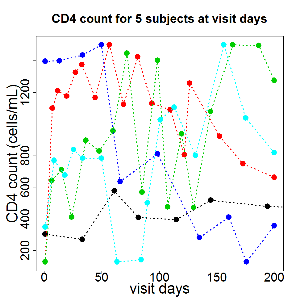
Figure 1: CD4 count and log viral load for $5$ random patients measured at irregularly spaced time points, which are colored by patients.

6.2 Objective

We aim to estimate the averaged causal effect of the time to HAART initiation on the mean CD4 count at year 2 after HIV infection directly on the basis of the original data without discretization. We assume a continuous-time SNMM $\gamma(\overline{V}_{u};\psi^{*})=(\psi_{1}^{*}+\psi_{2}^{*}t)(\tau-t)I(t\leq\tau)$. As discussed before, $\psi_{2}^{*}$ quantifies the impact of time to treatment initiation. The rationale for this modeling choice is because the duration of treatment may well be predictive of its effect.

6.3 Estimator and nuisance models

We consider the proposed estimators $\widehat{\psi}_{\mathrm{cont},1}$ and $\widehat{\psi}_{\mathrm{cont},2}$ specified in Section 5. The estimation procedure requires specifying and fitting nuisance models, which we now consider.

Model for the treatment process. The model for the treatment process $(M_{T})$ is a time-dependent proportional hazards model adjusting for gender, age (age at infection), race (white non-Hispanic race), injdrug (injection drug ever/never), CD4${}_{u}^{1/2}$ (square root of current CD4 count ), lvl_u (log viral load), days from last visit_u (number of days since the last visit), first visit_u (whether the visit is the first visit), second visit_u (whether the visit is the second visit). Table 4 (the left portion) reports the point and standard error estimates of coefficients in the treatment process model. Male and injection drug user are negatively associated with the hazard of treatment initiation, which are significant at the $0.05$ level. Moreover, higher CD4 count and viral load, more days from the last visit, and whether the visit is the first visit are associated with a decreased hazard of treatment initiation.

Model for the censoring process. The model for the censoring process $(K_{C})$ is a time-dependent proportional hazards model adjusting for gender, age, white non-Hispanic race, injdrug, CD4${}_{u}^{1/2}$, lvl_u, and Treated_u (whether a patient had initiated HAART). Table 4 (the right portion) reports the point and standard error estimates of coefficients in the censoring model. Age is negatively associated with the hazard of censoring, while being an injection drug user is positively associated with the hazard of censoring, both are highly significant. Moreover, higher CD4 count, more days from the last visit, and whether the visit is the first visit are highly associated with a decreased hazard of censoring.

Table 4: Fitted time-dependent proportional hazards models for time to treatment initiation and time to censoring

	time to treatment initiation				time to censoring
	Est	SE	p-val		Est	SE	p-val
male	-0.35	0.161	0.03	*	0.21	0.159	0.19
age	0.01	0.003	0.08	.	-0.02	0.004	0.00	***
white non-hispanic	0.12	0.066	0.07	.	0.02	0.077	0.77
injdrug	-0.50	0.180	0.01	**	0.74	0.156	0.00	***
CD4${}_{u}^{1/2}$	-0.06	0.007	0.00	***	-0.03	0.007	0.00	***
lvlu	-0.14	0.013	0.00	***	0.04	0.016	0.02	*
days from last visitu	-0.03	0.002	0.00	***	-0.01	0.001	0.00	***
first visitu	-3.06	0.111	0.00	***	-1.24	0.231	0.00	***
second visitu	-0.04	0.081	0.61		0.68	0.178	0.00	***
Treatedu	–	–	–		-0.15	0.102	0.15

Signif. codes: 0 ’***’ 0.001 ’**’ 0.01 ’*’ 0.05 ’.’

Model for the potential outcome mean function. The outcome model $E\{H(\widehat{\psi}_{p})\mid\overline{V}_{u},T\geq u;\beta\}$ is a linear regression model where the covariates include age, male, race, injdrug, CD4_u, lvl_u, CD4${}_{u}^{3/4}(\tau-u)$, CD4${}_{u}^{3/4}\times(\tau-u)\times$age, CD4${}_{u}^{3/4}\times(\tau-u)\times$male, CD4${}_{u}^{3/4}\times(\tau-u)\times$race, CD4${}_{u}^{3/4}\times(\tau-u)\times$injdrug, CD4${}_{u}^{3/4}\times(\tau-u)\times$lvl_u, CD4slope_u measured, CD4slope${}_{u}\times(\tau-u)^{1/2}$ $I(u\leq 6)(6-u)$, and $I(u\leq 6)(36-u^{2})$. This model specification is motivation based on the substantive literature including Taylor et al. (1994), Taylor and Law (1998), Rodríguez et al. (2006), May et al. (2009).

Other nuisance models. $E(\tau-T\mid\overline{L}_{u},T\geq u)$ and $E\{T(\tau-T)\mid\overline{L}_{u},T\geq u)\}$ are linear regression models where the covariates include $u$, $(\tau-u)$, male$\times(\tau-u)$, age$\times(\tau-u)$, race$\times(\tau-u)$, injdrug$\times(\tau-u)$, CD4${}_{u}^{1/2}$$\times(\tau-u)$, lvl_u$\times(\tau-u)$, days from last visit${}_{u}\times(\tau-u)$, first visit${}_{u}\times(\tau-u)$, second visit${}_{u}\times(\tau-u)$.

The confounding variables and nuisance models are chosen on the basis of the substantive knowledge and the established literature, and therefore the NUC assumption is plausible in this application. We use bootstrap for variance estimation with the bootstrap size $100$ and compute the $95\%$ Wald confidence interval.

6.4 Results

Table 5 shows the results for the effect of time to HAART initiation on the CD4 count at year 2. We note only slight differences in the point estimates between our estimators. Based on our results, on average, initiation of HAART at the time of infection ($t=0$) can increase CD4 counts at year 2 by $14.1\text{cells/mm${}^{3}$ per month}\times 24\text{ months}\approx 338$ cells/mm³; while initiation of HAART $3$ months after the time of infection can increase CD4 counts at year 2 by $(14.1-1.00\times 3)\times(24-3)\approx 233$ cells/mm³.

Table 5: Results of the effect of time to HAART initiation on the CD4 count at year 2

Method	Est	SE	lower .95	upper .95	p-val
	$\psi_{1}^{*}$ cells/mm3 per month
Proposed 1: $\widehat{\psi}_{\mathrm{cont},1}$	14.1	1.1	12.0	16.3	0.000
Proposed 2: $\widehat{\psi}_{\mathrm{cont},2}$	14.3	1.1	12.2	16.6	0.000
	$\psi_{2}^{*}$ cells/mm3 per month2
Proposed 1: $\widehat{\psi}_{\mathrm{cont},1}$	-1.00	0.23	-1.42	-0.50	0.000
Proposed 2: $\widehat{\psi}_{\mathrm{cont},2}$	-1.01	0.23	-1.43	-0.52	0.000

7 Discussion

In this article, we have developed a new semiparametric estimation framework for continuous-time SNMMs to evaluate treatment effects with irregularly spaced longitudinal observations. Our approach does not require specifying the joint distribution of the covariate, treatment, outcome and censoring processes. Moreover, our method achieves a multiple robustness property requiring the correct specification of either the model for the potential outcome mean function or the model for the treatment process, regardless whether the censoring process model is correctly specified. This robustness property will be useful when there is little prior or substantive knowledge about the data processes. Below, we discuss several directions for future work.

7.1 Other types of outcome

To accommodate different types of outcome, we consider a general specification of the continuous-time SNMM as

$$\gamma_{t}(\overline{L}_{t})=g\left[\mathbb{E}\left\{Y^{(t)}\mid\overline{L}_{t},T\geq t\right\}\right]-g\left[\mathbb{E}\left\{Y^{(\infty)}\mid\overline{L}_{t},T\geq t\right\}\right]=\gamma_{t}(\overline{L}_{t};\psi^{*}),$$ (23)

where $g(\cdot)$ is a pre-specified link function. For the continuous outcome, $g(\cdot)$ can be an identity link, i.e. $g(x)=x$, as we adopt in this article. For the binary outcome, $g(\cdot)$ can be a logit link, i.e. $g(x)=\text{logit}(x)\coloneqq\log\{x/(1-x)\}$. Then, (23) specifies the treatment effect on the odds ratio scale, i.e. $\text{odds}\left\{Y^{(t)}\mid\overline{L}_{t},T\geq t\right\}/\text{odds}\left\{Y^{(\infty)}\mid\overline{L}_{t},T\geq t\right\}$, where $\text{odds}(Y\mid X)=P(Y=1\mid X)/P(Y=0\mid X)$. In this case, $H(\psi^{*})$ can be constructed as $H(\psi^{*})=\text{expit}\left[\text{logit}\{\mathbb{E}(Y\mid\overline{L}_{t},T\geq t)\}-\gamma_{t}(\overline{L}_{t};\psi^{*})\right]$. We can develop the corresponding semiparametric efficiency theory for $\psi^{*}$ similarly. For a time to event outcome, we can consider the structural nested failure time models (Robins and Tsiatis, 1991, Robins, 1992, Yang et al., 2019).

7.2 Effect modification and model selection

Effect modification occurs when the magnitude of the treatment effect varies as a function of observed covariates. To allow for time-varying treatment effect modifiers, assume $\gamma_{t}(\overline{V}_{t};\psi^{*})=\{\psi_{1}^{*}+\psi_{2}^{*}t+\psi_{3}^{*\mathrm{\scriptscriptstyle T}}W(t,\overline{V}_{t})\}(\tau-t)I(t\leq\tau)$, when $W(t,\overline{V}_{t})$ is a pre-specified and possibly high-dimensional function of $t$ and $\overline{V}_{t}$. It is important to identify the true treatment effect modifiers, which can facilitate development of optimal treatment strategies in personalized medicine (Murphy, 2003). We will develop a variable selection procedure for identifying effect modifiers. The insight is that we have a larger number of estimating functions than the number of parameters. The problem for effect modifiers selection falls into the recent work of Chang et al. (2018) on high-dimensional statistical inferences with over-identification.

7.3 Sensitivity analysis to the NUC assumption

The key assumption to identify the causal parameters in the continuous-time SNMM is the NUC assumption. However, this assumption is not verifiable based on the observed data. In future studies, it is desirable that the follow-up visits and treatment assignment be determined by study protocol. By formalizing the visit process and treatment assignment, one knows by design which covariates contribute to the treatment process to ensure the NUC assumption holds with all the relevant covariates. In the absence of study protocol, we then recommend conducting sensitivity analysis to assess the impact of possible uncontrolled confounding. For the discrete-time SNMMs, Yang and Lok (2018) assumed a bias function $b(\overline{L}_{m})=\mathbb{E}\{Y^{(\infty)}\mid\overline{A}_{m-1}=\overline{0},A_{m}=1,\overline{L}_{m}\}-\mathbb{E}\{Y^{(\infty)}\mid\overline{A}_{m-1}=\overline{0},A_{m}=0,\overline{L}_{m}\}$ that quantifies the impact of unmeasured confounding and developed a modified g-estimator. For the continuous-time SNMMs, it would also be important to develop a sensitivity analysis methodology, along the lines of Robins et al. (1999) or Yang and Lok (2018), to evaluate the sensitivity of causal inference to departures from the NUC assumption.

Supplementary Material

Supplementary material online includes proofs, technical and simulation details.

Supplementary material for “Structural nested mean models with irregularly spaced observations”

Appendix S1 Proofs

S1.1 Proof of (9)

First, we express

$$\lambda_{T}\{t\mid\overline{V}_{t},Y^{(\infty)}\}=\lim_{h\rightarrow 0}h^{-1}P\{t\leq T<t+h\mid\overline{V}_{t},Y^{(\infty)},T\geq t\}$$

$$= \lim_{h\rightarrow 0}h^{-1}\frac{f\{Y^{(\infty)}\mid\overline{V}_{t},t\leq T<t+h\}P\{t\leq T<t+h\mid\overline{V}_{t},T\geq t\}}{f\{Y^{(\infty)}\mid\overline{V}_{t},T\geq t\}}$$

$$= \lim_{h\rightarrow 0}h^{-1}\frac{f\{H(\psi^{*})\mid\overline{V}_{t},t\leq T<t+h\}P\{t\leq T<t+h\mid\overline{V}_{t},T\geq t\}}{f\{H(\psi^{*})\mid\overline{V}_{t},T\geq t\}}$$

$$= \lim_{h\rightarrow 0}h^{-1}P\{t\leq T<t+h\mid\overline{V}_{t},H(\psi^{*}),T\geq t\}$$

$$= \lambda_{T}\{t\mid\overline{V}_{t},H(\psi^{*})\},$$

where the second equality follows by the Bayes rule, and the third equality follows by Model (7) which implies that the distribution of $\{\overline{V}_{t},Y^{(\infty)}\}$ is the same as the distribution of $\{\overline{V}_{t},H(\psi^{*})\}$.

Second, by Assumption 6, $\lambda_{T}\{t\mid\overline{V}_{t},Y^{(\infty)}\}=\lambda_{T}(t\mid\overline{V}_{t})$. Therefore, $\lambda_{T}\{t\mid\overline{V}_{t},H(\psi^{*})\}=\lambda_{T}\{t\mid\overline{V}_{t},Y^{(\infty)}\}=\lambda_{T}(t\mid\overline{V}_{t})$.

S1.2 Proof of Theorem 1

First, we characterize the semiparametric likelihood function of $\psi^{*}$ based on a single variable $O=(\overline{V}_{\tau},Y)$. The semiparametric likelihood is

$$f_{O}\left(\overline{V}_{\tau},Y\right)=\left\{\frac{\mathrm{d}H(\psi^{*})}{\mathrm{d}Y}\right\}f_{\{\overline{V}_{\tau},H(\psi^{*})\}}\{\overline{V}_{\tau},H(\psi^{*})\}=f_{\{\overline{V}_{\tau},H(\psi^{*})\}}\{\overline{V}_{\tau},H(\psi^{*})\},$$ (S1)

where the first equality follows by the transformation of $O$ to $\{\overline{V}_{\tau},H(\psi^{*})\}$, and the second equality follows because $\mathrm{d}H(\psi^{*})/\mathrm{d}Y=1$. To express (S1) further, we let the observed times to treatment initiation among the $n$ subjects be $v_{0}=0<v_{1}<\cdots<v_{M}$. By Assumption 6 and (9), we express

$$f_{O}\left(\overline{V}_{\tau},Y;\psi^{*},\theta\right) = f\left\{H(\psi^{*});\theta_{1}\right\}\prod_{k=1}^{M}f\left\{L_{v_{k}}\mid\overline{A}_{v_{k-1}}=\overline{0},\overline{L}_{v_{k-1}},H(\psi^{*});\theta_{2}\right\}$$ (S2)

$$\times\prod_{v=v_{1}}^{v_{M}}f\left\{A_{v_{k}}\mid\overline{A}_{v_{k-1}}=\overline{0},\overline{L}_{v_{k}},H(\psi^{*});\theta_{3}\right\},$$

$$= f\left\{H(\psi^{*});\theta_{1}\right\}\prod_{k=1}^{M}f\left\{L_{v_{k}}\mid\overline{A}_{v_{k-1}}=\overline{0},\overline{L}_{v_{k-1}},H(\psi^{*});\theta_{2}\right\}$$

$$\times\prod_{v=v_{1}}^{v_{M}}f\left\{A_{v_{k}}\mid\overline{A}_{v_{k-1}}=\overline{0},\overline{L}_{v_{k}};\theta_{3}\right\}$$

$$= f\left\{H(\psi^{*});\theta_{1}\right\}\prod_{k=1}^{M}f\left\{L_{v_{k}}\mid\overline{A}_{v_{k-1}}=\overline{0},\overline{L}_{v_{k-1}},H(\psi^{*});\theta_{2}\right\}$$

$$\times f(T,\Gamma\mid\overline{V}_{T};\theta_{3}),$$

where $\theta=(\theta_{1},\theta_{2},\theta_{3})$ is a vector of the infinite-dimensional nuisance parameters given the nonparametric models, and the third equality follows because $\prod_{k=1}^{M}f\left(A_{v_{k}}\mid\overline{A}_{v_{k-1}}=\overline{0},\overline{L}_{v_{k}};\theta_{3}\right)$ can be equivalently expressed as the likelihood based on the data $(T,\Gamma)$ given $\overline{V}_{T}$.

Second, we characterize $\Lambda_{k}$, the nuisance tangent space for $\theta_{k},$ for $k=1,2,3$. Assuming $f\left\{H(\psi^{*});\theta_{1}\right\}$ and $\prod_{k=1}^{M}f\left\{L_{v_{k}}\mid\overline{A}_{v_{k-1}}=\overline{0},\overline{L}_{v_{k-1}},H(\psi^{*});\theta_{2}\right\}$ are nonparametric, it follows from Section 4.4 of Tsiatis (2006) that the tangent space regarding $\theta_{1}$ is

$$\Lambda_{1}=\left\{s\left\{H(\psi^{*})\right\}\in\mathbb{\mathbb{R}}^{p}:\mathbb{E}\left[s\left\{H(\psi^{*})\right\}\right]=0\right\},$$

and the tangent space of $\theta_{2}$ is

$$\Lambda_{2}=\sum_{k=1}^{M}\left\{S\left\{\overline{V}_{v_{k}-1},L_{v_{k}},H(\psi^{*})\right\}\in\mathbb{R}^{p}:\right.\\ \left.\mathbb{E}\left[S\left\{\overline{V}_{v_{k}-1},L_{v_{k}},H(\psi^{*})\right\}\mid\overline{A}_{v_{k-1}}=\overline{0},\overline{L}_{v_{k-1}},H(\psi^{*})\right]=0\right\}.$$

By writing

$$f_{(T,\Gamma\mid\overline{V}_{T})}(T,\Gamma\mid\overline{V}_{T})=\lambda_{T}(T\mid\overline{V}_{T})^{\Gamma}\exp\left\{-\int_{0}^{T}\lambda_{T}(u\mid\overline{V}_{u})\mathrm{d}u\right\}\\ \times\left\{f_{T\mid\overline{V}_{T}}(T\mid\overline{V}_{T})\right\}^{1-\Gamma}\left\{\int_{T}^{\infty}f_{T\mid\overline{V}_{T}}(u\mid\overline{V}_{u})\mathrm{d}u\right\}^{\Gamma},$$

it follows from Tsiatis (2006) that the tangent space of $\theta_{3}$ is

$$\Lambda_{3}=\left\{\int h_{u}(\overline{V}_{u})\mathrm{d}M_{T}(u):\text{for all }h_{u}(\overline{V}_{u})\in\mathbb{\mathbb{R}}^{p}\right\}.$$

Then, the nuisance tangent space becomes $\Lambda=\Lambda_{1}\oplus\Lambda_{2}\oplus\Lambda_{3}$, where $\oplus$ denotes a direct sum. This is because $\theta_{1},$ $\theta_{2},$ and $\theta_{3}$ separate out in the likelihood function and therefore $\Lambda_{1}$, $\Lambda_{2}$ and $\Lambda_{3}$ are mutually orthogonal.

Third, we characterize $\Lambda^{\bot}$ using the following technical trick. Define

$$\Lambda_{3}^{*}=\left\{\int h_{u}\{\overline{V}_{u},H(\psi^{*})\}\mathrm{d}M_{T}(u):\ h_{u}\{\overline{V}_{u},H(\psi^{*})\}\in\mathbb{R}^{p}\right\}.$$

Because the tangent space $\Lambda_{1}\oplus\Lambda_{2}\oplus\Lambda_{3}^{*}$ is that for a nonparametric model; i.e., a model that allows for all densities of $O$, and because the tangent space for a nonparametric model is the entire Hilbert space, we obtain that $\mathcal{H}=\Lambda_{1}\oplus\Lambda_{2}\oplus\Lambda_{3}^{*}.$ Because $\Lambda^{\bot}$ must be orthogonal to $\Lambda_{1}\oplus\Lambda_{2}$, $\Lambda^{\bot}$ consists of all elements of $\Lambda_{3}^{*}$ that are orthogonal to $\Lambda_{3}$. It then suffices to find the projection of all elements of $\Lambda_{3}^{*}$, $\int h_{u}\{\overline{V}_{u},H(\psi^{*})\}\mathrm{d}M_{T}(u)$, onto $\Lambda_{3}^{\bot}$. To find the projection, we derive $h_{u}^{*}(\overline{V}_{u})$ such that

$$\left[\int h_{u}\{\overline{V}_{u},H(\psi^{*})\}\mathrm{d}M_{T}(u)-\int h_{u}^{*}(\overline{V}_{u})\mathrm{d}M_{T}(u)\right]\in\Lambda_{3}^{\bot}.$$

Therefore, we have

$$\mathbb{E}\left(\int\left[h_{u}\{\overline{V}_{u},H(\psi^{*})\}-h_{u}^{*}(\overline{V}_{u})\right]\mathrm{d}M_{T}(u)\times\int h_{u}(\overline{V}_{u})\mathrm{d}M_{T}(u)\right)=0,$$ (S3)

for any $h_{u}(\overline{V}_{u})$. It is important to note that by Assumption 6, $M_{T}(t)$ is a martingale with respect to the filtration $\sigma\{\overline{V}_{t},H(\psi^{*})\}$. If $P_{1}(u)$ and $P_{2}(u)$ are locally bounded $\sigma\{\overline{V}_{t},H(\psi^{*})\}$-predictable processes, then we have the following useful result:

$$\mathbb{E}\left\{\int_{0}^{t}P_{1}(u)\mathrm{d}M_{T}(u)\int_{0}^{t}P_{2}(u)\mathrm{d}M_{T}(u)\right\}=\int_{0}^{t}P_{1}(u)P_{2}(u)\lambda_{T}(u\mid\overline{V}_{u})Y_{T}(u)\mathrm{d}u.$$ (S4)

By (S4), (S3) becomes

$$\mathbb{E}\left(\int\left[h_{u}\{\overline{V}_{u},H(\psi^{*})\}-h_{u}^{*}(\overline{V}_{u})\right]h_{u}(\overline{V}_{u})\lambda_{T}(u\mid\overline{V}_{u})Y_{T}(u)\mathrm{d}u\right)\\ =\mathbb{E}\left(\int\mathbb{E}\left(\left[h_{u}\{\overline{V}_{u},H(\psi^{*})\}-h_{u}^{*}(\overline{V}_{u})\right]Y_{T}(u)\mid\overline{V}_{u}\right)h_{u}(\overline{V}_{u})\lambda_{T}(u\mid\overline{V}_{u})\mathrm{d}u\right)=0,$$

for any $h_{u}(\overline{V}_{u})$. Because $h_{u}(\overline{V}_{u})$ is arbitrary, we obtain

$$\mathbb{E}\left(\left[h_{u}\{\overline{V}_{u},H(\psi^{*})\}-h_{u}^{*}(\overline{V}_{u})\right]Y_{T}(u)\mid\overline{V}_{u}\right)=0.$$ (S5)

Solving (S5) for $h_{u}^{*}(\overline{V}_{u})$, we obtain

$$h_{u}^{*}(\overline{V}_{u})=\mathbb{E}\left[h_{u}\{\overline{V}_{u},H(\psi^{*})\}\mid\overline{V}_{u},T\geq u\right].$$

This completes the proof.

S1.3 Proof of Theorem 2

For any $B=B(F)$, let

$$G=G(F)=\int_{0}^{\tau}\left[\mathbb{E}\left\{B\dot{H}_{u}(\psi^{*})\mid\overline{V}_{u},T=u\right\}-\mathbb{E}\left\{B\dot{H}_{u}(\psi^{*})\mid\overline{V}_{u},T\geq u\right\}\right]\\ \times\left[\mathrm{var}\left\{H(\psi^{*})\mid\overline{V}_{u},T\geq u\right\}\right]^{-1}\left[H(\psi^{*})-\mathbb{E}\left\{H(\psi^{*})\mid\overline{V}_{u},T\geq u\right\}\right]\mathrm{d}M_{T}(u).$$

To show $\prod\left(B\mid\Lambda^{\bot}\right)=G$, it is easy to see that $G\in\Lambda^{\bot},$ so the remaining is to show that $B-G\in\Lambda$. Toward this end, we show that for any $\tilde{G}=\tilde{G}(F)=\int_{0}^{\tau}\tilde{c}(\overline{V}_{u})[H(\psi^{*})-\mathbb{E}\{H(\psi^{*})\mid\overline{V}_{u},T\geq u\}]Y_{T}(u)\mathrm{d}M_{T}(u)\in\Lambda^{\bot}$, $(B-G)\mathbin{\mathchoice{\hbox to0.0pt{\hbox{$\displaystyle\perp$}\hss}\kern 3.46875pt{}\kern 3.46875pt\hbox{$\displaystyle\perp$}}{\hbox to0.0pt{\hbox{$\textstyle\perp$}\hss}\kern 3.46875pt{}\kern 3.46875pt\hbox{$\textstyle\perp$}}{\hbox to0.0pt{\hbox{$\scriptstyle\perp$}\hss}\kern 2.36812pt{}\kern 2.36812pt\hbox{$\scriptstyle\perp$}}{\hbox to0.0pt{\hbox{$\scriptscriptstyle\perp$}\hss}\kern 1.63437pt{}\kern 1.63437pt\hbox{$\scriptscriptstyle\perp$}}}\tilde{G}$ or $\mathbb{E}\{(B-G)\tilde{G}\}=0$. We now verify $\mathbb{E}(B\tilde{G})=\mathbb{E}(G\tilde{G})$ by the following calculation.

First, by (S4), we calculate

$$\mathbb{E}\left(G\tilde{G}\right) = \mathbb{E}\int_{0}^{\tau}\tilde{c}(\overline{V}_{u})[\mathbb{E}\{B\dot{H}_{u}(\psi^{*})\mid\overline{V}_{u},T=u\}-\mathbb{E}\{B\dot{H}_{u}(\psi^{*})\mid\overline{V}_{u},T\geq u\}]$$ (S6)

$$\times[\mathrm{var}\{H(\psi^{*})\mid\overline{V}_{u},T\geq u\}]^{-1}[H(\psi^{*})-\mathbb{E}\{H(\psi^{*})\mid\overline{V}_{u},T\geq u\}]{}^{2}$$

$$\times\lambda_{T}(u\mid\overline{V}_{u})Y_{T}(u)\mathrm{d}u$$

$$= \mathbb{E}\int_{0}^{\tau}\tilde{c}(\overline{V}_{u})[\mathbb{E}\{B\dot{H}_{u}(\psi^{*})\mid\overline{V}_{u},T=u\}-\mathbb{E}\{B\dot{H}_{u}(\psi^{*})\mid\overline{V}_{u},T\geq u\}]$$

$$\times\lambda_{T}(u\mid\overline{V}_{u})Y_{T}(u)\mathrm{d}u.$$

Second, we calculate

$$\mathbb{E}\left(B\tilde{G}\right) = \mathbb{E}\int_{0}^{\tau}\tilde{c}(\overline{V}_{u})B[H(\psi^{*})-\mathbb{E}\{H(\psi^{*})\mid\overline{L}_{u},T\geq u\}]\mathrm{d}M_{T}(u)$$ (S7)

$$= \mathbb{E}\int_{0}^{\tau}\tilde{c}(\overline{V}_{u})B\dot{H}_{u}(\psi^{*})\mathrm{d}N_{T}(u)$$

$$-\mathbb{E}\int_{0}^{\tau}\tilde{c}(\overline{V}_{u})B\dot{H}_{u}(\psi^{*})\lambda_{T}(u\mid\overline{V}_{u})Y_{T}(u)\mathrm{d}u$$

$$= \mathbb{E}\int_{0}^{\tau}\tilde{c}(\overline{V}_{u})[\mathbb{E}\{B\dot{H}_{u}(\psi^{*})\mid\overline{V}_{u},T=u\}-\mathbb{E}\{B\dot{H}_{u}(\psi^{*})\mid\overline{V}_{u},T\geq u\}]$$

$$\times\lambda_{T}(u\mid\overline{V}_{u})Y_{T}(u)\mathrm{d}u,$$

where the last equality follows because

$$\mathbb{E}\int_{0}^{\tau}\tilde{c}(\overline{V}_{u})B\dot{H}_{u}(\psi^{*})\mathrm{d}N_{T}(u)=\mathbb{E}\int_{0}^{\tau}\tilde{c}(\overline{V}_{u})\mathbb{E}\{B\dot{H}_{u}(\psi^{*})\mid\overline{V}_{u},T\}\mathrm{d}N_{T}(u)\\ =\mathbb{E}\int_{0}^{\tau}\tilde{c}(\overline{V}_{u})\mathbb{E}\{B\dot{H}_{u}(\psi^{*})\mid\overline{V}_{u},T=u\}\lambda_{T}(u\mid\overline{V}_{u})Y_{T}(u)\mathrm{d}u,$$

and

$$\mathbb{E}\left\{\int_{0}^{\tau}\tilde{c}(\overline{V}_{u})B\dot{H}_{u}(\psi^{*})\lambda_{T}(u\mid\overline{V}_{u})Y_{T}(u)\mathrm{d}u\right\}$$

$$= \mathbb{E}\left[\int_{0}^{\tau}\tilde{c}(\overline{V}_{u})\mathbb{E}\{B\dot{H}_{u}(\psi^{*})\mid\overline{V}_{u},Y_{T}(u)\}\lambda_{T}(u\mid\overline{V}_{u})Y_{T}(u)\mathrm{d}u\right]$$

$$= \mathbb{E}\left[\int_{0}^{\tau}\tilde{c}(\overline{V}_{u})\mathbb{E}\{B\dot{H}_{u}(\psi^{*})\mid\overline{V}_{u},T\geq u\}\lambda_{T}(u\mid\overline{V}_{u})Y_{T}(u)\mathrm{d}u\right].$$

Therefore, by (S6) and (S7), $\mathbb{E}(B\tilde{G})=\mathbb{E}(G\tilde{G})$ for any $\tilde{G}\in\Lambda^{\bot}$, proving (11).

S1.4 Proof of Theorem 3

The semiparametric efficient score is $S_{\mathrm{eff}}^{*}(\psi^{*})=\prod\left(S_{\psi}\mid\Lambda^{\bot}\right)$. By Theorem 2, we have

$$S_{\mathrm{eff}}^{*}(\psi^{*}) = \int_{0}^{\tau}[\mathbb{E}\{S_{\psi}\dot{H}_{u}(\psi^{*})\mid\overline{V}_{u},T=u\}-\mathbb{E}\{S_{\psi}\dot{H}_{u}(\psi^{*})\mid\overline{V}_{u},T\geq u\}]$$

$$\times[\mathrm{var}\{H(\psi^{*})\mid\overline{V}_{u},T\geq u\}]{}^{-1}[H(\psi^{*})-\mathbb{E}\{H(\psi^{*})\mid\overline{V}_{u},T\geq u\}]\mathrm{d}M_{T}(u)$$

$$= -\int_{0}^{\tau}[\mathbb{E}\{\partial\dot{H}_{u}(\psi^{*})/\partial\psi\mid\overline{V}_{u},T=u\}-\mathbb{E}\{\partial\dot{H}_{u}(\psi^{*})/\partial\psi\mid\overline{V}_{u},T\geq u\}]$$

$$\times[\mathrm{var}\{H(\psi^{*})\mid\overline{V}_{u},T\geq u\}]{}^{-1}[H(\psi^{*})-\mathbb{E}\{H(\psi^{*})\mid\overline{V}_{u},T\geq u\}]\mathrm{d}M_{T}(u)$$

$$= -\int_{0}^{\tau}\mathbb{E}\{\partial\dot{H}_{u}(\psi^{*})/\partial\psi\mid\overline{V}_{u},T=u\}[\mathrm{var}\{H(\psi^{*})\mid\overline{V}_{u},T\geq u\}]^{-1}$$

$$\times H(\psi^{*})-\mathbb{E}\{H(\psi^{*})\mid\overline{V}_{u},T\geq u\}]\mathrm{d}M_{T}(u),$$

where the last equality follows by using the generalized information equality: because $\dot{H}_{u}(\psi^{*})=H(\psi^{*})-\mathbb{E}\{H(\psi^{*})\mid\overline{V}_{u},T\geq u\}$, we have $\mathbb{E}\{\dot{H}_{u}(\psi^{*})\mid\overline{V}_{u},T\geq u\}=0$. Take the derivative of $\psi$ at both sides, we have $\mathbb{E}\{S_{\psi}\dot{H}_{u}(\psi^{*})\mid\overline{V}_{u},T\geq u\}+\mathbb{E}\{\partial\dot{H}_{u}(\psi^{*})/\partial\psi\mid\overline{V}_{u},T\geq u\}=0$, or equivalently $\mathbb{E}\{S_{\psi}\dot{H}_{u}(\psi^{*})\mid\overline{V}_{u},T\geq u\}=-\mathbb{E}\{\partial\dot{H}_{u}(\psi^{*})/\partial\psi\mid\overline{V}_{u},T\geq u\}$. Similarly, noticing $\mathbb{E}\{H(\psi^{*})\mid\overline{V}_{u},T\geq u\}=\mathbb{E}\{H(\psi^{*})\mid\overline{V}_{u},T=u\}$, we have $\mathbb{E}\{\dot{H}_{u}(\psi^{*})\mid\overline{V}_{u},T=u\}=0$. Take the derivative of $\psi$ at both sides, we have $\mathbb{E}\{S_{\psi}\dot{H}_{u}(\psi^{*})\mid\overline{V}_{u},T=u\}+\mathbb{E}\{\partial\dot{H}_{u}(\psi^{*})/\partial\psi\mid\overline{V}_{u},T=u\}=0$, or equivalently $\mathbb{E}\{S_{\psi}\dot{H}_{u}(\psi^{*})\mid\overline{V}_{u},T=u\}=-\mathbb{E}\{\partial\dot{H}_{u}(\psi^{*})/\partial\psi\mid\overline{V}_{u},T=u\}$. Ignoring the negative sign, the result in Theorem 3 follow.

S1.5 Proof of Theorem 4

We show that $\mathbb{E}\{G(\psi^{*};F,c)\}=0$ in two cases.

First, if $\lambda_{T}(t\mid\overline{V}_{t})$ is correctly specified, under Assumption 6, $M_{T}(t)$ is a martingale with respect to the filtration $\sigma\{\overline{V}_{t},H(\psi^{*})\}$. Because $c(\overline{V}_{u})[H(\psi^{*})-\mathbb{E}\{H(\psi^{*})\mid\overline{V}_{u},T\geq u\}]$ is a $\sigma\{\overline{V}_{t},H(\psi^{*})\}$-predictable process, $\int_{0}^{t}c(\overline{V}_{u})[H(\psi^{*})-\mathbb{E}\{H(\psi^{*})\mid\overline{V}_{u},T\geq u\}]\mathrm{d}M_{T}(u)$ is a martingale for $t\geq 0$. Therefore, $\mathbb{E}\{G(\psi^{*};F,c)\}=0$.

Second, if $\mathbb{E}\left\{H(\psi^{*})\mid\overline{V}_{u},T\geq u\right\}$ is correctly specified but $\lambda_{T}(t\mid\overline{V}_{t})$ is not necessarily correctly specified, let $\lambda_{T}^{*}(t\mid\overline{V}_{t})$ be the probability limit of the possibly misspecified model. We obtain

$$\mathbb{E}\int c(\overline{V}_{u})\left[H(\psi^{*})-\mathbb{E}\left\{H(\psi^{*})\mid\overline{V}_{u},T\geq u;\beta^{*}\right\}\right]\left\{\mathrm{d}N_{T}(u)-\lambda_{T}^{*}(u\mid\overline{V}_{u})Y_{T}(u)\mathrm{d}u\right\}$$

$$= \mathbb{E}\int c(\overline{V}_{u})\left[H(\psi^{*})-\mathbb{E}\left\{H(\psi^{*})\mid\overline{V}_{u},T\geq u;\beta^{*}\right\}\right]\left\{\mathrm{d}N_{T}(u)-\lambda_{T}(u\mid\overline{V}_{u})Y_{T}(u)\mathrm{d}u\right\}$$

$$+\mathbb{E}\int c(\overline{V}_{u})\left[H(\psi^{*})-\mathbb{E}\left\{H(\psi^{*})\mid\overline{V}_{u},T\geq u;\beta^{*}\right\}\right]\left\{\lambda_{T}(u\mid\overline{V}_{u})-\lambda_{T}^{*}(u\mid\overline{V}_{u})\right\}Y_{T}(u)\mathrm{d}u$$

$$= 0+\mathbb{E}\int c(\overline{V}_{u})E\left(\left[H(\psi^{*})-\mathbb{E}\left\{H(\psi^{*})\mid\overline{V}_{u},T\geq u;\beta^{*}\right\}\right]\mid\overline{V}_{u},T\geq u\right)$$

$$\times\left\{\lambda_{T}(u\mid\overline{V}_{u})-\lambda_{T}^{*}(u\mid\overline{V}_{u})\right\}Y_{T}(u)\mathrm{d}u$$

$$= 0+\mathbb{E}\int c(\overline{V}_{u})\times 0\times\left\{\lambda_{T}(u\mid\overline{V}_{u})-\lambda_{T}^{*}(u\mid\overline{V}_{u})\right\}Y_{T}(u)\mathrm{d}u=0,$$ (S9)

where zero in (S1.5) follows because $\mathrm{d}M_{T}(u)=\mathrm{d}N_{T}(u)-\lambda_{T}(u\mid\overline{V}_{u})\mathrm{d}u$ is a martingale with respect to the filtration $\sigma\{\overline{V}_{t},H(\psi^{*})\}$, and zero in (S9) follows because $\mathbb{E}\left\{H(\psi^{*})\mid\overline{V}_{u},T\geq u\right\}$ is correctly specified and therefore, $\mathbb{E}\left\{H(\psi^{*})\mid\overline{V}_{u},T\geq u;\beta^{*}\right\}=\mathbb{E}\left\{H(\psi^{*})\mid\overline{V}_{u},T\geq u\right\}$.

S1.6 Proof of Theorem 5

We show that $\mathbb{E}\left\{\delta_{C}G(\psi^{*},\beta^{*},M_{T}^{*};F)/K_{C}^{*}(\tau\mid\overline{V}_{\tau})\right\}=0$ in three cases.

First, under Scenarios (a), (b), and (c) listed in Table 1 when $K_{C}^{*}$ is correctly specified for $K_{C}$, either $\mathbb{E}\{H(\psi^{*})\mid\overline{V}_{u},T\geq u;\beta^{*}\}$ is correctly specified or $M_{T}^{*}$ is correctly specified for $M_{T}$, we show that (18) is an unbiased estimating equation. Under these scenarios, we have $K_{C}^{*}(\tau\mid\overline{V}_{\tau})=K_{C}(\tau\mid\overline{V}_{\tau})$. It suffices to show that

$$\mathbb{E}\left\{\frac{\delta_{C}}{K_{C}\left(\tau\mid\overline{V}_{\tau}\right)}G(\psi^{*},\beta^{*},M_{T}^{*};F)\right\} = \mathbb{E}\left[\mathbb{E}\left\{\frac{\delta_{C}}{K_{C}\left(\tau\mid\overline{V}_{\tau}\right)}G(\psi^{*},\beta^{*},M_{T}^{*};F)\mid F\right\}\right]$$

$$= \mathbb{E}\left\{\frac{\mathbb{E}(\delta_{C}\mid F)}{K_{C}\left(\tau\mid\overline{V}_{\tau}\right)}G(\psi^{*},\beta^{*},M_{T}^{*};F)\right\}$$

$$= \mathbb{E}\left[\frac{\mathbb{E}(\delta_{C}\mid\overline{V}_{\tau})}{K_{C}\left(\tau\mid\overline{V}_{\tau}\right)}\mathbb{E}\{G(\psi^{*},\beta^{*},M_{T}^{*};F)\mid\overline{V}_{\tau}\}\right],$$

where the third equality follows by Assumption 7, and the last equality follows by Theorem 4.

Second, under Scenarios (b) and (d) listed in Table 1 when $\mathbb{E}\{H(\psi^{*})\mid\overline{V}_{u},T\geq u;\beta^{*}\}$ is correctly specified, we have $\mathbb{E}\{H(\psi^{*})\mid\overline{V}_{u},T\geq u;\beta^{*}\}=\mathbb{E}\{H(\psi^{*})\mid\overline{V}_{u},T\geq u\}$. Also, under Assumption 6, $\mathbb{E}\left\{H(\psi^{*})\mid\overline{V}_{u},T\geq u\right\}=\mathbb{E}\left\{H(\psi^{*})\mid\overline{V}_{u}\right\}$. Then, we have

$$\mathbb{E}\{G(\psi^{*},\beta^{*},M_{T}^{*};F)\mid\overline{V}_{\tau}\}$$

$$= \mathbb{E}\left\{\int c(\overline{V}_{u})\left[H(\psi^{*})-\mathbb{E}\left\{H(\psi^{*})\mid\overline{V}_{u},T\geq u;\beta^{*}\right\}\right]\mathrm{d}M_{T}^{*}(u)\mid\overline{V}_{\tau}\right\}$$

$$= \int c(\overline{V}_{u})\mathbb{E}\left[H(\psi^{*})-\mathbb{E}\left\{H(\psi^{*})\mid\overline{V}_{u},T\geq u\right\}\mid\overline{V}_{\tau}\right]\mathbb{E}\left\{\mathrm{d}M_{T}^{*}(u)\mid\overline{V}_{\tau}\right\}$$

$$= \int c(\overline{V}_{u})\mathbb{E}\left[\mathbb{E}\left\{H(\psi^{*})\mid\overline{V}_{u}\right\}-\mathbb{E}\left\{H(\psi^{*})\mid\overline{V}_{u},T\geq u\right\}\mid\overline{V}_{\tau}\right]\mathbb{E}\left\{\mathrm{d}M_{T}^{*}(u)\mid\overline{V}_{\tau}\right\}$$

$$= \int c(\overline{V}_{u})\mathbb{E}\left[\mathbb{E}\left\{H(\psi^{*})\mid\overline{V}_{u},T\geq u\right\}-\mathbb{E}\left\{H(\psi^{*})\mid\overline{V}_{u},T\geq u\right\}\mid\overline{V}_{\tau}\right]\mathbb{E}\left\{\mathrm{d}M_{T}^{*}(u)\mid\overline{V}_{\tau}\right\}=0.$$

It follows that

$$\mathbb{E}\left\{\frac{\delta_{C}}{K_{C}^{*}\left(\tau\mid\overline{V}_{\tau}\right)}G(\psi^{*},\beta^{*},M_{T}^{*};F)\right\} = \mathbb{E}\left[\mathbb{E}\left\{\frac{\delta_{C}}{K_{C}^{*}\left(\tau\mid\overline{V}_{\tau}\right)}G(\psi^{*},\beta^{*},M_{T}^{*};F)\mid F\right\}\right]$$

$$= \mathbb{E}\left[\frac{K_{C}\left(\tau\mid\overline{V}_{\tau}\right)}{K_{C}^{*}\left(\tau\mid\overline{V}_{\tau}\right)}\mathbb{E}\{G(\psi^{*},\beta^{*},M_{T}^{*};F)\mid\overline{V}_{\tau}\}\right]$$

$$= \mathbb{E}\left\{\frac{K_{C}\left(\tau\mid\overline{V}_{\tau}\right)}{K_{C}^{*}\left(\tau\mid\overline{V}_{\tau}\right)}\times 0\right\}=0.$$

Third, under Scenario (e) listed in Table 1 when $M_{T}^{*}$ is correctly specified for $M_{T}$, we have

$$\mathbb{E}\left\{\mathrm{d}M_{T}(u)\mid\overline{V}_{u}\right\}=0,\ (u>0).$$ (S10)

Define $\kappa(\overline{V}_{u})=E\left\{K_{C}\left(\tau\mid\overline{V}_{\tau}\right)/K_{C}^{*}\left(\tau\mid\overline{V}_{\tau}\right)\mid\overline{V}_{u}\right\}$ for all $u>0$. We show $\mathbb{E}\left\{\delta_{C}G(\psi^{*},\beta^{*},M_{T};F)/K_{C}^{*}(\tau\mid\overline{V}_{\tau})\right\}=0$ by induction. Let $\Delta>0$ be a small increment. We start with

$$\mathbb{E}\left\{\frac{\delta_{C}}{K_{C}^{*}\left(\tau\mid\overline{V}_{\tau}\right)}G(\psi^{*},\beta^{*},M_{T};F)\right\}$$

$$= \mathbb{E}\left[\kappa(\overline{V}_{\tau})\int_{0}^{\tau}c(\overline{V}_{u})\left[H(\psi^{*})-\mathbb{E}\left\{H(\psi^{*})\mid\overline{V}_{u},T\geq u;\beta^{*}\right\}\right]\mathrm{d}M_{T}(u)\right]$$

$$= \mathbb{E}\left[\kappa(\overline{V}_{\tau})\mathbb{E}\left\{\left(\int_{0}^{\tau-\Delta}+\int_{\tau-\Delta}^{\tau}\right)c(\overline{V}_{u})\left[H(\psi^{*})-\mathbb{E}\left\{H(\psi^{*})\mid\overline{V}_{u},T\geq u;\beta^{*}\right\}\right]\mathrm{d}M_{T}(u)\mid\overline{V}_{\tau}\right\}\right]$$

$$= \mathbb{E}\left[\mathbb{E}\left\{\kappa(\overline{V}_{\tau})\mid\overline{V}_{\tau-\Delta}\right\}\int_{0}^{\tau-\Delta}c(\overline{V}_{u})\left[\mathbb{E}\left\{H(\psi^{*})\mid\overline{V}_{u},T\geq u\right\}-\mathbb{E}\left\{H(\psi^{*})\mid\overline{V}_{u},T\geq u;\beta^{*}\right\}\right]\mathrm{d}M_{T}(u)\right]$$

$$+\mathbb{E}\left\{\kappa(\overline{V}_{\tau})\int_{\tau-\Delta}^{\tau}c(\overline{V}_{u})\left[\mathbb{E}\left\{H(\psi^{*})\mid\overline{V}_{u},T\geq u\right\}-\mathbb{E}\left\{H(\psi^{*})\mid\overline{V}_{u},T\geq u;\beta^{*}\right\}\right]\mathrm{d}M_{T}(u)\right\}$$

$$= \mathbb{E}\left\{\kappa(\overline{V}_{\tau-\Delta})\int_{0}^{\tau-\Delta}c(\overline{V}_{u})\left[\mathbb{E}\left\{H(\psi^{*})\mid\overline{V}_{u},T\geq u\right\}-\mathbb{E}\left\{H(\psi^{*})\mid\overline{V}_{u},T\geq u;\beta^{*}\right\}\right]\mathrm{d}M_{T}(u)\right\}$$

$$+\mathbb{E}\left\{\kappa(\overline{V}_{\tau})c(\overline{V}_{\tau})\left[\mathbb{E}\left\{H(\psi^{*})\mid\overline{V}_{\tau},T\geq\tau\right\}-\mathbb{E}\left\{H(\psi^{*})\mid\overline{V}_{\tau},T\geq\tau;\beta^{*}\right\}\right]\mathbb{E}\left\{\mathrm{d}M_{T}(\tau)\mid\overline{V}_{\tau}\right\}\right\}$$

$$= \mathbb{E}\left\{\left[\kappa(\overline{V}_{\tau-\Delta})\int_{0}^{\tau-\Delta}c(\overline{V}_{u})\left[\mathbb{E}\left\{H(\psi^{*})\mid\overline{V}_{u},T\geq u\right\}-\mathbb{E}\left\{H(\psi^{*})\mid\overline{V}_{u},T\geq u;\beta^{*}\right\}\right]\mathrm{d}M_{T}(u)\right]\right\}+0,$$ (S12)

where $0$ in the last equality follows by (S10). Note that (S12) is (S1.6) replacing $\tau$ by $\tau-\Delta$. We then repeat the same calculation for (S12) until $\tau-\Delta$ reaches zero. The last step is to recognize that (S12) with $\tau-\Delta=0$ is zero. This completes the proof.

S1.7 Proof of Theorem 6

We assume the multiple robustness condition holds; i.e. either the potential outcome mean model or the model for the treatment process is correctly specified, regardless the model for the censoring process is correctly specified.

Taylor expansion of $\mathbb{P}_{n}\left\{\Phi(\widehat{\psi},\widehat{\beta},\widehat{M}_{T},\widehat{K}_{C};F)\right\}=0$ around $\psi^{*}$ leads to

$$0 = \mathbb{P}_{n}\left\{\Phi(\widehat{\psi},\widehat{\beta},\widehat{M}_{T},\widehat{K}_{C};F)\right\}$$

$$= \mathbb{P}_{n}\left\{\Phi(\psi^{*},\widehat{\beta},\widehat{M}_{T},\widehat{K}_{C};F)\right\}+\mathbb{P}_{n}\left\{\frac{\partial\Phi(\widetilde{\psi},\widehat{\beta},\widehat{M}_{T},\widehat{K}_{C};F)}{\partial\psi^{\mathrm{\scriptscriptstyle T}}}\right\}(\widehat{\psi}-\psi^{*}),$$

where $\widetilde{\psi}$ is on the line segment between $\widehat{\psi}$ and $\psi^{*}$.

Under Assumption 9 (i) and (ii),

$$(\mathbb{P}_{n}-\mathbb{P})\left\{\frac{\partial\Phi(\widetilde{\psi},\widehat{\beta},\widehat{M}_{T},\widehat{K}_{C};F)}{\partial\psi^{\mathrm{\scriptscriptstyle T}}}\right\}=(\mathbb{P}_{n}-\mathbb{P})\left\{\frac{\partial\Phi(\psi^{*},\beta^{*},M_{T}^{*},K_{C}^{*};F)}{\partial\psi^{\mathrm{\scriptscriptstyle T}}}\right\}=o_{p}(n^{-1/2}),$$

and therefore,

$$\mathbb{P}_{n}\left\{\frac{\partial\Phi(\widetilde{\psi},\widehat{\beta},\widehat{M}_{T},\widehat{K}_{C};F)}{\partial\psi^{\mathrm{\scriptscriptstyle T}}}\right\} = \mathbb{P}\left\{\frac{\partial\Phi(\widetilde{\psi},\widehat{\beta},\widehat{M}_{T},\widehat{K}_{C};F)}{\partial\psi^{\mathrm{\scriptscriptstyle T}}}\right\}+o_{p}(n^{-1/2})$$

$$= A(\psi^{*},\beta^{*},M_{T}^{*},K_{C}^{*})+o_{p}(n^{-1/2}).$$

We then have

$$n^{1/2}(\widehat{\psi}-\psi^{*})=\left\{A(\psi^{*},\beta^{*},M_{T}^{*},K_{C}^{*})\right\}^{-1}n^{1/2}\mathbb{P}_{n}\left\{\Phi(\psi^{*},\widehat{\beta},\widehat{M}_{T},\widehat{K}_{C};F)\right\}+o_{p}(1).$$ (S13)

Based on the multiple robustness, we have

$$\mathbb{P}\{\Phi(\psi^{*},\beta^{*},M_{T}^{*},K_{C}^{*};F)\}=0.$$ (S14)

To express (S13) further, based on (S14), we have

$$\mathbb{P}_{n}\Phi(\psi^{*},\widehat{\beta},\widehat{M}_{T},\widehat{K}_{C};F)=(\mathbb{P}_{n}-\mathbb{P})\Phi(\psi^{*},\widehat{\beta},\widehat{M}_{T},\widehat{K}_{C};F)\\ +\mathbb{P}\left\{\Phi(\psi^{*},\widehat{\beta},\widehat{M}_{T},\widehat{K}_{C};F)-\Phi(\psi^{*},\beta^{*},M_{T}^{*},K_{C}^{*};F)\right\}+\mathbb{P}\Phi(\psi^{*},\beta^{*},M_{T}^{*},K_{C}^{*};F).$$ (S15)

By Assumption 9 (i) and (ii), the first term in (S5) becomes

$$(\mathbb{P}_{n}-\mathbb{P})\Phi(\psi^{*},\widehat{\beta},\widehat{M}_{T},\widehat{K}_{C};F) = (\mathbb{P}_{n}-\mathbb{P})\Phi(\psi^{*},\beta^{*},M_{T}^{*},K_{C}^{*};F)+o_{p}(n^{-1/2})$$ (S16)

$$= \mathbb{P}_{n}\Phi(\psi^{*},\beta^{*},M_{T}^{*},K_{C}^{*};F)+o_{p}(n^{-1/2}).$$

By Assumption 9 (iv), the second term in (S5) becomes

$$\mathbb{P}\left\{\Phi(\psi^{*},\widehat{\beta},\widehat{M}_{T},\widehat{K}_{C};F)-\Phi(\psi^{*},\beta^{*},M_{T}^{*},K_{C}^{*};F)\right\}$$ (S17)

$$= J(\widehat{\beta},\widehat{M}_{T},\widehat{K}_{C})-J(\beta^{*},M_{T}^{*},K_{C}^{*})+o_{p}(n^{-1/2})$$

$$= J_{1}(\widehat{\beta})-J_{1}(\beta^{*})+J_{2}(\widehat{M}_{T})-J_{2}(M_{T}^{*})+J_{3}(\widehat{K}_{C})-J_{3}(M_{C}^{*})+o_{p}(n^{-1/2})$$

$$= \mathbb{P}_{n}\Phi_{1}(\psi^{*},\beta^{*},M_{T}^{*},K_{C}^{*};F)+\mathbb{P}_{n}\Phi_{2}(\psi^{*},\beta^{*},M_{T}^{*},K_{C}^{*};F)$$

$$+\mathbb{P}_{n}\Phi_{3}(\psi^{*},\beta^{*},M_{T}^{*},K_{C}^{*};F).$$

Combining (S14)–(S17),

$$\mathbb{P}_{n}\Phi(\psi^{*},\widehat{\beta},\widehat{M}_{T},\widehat{K}_{C};F)=\mathbb{P}_{n}\{\widetilde{B}(\psi^{*},\beta^{*},M_{T}^{*},K_{C}^{*};F)\},$$

where

$$\widetilde{B}(\psi^{*},\beta^{*},M_{T}^{*},K_{C}^{*};F) = \Phi(\psi^{*},\beta^{*},M_{T}^{*},K_{C}^{*};F)+\Phi_{1}(\psi^{*},\beta^{*},M_{T}^{*},K_{C}^{*};F)$$

$$+\Phi_{2}(\psi^{*},\beta^{*},M_{T}^{*},K_{C}^{*};F)+\Phi_{3}(\psi^{*},\beta^{*},M_{T}^{*},K_{C}^{*};F).$$

As a result,

$$n^{1/2}(\widehat{\psi}-\psi^{*})=n^{1/2}\mathbb{P}_{n}\widetilde{\Phi}(\psi^{*},\beta^{*},K_{V}^{*},K_{C}^{*};F)+o_{p}(1),$$ (S18)

where

$$\widetilde{\Phi}(\psi^{*},\beta^{*},M_{T}^{*},K_{C}^{*};F)=\left\{A(\psi^{*},\beta^{*},M_{T}^{*},K_{C}^{*})\right\}^{-1}\widetilde{B}(\psi^{*},\beta^{*},M_{T}^{*},K_{C}^{*};F).$$

We now consider the case when all nuisance models are correctly specified, i.e., $\mathbb{E}\{H(\psi^{*})\mid\overline{V}_{u},T\geq u;\beta^{*}\}=\mathbb{E}\{H(\psi^{*})\mid\overline{V}_{u},T\geq u\}$, $M_{T}^{*}=M_{T},$ and $K_{C}^{*}=K_{C}$.

Define the score functions: $S_{\beta}=S_{\beta}\{H(\psi^{*}),\overline{V}_{u},T\geq u\}$. Then, the tangent space for $\beta$ is $\widetilde{\Lambda}_{1}=\{S_{\beta}\in\mathbb{R}^{p}:\mathbb{E}(S_{\beta}\mid\overline{V}_{u},T\geq u)=0\}$. Following Tsiatis (2006), the nuisance tangent space for the proportional hazards model (16) is

$$\widetilde{\Lambda}_{2}=\left\{S_{\alpha}+\int h(u)\mathrm{d}M_{T}(u):\ h(u)\in\mathbb{\mathbb{R}}^{p}\right\},$$

where

$$S_{\alpha}\coloneqq\int\left\{W_{T}(u,\overline{V}_{u})-\frac{\mathbb{E}\left[W_{T}(u,\overline{V}_{u})\exp\left\{\gamma^{\mathrm{\scriptscriptstyle T}}W_{T}(u,\overline{V}_{u})\right\}Y_{T}(u)\right]}{\mathbb{E}\left[\exp\left\{\alpha^{\mathrm{\scriptscriptstyle T}}W_{T}(u,\overline{V}_{u})\right\}Y_{T}(u)\right]}\right\}\mathrm{d}M_{T}(u).$$ (S19)

The nuisance tangent space for the proportional hazards model (19) is

$$\widetilde{\Lambda}_{3}=\left\{S_{\eta}+\int h(u)\mathrm{d}M_{C}(u):\ h(u)\in\mathbb{\mathbb{R}}^{p}\right\},$$

where

$$S_{\eta}\coloneqq\int\left\{W_{C}(u,\overline{V}_{u})-\frac{\mathbb{E}\left[W_{C}(u,\overline{V}_{u})\exp\left\{\eta^{\mathrm{\scriptscriptstyle T}}W_{C}(u,\overline{V}_{u})\right\}Y_{C}(u)\right]}{\mathbb{E}\left[\exp\left\{\eta^{\mathrm{\scriptscriptstyle T}}W_{C}(u,\overline{V}_{u})\right\}Y_{C}(u)\right]}\right\}\mathrm{d}M_{C}(u).$$ (S20)

Assuming that the treatment process and the censoring process can not jump at the same time point, $\widetilde{\Lambda}_{1}$, $\widetilde{\Lambda}_{2}$, and $\widetilde{\Lambda}_{3}$ are mutually orthogonal to each other. Therefore, the nuisance tangent space for $\beta$ and the proportional hazards models (16) and (19) is $\widetilde{\Lambda}=\widetilde{\Lambda}_{1}\oplus\widetilde{\Lambda}_{2}\oplus\widetilde{\Lambda}_{3}$. The influence function for $\widehat{\psi}$ is

$$\widetilde{B}(\psi^{*},\beta^{*},M_{T},K_{C};F)$$ (S21)

$$= \Phi(\psi^{*},\beta^{*},M_{T},K_{C};F)-\prod\left\{\Phi(\psi^{*},\beta^{*},M_{T},K_{C};F)\mid\widetilde{\Lambda}\right\}$$

$$= \Phi(\psi^{*},\beta^{*},M_{T},K_{C};F)-E\left\{\Phi(\psi^{*},\beta^{*},M_{T},K_{C};F)S_{\alpha}^{\mathrm{\scriptscriptstyle T}}\right\}\mathbb{E}\left(S_{\alpha}S_{\alpha}^{\mathrm{\scriptscriptstyle T}}\right)^{-1}S_{\alpha}$$

$$-\mathbb{E}\left\{\Phi(\psi^{*},\beta^{*},M_{T},K_{C};F)S_{\eta}^{\mathrm{\scriptscriptstyle T}}\right\}\mathbb{E}\left(S_{\eta}S_{\eta}^{\mathrm{\scriptscriptstyle T}}\right)^{-1}S_{\eta}$$

$$+\int\frac{\mathbb{E}\left[G(\psi^{*},\beta^{*},M_{T};F)\exp\left\{\alpha^{\mathrm{\scriptscriptstyle T}}W_{T}(u,\overline{V}_{u})\right\}\delta_{C}/K_{C}(\tau\mid\overline{V}_{\tau})\right]}{\mathbb{E}\left[\exp\left\{\alpha^{\mathrm{\scriptscriptstyle T}}W_{T}(u,\overline{V}_{u})\right\}Y_{T}(u)\right]}\mathrm{d}M_{C}(u)$$

$$+\int\frac{\mathbb{E}\left[G(\psi^{*},\beta^{*},M_{T};F)\exp\left\{\eta^{\mathrm{\scriptscriptstyle T}}W_{C}(u,\overline{V}_{u})\right\}\delta_{C}/K_{C}(\tau\mid\overline{V}_{\tau})\right]}{\mathbb{E}\left[\exp\left\{\eta^{\mathrm{\scriptscriptstyle T}}W_{C}(u,\overline{V}_{u})\right\}Y_{C}(u)\right]}\mathrm{d}M_{T}(u).$$

Appendix S2 Details for the simulation study

First, Algorithm 1 specifies the steps for generating $T$ according to a time-dependent proportional hazards model.

Algorithm 1 Algorithm 1 for generating $T$ according to a time-dependent proportional hazards model

Step$\ 1.$

Set $k=1$.

Step$\ 2.$

Generate a temporary time to treatment initiation, $T_{\mathrm{temp},k}$, compatible with the hazard function for the time interval $[t_{k},t_{k+1})$, using the method of Bender et al. (2005); i.e., generate $u\sim$Uniform$[0,1]$ and let $T_{\mathrm{temp},k}=$$-\log(1-u)/\{\lambda_{T,0}\exp(\alpha_{1}^{*}L_{TI}+\alpha_{2}^{*}L_{TD,t_{k}})\}$.

If

$T_{\mathrm{temp},k}$ is contained within the first time interval $[0,t_{k+1}-t_{k})$, then set $T=T_{\mathrm{temp},k}+t_{k};$

else  if

$T_{\mathrm{temp},k}$ is not contained within the interval $[0,t_{k+1}-t_{k})$, increase $k$ by $1$ and move to the beginning of Step 2.

Second, we describe the nuisance models and their estimation. For $c(\overline{V}_{u})$, we approximate $\mathbb{E}\{(1,T)^{\mathrm{\scriptscriptstyle T}}(\tau-T)I(T\leq\tau)\mid\overline{V}_{u},T\geq u\}$ by $\widehat{{P}}(T\leq\tau\mid\overline{V}_{u},T\geq u)\times\widehat{\mathbb{E}}\{(1,T)^{\mathrm{\scriptscriptstyle T}}(\tau-T)\mid\overline{V}_{u},u\leq T\leq\tau\}$. We describe the details for fitting below:

(a)

$\widehat{{P}}(T\leq\tau\mid\overline{V}_{u},T\geq u)$ is the predicted value from a logistic regression model of $I(T\leq\tau)$ against $u$, $L_{TI}$, $L_{TD,u}$, and all interactions of these terms, restricted to subjects with $T\geq u$.

(b)

$\widehat{\mathbb{E}}(\tau-T\mid\overline{V}_{u},u\leq T\leq\tau)$ is the predicted value from a linear regression model of $\tau-T$ against $u$, $L_{TI}$, $L_{TD,u}$, and all interactions of these terms, restricted to subjects with $u\leq T\leq\tau$.

(c)$\widehat{\mathbb{E}}\{T(\tau-T)\mid\overline{V}_{u},u\leq T\leq\tau\}$

is the predicted value from a linear regression model of $T(\tau-T)$ against $u$, $L_{TI}$, $L_{TD,u}$, and all interactions of these terms, restricted to subjects with $u\leq T\leq\tau$.

(d)

$\mathbb{E}\{H(\widehat{\psi}_{p})\mid\overline{V}_{u},T\geq u;\widehat{\beta}\}$ by a linear regression model of $H(\widehat{\psi}_{p})$ against $u$, $L_{TI}$, $L_{TD,u}$, and all interactions of these terms, restricted to subjects with $T\geq u$.

References

- (1)
- Almirall et al. (2010) Almirall, D., Ten Have, T. and Murphy, S. A. (2010). Structural nested mean models for assessing time-varying effect moderation, Biometrics 66: 131–139.
- Bender et al. (2005) Bender, R., Augustin, T. and Blettner, M. (2005). Generating survival times to simulate Cox proportional hazards models, Stat Med 24: 1713–1723.
- Bickel et al. (1993) Bickel, P. J., Klaassen, C., Ritov, Y. and Wellner, J. (1993). Efficient and Adaptive Inference in Semiparametric Models, Johns Hopkins University Press, Baltimore.
- Chakraborty and Moodie (2013) Chakraborty, B. and Moodie, E. E. (2013). Statistical Methods for Dynamic Treatment Regimes, New York: Springer.
- Chang et al. (2018) Chang, J., Tang, C. Y. and Wu, T. T. (2018). A new scope of penalized empirical likelihood with high-dimensional estimating equations, Ann. Statist. 46: 3185–3216.
- Chatterjee et al. (2016) Chatterjee, N., Chen, Y. H., Maas, P. and Carroll, R. J. (2016). Constrained maximum likelihood estimation for model calibration using summary-level information from external big data sources, J Am Stat Assoc 111: 107–117.
- Dawid (1979) Dawid, A. P. (1979). Conditional independence in statistical theory, J. R. Statist. Soc. B 41: 1–31.
- Ding and Li (2018) Ding, P. and Li, F. (2018). Causal inference: A missing data perspective, Statist. Sci. 33: 214–237.
- Efron (1979) Efron, B. (1979). Bootstrap methods: Another look at the jackknife, Ann. Statist. 7: 1–26.
- Hecht et al. (2006) Hecht, F. M., Wang, L., Collier, A., Little, S., Markowitz, M., Margolick, J., Kilby, J. M., Daar, E. and Conway, B. (2006). A multicenter observational study of the potential benefits of initiating combination antiretroviral therapy during acute HIV infection, J Infect Dis 194: 725–733.
- Hernán et al. (2000) Hernán, M. Á., Brumback, B. and Robins, J. M. (2000). Marginal structural models to estimate the causal effect of zidovudine on the survival of HIV-positive men, Epidemiology 11: 561–570.
- Hernán et al. (2005) Hernán, M. A., Cole, S. R., Margolick, J., Cohen, M. and Robins, J. M. (2005). Structural accelerated failure time models for survival analysis in studies with time-varying treatments, Pharmacoepidemiology and Drug Safety 14: 477–491.
- Holland (1986) Holland, P. W. (1986). Statistics and causal inference, J Am Stat Assoc 81: 945–960.
- Kennedy (2016) Kennedy, E. H. (2016). Semiparametric theory and empirical processes in causal inference, Statistical Causal Inferences and Their Applications in Public Health Research, Springer, pp. 141–167.
- Lok et al. (2004) Lok, J., Gill, R., Van Der Vaart, A. and Robins, J. (2004). Estimating the causal effect of a time-varying treatment on time-to-event using structural nested failure time models, Statistica Neerlandica 58: 271–295.
- Lok (2008) Lok, J. J. (2008). Statistical modeling of causal effects in continuous time, Ann. Statist. 36: 1464–1507.
- Lok (2017) Lok, J. J. (2017). Mimicking counterfactual outcomes to estimate causal effects, Ann. Statist. 45: 461–499.
- Lok and DeGruttola (2012) Lok, J. J. and DeGruttola, V. (2012). Impact of time to start treatment following infection with application to initiating haart in HIV-positive patients, Biometrics 68: 745–754.
- Lok and Griner (2014) Lok, J. J. and Griner, R. (2014). Optimal estimation of coarse structural nested mean models with application to initiating haart in HIV-positive patients, Submitted .
- Lok et al. (2017) Lok, J. J., Yang, S., Sharkey, B. and Hughes, M. (2017). Estimation of the cumulative incidence function under multiple dependent and independent censoring mechanisms, Lifetime Data Anal 1: 1–23.
- May et al. (2009) May, M., Wood, R., Myer, L., Taffé, P., Rauch, A., Battegay, M. and Egger, M. (2009). CD4 T-cell declines by ethnicity in untreated HIV-1 infected patients in South Africa and Switzerland, J Infect Dis 200: 1729–1735.
- Molina et al. (2017) Molina, J., Rotnitzky, A., Sued, M. and Robins, J. (2017). Multiple robustness in factorized likelihood models, Biometrika 104: 561–581.
- Murphy (2003) Murphy, S. A. (2003). Optimal dynamic treatment regimes, J. R. Statist. Soc. B 65: 331–355.
- Neugebauer et al. (2010) Neugebauer, R., Silverberg, M. J. and van der Laan, M. J. (2010). Observational study and individualized antiretroviral therapy initiation rules for reducing cancer incidence in HIV-infected patients, Technical report, U.C. Berkeley Division of Biostatistics Working Paper Series: Working Paper 272.
- Orellana et al. (2010) Orellana, L., Rotnitzky, A. and Robins, J. M. (2010). Dynamic regime marginal structural mean models for estimation of optimal dynamic treatment regimes, part I: main content, The International Journal of Biostatistics 6: Article 8.
- R Development Core Team (2012) R Development Core Team (2012). R: A Language and Environment for Statistical Computing, Vienna, Austria: R Foundation for Statistical Computing. ISBN 3-900051-07-0, http://www.R-project.org.
- Robins (1992) Robins, J. (1992). Estimation of the time-dependent accelerated failure time model in the presence of confounding factors, Biometrika 79: 321–334.
- Robins (1993) Robins, J. M. (1993). Information recovery and bias adjustment in proportional hazards regression analysis of randomized trials using surrogate markers, Proceedings of the Biopharmaceutical Section, American Statistical Association, San Francisco CA, pp. 24–33.
- Robins (1994) Robins, J. M. (1994). Correcting for non-compliance in randomized trials using structural nested mean models, Communs Statist. Theory Meth. 23: 2379–2412.
- Robins (1998a) Robins, J. M. (1998a). Correction for non-compliance in equivalence trials, Stat Med 17: 269–302.
- Robins (1998b) Robins, J. M. (1998b). Structural nested failure time models, in C. T. Armitage P (ed.), The Encyclopedia of Biostatistics, Wiley, Chichester, UK: Wiley, pp. 4372–4389.
- Robins et al. (1992) Robins, J. M., Blevins, D., Ritter, G. and Wulfsohn, M. (1992). G-estimation of the effect of prophylaxis therapy for pneumocystis carinii pneumonia on the survival of AIDS patients, Epidemiology 3: 319–336.
- Robins and Hernán (2009) Robins, J. M. and Hernán, M. A. (2009). Estimation of the causal effects of time-varying exposures, CRC Press, New York, pp. 553–599.
- Robins et al. (1999) Robins, J. M., Rotnitzky, A. and Scharfstein, D. O. (1999). Sensitivity analysis for selection bias and unmeasured confounding in missing data and causal inference models, Statistical Models in Epidemiology, the Environment, and Clinical Trials, Springer, New York, pp. 1–94.
- Robins et al. (2000) Robins, J. M., Rotnitzky, A. and Scharfstein, D. O. (2000). Sensitivity analysis for selection bias and unmeasured confounding in missing data and causal inference models, Statistical Models in Epidemiology, the Environment, and Clinical Trials, Springer, New York: Springer, pp. 1–94.
- Robins and Tsiatis (1991) Robins, J. M. and Tsiatis, A. A. (1991). Correcting for non-compliance in randomized trials using rank preserving structural failure time models, Communs Statist. Theory Meth. 20: 2609–2631.
- Rodríguez et al. (2006) Rodríguez, B., Sethi, A. K., Cheruvu, V. K., Mackay, W., Bosch, R. J., Kitahata, M., Boswell, S. L., Mathews, W. C., Bangsberg, D. R. and Martin, J. (2006). Predictive value of plasma HIV RNA level on rate of CD4 T-cell decline in untreated HIV infection, JAMA 296: 1498–1506.
- Rotnitzky et al. (2009) Rotnitzky, A., Bergesio, A. and Farall, A. (2009). Analysis of quality-of-life adjusted failure time data in the presence of competing, possibly informative, censoring mechanisms, Lifetime Data Anal 15: 1–23.
- Rotnitzky et al. (2007) Rotnitzky, A., Farall, A., Bergesio, A. and Scharfstein, D. (2007). Analysis of failure time data under competing censoring mechanisms, J. R. Statist. Soc. B 69: 307–327.
- Rotnitzky and Vansteelandt (2015) Rotnitzky, A. and Vansteelandt, S. (2015). Double-robust methods, in A. Tsiatis and G. Verbeke (eds), Handbook of Missing Data Methodology, Boca Raton, FL: CRC Press., pp. 185–212.
- Rubin (1976) Rubin, D. B. (1976). Inference and missing data, Biometrika 63: 581–592.
- Rubin (1978) Rubin, D. B. (1978). Bayesian inference for causal effects: The role of randomization, Ann. Statist. 6: 34–58.
- Tan (2006) Tan, Z. (2006). Regression and weighting methods for causal inference using instrumental variables, J Am Stat Assoc 101: 1607–1618.
- Taylor et al. (1994) Taylor, J. M., Cumberland, W. and Sy, J. (1994). A stochastic model for analysis of longitudinal aids data, J Am Stat Assoc 89: 727–736.
- Taylor and Law (1998) Taylor, J. M. and Law, N. (1998). Does the covariance structure matter in longitudinal modelling for the prediction of future cd4 counts?, Statistics in Medicine 17: 2381–2394.
- Tsiatis (2006) Tsiatis, A. (2006). Semiparametric Theory and Missing Data, Springer, New York.
- Van Der Laan and Dudoit (2003) Van Der Laan, M. J. and Dudoit, S. (2003). Unified cross-validation methodology for selection among estimators and a general cross-validated adaptive epsilon-net estimator: Finite sample oracle inequalities and examples, UC Berkeley Division of Biostatistics WOrking Paper Series p. Paper 130.
- van der Vaart and Wellner (1996) van der Vaart, A. W. and Wellner, J. A. (1996). Weak Convergence and Emprical Processes: With Applications to Statistics, New York: Springer.
- Vansteelandt et al. (2014) Vansteelandt, S., Joffe, M. et al. (2014). Structural nested models and g-estimation: The partially realized promise, Statist. Sci. 29: 707–731.
- Wang and Tchetgen Tchetgen (2018) Wang, L. and Tchetgen Tchetgen, E. (2018). Bounded, efficient and multiply robust estimation of average treatment effects using instrumental variables, J. R. Statist. Soc. B 80: 531–550.
- Yang and Lok (2016) Yang, S. and Lok, J. J. (2016). A goodness-of-fit test for structural nested mean models, Biometrika 103: 734–741.
- Yang and Lok (2018) Yang, S. and Lok, J. J. (2018). Sensitivity analysis for unmeasured confounding in coarse structural nested mean models, Statist. Sinica 28: 1703–1723.
- Yang et al. (2019) Yang, S., Pieper, K. and Cools, F. (2019). Semiparametric estimation of structural failure time model in continuous-time processes, Biometrika p. doi.org/10.1093/biomet/asz057.
- Yang et al. (2018) Yang, S., Tsiatis, A. A. and Blazing, M. (2018). Modeling survival distribution as a function of time to treatment discontinuation: A dynamic treatment regime approach, Biometrics 74: 900–909.
- Zhang et al. (2011) Zhang, M., Joffe, M. M. and Small, D. S. (2011). Causal inference for continuous-time processes when covariates are observed only at discrete times, Ann. Statist. 39: 131–173.