OGLE-2015-BLG-1670Lb: A Cold Neptune beyond the Snow Line in the Provisional WFIRST Microlensing Survey Field

Abstract

We present the analysis of the microlensing event OGLE-2015-BLG-1670, detected in a high-extinction field, very close to the Galactic plane. Due to the dust extinction along the line of sight, this event was too faint to be detected before it reached the peak of magnification. The microlensing light-curve models indicate a high-magnification event with a maximum of $A_{\mathrm{max}}\gtrsim 200$, very sensitive to planetary deviations. An anomaly in the light curve has been densely observed by the microlensing surveys MOA, KMTNet, and OGLE. From the light-curve modeling, we find a planetary anomaly characterized by a planet-to-host mass ratio, $q=\left(1.00^{+0.18}_{-0.16}\right)\times 10^{-4}$, at the peak recently identified in the mass-ratio function of microlensing planets. Thus, this event is interesting to include in future statistical studies about planet demography. We have explored the possible degeneracies and find two competing planetary models resulting from the $s\leftrightarrow 1/s$ degeneracy. However, because the projected separation is very close to $s=1$, the physical implications for the planet for the two solutions are quite similar, except for the value of $s$. By combining the light-curve parameters with a Galactic model, we have estimated the planet mass $M_{2}=17.9^{+9.6}_{-8.8}\,M_{\oplus}$ and the lens distance $D_{\mathrm{L}}=6.7^{+1.0}_{-1.3}\,\mathrm{kpc}$, corresponding to a Neptune-mass planet close to the Galactic bulge. Such events with a low absolute latitude ($|b|\approx 1.1\,\mathrm{deg}$) are subject to both high extinction and more uncertain source distances, two factors that may affect the mass measurements in the provisional Wide Field Infrared Survey Telescope fields. More events are needed to investigate the potential trade-off between the higher lensing rate and the difficulty in measuring masses in these low-latitude fields.

2019 May 20

1 Introduction

Gravitational microlensing has been continuously developed for the past decades and has proved to be a powerful way to probe the mass content of our galaxy (Paczyński, 1986). It is a choice method not only to detect new stellar and substellar objects that are too faint to be observed otherwise (Mao & Paczyński, 1991) but also to find stellar black hole candidates that inhabit the Milky Way (Bennett et al., 2002; Mao et al., 2002; Poindexter et al., 2005; Wyrzykowski et al., 2016). Because microlensing does not rely on the detection of light from the lens, it has a unique niche among the planet detection techniques for discovering exoplanet systems at Galactic distances consisting of low-mass planets (Bennett & Rhie, 1996) at large orbital separation (Gould & Loeb, 1992).

To date, more than 3700 confirmed exoplanets, including more than 600 multiple-planets systems have been detected (e.g., Schneider et al., 2011). The NASA Kepler space mission has mostly driven these discoveries thanks to its unprecedented sensitivity to exoplanets in close orbits about their host stars (Petigura et al., 2013; Burke et al., 2015; Coughlin et al., 2016). While transits have become the main exoplanet detection technique, the radial velocity ground-based surveys have also contributed substantially to the detection and characterization of new planets (Bakos et al., 2002; Pollacco et al., 2006). Despite a large sample of objects that now allow more robust statistical studies, our understanding of the formation and evolution of planetary systems remains modest. This is mainly due to selection effects: most of the exoplanets we know have orbital separations much smaller than $1~{}\mathrm{au}$ because of the high sensitivity of Kepler and radial velocity searches to planets at small separation.

Although the gravitational-microlensing detection technique has found a modest number of exoplanets up to now (71 planets), these exoplanets completely dominate the distribution of planets beyond the “snow line” and below 1 Saturn mass. The snow line marks the inner boundary of the protoplanetary disk where planet formation is most efficient, according to the core accretion theory (Lissauer, 1987, 1993; Pollack et al., 1996) mostly because ices can condense in this region (Ida & Lin, 2004), which increases the density of solids by a factor of a few. This can speed up the initial steps of the planet formation process and, consequently, enable the formation of gas giants in some planetary systems.

The most recent statistical study (Suzuki et al., 2016) based on the detection of 30 exoplanets by microlensing (the largest sample for such an investigation until now) found some evidence to support the core accretion model predictions for planets beyond the snow line. In particular, this study has discovered a break and a possible peak in the planet–to–host star mass-ratio function for a mass ratio $q\approx 10^{-4}$. These results have been supplemented at the low-mass end of the mass-ratio function by an analysis based on seven planets, and that confirms the “turnover” in the mass function (Udalski et al., 2018), first noted by Suzuki et al. (2016). These results are broadly consistent with the prediction that “failed Jupiters” of $\sim 10\,M_{\oplus}$ should be more common than gas giants, particularly around the low-mass stars that dominate the microlensing survey sample. A peak in the mass-ratio function has recently been found in the occurrence rate of Kepler exoplanets, at a mass ratio $\approx 3\text{-}10$ times smaller than for microlensing exoplanets (Pascucci et al., 2018). Thus, the most common planets inside the snow line are less massive than those in wider orbits. This is a strong indication that the mass-ratio function is a fundamental quantity in planet formation theory (Suzuki et al., 2016; Pascucci et al., 2018; Udalski et al., 2018); this work also emphasizes the importance of studying and comparing both regimes. These state-of-the-art analyses expand previous results (Gould et al., 2010b; Sumi et al., 2010; Cassan et al., 2012; Shvartzvald et al., 2016), and they demonstrate again the ability of microlensing observations to approach the theory of planetary formation from a different angle while exploring the exoplanets’ demography. These studies also show that the observational constraints on the mass function of low-mass exoplanets ($\lesssim 10M_{\oplus}$) rely on a small number of objects. Meanwhile, several international collaborations are conducting high-cadence ground-based surveys and follow-up observations toward the Galactic bulge (see Section 2) to detect more microlensing planets and explore the low-mass end of the exoplanet mass function. In the future, the Wide Field Infrared Survey Telescope (WFIRST; Spergel et al., 2015; Penny et al., 2019) is expected to observe the densest parts of the Galactic bulge during its microlensing campaign, where the microlensing event rate is thought to be highest in the near-infrared (NIR). Only nine planetary events have been detected in the provisional WFIRST fields, including OGLE-2006-BLG-109Lb,c, the first Jupiter–Saturn analog found through microlensing (Gaudi et al., 2008; Bennett et al., 2010); MOA-bin-1Lb, a $3.7\,M_{\mathrm{J}}$ super-Jupiter planet (Bennett et al., 2012); MOA-2011-BLG-293Lb, the first super-Jupiter in the Galactic bulge and possibly in the habitable zone detected by microlensing (Yee et al., 2012; Batista et al., 2014); OGLE-2013-BLG-0341Lb, a terrestrial planet in a $1\,\mathrm{au}$ orbit around one member of a $15\,\mathrm{au}$ stellar binary (Gould et al., 2014); OGLE-2015-BLG-0966Lb, a cold Neptune-mass planet in the Galactic disk (Street et al., 2016); the Saturn-mass planet OGLE-2013-BLG-1721Lb (Mróz et al., 2017); OGLE-2013-BLG-1761Lb, a super-Jupiter planet (Hirao et al., 2017); OGLE-2017-BLG-0173Lb, a super-Earth-mass planet (Hwang et al., 2018); KMT-2016-BLG-0212Lb, possibly a sub-Neptune-mass companion (Hwang et al., 2018); and MOA-2011-BLG-291Lb, a typical Neptune-mass planet (Bennett et al., 2018).

In this article, we present the analysis of the microlensing event OGLE-2015-BLG-1670, which has two features worthy of special notice. First, it is in a high-extinction region of the Galactic bulge that is expected to be within the WFIRST footprint. In these fields, the source distance is more uncertain because the higher stellar density makes more likely events due to a source lying in the Galactic disk. Excess extinction and uncertain source distance both may affect the accuracy of the lens mass measurement. The study of events close to the Galactic plane similar to OGLE-2015-BLG-1670 with high-resolution follow-up is of prime interest to develop the WFIRST primary mass measurement method and characterize the potential trade-off between a higher lensing rate at low Galactic latitude $\left|b\right|$ (hereafter referred to “low $|b|$”) and the difficulty in determining the masses. Second, this analysis yields the discovery of a Neptune-mass exoplanet with a mass ratio close to a possible peak in the mass-ratio function identified in Suzuki et al. (2016), where additional observational constraints are required to strengthen the statistical results. We present the observations included in the analysis in Section 2. Section 3 describes the microlensing light-curve modeling. In Section 4, we use Bayesian analysis to combine the light-curve models with Galactic priors to derive an estimate of the planet mass. Finally, we discuss the results and implications of this work in Section 5.

2 Observations

The microlensing event OGLE-2015-BLG-1670 was discovered by the Optical Gravitational Lensing Experiment (OGLE, phase IV; Udalski et al., 2015) and first alerted on the Early Warning System (EWS) website on 2015 July 19 at UT 18:34 ($\mathrm{HJD^{\prime}}\approx 7,223.27$). The event is located at the J2000 equatorial coordinates $\left(\mathrm{RA,\ decl.}\right)=(17^{\mathrm{h}}\,52^{\mathrm{m}}\,38\overset{{}^{\mathrm{s}}}{.}11,\ -28\arcdeg 33\arcmin 06\overset{\prime\prime}{.}\,9)$, or Galactic coordinates $(l,\,b)=(1.12105\arcdeg,\,-1.12048\arcdeg)$, in the OGLE-IV field “BLG500.20,” which was observed 3–10 times night^-1. The OGLE survey toward the Galactic bulge is performed using the $1.3\,\mathrm{m}$ Warsaw telescope located at Las Campanas Observatory in Chile. The OGLE photometry was extracted using OGLE’s implementation (Wozniak, 2000) of the difference imaging analysis (DIA) technique (Tomaney & Crotts, 1996; Alard & Lupton, 1998; Alard, 2000). We have calibrated the resulting OGLE-IV $I$-band photometry (Udalski et al., 2015) to the standard Kron–Cousins $I$ passband and corrected the error bars following the method described in Skowron et al. (2016).

Just $42\,\mathrm{min}$ after OGLE, the Microlensing Observations in Astrophysics (MOA, phase II; Sumi et al., 2003) collaboration independently found this event (at $\mathrm{HJD^{\prime}}\approx 7,223.30$) in the MOA-II field “gb5” and labeled it as MOA-2015-BLG-379. MOA observations were performed using the $1.8\,\mathrm{m}$ telescope at the Mount John University Observatory in New Zealand with a high cadence of $15\,\mathrm{min}$ in the wide MOA $R$-band filter. No anomaly alert was sent because the deviation from a single-lens model occurred the night before the discovery. On 2015 August 24, the MOA member Yuki Hirao found the anomaly after modeling the 2015 MOA observations and immediately identified a possible planetary mass ratio. The MOA photometry was extracted using MOA’s implementation (Bond et al., 2001) of the DIA method.

The Korea Microlensing Telescope Network (KMTNet; Kim et al., 2016) also monitored this event with three $1.6\,\mathrm{m}$ telescopes located at the Siding Spring Observatory in Australia (KMTA), the Cerro Tololo Observatory in Chile (KMTC), and the South Africa Astronomical Observatory (KMTS). However, the KMTS data have a large gap over the anomaly and peak of the event and so are excluded from the present analysis. The KMTNet photometry is derived using the DIA software PySIS (Albrow et al., 2009). The event lies in the KMTNet field “BLG02,” which was observed in 2015 at a cadence of 10 minutes. The event was independently discovered by KMTNet as KMT-2015-BLG-0186 (Kim et al., 2018).

The final data sets consist of 7609 data points that are used to model the microlensing light curve. They are summarized in Table 1. All the observations were performed in similar $I$-band filters, except the wide $R/I$ MOA filter, referred as $R_{M}$.

The high-magnification event OGLE-2015-BLG-1670 has a flux variation of more than 5.5 mag, which makes the error-bar estimates on the photometry challenging. For such events, the photometry pipelines typically underestimate the error bars. Thus, for each data set, we normalized the error bars on magnitudes, $\sigma$, so that the $\chi^{2}$ per degree of freedom, $\chi^{2}_{\mathrm{red}}=1$ and the cumulative sum of $\chi^{2}$ is approximately linear. We use the normalization law (Yee et al., 2012)

$$\sigma^{\prime}_{i}=k\sqrt{\sigma^{2}+e_{\mathrm{min}}^{2}}\,,$$ (1)

where $\sigma^{\prime}$ is the normalized error bar, the constant $k$ is the rescaling factor, and the constant $e_{\mathrm{{min}}}$ mostly modifies the highly magnified data. The normalization constants are given in Table 1.

Table 1: Telescopes and Photometric Data Sets

Telescope	Location	Filter	Dataa	kb	$e_{\mathrm{min}}$b
MOA ($1.8\,\mathrm{m}$)	Mount John, New Zealand	$R_{M}$c	4395	1.207	0.003
KMTC ($1.6\,\mathrm{m}$)	Cerro Tololo, Chile	$I$	1032	0.499	0.003
KMTA ($1.6\,\mathrm{m}$)	Siding Spring, Australia	$I$	833	1.200	0.003
OGLE ($1.3\,\mathrm{m}$)	Las Campanas, Chile	$I$	821	1.381	0.003

Notes.

^a Number of observations after data cleaning.

^b Error-bar rescaling factor.

^b MOA wide filter corresponding to a Cousins $R$ and $I$ band.

3 Light-curve Models

3.1 Lens Parameters

Figure 1: Light curve of the microlensing event OGLE-2015-BLG-1670 and the best binary lens with a finite source effects model (FSBL; solid line). For comparison, the dotted line shows the rejected model with a $q\approx 10^{-3}$ mass ratio ($\mathrm{FSBL_{rejected}}$), the dashed line shows the best-fit single-lens model (1L1S), and the dashed-dotted line (1L2S) refers to the single-lens binary-source model (see Section 3.1). Each color refers to one observatory (MOA in red, KMTC in blue, KMTA in green, and OGLE in black). In the lower panel, the residuals are plotted in $\sigma$ units, and the inset shows the full light curve in a time ($\mathrm{HJD}-2,457,220$) vs. magnification plot along with the best-fit model in white. In the upper panel, the inset shows the magnification during the cusp approach (see Figure 2).

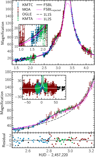
The light curve of this event, shown in Figure 1, looks very much like a single-lens event, except during the short time interval $\mathrm{HJD^{\prime}}\in[7,222.6,\,7,223.1]$, close to the peak of magnification. In this interval, the observations of the four observatories (MOA, KMTC, KMTA, and OGLE) caught a clear bump (the anomaly) in the light curve corresponding to a deviation from a single-lens model. This deviation typically occurs when the “major image” created by a host star is perturbed by the gravity of a companion, possibly a planet. This image moves in the vicinity of the lens Einstein ring during the lens-source relative motion, at an angular separation from the host star close to the angular Einstein radius,

$$\theta_{\mathrm{E}}=\sqrt{\frac{4GM}{c^{2}D_{\mathrm{S}}}\left(\frac{D_{\mathrm{S}}}{D_{\mathrm{L}}}-1\right)}\,,$$ (2)

where $G$ is the gravitational constant, $c$ is the speed of light, $M$ is the total mass of the lens, and $D_{\mathrm{L}}$ and $D_{\mathrm{S}}$ are, respectively, the observer-lens and observer-source distances. Consequently, such a perturbation is very likely when the companion is located close to the Einstein ring of the host star (Griest & Safizadeh, 1998). The single-lens model indicates a high-magnification event that is very sensitive to the detection of planets around the peak of magnification, i.e., when the multiple images created by the host are very much elongated around the Einstein ring. Hence, in this context, the anomaly is compatible with a source star that crosses a caustic.

We start modeling the light curve based on a point-source single-lens model (hereafter “1L1S”) that does not require any large computing power while providing a first estimate of the most fundamental parameters. During this process, we fit the event with a Paczyński light curve (Paczyński, 1986) that depends on three parameters: the impact parameter of the apparent source trajectory relative to the lens, $u_{0}$; the time at which the source reaches $u_{0}$, $t_{0}$; and the Einstein radius crossing time, $t_{\mathrm{E}}=\theta_{\mathrm{E}}/\mu_{\mathrm{rel}}$, where $\mu_{\mathrm{rel}}$ is the lens-source relative proper motion.

Three additional parameters are required to model a binary lens: the mass ratio of the secondary to primary lens component $q=M_{2}/M_{1}$, where $M_{2}$ ($M_{1}$) is the mass of the secondary lens (the mass of the primary lens, with $M=M_{1}+M_{2}$); the separation in Einstein units, $s$; and the angle between the lens axis and the source trajectory, $\alpha$. For a binary lens, $u_{0}$ is the distance of closest approach between the lens center of mass and the source. Due to the possibility that the lens crosses or approaches close to a caustic, we take into account the physical size of the source, i.e., the finite source effects, by adding one model parameter, namely, the source radius crossing time, $t_{\star}=\rho\,t_{\mathrm{E}}=\theta_{\star}/\mu_{\mathrm{rel}}$, where $\rho$ is the source angular radius in Einstein units, i.e.,

$$\rho=\frac{\theta_{\star}}{\theta_{\mathrm{E}}}\,,$$ (3)

with $\theta_{\star}$ the source angular radius. The source crossing time links the parameters used in the fit and two fundamental physical quantities: the angular Einstein radius and the lens-source relative proper motion. Hereafter, we refer to the resulting “finite-source binary-lens” model as “FSBL.”

Finite source effects in microlensing light curves are usually sensitive to the stellar limb darkening (Albrow et al., 1999; Cassan et al., 2006). We include this effect in the model by considering a source described as a nonuniform disk (An et al., 2002; Zub et al., 2011) with the linear intensity-normalized profile

$$I(r)=\frac{1}{\pi}\left[1-\Gamma\left(1-\frac{3}{2}\sqrt{1-r^{2}}\right)\right]\,,$$ (4)

where $\Gamma$ is a linear limb-darkening coefficient and $r$ is the fractional distance from the center toward the limb of the star (i.e., $r\in[0,1]$). The linear equation (4) is generally a good approximation, in particular when the limb darkening is weakly constrained, e.g., for a particularly faint event like OGLE-2015-BLG-1670. We use the extinction-free source color found in Section 4.1 to estimate the effective temperature of the source, $T_{\mathrm{eff}}\approx 4600\,\mathrm{K}$, and its surface gravity, $\log g\approx 4.5$. For these values and adopting a metallicity $\log[M/H]=0$, we adopt the linear limb-darkening coefficients $u_{I}=0.6155$ (i.e., $\Gamma_{I}=0.5163$) and $u_{R}=0.7259$ (i.e., $\Gamma_{R}=0.6384$; Claret & Bloemen, 2011).

Finally, two parameters describe the unlensed source flux: $f_{\mathrm{s},j,\lambda_{i}}$, for any observatory, $j$, and passband, $\lambda_{i}$, and the excess flux, $f_{\mathrm{b},j,\lambda_{i}}$, resulting from the combination of any (and possibly several) “blend” stars. The blend can be either the lens itself or an unrelated star or stars. At any time $t$, the total flux of the microlensing target is

$$F_{j,\lambda_{i}}(t)=A(t)f_{\mathrm{s},j,\lambda_{i}}+f_{\mathrm{b},j,\lambda_{i}}\,,$$ (5)

where $A(t)$ is the source flux magnification at the date $t$. During the fitting process, for each set of nonlinear fit parameters and each passband, we solve the linear equation (5) (Rhie et al., 1999). In practice, $\lambda_{i}$ is the $I$ and $R$ filters. The source magnitude reported in Table 2, $I_{\mathrm{S}}$, is derived after the OGLE-IV photometry calibration.

3.2 Exploration of Parameters Space

3.2.1 Single-source Binary-lens Model

The best-fit 1L1S model is used as a starting point to explore binary-lens models. Computing the source flux magnification for a high-magnification event is usually time-consuming. Several numerical methods have been developed to optimize the computational cost, such as image contouring methods (Gould & Gaucherel, 1997; Dominik, 2007; Bozza, 2010) or ray-shooting techniques (Bennett & Rhie, 1996; Dong et al., 2006, 2009). During the light-curve modeling process, we use the image-centered ray-shooting method (Bennett & Rhie, 1996). We start exploring possible FSBL solutions using the initial condition grid search method described in Bennett (2010) for $\log\left(0.3\right)\leqslant\log{s}\leqslant\log\left(12.5\right)$ and $-4\leqslant\log{q}\leqslant-0.954$. The three parameters $\{s,\,q,\,\alpha\}$ are fixed, while the other parameters vary. We use a Monte Carlo approach to perform a global search using a Metropolis algorithm with an adaptive size of the proposal function to find the best-fit models. For each model, we compute the $\chi^{2}$ value. The local minima of the $\chi^{2}$ function correspond to plausible physical models; we select the solutions with $\Delta\chi^{2}=\chi^{2}-\chi^{2}_{\mathrm{min}}\leqslant 150$ for a refined exploration that allows all parameters to vary during a Markov chain Monte Carlo (MCMC) to sample the posterior probability distribution.

Table 2: Parameters for the Best-fit Model and the Corresponding Statistical Values from the Posterior Probability Distribution Function

		Best Fit			MCMC (95.5% Confidence Interval)
Parameter	Units	$s<1$	$s>1$	$s>1$	$s<1$	$s>1^{\text{a}}$
$\chi^{2}$		7052.80000	7042.80000	7046.20000	$\cdots$	$\cdots$
$\Delta\chi^{2}$	$\cdots$	0010.00000	0000.00000	0003.40000	$\cdots$	$\cdots$
$q/10^{-4}$	$\cdots$	0001.12809	0000.79836	0000.89779	$1.50^{+0.86}_{-0.68}$	$1.00^{+0.40}_{-0.31}$
$s$	$\cdots$	0000.96318	0001.03529	0001.05331	$0.965\pm 0.010$	$1.056^{+0.028}_{-0.020}$
$t_{\mathrm{E}}$	days	0035.19112	0027.91693	0023.94770	$27.0^{+12}_{-7.5}$	$23.3^{+9.1}_{-5.2}$
$t_{\star}/10^{-2}$	days	0006.08626	0003.19663	0005.05031	$6.0\pm 1.1$	$5.05^{+0.60}_{-1.7}$
$t_{0}$	$\mathrm{HJD^{\prime}}$	7223.34497	7223.34246	7223.34247	$7223.3454\pm 0.0036$	$7223.3427\pm 0.0033$
$u_{0}/10^{-3}$	$\cdots$	0003.52282	0004.30742	0005.08333	$4.7^{+1.9}_{-1.5}$	$5.3^{+1.7}_{-1.5}$
$\alpha$	rad	0000.26894	0000.25528	0000.25522	$0.275^{+0.020}_{-0.024}$	$0.257^{+0.015}_{-0.013}$
$\rho/10^{-3}$	$\cdots$	0001.72949	0001.14505	0002.10889	$2.23^{+0.86}_{-0.71}$	$2.17^{+0.69}_{-1.0}$
$I_{\mathrm{S}}$	$\cdots$	0022.809	0022.540	0022.371	$22.51^{+0.40}_{-0.37}$	$22.34^{+0.40}_{-0.30}$

Notes. The uncertainties correspond to a 95.5% confidence interval, and the measurement is the median of the posterior. The parameter $\rho=t_{\star}/t_{\mathrm{E}}$ is not fit.

^a We include in this column the two degenerate solutions with $s>1$ because their two respective non-Gaussian posterior distributions are connected. As the volume of the parameter space that corresponds to a given confidence level is much larger in the vicinity of the solution with $s\approx 1.05$, the overall posterior probability close to that solution is higher. See discussion in Section 3.2.1.

Figure 2: Caustic topology of the two best-fit models ($s=1.03529$, top panel; $s=1.05331$, middle panel) and the corresponding degenerate solution ($s<1$, bottom panel), shown by the black line. The colored line refers to the source trajectory relative to the lens, and the inset shows a zoom-in on the caustic crossing. In the top panel, the source edge is drawn at $\mathrm{HJD^{\prime}}=7,221.375$, the time of the caustic entry ($\mathrm{HJD^{\prime}}=7,222.63$), and $\mathrm{HJD^{\prime}}=7,222.88$ (time of the peak of the planetary anomaly). In the middle and bottom panels, it is drawn at the time of the caustic entry ($\mathrm{HJD^{\prime}}=7,222.64$ and $7,222.62$, respectively) and $\mathrm{HJD^{\prime}}=7,222.88$ (same as the top). The color along the source trajectory refers to the magnification, and the arrow shows the direction of the source-lens relative motion. The caustic is shown in the center-of-mass reference frame, with the planet (the host star) on the left-hand side (right-hand side).

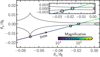
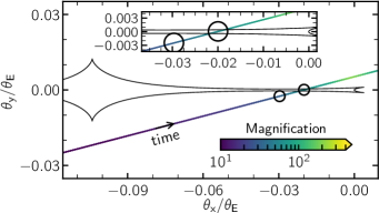
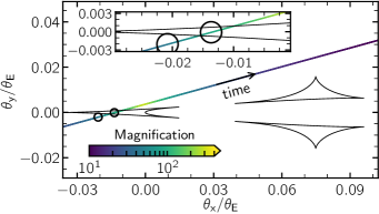
The best-fit models for this event have a planetary mass ratio. These planetary solutions are favored over a single-lens model by $\Delta\chi^{2}=932$. In particular, two main models (and their degenerate solutions) were identified during the refined exploration of the parameter space: one with $q=1.19\times 10^{-3}$, which is ruled out by $\Delta\chi^{2}\approx 109$, compared to the best-fit model with $q=7.98357\times 10^{-5}$. The best-fit model parameters are presented in Table 2 and the model light curves are plotted in Figure 1 (hereafter the “FSBL model”). As we can see in this figure, the best-fit model provides a better explanation for both the caustic entry and the anomaly than the higher mass-ratio solution (hereafter the “$\mathrm{FSBL_{rejected}}$ model”). Note that we have chosen the FSBL model as a reference in Figure 1; i.e., we plot the corrected magnification,

$$A_{i,\mathrm{plot}}(t)=\frac{f_{\mathrm{s},i}}{f_{\mathrm{s,ref}}}A_{i}(t)+\frac{f_{\mathrm{b},i}-f_{\mathrm{b,ref}}}{f_{\mathrm{s,ref}}}\,,$$ (6)

where $A_{i}$ is the magnification derived for the model $i=\{\mathrm{FSBL_{rejected},1L1S,1L2S}\}$, $f_{\mathrm{s},i}$ and $f_{\mathrm{b},i}$ are the source and blend flux for the model $i$, and $f_{\mathrm{s,ref}}$ and $f_{\mathrm{b,ref}}$ are the calibrated source and blend flux derived from the reference model. The best-fit model describes an intermediate binary configuration (resonant caustic with $s=1.03529$ and $q=7.98357\times 10^{-5}$) shown in the top panel of Figure 2. The source trajectory passes close to the host star, responsible for the high-magnification values. Also, the caustic crossing happened in one of the thinnest regions of the caustic (slightly thinner than the source size), resulting in a moderate deviation from a single-lens model as shown in Figure 1. The magnification derived from the best-fit model reaches $A_{\mathrm{max}}\approx 232$. This solution also includes a cusp approach before the source crosses the caustic and during a gap in the observations at $\mathrm{HJD^{\prime}}\approx 7,221.4$ (see upper inset in Figure 1).

This best-fit model is degenerate with another slightly different solution characterized by $s=1.05331$ and $q=8.97794\times 10^{-5}$, disfavored by only $\Delta\chi^{2}=3.4$. As shown in Table 2, this solution has a higher source crossing time and slightly shorter Einstein timescale, resulting in a source radius approximately twice as large as the value derived from the best-fit model ($\rho=2.1\times 10^{-3}$ versus $1.1\times 10^{-3}$). The caustic topology and source trajectory are similar to the best-fit model and are shown in the middle panel of Figure 2. The source crosses a resonant caustic in a region where the distance between the two caustic edges is smaller than the source radius. The degeneracy between the two solutions with $s>1$ is due to a degeneracy between the source size and the width of the caustic that occurs when the anomaly consists of a smooth “bump.”

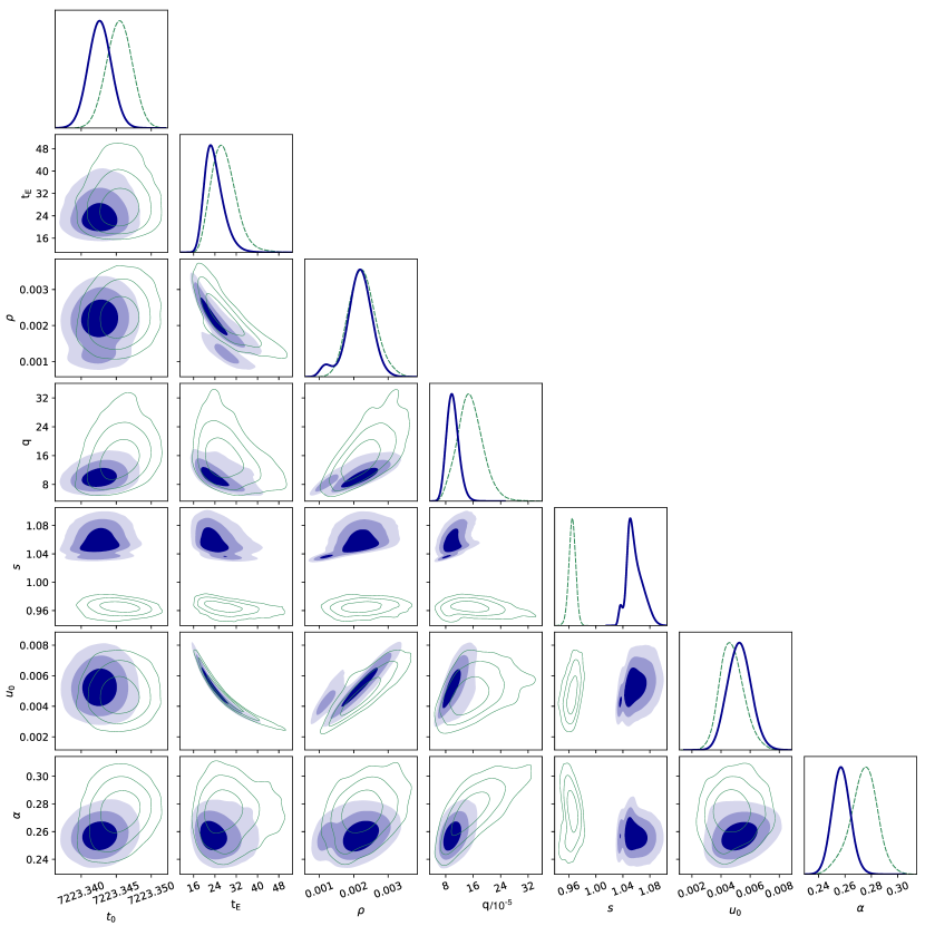
These caustic crossing features can be approximately reproduced by a close binary-lens configuration with $s=0.96318$ and $q=1.128086\times 10^{-4}$, as shown in the bottom panel of Figure 2. This solution corresponds to the well-known $s\leftrightarrow 1/s$ degeneracy (Griest & Safizadeh, 1998; Dominik, 1999), which is common when a caustic crossing involves the central caustic in a close binary-lens configuration. For a planetary mass ratio, the closer $s$ is to 1, the weaker the degeneracy. As the lens parameters are very close to $s=1$, it is possible to choose between the $s<1$ and $s>1$ solutions: the latter is favored by $\Delta\chi^{2}=10.0$. For $s<1$, we do not find two likelihood maxima. Conversely, all of the MCMC chains converged to the same solution shown in Table 2 and characterized by a source size of $\rho=1.73\times 10^{-3}$. The two $s<1$ and $s>1$ degenerate solutions are very close in terms of goodness of fit, and the marginal distributions derived at the end of the MCMC are very much overlapping for all of the parameters except the separation, $s$. The parameter correlation and marginal distributions for both solutions are shown in Figure 3. The solution corresponding to $s=1.05331$ is a local maximum of the likelihood, i.e., one mode of the posterior distribution. The $\Delta\chi^{2}$ between these two solutions with $s>1$ corresponds to a relative probability of $0.18$. However, because the volume of the parameter space that corresponds to a given confidence level is much larger in the vicinity of the solution with $s\approx 1.05$, the overall posterior probability close to that solution is higher. For the next stages of the analysis, we use the full multimodal posterior to estimate the lens mass and distance in Section 4.2, including the solution with $s<1$, rather than selecting the best-fit model only.

Figure 3: Correlation between the parameters for the best-fit model ($s>1$) in blue and its degenerate alternative ($s<1$) in green (see Section 3.2). For each solution, the three shaded areas (or contours) show the $68.3\%$, $95.5\%$, and $99.7\%$ confidence regions, respectively, from the darkest to lightest color. The two solutions with $s>1$ are included in the blue shaded regions. The units are defined in Table 2.

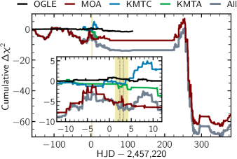
We also searched for a possible parallax detection in the light curve. During this event, the Earth’s instantaneous acceleration in the heliocentric reference frame projected to the lens plane was only $\approx 50\%$ of its maximum. Indeed, the peak of magnification was reached on 2015 July 19, less than a month after the minimum of the Earth’s acceleration perpendicular to the line of sight. Additionally, this event is faint, and the uncertainties make it more difficult to detect asymmetric features in the light-curve tails. The best-fit model with parallax is favored over the static model by $\Delta\chi^{2}=54$. This model has a secondary magnification peak during the gap between the 2015 and 2016 observing seasons. The upper panel of Figure 4 shows the cumulative $\Delta\chi^{2}$ between the model including parallax compared to the best-fit static solution. As we can see in this figure, the overall $\chi^{2}$ improvement mostly comes from baseline observations performed by MOA during the 2016 observing season ($7470\leqslant\mathrm{HJD^{\prime}}\leqslant 7500$), likely due to fluctuation in the baseline data. Out of the overall $\chi^{2}$ improvement of $54$, there is an improvement of only $\Delta\chi^{2}\approx 6$ for $\mathrm{HJD^{\prime}}\leqslant 7231$, mostly due to data points from MOA and KMTA: the improvement is, respectively, $\Delta\chi^{2}\approx 4.4$ and $1.7$ for observations when the magnification is $A\geq 3.5$ (the noise in magnification is typically $\pm 2.5$). Meanwhile, numerous data points from KMTC favor the static model by $\Delta\chi^{2}\approx 5$ during the same time interval. We conclude that the overall improvement when the magnification emerges from the noise in the baseline is $\Delta\chi^{2}\leqslant 0.5$. In summary, $90\%$ of $\chi^{2}$ improvement for the model with parallax comes from baseline data, when the magnification is $A\leqslant 1.03$, and the remaining $10\%$ is due to data points at low magnification and brightness (the target brightness is $I\approx 19.3$ when $A=10$). For these reasons, we do not claim a parallax detection in the light curve of this event. As a consequence, an absolute mass measurement of the lens OGLE-2015-BLG-1670L components will not be possible with the light-curve data alone, but the high precision on the planet-to-host mass ratio will be enough to identify the physical nature of the planetary component (see Section 4).

Figure 4: Cumulative $\Delta\chi^{2}$ for the single-source, binary-lens model with parallax (upper panel) and the binary-source, single-lens model (lower panel). The best-fit planetary model in Table 2 is used as a reference in both cases. The yellow shaded region corresponds to the time interval shown in the upper panel of Figure 1, and the dotted lines indicate the region where the magnification is substantially different than that of a single-source, single-lens model ($7222.4<\mathrm{HJD^{\prime}}<7223.22$).

3.2.2 Binary-source Single-lens Model

Table 3: Parameters for the best-fit 1L2S Including the Source Orbital Motion

Parameter	Units	Value
$\chi^{2}$	$\cdots$	7137.40000
$\Delta\chi^{2}$	$\cdots$	0094.60000
$t_{\mathrm{E}}$	days	0006.73528
$t_{0}$	$\mathrm{HJD^{\prime}}$	7223.35787
$u_{0}/10^{-3}$	$\cdots$	0020.09699
$t_{0,2}$	$\mathrm{HJD^{\prime}}$	7222.89358
$u_{0,2}/10^{-3}$	$\cdots$	0008.21605
$f_{s_{2},I}/10^{-2}$	$\cdots$	0003.71410
$f_{s_{2},R}/10^{-2}$	$\cdots$	0003.95530
$dt_{\mathrm{E},2}$	days	0001.80657
$10^{-2}/T_{\mathrm{Sorb}}$	days-1	0006.60615

In the previous section, we have described the modeling strategy we followed to find the binary-lens model that best fits the light curve. For completeness, we also consider possible binary-source, single-lens models (hereafter called 1L2S), starting with a grid search method for the source projected separation in Einstein units, $s_{\mathrm{source}}$ (300 points for $10^{-3}\leqslant s_{\mathrm{source}}\leqslant 1$, and 100 points for $1\leqslant s_{\mathrm{source}}\leqslant 5$). To explore 1L2S models, we use the binary-source, binary-lens modeling code written to model microlensing event MOA-2010-BLG-117 (Bennett et al., 2018). This code uses the single-lens parameters $t_{0,i}$, $u_{0,i}$, and $t_{\mathrm{E},i}$, corresponding to the microlensing of the stellar binary component $i=\{0,1\}$.

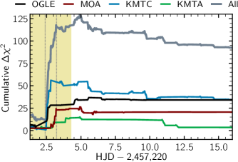
To include the orbital motion of the binary source, we introduce $\mathrm{d}t_{\mathrm{E}}=t_{\mathrm{E},2}-t_{\mathrm{E},1}$ to account for the different lens-source relative motions due to this source’s orbital motion in the direction parallel to the source-lens relative motion. The orbital motion perpendicular to the source motion can be described by the difference in the angles that the source-lens relative motion subtends with respect to the lens system, $d\theta$. However, because of the circular symmetry of a single-lens system, neither these angles nor their difference is measurable. However, when allowing for a circular orbit with period $T_{\mathrm{Sorb}}$, as in Bennett et al. (2018), we do need $d\theta$ to describe the instantaneous velocity of the two sources, although the angle, $\theta$, remains unmeasurable for a single-lens system. We use $1/T_{\mathrm{Sorb}}$ as our parameter to describe the orbital period. The reference time when the sources are at their reference positions and velocities is $\mathrm{HJD^{\prime}}=7223.335$. We use the parameters $t_{\mathrm{E},1}$ and $dt_{\mathrm{E}}$ instead of the two independent Einstein timescales. In order to avoid unphysical regions of the parameter space, we impose the condition that the source 2–to–source 1 flux ratio must be the same for all data sets taken in the same passband. Thus, we fit two parameters, $f_{s2,I}$ and $f_{s2,R}$, one for each filter used to obtain the data. We have explored the parameter space using an MCMC algorithm, and we find that the best binary-lens model is favored over the best binary-source model by $\Delta\chi^{2}=95$. The best-fit 1L2S model parameters are shown in Table 3, and the lower panel of Figure 4 is the cumulative $\Delta\chi^{2}$ between the 1L2S binary-source model. Figure 4 indicates that the binary-lens model is highly favored by $\Delta\chi^{2}\approx 95$. In particular, $\Delta\chi^{2}\approx 115$ arises from a time window corresponding to the anomaly. As a consequence, a 1L2S model does not compete with the binary-lens alternatives presented in Table 2.

3.2.3 Robustness of Best-fit Solutions

The error-bar normalization law adopted in equation (1) might be sensible and is standard practice when dealing with DIA photometry. In the case of OGLE-2015-BLG-1670, we investigate the effect of a moderate change of $e_{\mathrm{min}}$ on the robustness of the best-fit solutions reported in Table 2. We consider the five following situations:

1. $e_{\mathrm{min}}(\text{all})=0$;

2. $e_{\mathrm{min}}(\text{KMTA, KMTC})=0$, $e_{\mathrm{min}}(\text{others})=0.003$;

3. $e_{\mathrm{min}}(\text{KMTA})=0$, $e_{\mathrm{min}}(\text{others})=0.003$;

4. $e_{\mathrm{min}}(\text{KMTC})=0$, $e_{\mathrm{min}}=0.003$ otherwise; and

5. $e_{\mathrm{min}}(\text{KMTA})=0$, $e_{\mathrm{min}}(\text{KMTC})=0.006$, $e_{\mathrm{min}}(\text{others})=0.003$.

In each case, we compute $k$ so that $\chi^{2}_{\mathrm{red}}=1$, and we run several MCMCs from the plausible physical models identified after the grid search, following the same method as described in Section 3.2. The resulting best-fit models are very close to the ones originally identified. Then, we run refined MCMCs from these models. At this stage, we find solutions within $1\sigma$–$2\sigma$ of the model parameters reported in Table 2 and 3. Finally, we run a last set of MCMCs using the parameters from Table 2 and 3 as initial conditions.

As expected, we find a slightly different $\chi^{2}$ difference between each model. However, the best-fit parameters do not change, and this very limited change in the $\chi^{2}$ difference shows that the conclusions do not depend on the fine details of the coefficients used in the error-bar normalization law assumed. First, the high mass ratio model ($q\sim 1.2\times 10^{-3}$) remains disfavored by a $\chi^{2}$ difference greater than 100 in all cases. Second, the 2L1S low mass ratio solution is highly favored by $\Delta\chi^{2}>96$ compared to the 1L2S model in all cases. Finally, regarding planetary solutions, the most significant difference is obtained in case 4: $\chi^{2}(s=1.05)-\chi^{2}(s=1.03)=2.36$, and $\chi^{2}(s<1)-\chi^{2}(s=1.03)=9.10$. The change in the $\chi^{2}$ difference remains very small, and in that particular case, KMTC error bars are assumed to be smaller than they should be. Conversely, the less significant changes are found in case 5, where $e_{\mathrm{min}}$ is assumed to be twice the value originally chosen.

We conclude that the best-fit model parameters are robustly determined, and the results are not too sensitive to a moderate change of the error-bar normalization coefficients. The overlap of observations from multiple surveys partly explains this robustness. Indeed, the data from the four surveys cover the anomaly but also many portions of the light curve. For instance, OGLE, MOA, KMTC, and KMTA observed during the event, at the anomaly, and at the baseline. Similarly, OGLE, MOA, and KMTC have numerous simultaneous observations when the magnification is high.

4 Lens Physical Properties

4.1 Measurement of the Angular Einstein Radius

The measurement of the angular Einstein radius provides one relation between the lens mass and distance. Indeed, from equation (2), the lens total mass reads

$$M=\frac{c^{2}\,\theta_{\mathrm{E}}^{2}}{4G}\left(\frac{1}{D_{\mathrm{L}}}-\frac{1}{D_{\mathrm{S}}}\right)^{-1}\,.$$ (7)

Modeling the microlensing light curve yields a precise measurement of $\rho$, as well as the source flux. By combining the latter quantity with a color-magnitude diagram (CMD) of stars from the same field of view as the target, it is possible to measure the source color and determine its angular radius, $\theta_{\star}$.

The first step of the source characterization is to calibrate the instrumental MOA-II magnitudes, $R_{\mathrm{MOA}}$ and $V_{\mathrm{MOA}}$, by a cross-referencing of stars from the MOA-II dophot catalog with stars in the OGLE-IV catalog. We use these stars to build a catalog with magnitudes in the standard Kron–Cousins $I$ and Johnson $V$ passbands (Udalski et al., 2015). This calibration is required because the OGLE-IV field “BLG500.20” has not been observed by OGLE-III, and there was no observation magnified enough in the $V$ band to derive the source color. A total of 881 stars from the OGLE catalog and within a 2′ circle centered on the source are cross-matched with the 167 stars extracted from the same field of view and observed by MOA. From this, we select stars from the red giant branch to derive the following relation between the MOA-II instrumental magnitude and the standard magnitudes and colors (Gould et al., 2010a):

$$R_{\mathrm{MOA}}-I=(0.000\pm 0.053)+(0.161\pm 0.011)\left(V-I\right)\,.$$ (8)

Equation (8) is derived using only the nine cross-referenced stars found in the red branch in both the MOA and OGLE catalogs. The instrumental color-color relation, along with the calibrated OGLE CMD, is shown in Figure 5.

Figure 5: The upper panel shows the $(V-I,I)$ CMD in the standard Kroni–Cousins $I$ and Johnson $V$ photometric systems of OGLE-IV stars within $2\arcmin{}$ around the source (black dots), not corrected for the interstellar extinction. The red circle indicates the RCG centroid, the blue dot indicates the source magnitude and color for $s>1$, and the black open circle corresponds to the solution $s<1$ (the uncertainties are comparable to the case $s>1$). The green dots show the Hubble Space Telescope CMD from Holtzman et al. (1998) shifted to the bulge distance and extinction derived in Section 4.1 for the OGLE-2015-BLG-1670 line of sight. The lower panel shows the empirical color-color transformation between the standard photometric system and the instrumental color $(R_{\mathrm{MOA}}-I_{\mathrm{OGLE}})$. The gray shading indicates the 99% confidence interval, and the red circles show the outliers for $(V-I)>3$.

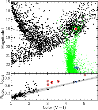
The CMD plotted in Figure 5 reveals a difference in color of $\gtrsim 3$ between stars from the red giant branch and the main-sequence stars from the blue plume. It is consistent with a field that suffers from dust distributed along the line of sight, with the bluer stars further away from the Galactic bulge than the redder stars. It is particularly visible when comparing the Hubble Space Telescope (HST) CMD from Holtzman et al. (1998), shifted to the extinction of the red clump giant (RCG) in Figure 5. The event OGLE-2015-BLG-1670 lies in a high-extinction region of the Milky Way, at a low $|b|$ ($b=-1\fdg 12048$), in a field that could be observed by WFIRST. In the optical $I$ and $V$ passbands, the extinction is more severe than in the NIR, resulting in a sparse CMD in Figure 5, mostly because the brightness in the $V$ passband could not be measured for many stars. Extracting the photometry of the faintest stars is one challenging task, especially in the $V$ band and for targets with $I\gtrsim 21$. In particular, the blue stars indicated by the black dots in Figure 5 and with $I>21$, are likely suffering from systematic errors, and we reject them in our analysis.

The next step is to measure the extinction and reddening of stars close to the source and find its color. We use two independent methods to find the location of the RCG. On the one hand, a nonparametric kernel distribution estimation method identifies a local maximum of the two-dimensional probability distribution function in the red giant branch due to the RCG stars. This method yields a color $(V-I)_{\mathrm{RCG}}=4.51\pm 0.15$ and a magnitude $I_{\mathrm{RCG}}=17.93\pm 0.28$. On the other hand, the centroid of the RCG stars is $(V-I)_{\mathrm{RCG}}=4.54\pm 0.02$ and $I_{\mathrm{RCG}}=18.05\pm 0.1$. While the two methods do not provide the same uncertainties, the results are compatible. Moreover, we test the reliability of this measurement by searching for the centroid of the RCG stars located within a $1\arcmin$ circle (instead of $2\arcmin$) centered on the source. We find $(V-I)_{\mathrm{RCG}}=4.54\pm 0.03$ and $I_{\mathrm{RCG}}=18.02\pm 0.2$. These values are well within the error bars of the previous measurement, thus indicating that the RCG location can be accurately measured despite the high extinction.

For a source located in the Galactic bulge, the absolute magnitude and color of the RCG are $M_{I,\mathrm{RCG}}=-0.17\pm 0.05$ (Chatzopoulos et al., 2015; Nataf et al., 2016) and $(V-I)_{\mathrm{RCG},0}=1.06$ (Bensby et al., 2013). The distance to the RCG can be derived from the measurement of the distance to the Galactic center (Nataf et al., 2016), $D_{\mathrm{GC}}=8.33\,\mathrm{kpc}{}$,

$$D_{\mathrm{RCG}}=\frac{D_{\mathrm{GC}}\sin{(\phi)}}{\cos{(b)}\sin{\left(l+\phi\right)}}\,,$$ (9)

where $\phi=40^{\circ}$ is the angle between the Galactic bulge major axis and the line of sight of the Sun. For OGLE-2015-BLG-1670, we find the RCG to be at a distance of $D_{\mathrm{RCG}}=8.14\,\mathrm{kpc}{}$, corresponding to a distance modulus of $\mu=14.55$. If we assume that the source suffers from the same extinction and reddening as the RCG (i.e., the source is assumed to be in the Galactic bulge, at $8.14\,\mathrm{kpc}$ from Earth), the dereddened source magnitude is $I_{\mathrm{s,0}}=I_{\mathrm{s}}+M_{I,\mathrm{RCG}}+\mu-I_{\mathrm{RCG}}$, i.e., $I_{\mathrm{s,0}}=18.68^{+0.20}_{-0.19}$, and for $(V-I)_{\mathrm{s}}=4.59^{+0.14}_{-0.13}$, we find $(V-I)_{\mathrm{s,0}}=1.11^{+0.14}_{-0.13}$. These values correspond to an extinction $A_{I}=3.67$ (in good agreement with the $A_{I}=3.5$ derived from Gonzalez et al. (2012) after the transformation from the NIR to the I band), a color excess $E(V-I)=3.48$, and a reddening $R_{V,I}=A_{V}/E(V-I)=2.05$. In this section, we use the source brightness and color derived from the solution $s>1$ in Table 2 in order to explain the method. However, we include all of the degenerate solutions in the final derivation of the lens properties (see Section 4.2).

As expected from the visual inspection of Figure 5, this field has a high extinction. Despite the difficulty of detecting events at a low $\left|b\right|$ with optical microlensing surveys, a few events have already been observed in this region (see Section 1). Although the extinction substantially varies at a subdegree angular scale, we have compared the extinction to the values derived for OGLE-2013-BLG-1761, the closest planetary event ($(l,b)=(0.9368\arcdeg,-1.4842\arcdeg)$). The analysis of this event yields $E(V-I)=1.87$ and $A_{I}=1.95$ (Hirao et al., 2017). Although the extinction is lower, the reddening coefficient $R_{V,I}=2.04$ is consistent with the value we find. For comparison, in the Baade window, Stanek (1996) found a reddening coefficient $R_{V,I}=A_{V}/E(V-I)=2.49$, a value broadly consistent with our measurement despite the higher extinction in the line of sight for OGLE-2015-BLG-1670. Also, from the extinction maps built from the OGLE-III catalog (Nataf et al., 2013), OGLE-2015-BLG-1670 lies in a region with $E(V-I)\geq 1.34$, as expected. Finally, for the Galactic coordinates $(0.5,-1.8)$, extrapolating the empirical law predicting the red clump magnitude (Nataf et al., 2013) beyond its scope, we find a value $I_{\mathrm{RC}}=18.18$, consistent with our measurement.

The last step is deriving the angular source size from the following empirical relation (Boyajian et al., 2014),

$$\log\left(\frac{2\theta_{\star}}{\mathrm{mas}}\right)=0.501414-0.2I_{\mathrm{s,0}}+0.419685(V-I)_{\mathrm{s},0}\,,$$ (10)

inferred from stars with colors corresponding to $3900<T_{\mathrm{eff}}<7000$ (Bennett et al., 2017). We find that the angular source size $\theta_{\star}=0.85^{+0.14}_{-0.12}\,\mu\mathrm{as}$, with error bars mostly due to the uncertainty on the source color and brightness rather than the 2% uncertainty on equation (10). The source color is consistent with a K2–K4 main-sequence star, with an effective temperature $T_{\mathrm{eff}}\approx 4600\,\mathrm{K}$.

Table 4: Lens and Source Properties Derived from the Solutions $s<1$ and $s>1$
and the Bayesian Analysis Described in Section 4.2

Parameter	$s<1$	$s>1$	Bayes	Units
Einstein radius $\theta_{\mathrm{E}}$	$0.392^{+0.077}_{-0.062}$	$0.395^{+0.084}_{-0.061}$	$0.382^{+0.087}_{-0.076}$	$\mathrm{mas}$
Lens-source proper motion $\mu_{\textrm{rel,G}}$	$5.4^{+1.1}_{-0.9}$	$6.21^{+1.2}_{-0.95}$	$6.0\pm 1.2$	$\mathrm{mas}\,\mathrm{yr}^{-1}$
Source magnitudea $I_{\mathrm{S,0}}$	$18.85\pm 0.22$	$18.68^{+0.20}_{-0.19}$	$18.66\pm 0.20$	$\cdots$
Source colorb $(V-I)_{S,0}$	$1.21\pm 0.14$	$1.11^{+0.14}_{-0.13}$	$1.11\pm 0.14$	$\cdots$
Source angular radius $\theta_{\star}$	$0.87^{+0.16}_{-0.13}$	$0.85^{+0.14}_{-0.12}$	$0.85^{+0.14}_{-0.12}$	$\mu\mathrm{as}$

Notes.

^a $I$-band dereddened source magnitude.

^b Corrected for reddening.

The combination of the measurement of $\theta_{\star}$ and Equation (3) yields the Einstein angular radius for the best-fit model, $\theta_{\mathrm{E}}=0.395^{+0.084}_{-0.061}\,\mathrm{mas}$. Hence, the lens-source relative proper motion in the geocentric reference frame is $\mu_{\textrm{rel,G}}=6.21^{+1.2}_{-0.95}\,\mathrm{mas}\,\mathrm{yr}^{-1}$. The main results from this section are summarized in Table 4. This table includes the two degenerate solutions, $s>1$ and $s<1$, and shows that they yield measurements that are consistent with each other.

4.2 Lens Properties

Equation (7) is one relation between the lens mass and distance. As we could not measure the microlens parallax, the lens mass cannot be directly derived from the light-curve modeling. However, all lens configurations are not equally probable. We combine the microlensing light-curve analysis with a Galactic model in a Bayesian framework to quantify the relative probability between the different solutions and find the physical properties of the lens system.

Figure 6: Posterior probability distribution of the lens properties from a Bayesian analysis that includes the two degenerate solutions with $s>1$ and $s<1$ from Section 3.1, weighted by the Galactic model priors described in Section 4.2. Two shaded areas are separated by a blue line. They show the contribution of the thin and thick disk (light gray), and the spheroid and bulge (dark gray) to the posterior distribution (black line). The black vertical solid line indicates the median of the distribution, while the dotted-dashed and dotted lines respectively show the $68.3\%$ and $95\%$ confidence intervals.

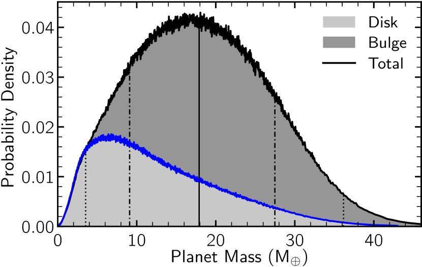
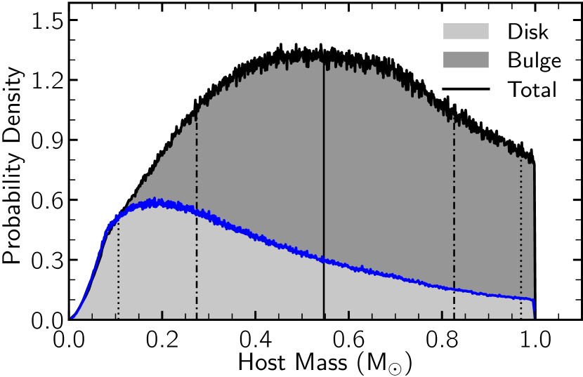
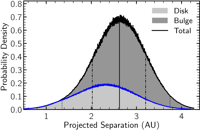
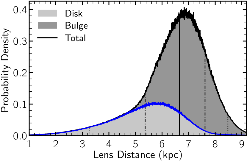
We use the same Galactic model as described in Bennett et al. (2014) based on stellar densities from Robin et al. (2003) with truncated escape velocities. This model includes a barred bulge, a spheroid, a thin disk and a thick disk. This model assumes that, for any given Einstein radius and mass ratio, the probability for a star to host a planet does not depend on the host mass. At this stage, we include all degenerate models found in Section 3.1 (solutions with $s>1$ and $s<1$). As shown in Figure 3, the posterior probability distributions of each local minimum have similar statistical properties. Consequently, we weight each Markov chain by the $\chi^{2}$ difference between their corresponding best-fit models.

Figure 6 shows the probability distribution of the lens properties resulting from this Bayesian analysis. As the two degenerate solutions yield relatively close posterior distributions, these two solutions do not imply multimodal distributions. As expected, the lens mass and distance are not well constrained, and the Galactic priors largely drive the posterior distributions. The source flux measurement does not exclude main-sequence stars with a mass larger than $1\,M_{\sun}$, mostly because of the high extinction. However, such stars are rare in the Galactic bulge, and we use an upper limit for the lens mass equal to $1\,M_{\sun}$, as shown in Figure 6. The secondary lens component is found to be $17.9^{+9.6}_{-8.8}\,M_{\oplus}$, which is consistent with a Uranus- or Neptune-mass planet orbiting a primary lens component with a projected separation $2.62^{+0.58}_{-0.60}\,\mathrm{au}$. If we assume a circular planetary orbit with random orientation in space, the three-dimensional orbit radius is expected to be $3.2^{+1.8}_{-0.8}\,\mathrm{au}$. This planet is, therefore, orbiting its host well beyond the snow line. Besides, the host mass derived from this analysis cannot provide an unambiguous stellar type with an estimated mass $0.55\pm 0.28\,M_{\sun}$, consistent with an M dwarf or a solar-type star. With a lens-source proper motion of $\mu_{\textrm{rel,G}}=6.0\pm 1.2\,\mathrm{mas}\,\mathrm{yr}^{-1}$ in the geocentric reference frame and a lens distance $D_{\mathrm{L}}=6.7^{+1.0}_{-1.3}\,\mathrm{kpc}$, the lens may be either in the disk or in the bulge. In Figure 6, the light gray shading indicates the thin and thick disk contribution to the posterior distribution (black solid curve), while the dark gray shading indicates the spheroid and bulge contribution. Although these density profiles raise the possibility of a lens lying in the disk, they also suggest that a bulge lens is slightly more likely. The results of the Bayesian analysis are summarized in Tables 4 and 5.

Table 5: Physical Properties of the Lens OGLE-2015-BLG-1670L Derived from the Bayesian Analysis Described in Section 4.2

Parameter	Bayes	Units
Host mass $M_{1}$	$0.55\pm 0.28$	$M_{\sun}$
Planet mass $M_{2}$	$17.9^{+9.6}_{-8.8}$	$M_{\oplus}$
Projected separation $a_{\perp}$	$2.62^{+0.58}_{-0.60}$	$\mathrm{au}$
Deprojected separation $a$	$3.2^{+1.8}_{-0.8}$	$\mathrm{au}$
Lens distance $D_{\mathrm{L}}$	$6.7^{+1.0}_{-1.3}$	$\mathrm{kpc}$
Predicted lens magnitude $J_{l}$	$22.0^{+1.3}_{-1.7}$	$\cdots$
Predicted lens magnitude $H_{l}$	$20.8^{+1.3}_{-1.6}$	$\cdots$
Predicted lens magnitude $K_{s,l}$	$20.3^{+1.3}_{-1.5}$	$\cdots$

5 Summary and Discussion

Figure 7: Distribution of known exoplanet masses relative to the semi-major axis divided by the snow-line position at $a_{\mathrm{snow}}=2.7\,\mathrm{au}\,M_{1}/M_{\sun}$. Microlensing discoveries with direct host star and planet mass measurements are indicated with filled red circles. OGLE-2015-BLG-1670Lb corresponds to the thick black circle. Each planet from our solar system is indicated by its initial (except Mercury). Exoplanets not detected using microlensing are from the catalog http://exoplanet.eu/ (Schneider et al., 2011).

We have presented the analysis of the high-magnification ($A_{\mathrm{max}}\approx 230$) microlensing event OGLE-2015-BLG-1670. The anomaly is consistent with a binary lens with a planet-to-host mass ratio of $q\approx 10^{-4}$. There are two solutions to the event. The best has a planet-to-host mass ratio $q=1.00^{+0.18}_{-0.16}\times 10^{-4}$ and a projected separation $s=1.0556^{+0.015}_{-0.0087}$. The second solution has $q=1.50^{+0.39}_{-0.35}\times 10^{-4}$ and $s=0.9650\pm 0.0050$ but is disfavored by $\Delta\chi^{2}=10$. While we did not detect any reliable parallax signal in the light curve, the source caustic crossing constrains the angular source size, $\rho$, in Einstein units. Building the CMD from stars close to the target, we measured the RCG position and derived the dereddened source magnitude for the $s>1$ solution, $I_{s,0}=18.68^{+0.20}_{-0.19}$, and color, $(V-I)_{s,0}=1.11^{+0.14}_{-0.13}$, as well as an estimation of the source angular size, $\theta_{\star}=0.784^{+0.093}_{-0.13}\,\mu\mathrm{as}$. The source size serves as a “length calibration ruler” and yields the Einstein angular radius, $\theta_{\mathrm{E}}=0.395^{+0.084}_{-0.061}\,\mathrm{mas}$. The values for the $s<1$ solution are similar (see Table 4).

This lens mass ratio is very close to the break and the possible peak in the mass-ratio function identified recently for the first time (Suzuki et al., 2016) after combining MOA survey observations with previous statistical investigations (Gould et al., 2010b; Sumi et al., 2010; Cassan et al., 2012) to build the largest sample of microlensing planets in a study of the planets’ demography. For a mass ratio $q<q_{\mathrm{br}}$, the planet frequency is rising as $\mathrm{d}^{2}N/(\mathrm{d}\log{q}\times\mathrm{d}\log{s})=0.95\times(q/q_{\mathrm{br}})^{2.6}\,s^{0.46}$, whereas for $q_{\mathrm{br}}<q$, the planet frequency is dropping as $\mathrm{d}^{2}N/(\mathrm{d}\log{q}\times\mathrm{d}\log{s})=0.95\times(q/q_{\mathrm{br}})^{-0.85}\,s^{0.46}$, where $q_{\mathrm{br}}=0.67^{+0.90}_{-0.18}\times 10^{-4}$ is the mass-ratio function break that translates into 1 Neptune mass ($M\approx 20M_{\oplus}$) by assuming that M dwarfs dominate the microlensing planet host sample. A similar peak in the mass function around $M=6\,M_{\oplus}$ has been identified in a sample of Kepler planets orbiting M dwarfs (host stars that dominate the microlensing planet sample) detected by Kepler, but for shorter-period orbits (Dressing & Charbonneau, 2015). A recent exploration of the low-mass end of the mass-ratio function has also confirmed the turnover in the microlensing planet mass function (Udalski et al., 2018). However, the exact value of the mass-ratio break $q_{\mathrm{br}}$ is not well constrained due to a lack of planet detections in the regime $q<q_{\mathrm{br}}$. In this respect, OGLE-2015-BLG-1670L is a noteworthy detection that will tighten constraints on the lower end of the mass-ratio function.

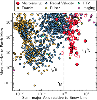
The measurement of $\theta_{\mathrm{E}}$ only partially solves the lens mass–distance degeneracy. However, it is possible to infer the lens physical properties by conducting a Bayesian analysis that combines the light-curve modeling with priors on the lens-source relative proper motion from a Galactic model. The resulting lens consists of a $17.9^{+9.6}_{-8.8}\,M_{\oplus}$ Neptune-mass planet orbiting a $0.55\pm 0.28$ main-sequence star with a projected orbital separation $2.62^{+0.58}_{-0.60}\,\mathrm{au}$. OGLE-2015-BLG-1670Lb is shown in Figure 7 as a thick black circle, together with the distribution of known exoplanets in mass versus semi-major axis divided by the location of the snow line, $a_{\mathrm{snow}}$. The location of the snow line in a protoplanetary disk depends on many parameters, including the host star properties (age, effective temperature, mass) and its environment (dust, gas, disk; e.g., see Ida & Lin, 2005; Kennedy & Kenyon, 2008; Min et al., 2011). Its dependency with the host star mass is often assumed to be a power law and scaled to its current position in the solar System: $a_{\mathrm{snow}}=2.7\,\mathrm{au}\,(M/M_{\odot})^{\alpha}$, with $\alpha=2$ for main-sequence stars whose mass is $0.2\,M_{\sun}<M<1.5\,M_{\sun}$ and optically thin disks (Ida & Lin, 2005), or in the range $[6/9\mathbin{;}8/9]$ (Kennedy & Kenyon, 2008) for hosts with $M<3\,M_{\sun}$, depending on the accretion rates and model assumptions. For consistency with previous articles reporting new microlensing detections, we adopt a linear law, i.e., $\alpha=1$. In Figure 7, exoplanets with a direct mass measurement are indicated by filled red circles, whereas open red circles show the planets whose masses have been derived from Galactic models. OGLE-2015-BLG-1670Lb lies well beyond the snow line.

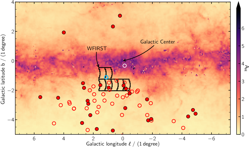
High-resolution follow-up would help in measuring the actual mass of the planet in the future, either by resolving the source and the lens or by a measurement of the excess flux on top of the source. Following the same reasoning as in Section 4.2, we use our Galactic model to predict the lens brightness in the three passbands. For an extinction $A_{J}=1.60$, $A_{H}=0.99$, and $A_{K_{s}}=0.65$ (Gonzalez et al., 2012), we estimate the lens magnitude to be $J_{l}=22.0^{+2.7}_{-2.6}{}$, $H_{l}=20.8^{+2.7}_{-2.3}$, and $K_{s,l}=20.3^{+2.6}_{-2.2}$ ($2\sigma$ limits; see Table 5 for $1\sigma$ limits). As this event is faint, and we cannot detect a microlens parallax, the lens brightness remains uncertain. However, the lens should be bright enough to be observed from ground-based facilities equipped with adaptive optics (AO), like Keck, and it will be separated from the source by $42\,\mathrm{mas}$ in about $7\,\mathrm{yr}$ with a source brightness $K_{s,\mathrm{source}}\approx 18.4\pm 0.8$ ($2\sigma$ limits). Such high-resolution observations would provide the last missing independent mass–distance relation. For example, this method has recently been used successfully to measure the lens mass of OGLE-2012-BLG-0950L after measuring an angular separation between the source and planetary host of $34\,\mathrm{mas}$ (Bhattacharya et al., 2018), thanks to simultaneous high-resolution follow-up images from the HST and the Keck AO system. It is worth noting that these observations are performed in the NIR, in passbands that suffer less from the interstellar extinction. Figure 8 shows the distribution of the exoplanets projected on the sky plane in the vicinity of the Galactic center line of sight. The background is an extinction map in the H passband, and the black lines show the footprints of the seven baseline WFIRST fields in Galactic coordinates, chosen from the current best estimates of the microlensing event rates (Penny et al., 2019). To our knowledge, OGLE-2015-BLG-1670 is the planetary event with the lowest absolute Galactic latitude $\left|b\right|$ discovered by optical surveys and falls in one provisional WFIRST field. The giant planet UKIRT-2017-BLG-001Lb (white circle in Figure 8; Shvartzvald et al., 2018) has been detected by the NIR UKIRT microlensing survey at an even lower latitude in the Galactic bulge. In these fields, the high stellar density makes less unlikely events with a source lying in the Galactic disk. Thus, these detections are important to build a more comprehensive picture of the low $|b|$ microlensing fields, where the source distance is more uncertain. Excess extinction and uncertain source distance both may affect the accuracy of the lens mass measurement. The full characterization of OGLE-2015-BLG-1670 enabled by high-resolution observations would be an additional illustration of one mass measurement method on which the WFIRST microlensing survey will rely.

Figure 8: Known exoplanets and brown dwarfs close to the Galactic center line of sight. Microlensing detections with direct host star and planet mass measurements are indicated with filled red circles, while the open red circles correspond to objects with a mass estimate. The white circle shows the location of UKIRT-2017-BLG-001Lb (Shvartzvald et al., 2018). The background is the extinction map in the $H$ passband from Gonzalez et al. (2012). The solid black lines indicate the footprints of the seven provisional baseline WFIRST-WFI fields (Penny et al., 2019), with a total active area of $1.96\,\mathrm{deg}^{2}$. OGLE-2015-BLG-1670 is shown as a thick blue circle.

As we did not measure the microlens parallax, we could not derive the distance to the lens. However, the value of the lens-source proper motion, $6.0\pm 1.2\,\mathrm{mas}\,\mathrm{yr}^{-1}$, does not rule out a scenario with a lens and source lying in the Galactic bulge (Kozłowski et al., 2006). If it is confirmed that the new exoplanetary system OGLE-2015-BLG-1670L lies in the Galactic bulge, then it will be one more object in the growing list of planets orbiting stars in the bulge, similar to MOA-2011-BLG-293Lb (Yee et al., 2012; Batista et al., 2014), OGLE-2015-BLG-0051Lb (Han et al., 2016), OGLE-2014-BLG-1760Lb (Bhattacharya et al., 2016), OGLE-2012-BLG-0724Lb (Hirao et al., 2016), and OGLE-2013-BLG-1761Lb (Hirao et al., 2017). In the future, it will be possible to use this sample to assess the planet demography close to the Galactic center and test whether or not there is a lack of planets in the Galactic bulge (Penny et al., 2016).

Ultimately, the upcoming top-ranked mission from the 2010 Decadal Survey, WFIRST, will provide enough detections along the Galactic bulge line of sight to tightly constrain not only the mass function of exoplanets beyond the snow line but also the distance distribution of planets toward the Galactic bulge. WFIRST’s space microlensing survey will have sensitivity down to the mass of Mars, and it will detect Earths over a much wider range of separations than ground-based surveys can.

Although for a fraction of events, WFIRST will make use of the microlens parallax to measure the lens masses and distances (e.g., Refsdal, 1966; Gould, 2013, 2014; Yee, 2015; Mogavero & Beaulieu, 2016; Bachelet et al., 2018), alone or together with observations from the ground or possibly from the ESA Euclid space telescope (Beaulieu et al., 2010; Laureijs et al., 2011; Penny et al., 2013), WFIRST’s main mass measurement channel will be the high angular resolution. Indeed, observations from several microlensing seasons from space enable the direct measurement of the host star flux and the magnitude and direction of the lens-source relative proper motion (Bennett & Rhie, 2002). The combination of the lens flux with the lens-source relative proper motion ensures the correct identification of the host star in the crowded fields toward the Galactic center (Bhattacharya et al., 2017; Koshimoto et al., 2017) and provides a direct mass measurement of both the host star and the exoplanet. This mass measurement method that will be employed with WFIRST has already been successfully used with the HST (Bennett et al., 2006, 2015; Batista et al., 2015; Bhattacharya et al., 2018). However, an uncertain source distance may affect the accuracy of these methods. A proper-motion measurement allows the calculation of $\theta_{\mathrm{E}}$, but, as seen in equation (7), extracting a mass–distance relation for the lens still requires assuming the distance to the source. As the provisional WFIRST survey fields are very close to the Galactic plane, a source lying within the disk is more likely than for larger absolute values of the Galactic latitude, $|b|$, because the stellar density is higher for a line of sight along the Galactic plane. Besides, regions at low $\left|b\right|$ suffer from more extinction. Excess extinction and uncertain source distance both may affect the accuracy of the lens mass measurement. As a consequence, the study of low-$\left|b\right|$ events similar to OGLE-2015-BLG-1670 with high-resolution follow-up is of prime interest to develop the WFIRST primary mass measurement method and investigate the potential trade-off between a higher lensing rate at low $|b|$ and difficulty in determining the masses. The NIR microlensing survey with UKIRT (Shvartzvald et al., 2018) is an example of observations that, together with future NIR surveys, enable the first measurement of the microlensing event rate in a passband (and field of view) that overlaps with WFIRST specifications. This makes it possible to optimize the overall WFIRST microlensing survey’s yield, which can have a major impact on planet formation theories, planet demography, and the potential effect of the Galactic environment on planetary formation.

References

- Alard (2000) Alard, C. 2000, A&AS, 144, 363, doi: 10.1051/aas:2000214
- Alard & Lupton (1998) Alard, C., & Lupton, R. H. 1998, ApJ, 503, 325, doi: 10.1086/305984
- Albrow et al. (1999) Albrow, M. D., Beaulieu, J.-P., Caldwell, J. A. R., et al. 1999, ApJ, 522, 1011, doi: 10.1086/307681
- Albrow et al. (2009) Albrow, M. D., Horne, K., Bramich, D. M., et al. 2009, MNRAS, 397, 2099, doi: 10.1111/j.1365-2966.2009.15098.x
- An et al. (2002) An, J. H., Albrow, M. D., Beaulieu, J.-P., et al. 2002, ApJ, 572, 521, doi: 10.1086/340191
- Bachelet et al. (2018) Bachelet, E., Hinse, T. C., & Street, R. 2018, AJ, 155, 191, doi: 10.3847/1538-3881/aab3c8
- Bakos et al. (2002) Bakos, G. Á., Lázár, J., Papp, I., Sári, P., & Green, E. M. 2002, PASP, 114, 974, doi: 10.1086/342382
- Batista et al. (2015) Batista, V., Beaulieu, J.-P., Bennett, D. P., et al. 2015, ApJ, 808, 170, doi: 10.1088/0004-637X/808/2/170
- Batista et al. (2014) Batista, V., Beaulieu, J.-P., Gould, A., et al. 2014, ApJ, 780, 54, doi: 10.1088/0004-637X/780/1/54
- Beaulieu et al. (2010) Beaulieu, J. P., Bennett, D. P., Batista, V., et al. 2010, in Astronomical Society of the Pacific Conference Series, Vol. 430, Pathways Towards Habitable Planets, ed. V. Coudé du Foresto, D. M. Gelino, & I. Ribas, 266. http://adsabs.harvard.edu/abs/2010ASPC..430..266B
- Bennett (2010) Bennett, D. P. 2010, ApJ, 716, 1408, doi: 10.1088/0004-637X/716/2/1408
- Bennett et al. (2006) Bennett, D. P., Anderson, J., Bond, I. A., Udalski, A., & Gould, A. 2006, ApJ, 647, L171, doi: 10.1086/507585
- Bennett & Rhie (1996) Bennett, D. P., & Rhie, S. H. 1996, ApJ, 472, 660, doi: 10.1086/178096
- Bennett & Rhie (2002) —. 2002, ApJ, 574, 985, doi: 10.1086/340977
- Bennett et al. (2002) Bennett, D. P., Becker, A. C., Quinn, J. L., et al. 2002, ApJ, 579, 639, doi: 10.1086/342225
- Bennett et al. (2010) Bennett, D. P., Rhie, S. H., Nikolaev, S., et al. 2010, ApJ, 713, 837, doi: 10.1088/0004-637X/713/2/837
- Bennett et al. (2012) Bennett, D. P., Sumi, T., Bond, I. A., et al. 2012, ApJ, 757, 119, doi: 10.1088/0004-637X/757/2/119
- Bennett et al. (2014) Bennett, D. P., Batista, V., Bond, I. A., et al. 2014, ApJ, 785, 155, doi: 10.1088/0004-637X/785/2/155
- Bennett et al. (2015) Bennett, D. P., Bhattacharya, A., Anderson, J., et al. 2015, ApJ, 808, 169, doi: 10.1088/0004-637X/808/2/169
- Bennett et al. (2017) Bennett, D. P., Bond, I. A., Abe, F., et al. 2017, AJ, 154, 68, doi: 10.3847/1538-3881/aa7aee
- Bennett et al. (2018) Bennett, D. P., Udalski, A., Bond, I. A., et al. 2018, AJ, 156, 113, doi: 10.3847/1538-3881/aad59c
- Bennett et al. (2018) Bennett, D. P., Udalski, A., Han, C., et al. 2018, AJ, 155, 141, doi: 10.3847/1538-3881/aaadfa
- Bensby et al. (2013) Bensby, T., Yee, J. C., Feltzing, S., et al. 2013, A&A, 549, A147, doi: 10.1051/0004-6361/201220678
- Bhattacharya et al. (2016) Bhattacharya, A., Bennett, D. P., Bond, I. A., et al. 2016, AJ, 152, 140, doi: 10.3847/0004-6256/152/5/140
- Bhattacharya et al. (2017) Bhattacharya, A., Bennett, D. P., Anderson, J., et al. 2017, AJ, 154, 59, doi: 10.3847/1538-3881/aa7b80
- Bhattacharya et al. (2018) Bhattacharya, A., Beaulieu, J.-P., Bennett, D. P., et al. 2018, AJ, 156, 289, doi: 10.3847/1538-3881/aaed46
- Bond et al. (2001) Bond, I. A., Abe, F., Dodd, R. J., et al. 2001, MNRAS, 327, 868, doi: 10.1046/j.1365-8711.2001.04776.x
- Boyajian et al. (2014) Boyajian, T. S., van Belle, G., & von Braun, K. 2014, AJ, 147, 47, doi: 10.1088/0004-6256/147/3/47
- Bozza (2010) Bozza, V. 2010, MNRAS, 408, 2188, doi: 10.1111/j.1365-2966.2010.17265.x
- Burke et al. (2015) Burke, C. J., Christiansen, J. L., Mullally, F., et al. 2015, ApJ, 809, 8, doi: 10.1088/0004-637X/809/1/8
- Cassan et al. (2006) Cassan, A., Beaulieu, J.-P., Fouqué, P., et al. 2006, A&A, 460, 277, doi: 10.1051/0004-6361:20054414
- Cassan et al. (2012) Cassan, A., Kubas, D., Beaulieu, J.-P., et al. 2012, Nature, 481, 167, doi: 10.1038/nature10684
- Chatzopoulos et al. (2015) Chatzopoulos, S., Fritz, T. K., Gerhard, O., et al. 2015, MNRAS, 447, 948, doi: 10.1093/mnras/stu2452
- Claret & Bloemen (2011) Claret, A., & Bloemen, S. 2011, A&A, 529, A75, doi: 10.1051/0004-6361/201116451
- Collaboration et al. (2018) Collaboration, A., Price-Whelan, A. M., Sipőcz, B. M., et al. 2018, AJ, 156, 123, doi: 10.3847/1538-3881/aabc4f
- Coughlin et al. (2016) Coughlin, J. L., Mullally, F., Thompson, S. E., et al. 2016, ApJS, 224, 12, doi: 10.3847/0067-0049/224/1/12
- Dominik (1999) Dominik, M. 1999, A&A, 349, 108
- Dominik (2007) —. 2007, MNRAS, 377, 1679, doi: 10.1111/j.1365-2966.2007.11728.x
- Dong et al. (2006) Dong, S., DePoy, D. L., Gaudi, B. S., et al. 2006, ApJ, 642, 842, doi: 10.1086/501224
- Dong et al. (2009) Dong, S., Bond, I. A., Gould, A., et al. 2009, ApJ, 698, 1826, doi: 10.1088/0004-637X/698/2/1826
- Dressing & Charbonneau (2015) Dressing, C. D., & Charbonneau, D. 2015, ApJ, 807, 45, doi: 10.1088/0004-637X/807/1/45
- Gaudi et al. (2008) Gaudi, B. S., Bennett, D. P., Udalski, A., et al. 2008, \science, 319, 927, doi: 10.1126/science.1151947
- Gonzalez et al. (2012) Gonzalez, O. A., Rejkuba, M., Zoccali, M., et al. 2012, A&A, 543, A13, doi: 10.1051/0004-6361/201219222
- Gould (2013) Gould, A. 2013, ApJ, 763, L35, doi: 10.1088/2041-8205/763/2/L35
- Gould (2014) —. 2014, \jkas, 47, 215, doi: 10.5303/JKAS.2014.47.6.215
- Gould et al. (2010a) Gould, A., Dong, S., Bennett, D. P., et al. 2010a, ApJ, 710, 1800, doi: 10.1088/0004-637X/710/2/1800
- Gould & Gaucherel (1997) Gould, A., & Gaucherel, C. 1997, ApJ, 477, 580, doi: 10.1086/303751
- Gould & Loeb (1992) Gould, A., & Loeb, A. 1992, ApJ, 396, 104, doi: 10.1086/171700
- Gould et al. (2010b) Gould, A., Dong, S., Gaudi, B. S., et al. 2010b, ApJ, 720, 1073, doi: 10.1088/0004-637X/720/2/1073
- Gould et al. (2014) Gould, A., Udalski, A., Shin, I.-G., et al. 2014, \science, 345, 46, doi: 10.1126/science.1251527
- Griest & Safizadeh (1998) Griest, K., & Safizadeh, N. 1998, ApJ, 500, 37, doi: 10.1086/305729
- Han et al. (2016) Han, C., Udalski, A., Gould, A., et al. 2016, AJ, 152, 95, doi: 10.3847/0004-6256/152/4/95
- Hirao et al. (2016) Hirao, Y., Udalski, A., Sumi, T., et al. 2016, ApJ, 824, 139, doi: 10.3847/0004-637X/824/2/139
- Hirao et al. (2017) —. 2017, AJ, 154, 1, doi: 10.3847/1538-3881/aa73da
- Holtzman et al. (1998) Holtzman, J. A., Watson, A. M., Baum, W. A., et al. 1998, AJ, 115, 1946, doi: 10.1086/300336
- Hunter (2007) Hunter, J. D. 2007, \cse, 9, 90, doi: 10.1109/MCSE.2007.55
- Hwang et al. (2018) Hwang, K.-H., Udalski, A., Shvartzvald, Y., et al. 2018, AJ, 155, 20, doi: 10.3847/1538-3881/aa992f
- Hwang et al. (2018) Hwang, K. H., Kim, H. W., Kim, D. J., et al. 2018, \jkas, 51, 197, doi: 10.5303/JKAS.2018.51.6.197
- Ida & Lin (2004) Ida, S., & Lin, D. N. C. 2004, ApJ, 604, 388, doi: 10.1086/381724
- Ida & Lin (2005) —. 2005, ApJ, 626, 1045, doi: 10.1086/429953
- Jones et al. (2001) Jones, E., Oliphant, T., Peterson, P., et al. 2001, SciPy: Open source scientific tools for Python. http://www.scipy.org/
- Kennedy & Kenyon (2008) Kennedy, G. M., & Kenyon, S. J. 2008, ApJ, 673, 502, doi: 10.1086/524130
- Kim et al. (2018) Kim, D.-J., Kim, H.-W., Hwang, K.-H., et al. 2018, AJ, 155, 76, doi: 10.3847/1538-3881/aaa47b
- Kim et al. (2016) Kim, S.-L., Lee, C.-U., Park, B.-G., et al. 2016, \jkas, 49, 37, doi: 10.5303/JKAS.2016.49.1.037
- Koshimoto et al. (2017) Koshimoto, N., Shvartzvald, Y., Bennett, D. P., et al. 2017, AJ, 154, 3, doi: 10.3847/1538-3881/aa72e0
- Kozłowski et al. (2006) Kozłowski, S., Woźniak, P. R., Mao, S., et al. 2006, MNRAS, 370, 435, doi: 10.1111/j.1365-2966.2006.10487.x
- Laureijs et al. (2011) Laureijs, R., Amiaux, J., Arduini, S., et al. 2011, ArXiv e-prints. https://arxiv.org/abs/1110.3193
- Lewis & Bridle (2002) Lewis, A., & Bridle, S. 2002, Phys. Rev. D, 66, 103511, doi: 10.1103/PhysRevD.66.103511
- Lissauer (1987) Lissauer, J. J. 1987, Icarus, 69, 249, doi: 10.1016/0019-1035(87)90104-7
- Lissauer (1993) —. 1993, ARA&A, 31, 129, doi: 10.1146/annurev.aa.31.090193.001021
- Mao & Paczyński (1991) Mao, S., & Paczyński, B. 1991, ApJ, 374, L37, doi: 10.1086/186066
- Mao et al. (2002) Mao, S., Smith, M. C., Woźniak, P., et al. 2002, MNRAS, 329, 349, doi: 10.1046/j.1365-8711.2002.04986.x
- Min et al. (2011) Min, M., Dullemond, C. P., Kama, M., & Dominik, C. 2011, Icarus, 212, 416, doi: 10.1016/j.icarus.2010.12.002
- Mogavero & Beaulieu (2016) Mogavero, F., & Beaulieu, J. P. 2016, A&A, 585, A62, doi: 10.1051/0004-6361/201527380
- Mróz et al. (2017) Mróz, P., Udalski, A., Bond, I. A., et al. 2017, AJ, 154, 205, doi: 10.3847/1538-3881/aa8f98
- Nataf et al. (2013) Nataf, D. M., Gould, A., Fouqué, P., et al. 2013, ApJ, 769, 88, doi: 10.1088/0004-637X/769/2/88
- Nataf et al. (2016) Nataf, D. M., Gonzalez, O. A., Casagrande, L., et al. 2016, MNRAS, 456, 2692, doi: 10.1093/mnras/stv2843
- Oliphant (2015) Oliphant, T. E. 2015, Guide to NumPy (2nd ed.; CreateSpace). https://www.xarg.org/ref/a/151730007X/
- Paczyński (1986) Paczyński, B. 1986, ApJ, 304, 1, doi: 10.1086/164140
- Pascucci et al. (2018) Pascucci, I., Mulders, G. D., Gould, A., & Fernandes, R. 2018, ApJ, 856, L28, doi: 10.3847/2041-8213/aab6ac
- Penny et al. (2019) Penny, M. T., Gaudi, B. S., Kerins, E., et al. 2019, ApJS, 241, 3, doi: 10.3847/1538-4365/aafb69
- Penny et al. (2016) Penny, M. T., Henderson, C. B., & Clanton, C. 2016, ApJ, 830, 150, doi: 10.3847/0004-637X/830/2/150
- Penny et al. (2013) Penny, M. T., Kerins, E., Rattenbury, N., et al. 2013, MNRAS, 434, 2, doi: 10.1093/mnras/stt927
- Petigura et al. (2013) Petigura, E. A., Howard, A. W., & Marcy, G. W. 2013, Proceedings of the National Academy of Science, 110, 19273, doi: 10.1073/pnas.1319909110
- Poindexter et al. (2005) Poindexter, S., Afonso, C., Bennett, D. P., et al. 2005, ApJ, 633, 914, doi: 10.1086/468182
- Pollacco et al. (2006) Pollacco, D. L., Skillen, I., Collier Cameron, A., et al. 2006, PASP, 118, 1407, doi: 10.1086/508556
- Pollack et al. (1996) Pollack, J. B., Hubickyj, O., Bodenheimer, P., et al. 1996, Icarus, 124, 62, doi: 10.1006/icar.1996.0190
- Refsdal (1966) Refsdal, S. 1966, MNRAS, 134, 315, doi: 10.1093/mnras/134.3.315
- Rhie et al. (1999) Rhie, S. H., Becker, A. C., Bennett, D. P., et al. 1999, ApJ, 522, 1037, doi: 10.1086/307697
- Robin et al. (2003) Robin, A. C., Reylé, C., Derrière, S., & Picaud, S. 2003, A&A, 409, 523, doi: 10.1051/0004-6361:20031117
- Schneider et al. (2011) Schneider, J., Dedieu, C., Le Sidaner, P., Savalle, R., & Zolotukhin, I. 2011, A&A, 532, A79, doi: 10.1051/0004-6361/201116713
- Shvartzvald et al. (2016) Shvartzvald, Y., Maoz, D., Udalski, A., et al. 2016, MNRAS, 457, 4089, doi: 10.1093/mnras/stw191
- Shvartzvald et al. (2018) Shvartzvald, Y., Calchi Novati, S., Gaudi, B. S., et al. 2018, ApJ, 857, L8, doi: 10.3847/2041-8213/aab71b
- Skowron et al. (2016) Skowron, J., Udalski, A., Kozłowski, S., et al. 2016, Acta Astron., 66, 1. https://arxiv.org/abs/1604.01966
- Spergel et al. (2015) Spergel, D., Gehrels, N., Baltay, C., et al. 2015, ArXiv e-prints. https://arxiv.org/abs/1503.03757
- Stanek (1996) Stanek, K. Z. 1996, ApJ, 460, L37, doi: 10.1086/309976
- Street et al. (2016) Street, R. A., Udalski, A., Calchi Novati, S., et al. 2016, ApJ, 819, 93, doi: 10.3847/0004-637X/819/2/93
- Sumi et al. (2003) Sumi, T., Abe, F., Bond, I. A., et al. 2003, ApJ, 591, 204, doi: 10.1086/375212
- Sumi et al. (2010) Sumi, T., Bennett, D. P., Bond, I. A., et al. 2010, ApJ, 710, 1641, doi: 10.1088/0004-637X/710/2/1641
- Suzuki et al. (2016) Suzuki, D., Bennett, D. P., Sumi, T., et al. 2016, ApJ, 833, 145, doi: 10.3847/1538-4357/833/2/145
- Tomaney & Crotts (1996) Tomaney, A. B., & Crotts, A. P. S. 1996, AJ, 112, 2872, doi: 10.1086/118228
- Udalski et al. (2015) Udalski, A., Szymański, M. K., & Szymański, G. 2015, Acta Astron., 65, 1. https://arxiv.org/abs/1504.05966
- Udalski et al. (2018) Udalski, A., Ryu, Y.-H., Sajadian, S., et al. 2018, Acta Astron., 68, 1, doi: 10.32023/0001-5237/68.1.1
- Wozniak (2000) Wozniak, P. R. 2000, Acta Astron., 50, 421
- Wyrzykowski et al. (2016) Wyrzykowski, Ł., Kostrzewa-Rutkowska, Z., Skowron, J., et al. 2016, MNRAS, 458, 3012, doi: 10.1093/mnras/stw426
- Yee (2015) Yee, J. C. 2015, ApJ, 814, L11, doi: 10.1088/2041-8205/814/1/L11
- Yee et al. (2012) Yee, J. C., Shvartzvald, Y., Gal-Yam, A., et al. 2012, ApJ, 755, 102, doi: 10.1088/0004-637X/755/2/102
- Zub et al. (2011) Zub, M., Cassan, A., Heyrovský, D., et al. 2011, A&A, 525, A15, doi: 10.1051/0004-6361/200912007